

Introduction
Plasma particle simulation is to mimic the evolution of probability density function f in Vlasov–Maxwell (V–M) system through that of super-particles' positions and velocities in the Newton–Maxwell (N–M) system. At present, the most popular method on the N–M system is Particle-in-Cell (PIC) simulation, which is based on the interpolation technique. In the PIC simulation (Langdon, Reference Langdon1973; Dawson, Reference Dawson1983; Esirkepov, Reference Esirkepov2001; Birdsall and Langdon, Reference Birdsall and Langdon2004; Chen et al., Reference Chen, Chacon and Barnes2011; Markidis and Lapenta, Reference Markidis and Lapenta2011; Chen and Chacon, Reference Chen and Chacon2014, Reference Chen and Chacon2015), the N–M system containing N p relativistic Newton equations (RNEs) of particles and four Maxwell equations (MEs) is numerically solved on a space mesh in a special manner: the space mesh is divided into N c cells and N p particles are assigned/allocated into N c cells, initially N p particles are at within-cell, or fractional, positions whose space coordinates are fractional-fold of the step of the space mesh. Particles information, which are at fractional positions, are “mapped” into, through dimensionless binary shape/interpolation functions, fields-related information at mesh nodes whose space coordinates are integer-fold of the step of the space mesh. For example, for charge density n and electric field E, there are “mapping”
 $$\eqalign{n (r_{\rm m},t) &=\sum_i[ Snf (r_{\rm m},r_i(t)) \times n(r_i(t) ,t)] ,\cr E ( r_i(t) ,t)& =\sum_m[ SEb (r_{\rm m},r_i(t)) \times E ( r_{\rm m},t)],}$$
where r m represents positions of mesh nodes. The MEs are numerically solved on these mesh nodes, and fields felt by a particle are also “mapped” from, through shape/interpolation functions, fields at mesh nodes.
In principle, {r i(t), d tr i(t); 1 ≤ i ≤ N p}|t=Δt is completely determined by initial values {r i(t), d tr i(t); 1 ≤ i ≤ N p}|t=0 and four pairs of shape/interpolation functions such as Snf,Snb; Sjf,Sjb; SEf,SEb; and SBf,SBb, where the symbol “f” refers to mapping from particles positions to mesh nodes and “b” refers to opposite mapping. Namely, N p pairs of particles' initial values and eight shape/interpolation functions determine a PIC solution of the N–M system or the N p + 4 equations.
Its scientific validity is directly related with the shape/interpolation functions it adopted. Because the MEs demand mandatorily self-consistent electric and magnetic fields (E,B) to be produced by a pair of charge density and current density (n,j) satisfying continuity equation (CE), the PIC simulation should be mass-conserved. Moreover, because universal validity of the MEs, this demands that at particles' positions, those mapped back from E,B at mesh nodes, such as  $E \lpar r_i\lpar t\rpar \comma\; t\rpar =\sum _{\rm m}[ SEb \lpar r_{\rm m}\comma\; r_i\lpar t\rpar \rpar \times E \lpar r_{\rm m}\comma\; t\rpar ]$, should obey the MEs and, hence, will imply equations that SEb and SBb must satisfy. For example, at particle positions, there should be
 $$\eqalign{&\sum_{\rm m}[ \nabla_{r_{i}}SEb (r_{\rm m},r_i(t)) \times E ( r_{\rm m},t)]=\nabla_{r_{i}}\times E(r_i(t) ,t)\cr &=-{\rm \partial}_{t} B(r_i(t) ,t)=-\sum_{\rm m}[SBb (r_{\rm m},r_i(t)) \times {\rm \partial}_{t} B ( r_{\rm m},t)];\cr &0=\nabla_{r_{i}}\cdot B(r_i(t) ,t)=\sum_{\rm m}[ \nabla_{r_{i}}SBb ( r_{\rm m},r_i(t) ) \cdot B ( r_{\rm m},t)]. }$$
Namely, these shape/interpolation functions should be able to keep the CE and the MEs valid under interpolation. However, because these shape/interpolation functions are often subjectively chosen, or prescribed, by researchers, rarely they can ensure the CE and the MEs valid under interpolation (Shiroto et al., Reference Shiroto, Ohnishi and Sentoku2019).
Now that keeping fluid equations valid under interpolation implies equations that eight shape/interpolation functions should satisfy. Whether they have solutions is of fundamental importance to the PIC simulation, or interpolation-based method on the N–M system. Once they do not exist, this will imply that the interpolation-based method cannot yield a solution satisfying each in N p + 4 equations, and hence what it yields is not an exact solution of the N–M system, that is, there are always some MEs violated. Some authors have tried to self-consistently solve these shape/interpolation functions, rather than to prescribe them (Esirkepov, Reference Esirkepov2001; Chen et al., Reference Chen, Chacon and Barnes2011; Markidis and Lapenta, Reference Markidis and Lapenta2011; Chen and Chacon, Reference Chen and Chacon2014, Reference Chen and Chacon2015). But their efforts are mostly focused merely on whether the CE can keep valid (at mesh nodes) under interpolation, while whether the MEs (at particles' positions) can receives no attention. This will impede an overall and exact conclusion on whether shape/interpolation functions are solvable and hence on whether the interpolation-based method is suitable to the N–M system. Namely, a reliable PIC solution of the N–M system should ensure not only the CE at mesh nodes satisfied but also the MEs at particles' positions satisfied. Detailed discussions are presented in Appendix.
Keeping the CE and the MEs valid under interpolation will lead to at least eight equations, (i.e., four MEs at mesh nodes and those at particle positions), that eight shape/interpolation functions should satisfy. In addition, there are at least two normalization conditions:
 $$\eqalign{&\sum_{\rm m}Snf\,(r_{\rm m},r_i(t))=1\quad \forall r_{i},t;\cr &\sum_{\rm m}Sjf\,(r_{\rm m},r_i(t))=1\quad \forall r_{i},t, }$$
which represents the total number of electrons and charge current being unchanged when being allocated/assigned into mesh nodes. Mathematically, once the number of equations is larger than the unknown to be solved, it has been acknowledged that no solution exists. To some extent, the interpolation-based method is to re-express the N–M system into equations of eight shape/interpolation functions, or into an unsolvable form.
This fundamentally denies feasibility and necessity of solving the N–M system through the interpolation-based method. Namely, the interpolation-based method cannot warrant all N p + 4 equations satisfied, and hence, its yielded solutions are inexact. This fact forces us to explore the interpolation-free method on the N–M system.
Interpolation-free particle simulation
In the PIC simulation, the RNE-side of the N–M system is to produce “raw materials/data”, even though they can satisfy the CE, for the interpolation which yields “processed materials/data” violating the CE if shape/interpolation functions are not suitable. Such a design is unwise. Here, now that the RNE-side produces “raw materials/data” satisfying the CE, it is instructive to analyze what the RNE-side implies.
No matter how many RNEs wait to be solved, all RNEs, formally secnd-order ordinary differential equations (ODEs) of the set {r i}, are Lagrangian expression of a first-order partial differential equations of the summation of two fields u(r, t) + RV(r, t), whose Lagrangian expression of definition read (Lin and Liu, Reference Lin and Liu2018, Reference Lin and Liu2019a, Reference Lin and Liu2019b) (if  $\sum _i{\rm \delta} \lpar r-r_i\lpar t\rpar \rpar \neq 0$):
 $$u(r_{\,j},t) \equiv {\sum_i[ d_tr_i \times {\rm \delta} (r_{\,j}-r_i(t))] \over \sum_i{\rm \delta}(r-r_i(t)) }$$
 $$RV(r_j,t) \equiv {\sum_i[ ( d_tr_j-d_tr_i) \times {\rm \delta} ( r_j(t) -r_i(t) )] \over \sum_i{\rm \delta} ( r_j(t) -r_i(t) ) },$$
and both u and RV are = 0 if  $\sum _i{\rm \delta} \lpar r-r_i\lpar t\rpar \rpar = 0$. This makes each particle's velocity to be expressed as the summation of Lagrangian expressions of two fields at a fluid element
 $$d_{t}r_{i}\equiv u\lpar r_{i}\comma\; t\rpar +RV\lpar r_{i}\comma\; t\rpar \comma\;$$
and hence, a velocity set {d tr i, 1 ≤ i ≤ N p} will correspond to Lagrangian expression of the RV-field at a set of fluid elements {RV(r i, t), 1 ≤ i ≤ N p}. Here, the physical origin of the RV-value is simple. When several particles “cross” at a space-time point (r, t), each particle's velocity might differ from the average velocity of these “crossing” particles and hence needs its RV-value to reflect such a derivation. More generally, for N p mono-variable functions {f i, 1 ≤ i ≤ N p} : t → r-space, if they have own initial conditions {f i|t=0, d tf i|t=0, 1 ≤ i ≤ N p}, it is natural to take similar definitions to deal with possible “crossing”, which refers to r = f m(t) = f n(t) being satisfied at some (r, t) values.
From definitions, we can find that the Lagrangian expression of the u-field is single-valued, while that of the RV-field is not strictly single-valued and sometimes multiple-valued. Usually RV(r j, t) = 0 corresponds to two cases: (1) no i ≠ j particle meets r j(t) − r i(t) = 0, that is, no collision occurs and (2) there are i ≠ j particles meeting r j(t) − r i(t) = 0 and having a same velocity d tr j(t) − d tr i(t) = 0. In contrast, RV(r j, t) ≠ 0 means that there are i ≠ j particles meeting r j(t) − r i(t) = 0 and having a different velocity d tr j(t) − d tr i(t) ≠ 0. Therefore, the Lagrangian expression of RV-field represents the summation of velocity differences between a particle and colliding particles. The collision means multiple particles meeting at a position. Because different colliding particles act as r j in the summation  $\sum _i[ \lpar d_tr_j-d_tr_i\rpar \times {\rm \delta} \lpar r_j\lpar t\rpar -r_i\lpar t\rpar \rpar ]$, RV(r j, t) is therefore multiple-valued. Of course, no collision occurring means that the summation only contains d tr j subtracting itself or d tr j − d tr j = 0 and hence RV(r j, t) = 0. Note that when RV(r j, t) is single-valued, the single value is 0, and when multiple-valued, the summation of multiple values is 0.
Other notable universal properties of such a multiple-valued field (denoted as F(r, t) here) are summarized as follows: If there are multiple allowed F-values at a time-space point (r, t), the maximum and the minimum among these allowed F-values are denoted as max{F(r, t)} and min{F(r, t)}. Many multiple-valued fields, such as the RV-field, share a common property: at any time-space point, there is
 $$\min\lcub F\lpar r\comma\; t\rpar \rcub \times \max\lcub F\lpar r\comma\; t\rpar \rcub \leq0.$$
This common property will lead to the time partial derivative of F, ∂tF or corresponding difference expression (F(r, t + Δt) − F(r, t))/Δt, to be also multiple-valued. At each time-space point (r, t), the maximum and the minimum of allowed values of F(r, t + Δt) − F(r, t) are
 $$\eqalign{&\max\{F(r,t+\Delta t)-F(r,t)\} \cr & \quad =\max\{F(r,t+\Delta t)\}-\min\{F(r,t)\};}$$
 $$\eqalign{&\min\{F(r,t+\Delta t)-F(r,t)\} \cr & \quad =\min\{F(r,t+\Delta t)\}-\max\{F(r,t)\},}$$
and their product is also ≤0
 $$\eqalign{ &\quad \max\lcub F\lpar r\comma\; t+\Delta t\rpar -F\lpar r\comma\; t\rpar \rcub \cr & \min\lcub F\lpar r\comma\; t+\Delta t\rpar -F\lpar r\comma\; t\rpar \rcub \leq0.}$$
To some extent, the mono-valued field is a special multiple-valued field whose the maximum and minimum, at any given time-space point, of allowed values are equal or satisfy a different constraint max × min ≥ 0.
According to their definitions Eqs (1) and (2), two fields, u and RV, have a same Euler expression but different Lagrangian expressions, and their convective terms are opposite (Lin and Liu, Reference Lin and Liu2018, Reference Lin and Liu2019a, Reference Lin and Liu2019b):
 $$u\cdot \nabla p\lpar u\rpar = -u\cdot \nabla p\lpar RV\rpar .$$
 This relationship is easy to be derived as follows: Because of the relation among operators  $d_t={\rm \partial} _t+d_tr_i\cdot \nabla _{r_i}$, from above-mentioned definitions in Lagrangian expression, one can find that
 $$\eqalign{\nabla _{r_j}u(r_j,t) &\equiv {\sum_i\nabla_{r_j}d_tr_i \times {\rm \delta} [r_j-r_i] \over \sum_i{\rm \delta} [r_j-r_i] } + {\sum_id_tr_i \times {\rm \delta}^{\prime} [r_j-r_i] \over \sum_i{\rm \delta} [r_j-r_i]} \cr &\quad -{\sum_{\rm m}d_t r_{\rm m} \times {\rm \delta} [ r_j-r_{\rm m}] \times \sum_i{\rm \delta}^{\prime} [r_j-r_i] \over [\sum_i {\rm \delta} [r_j-r_i]]^{2}} \cr &= {\sum_id_tr_i \times {\rm \delta}^{\prime}[r_j-r_i] \over \sum_i{\rm \delta} [r_j-r_i]} \cr &\quad - {\sum_{\rm m} d_t r_{\rm m} \times {\rm \delta} [ r_j-r_{\rm m}] \times \sum_i{\rm \delta}^{\prime} [r_j-r_i] \over [\sum_i {\rm \delta} [r_j-r_i]]^{2}}},$$
where we have utilized that  $\nabla _{r_j}d_tr_i=0$ for j ≠ i and $\nabla _{r_j}d_tr_j=d_t\nabla _{r_j}r_j=d_t1=0$ for j=i. Likewise, there is
 $$\eqalign{\nabla_{r_j} RV(r_j,t) &= {\sum_i[ d_tr_j-d_tr_i] \times {\rm \delta}^{\prime} [r_j-r_i] \over \sum_i{\rm \delta} [r_j-r_i]} \cr &\quad - {\sum_{\rm m}[ d_tr_j-d_tr_{\rm m}] \times {\rm \delta} [ r_j-r_{\rm m}] \times \sum_i{\rm \delta}^{\prime} [r_j-r_i] \over [ \sum_i{\rm \delta} [r_j-r_i]]^{2}}}.$$
Thus, adding them will yield
 $$\eqalign{\nabla _{r_j}u(r_j,t) +\nabla _{r_j}RV(r_j,t) &= {\sum_id_tr_j \times {\rm \delta}^{\prime} [r_j-r_i] \over \sum_i{\rm \delta} [r_j-r_i] } \cr &\quad - {\sum_{\rm m}d_tr_j \times {\rm \delta} [ r_j-r_{\rm m}] \times \sum_i{\rm \delta}^{\prime} [r_j-r_i] \over [\sum_i{\rm \delta} [r_j-r_i]] ^{2}} \cr &=d_tr_j \times {\sum_i{\rm \delta}^{\prime} [r_j-r_i] \over \sum_i{\rm \delta} [r_j-r_i] } \cr &\quad -d_tr_j \times {\sum_{\rm m}{\rm \delta} [ r_j-r_{\rm m}] \times \sum_i{\rm \delta}^{\prime} [r_j-r_i] \over [ \sum_i{\rm \delta} [r_j-r_i]] ^{2}} \cr &=0,}$$
where we have utilized the fact  $\sum _{\rm m}{\rm \delta} [ r_j-r_{\rm m}] =\sum _i{\rm \delta} [ r_j-r_i]$. Actually, if noting two definitions in Lagrangian expression can yield d tr j = u(r j, t) + RV(r j, t) one can directly apply the operator $\nabla _{r_j}$ to it and obtain
 $$0=\nabla _{r_j}[ u\lpar r_j\comma\; t\rpar +RV\lpar r_j\comma\; t\rpar ] \comma\;$$
which will lead to Eq. (9) immediately. Moreover, the Lagrangian expression of the u-field is single-valued, while that of the RV-field is not strictly single-valued and sometimes multiple-valued. This can be easily found from its definition.
Among four fields appearing in the RNE, E, B, and u are single-valued and RV is multiple-valued. When a mathematical operator, such as ∂t, is applied to a single-valued field, the result is still a single-valued field. A single-valued field can have its discrete grid/mesh description and be calculated in a standard difference method. In contrast, for a multiple-valued field, it is nearly impossible to set up the discrete grid/mesh description and to apply the standard difference method to it.
The set of N p particles' RNEs is now the set of equations relating a multiple-valued field RV(r j, t) at a set of fluid elements with a single-valued field at a set of fluid elements.
 $${\rm \partial}_{t}[ p\lpar u+RV\rpar -p\lpar u\rpar ] +RV\lpar r\comma\; t\rpar \times B={\rm single{\text-}valued \; terms}\semicolon\; $$
or
 $$B\cdot {\rm \partial}_{t}[ p\lpar u+RV\rpar -p\lpar u\rpar ] =B\cdot {\rm [ single{\text-}valued \; terms] }. $$
Note that B · [single-valued terms] is still single-valued, while the left-hand side of above equation is multiple-valued. These mathematical properties of the multiple-valued RV-field, especially the requirement that the allowed values of RV-field at any (r, t) must be from the positive to the negative, indeed demand the single-valued terms in each RNE to meet a general relation
 $$\eqalign{&{\rm [single{\text-}valued \; terms]} \cr &\quad =-\vert {\rm \beta} \vert \times {\rm [single{\text-}valued \;terms]},}$$
where |β| is the absolute value of the figure β. Clearly, the only solution to this general relation is
 $$0={\rm [ single{\text-}valued \; terms] }=[ {\rm \partial}_{t}p\lpar u\rpar +eE+eu\times B] .$$
Namely, N p particles' RNEs reflect that the multiple-valued field RV is governed by single-valued fields.
Here, the fact that the governed is multiple-valued and the governing are single-valued is due to the requirement of basic mathematic principle. If the governed is single-valued and the governing is multiple-valued, the number of equations is more than that of unknowns and hence there is no solution. The opposite situation, where the governing is single-valued and the governed are multiple-valued, means the number of equations being less than that of unknowns and hence allows the governed to be multiple-valued.
In the above strict mathematical theory, we treat these RNEs as a set of same equations parameterized by the RV-field. Because the definition of the u-field demands the ternary relation among u,E,B mandatory to allow at each space-time point (r, t), multiple values of the RV-field being within a range from the positive to the negative, the ternary relation among u,E,B derived from these RNEs is therefore described by Eq. (23). This is a natural property of such a set of equations whose detailed forms are same but not limited to be analogous to an RNE. Similar relation among governing single-valued fields can be derived likewise. Namely, Eq. (23) is completely due to mathematical property of the set and the definition of u.
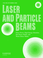
Thus, two ternary relations among (u, E, B),  $u=-\lpar {1}/{{\rm \mu} _{0}}\rpar \lpar {\lpar {\rm \partial} _{t}E-\nabla \times B\rpar }/{\lpar {\rm \varepsilon} _{0}\nabla \cdot E-ZeN_{i}\rpar }\rpar$ (derived from the Gauss law and the Ampere law) and Eq. (23), will lead to a binary relation between E and B. This binary relation combines with the Faraday law and $\nabla \cdot B=0$ will determine exact expressions of E and B in terms of (r, t). As shown in Figure 1, a self-consistent updating {r i} is thus obtained from RNEs under this exact expressions of E and B.

Fig. 1. Sketch of loyal and safe plasma simulation based on the N–M equations, where another ternary relation refers to “∂tp(u) + eE + eu × B = 0” and a ternary relation refers to  $u=-\lpar {1}/{{\rm \mu} _{0}}\rpar \lpar {\lpar {\rm \partial} _{t}E-\nabla \times B\rpar }/{\lpar {\rm \varepsilon} _{0}\nabla \cdot E-ZeN_{i}\rpar }\rpar$ which is derived from the Gauss law and the Ampere law.
The importance of such an RNE-derived ternary relation is self-evident. In particular, it can also be derived from complete mathematical description (Lin and Liu, Reference Lin and Liu2019b). In the complete description, the ME-side can yield a ternary relation  $u=-\lpar {1}/{{\rm \mu} _{0}}\rpar \lpar {\lpar {\rm \partial} _{t}E-\nabla \times B\rpar }/{\lpar {\rm \varepsilon} _{0}\nabla \cdot E-ZeN_{i}\rpar }\rpar$, and the VE and the inequality
 $$\eqalign{0&=\widehat{L}f \cr &=[ {\rm \partial} _t+{\rm \upsilon} \cdot \nabla -[ e[ E(r,t) +{\rm \upsilon} \times B(r,t) ] ] \cdot {\rm \partial} _{\rm p}]f \cr &=[ {\rm \partial} _t+u \cdot \nabla -e[ E+u \times B] \cdot {\rm \partial} _{\rm p}]f \cr &\quad +[{\rm \upsilon} -u]\cdot [\nabla-eB \times {\rm \partial} _{\rm p}]f;}$$
 $$0 \leq f\,({\rm \upsilon},r,t)\quad \forall {\rm \upsilon},r,t$$
can combine to yield another ternary relation among u,E,B (Fig. 2). Clearly, because of the linearity of the operator  $\widehat {L}$, if g 2 ≥ 0 can meet the VE, there will be $\widehat {L}g=0$. One can express g as power series of υ − u and $u\equiv {\int {\rm \upsilon} g^{2}\, {\rm d}^{3}{\rm \upsilon} }/{\int g^{2}\, {\rm d}^{3}{\rm \upsilon} }$:
 $$g\equiv g_{0}{\rm \delta} \lpar {\rm \upsilon} -u\rpar +\sum_{i\geq 1} g_{i}\Delta^{i}\semicolon\; $$
where Δ is defined as
 $$\Delta \equiv [ p\lpar {\rm \upsilon}\rpar -p\lpar u\rpar ] \times \exp\lpar -[ p\lpar {\rm \upsilon}\rpar -p\lpar u\rpar ] ^{2}\rpar \comma\; $$
and thus similar power series expression of g 2 reads
 $$g^{2}\equiv h_{0}{\rm \delta} \lpar {\rm \upsilon} -u\rpar +\sum_{i\geq 2} h_{i}\Delta^{i}$$
because of the unique property of the Dirac function (υ − u) × δ(υ − u) = 0. Thus, h 1 ≡ 0 is a universal property of solutions of the complete mathematical description (Lin and Liu, Reference Lin and Liu2019a). It will strictly, as shown elsewhere (Lin and Liu, Reference Lin and Liu2019a, Reference Lin and Liu2019b), lead to a ternary relation [Eq. (23)].
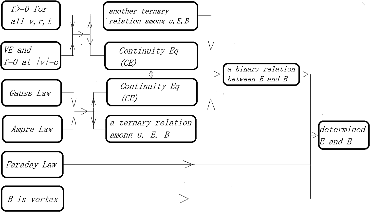
Fig. 2. Sketch of loyal and safe plasma simulation based on complete mathematical description, where another ternary relation refers to “∂tp(u) + eE + eu × B = 0” and a ternary relation refers to  $u=-\lpar {1}/{{\rm \mu} _{0}}\rpar \lpar {\lpar {\rm \partial} _{t}E-\nabla \times B\rpar }/{\lpar {\rm \varepsilon} _{0}\nabla \cdot E-ZeN_{i}\rpar }\rpar$ which is derived from the Gauss law and the Ampere law.
These relations for h i≥2 can be directly verified by substituting the series into the VE and comparing terms proportional to [p(υ) − p(u)]i order-by-order. Namely, the VE plays a role of a recurrence formula relating expansion coefficient functions in different orders, and those h i≥2 can be expressed by h 0 and u one-by-one. This well illustrates that the dependence of f on υ, or microscopic details of f, is governed by few macroscopic fields h 0 and u.
Comparison with interpolation-based particle simulation
Particle simulation is a series of stages in which the set {r i, d tr i; 1 ≤ i ≤ N p}t=(n+1)Δt is calculated from {r i, d tr i; 1 ≤ i ≤ N p}t=nΔt. The whole process is to allocate particles over different groups or cells. The set {r i, RV i; 1 ≤ i ≤ N p} is more appropriate to describe particles than the set {r i, d tr i; 1 ≤ i ≤ N p}, where the definition of the RV i(t) is as same as that of RV(r i(t), t), and hence, there exists a symmetry condition:
 $$\sum_{i}[ RV_{i}\lpar t\rpar \times {\rm \delta} \lpar r-r_{i}\lpar t\rpar \rpar ] = 0\quad \forall r\comma\; t.$$
 In the PIC simulation, even though electrons are classified according to their contributions to E,B, E,B are produced by  $\tilde {n}\comma\; \tilde {j}$ violating the CE and hence inexact. Now that sources of E,B satisfying the CE is mandatory for exactly solving the N–M system, the usage of the interpolation obviously disagrees with this purpose.
As far as electrons are concerned, the velocity of every electron, d tr j, consists of two parts: public part and private one. The public part, denoted as u(r j(t), t), has contribution to transverse-fields E tr, B, while the private part, denoted as RV(r j(t), t), has no contribution because the definition of two parts determine these private parts offsetting mutually. Thus, when N p particles are allocated into N c groups/cells (note that there is usually N p > N c), all particles within a group/cell have a same contribution, that is, the u-value of this cell, to n,j and hence E,B (because their RV-values offset mutually).
This fact enables the N–M system to display clearly a two-layer structure in which those RNEs/ODEs, beside yielding a ternary relationship among the public part and E,B, play a role of the definition of these private parts in terms of the public part and E,B. Thus, such a two-layer structure makes the N–M system to be solved without resorting to interpolation approximation and other unnecessary ones. This thoroughly ensures (E, B) being produced by (n, j) satisfying the CE and fundamentally warrant the reliability of particle simulation.
Summary
Keeping fluid equations valid under interpolation is a severe requirement on shape/interpolation functions adopted in the PIC simulation. Strict mathematics theory has denied existence of such shape/interpolation functions. Thus, it is no need to seek for the PIC solution of a N–M system because a better method is available.
Appendix
In both the N–M description and the V–M description, two MEs, the Gauss law and the Ampere law:
 $${\rm \varepsilon}_{0}\nabla \cdot E =-en +ZeN_i; $$
 $${\rm \partial} _tE ={\rm \mu}_{0}enu +\nabla \times B;$$
imply the CE
 $${1\over {\rm \varepsilon}_{0} {\rm \mu}_{0}}{\rm \partial}_{t}n+\nabla \cdot [ nu] =0\comma$$
and an expression of u, or a ternary relation among u,E,B:
 $$u=-{1\over {\rm \mu}_{0}}{{\rm \partial}_{t}E-\nabla \times B\over {\rm \varepsilon}_{0}\nabla \cdot E-ZeN_{i}},$$
where ɛ0 and μ0 are permittivity and permeability of vacuum, respectively, N i and n are ionic and electronic densities, respectively, Ze is charge per ion, u is fluid velocity, ions are viewed as fixed, and hence, ionic current is taken as 0. Here, Klimontovich–Dupree (K–D) definitions of n, j and u read (Krall and Trivelpiece, Reference Krall and Trivelpiece1977)
 $$n(r,t) \equiv \sum_i{\rm \delta} (r-r_i(t));$$
 $$j(r,t) \equiv \sum_id_{t}r_{i}{\rm \delta} (r-r_i(t));$$
 $$u(r,t) \equiv {\,j(r,t) \over n(r,t)},$$
where if n = 0, u = limn→0j/n is finite-valued because j → 0 exists when n → 0. Note that these K–D definitions can automatically warrant the CE and  $n\geq 0\, \ \forall r\comma\; t$ to be valid. Therefore, at particle positions where n,j,u are calculated according to the K–D definitions, the CE is valid. However, because n,j at mesh nodes are calculated, through the interpolation, from n,j at particle positions, whether the interpolation can warrant the CE to be valid at integer positions is very vital to the scientific validity of the whole PIC simulation.
In earlier PIC schemes, these shape/interpolation functions are often subjectively chosen to be a unary function of r − r i(t). For example, at page 411–412 in Dawson (Reference Dawson1983), Snf and Sjf are assumed/prescribed to be equal to a dimensionless unitary function S:
 $$\eqalign{\,j( r_{\rm m},t) &=\sum_i[S(r_i(t) -r_{\rm m}) \times j(r_i(t) ,t)],\cr n( r_{\rm m},t)& =\sum_i[S( r_i(t)-r_{\rm m}) \times n(r_i(t) ,t)],}$$
and detailed form of S is often subjectively chosen or prescribed to be area-weighted in 2D situation (see page 412 in Dawson, Reference Dawson1983), that is, S(r i(t) − r m) = (x i(t) − x m)/Δx × (y i(t) − y m)/Δy, where two constants Δx and Δy are the x-direction and y-direction steps of the 2D mesh. However, people have noticed that such a prescribed shape/interpolation function S can lead to the CE violated. For example, according to Eqs (A5)–(A7), the CE can be strictly satisfied at particle's position r i
 $${\rm \partial} _t n_{i}+\nabla _{r_i}\cdot j_{i}={\rm \partial} _t n(r_{i},t)+\nabla _{r_i}\cdot j(r_{i},t)=0.$$
Due to strict formulas
 $${\rm \partial} _t n_m =\sum_i[ S(r_i-r_{\rm m}) \times {\rm \partial} _t n_i] +\sum_i[ {\rm \partial} _tS(r_i-r_{\rm m}) \times n_i]$$
 $$\quad =\sum_i[ S(r_i-r_{\rm m}) \times {\rm \partial} _t n_i] +\sum_i[ d_tr_i \times S^{(1) }(r_i-r_{\rm m}) \times n_i]$$
 $$\nabla _{r_{\rm m}}\cdot j_{\rm m} =\sum_i[ \nabla _{r_{\rm m}}S(r_i-r_{\rm m})\times j_i]$$
 $$\quad =-\sum_i[S^{(1) }(r_i-r_{\rm m}) \times j_i]$$
there will be
 $$\eqalign{{\rm \partial} _t n_{\rm m}+\nabla _{r_{\rm m}}\cdot j_m &=\sum_i[ S(r_i-r_{\rm m}) \times {\rm \partial} _t n_i] +\sum_i[ d_tr_i\times S^{(1) }(r_i-r_{\rm m}) \times n_i] \cr &\quad -\sum_i[ S^{(1) }(r_i-r_{\rm m}) \times j_i]}$$
which implies that  $\partial _t n_{\rm m}+\nabla _{r_{\rm m}}\cdot j_{\rm m}=0$ will demand these S(r i − r m) to satisfy self-consistently a differential equation, rather than to be prescribed. It is straightforward to verify that above-mentioned subjectively chosen S = (x i(t) − x m)/Δx × (y i(t) − y m)/Δy cannot satisfy the above equation.
Moreover, strictly speaking, whether eight shape/interpolation functions can warrant four MEs satisfied should also be checked. For example, Faraday law should be valid not only at mesh nodes  $\nabla _{r_{\rm m}} \times E\lpar r_{\rm m}\comma\; t\rpar +{\rm \partial} _{t} B\lpar r_{\rm m}\comma\; t\rpar =0$ but also at particle positions $\nabla _{r_{i}\lpar t\rpar } \times E\lpar r_{i}\lpar t\rpar \comma\; t\rpar +{\rm \partial} _{t} B\lpar r_{i}\lpar t\rpar \comma\; t\rpar =0$. This needs to check whether shape/interpolation functions SEb and SBb can warrant MEs satisfied at particle's position. Likewise, $\nabla _{r_{i}}\cdot B_{i}=0=\nabla _{r_{\rm m}}\cdot B_{\rm m}$ demands $\nabla _{r_{\rm m}} \cdot SBf=0$ and $\nabla _{r_{i}} \cdot SBb=0$ satisfied.
It is easy to understand possible violations of these fluid equations. After being weighted summation through these shape/interpolation functions, these binary functions, such as n(r, t) and j(r, t), are “distorted”. Such distortions cannot always warrant previous space-time relations among these binary functions, which are defined by fluid equations, held after being interpolated. This fact excludes reasonability of subjectively choosing shape/interpolation functions.
After being aware of such a subjectively choice causing the violation of CE, people began to make some improvements (Esirkepov, Reference Esirkepov2001; Chen et al., Reference Chen, Chacon and Barnes2011; Markidis and Lapenta, Reference Markidis and Lapenta2011; Chen and Chacon, Reference Chen and Chacon2014, Reference Chen and Chacon2015), such as only a pair of shape/interpolation function, usually Snf and Snb, being subjectively chosen and other pairs being solved from the CE and hence functionals of Snf and Snb, for example, page 146–147 in Esirkepov (Reference Esirkepov2001). But because a pair of shape/interpolation function still can be subjectively chosen, all pairs of shape/interpolation functions is indeed still subjectively chosen or prescribed, rather than being self-consistently solved from the CE and MEs. Therefore, some authors turn their attention to other routes such as direct finite-difference calculation of the V–M system (Idomura et al., Reference Idomura, Ida, Kano, Aiba and Tokuda2008; Shiroto et al., Reference Shiroto, Ohnishi and Sentoku2019) because this route, despite too data-consuming, can warrant mass-conservation satisfied strictly.
Strictly speaking, what the PIC method do is merely to re-express the N p + 4 equations in terms of N p pairs of initial conditions (r i(t), d tr i(t))|t=0 and eight shape/interpolation functions, and hence, N p ODEs become difference equations of N d × N c × N p values of the Snf(r, r i(t)), where the value of N d is 4 for 2D situation and 12 for 3D situation (12 referring to a particle within the cell to be assigned to 12 mid-points in 12 laterals of the cubic cell). But such a set of difference equations is not solved, and instead, the solution of N d × N c × N p values of the Snf(r, r i(t)) is indeed assumed/prescribed. This fact, which refers to re-expressing what to be solved and prescribing its solutions, makes the PIC solution difficult to be trusted as a self-consistent solution of the N p + 4 equations.
Chen and Chacon noticed that these shape/interpolation functions should be self-consistently solved and made some progresses in 2D situation (Chen et al., Reference Chen, Chacon and Barnes2011; Chen and Chacon, Reference Chen and Chacon2014, Reference Chen and Chacon2015). They found that in 2D situation, when Sn is a B-spline function of order 2 and Sj is a B-spline function of order 1, the CE can be satisfied strictly (because of a special property of the B-spline function of order 2 pointed out in appendix in Chen et al. (Reference Chen, Chacon and Barnes2011)), if no particle exchange between cells occurs (or each particle's trajectory lies within a cell) (Chen and Chacon, Reference Chen and Chacon2015). These severe requirements on particles' positions and velocities, that is, no particle exchange between cells occurs (or each particle's trajectory lies within a cell), imply that these shape/interpolation functions found by Chen and Chacon are not universally applicable. Namely, a PIC simulation based on them needs non-self-consistently artificial interference for avoiding particle exchange between cells. This is fundamentally against the purpose of a first-principle calculation. Moreover, in more realistic 3D situation, this encouraging result, despite severe requirement on the absence of particle exchange between cells, does not hold because the B-spline function of order 3 does not have the above-mentioned special property held by the B-spline function of order 2).
Above contents have clearly answered why these shape/interpolation functions should be self-consistently solved, rather than prescribed. Now the problems are (1) how to solve and (2) whether a solution exists. If there is no clue for hinting how to solve them, one have to guess/assume trial analytic forms of eight shape/interpolation functions and check whether they can ensure four MEs, N p RNEs, and the CE satisfied. Clearly, such an exhaustive manner is less practical because it will drop into a cycle of repeatedly proposing an assumption and checking whether the assumption to be self-consistent (i.e., whether the assumed trial analytic forms can ensure the N p + 4 equations satisfied). Unfortunately, such a cycle is often non-controllable, that is, finding a self-consistent solution during finite rounds. In realistic 3D situation, people still frequently resort to subjectively cease such a non-controllable cycle.
If finding analytic forms of eight shape/interpolation functions is replaced by finding discrete values of 8 shape/interpolation functions, whether these discrete values can be solved depends on the number of equations they obey. In realistic 3D situation, if 12 × N c < N p, these is no solution of these discrete values. If 12 × N c > N p, these are multiple solutions of these discrete values.
If such self-consistent shape/interpolation functions, no matter in analytic form or in discrete expression, is unavailable, it will deny fundamentally necessity of seeking for the PIC solution of the N p + 4 equations.


