


1. Introduction
Following the seminal work by Bloom (Reference Bloom2009), there has been a vast amount of literature on how uncertainty negatively affects economic activity (Christiano et al. (Reference Christiano2014), Choi (Reference Choi2017), Bloom et al. (Reference Bloom2018)). For instance, when uncertainty rises, economic agents postpone their consumption or investment decisions and wait until the uncertainty is resolved to avoid downside risk. In previous studies, it has been widely analyzed whether the effects of monetary or fiscal policy depend on the level of economy-wide uncertainty, both theoretically and empirically. However, there has been little research into the interaction between uncertainty and macroeconomic policies. Most of the previous research assumes that uncertainty is exogenously given or at least is the most exogenous variable in the economy. This is a questionable assumption, as private agents consider policy action to be a major source of economic uncertainty and they expect policies to resolve uncertainty during economic downturns.
We answer the following two questions in this paper. First, how does uncertainty respond to real activity and to monetary policy? Second, how does the endogeneity of uncertainty alter the effectiveness of monetary policy? To this end, we provide a synthetic analysis of the joint dynamics of uncertainty and monetary policy using a modified shock-restricted structural vector-autoregression (VAR) model, as in Ludvigson et al. (Reference Ludvigson, Ma and Ng2021) (“LMN,” hereafter).
A preferable model for this study requires two features. First, the identification scheme needs to allow any possible degree of endogeneity in uncertainty. The identification scheme implemented in this paper is consistent with our goal, as it does not restrict the order of exogeneity nor the signs of the impulse responses. Instead, we impose restrictions on the behavior of the structural shocks, as in LMN. Second, we distinguish real and financial uncertainty and examine how they interact with policy action and real activity, following LMN and Jurado et al. (Reference Jurado, Ludvigson and Ng2015). In the literature, there have been various ways to look at uncertainty or at the uncertainty shock. Some researchers consider uncertainty to be a concept that originated from economic fundamentals, such as productivity (Christiano et al. (Reference Christiano2014), Gilchrist et al. (Reference Gilchrist, Sim and Zakrajšek2014), Bloom et al. (Reference Bloom2018), Park (Reference Park2019), ). On the other hand, other researchers argue that uncertainty affects the economy through financial markets and can be traced by indices describing financial market conditions, such as stock market volatility (Bekaert et al. (Reference Bekaert, Hoerova and Duca2013), Caggiano et al. (Reference Caggiano, Castelnuovo and Groshenny2014), Basu and Bundick (Reference Basu and Bundick2017), Choi et al. (Reference Choi2018)). This discrepancy may confuse discussions among researchers and affect the explanation as to the causes and consequences of uncertainty. For this reason, we separate real and financial uncertainty in a single framework to investigate the causes and consequences of each type of uncertainty.
Our main findings are as follows. While in LMN financial uncertainty is an exogenous impulse of business cycle fluctuations, we show that in our model, both real and financial uncertainties are endogenous responses of business cycle fluctuations. Second, unlike Bekaert et al. (Reference Bekaert, Hoerova and Duca2013), the contractionary monetary policy shock reduces financial uncertainty while it exacerbates real uncertainty at the same time in our identifying restrictions. We show that allowing contemporaneous interactions between the aggregate economy and uncertainty plays an important role in determining the impact of monetary policy on financial uncertainty through the counterfactual study. In particular, once we shut down the contemporaneous responses of uncertainties, as in Carriero et al. (Reference Carriero, Clark and Marcellino2021), it turns out that the contractionary monetary policy shock increases financial uncertainty, which is more in line with Bekaert et al. (Reference Bekaert, Hoerova and Duca2013). Finally, it is shown that the endogeneity of uncertainty plays an amplifying role in the efficacy of monetary policy. To be precise, the responsiveness of real activity with respect to monetary policy shocks in the benchmark model is higher than that in the counterfactual model that shuts down the endogeneity channel.
Related literature. This paper is closely related to the uncertainty literature pioneered by Bloom (Reference Bloom2009). The main difference between this paper and previous studies is that we investigate a model of endogenous uncertainty, while previous ones considered uncertainty shocks that were independent of economic activity. Based on the exogeneity assumption, we analyze the roles of uncertainty shocks as a business cycle driver (Bloom (Reference Bloom2009), Christiano et al. (Reference Christiano2014), Bloom et al. (Reference Bloom2018)) and as a source of monetary (Castelnuovo and Pellegrino (Reference Castelnuovo and Pellegrino2018), Pellegrino (Reference Pellegrino2018a, b)) and fiscal policy (Berg (Reference Berg2019)) asymmetry.Footnote 1 To summarize these previous studies, uncertainty shocks depress economic activity and dampen the effectiveness of monetary policy all while stimulating the effectiveness of fiscal policy. This paper differs from that, as we track the importance of the endogenous movements of uncertainty on macroeconomic developments.
This paper is not the first paper to explore endogenous uncertainty. Bachmann and Moscarini (Reference Bachmann and Moscarini2011) noticed that negative first-moment shocks can induce volatile and dispersed outcomes, that is, uncertainty. Fajgelbaum et al. (Reference Fajgelbaum, Schaal and Taschereau-Dumouchel2017) provided a novel framework for endogenous uncertainty through social learning and showed that vicious cycles can rise as decreased investments can reduce information flows, which are necessary to remove uncertainty. Also, Guimaraes et al. (Reference Guimaraes, Machado and Ribeiro2016) showed in a static model how fiscal policy affects the aggregate economy through the confidence channel. In their model, increased government spending signals more private investment; hence, it prevents a coordination failure that would arise due to imperfect information about the fundamentals. Bekaert et al. (Reference Bekaert, Hoerova and Duca2013) study a similar topic to ours, as they analyze how monetary policy affects risk appetite and uncertainty. They find that a lax monetary policy decreases uncertainty. Ours differs from this, as we distinguish real and financial uncertainty. Carriero et al. (Reference Carriero, Clark and Marcellino2021) are also closely related to this paper. They also examine to what extend the endogenous responses of macroeconomic (real) or financial uncertainty matter for macroeconomic dynamics. They report that macroeconomic uncertainty can be considered to be exogenous, but that financial uncertainty is not. However, they do not consider the impact of monetary policy on uncertainty, which is the primary concern in this research.
The rest of the paper is organized as follows. Section 2 introduces the empirical strategy that allows us to investigate the relationship between uncertainty and monetary policy. Section 3 explains the results obtained from our empirical analysis in detail. Section 4 concludes the paper.
2. Empirical framework
In this section, we explain the empirical strategy employed in this paper to analyze the interaction between uncertainty and monetary policy and its influence on real activity. In particular, our baseline empirical model is mainly based on that used in LMN. LMN use a three-variable VAR model that consists of variables that represent real uncertainty, real activity, and financial uncertainty to show whether uncertainties, which rise in recessions, are sources of the business cycle, or are endogenous responses to it. In this paper, we extend that model to analyze the effects of monetary policy. We use this state-of-the-art model, as it is of utmost importance to carefully identify different types of uncertainty in a unified empirical framework to study the interactions among monetary policy, real activity, and uncertainty.
To be precise, we build a five-variable VAR model that includes real and financial uncertainty, real output, the price index, and a monetary policy indicator. The VAR model used in this paper is basically identified by the shock restriction method applied in LMN that was originally proposed by Ludvigson et al. (Reference Ludvigson, Ma and Ng2017).
2.1 Data
In the baseline model, we use monthly data from October 1980 to December 2018. First, the estimated monthly real GDPFootnote 2 provided by two sources is used to measure the real activity in the monthly model. We use monthly estimates of GDP provided by Mark Watson, which cover January 1959 to June 2010, and from Macroeconomic Advisers by IHS Markit, which cover January 1992 to August 2019.Footnote 3 We first check that the movements from the two sources are almost the same for the overlapped periods and that the correlation coefficient is close to unity. Then, we merge the datasets with some adjustments to eliminate any differences in the overall levels that may be caused by differences in the base years. For the price index, we use the monthly Core Personal Consumption Expenditure (PCE) index which excludes price shifts in the food and energy sectors.Footnote 4
As measures of real and financial uncertainty, the measures proposed in Jurado et al. (Reference Jurado, Ludvigson and Ng2015) and LMN are used.Footnote
5
The measured uncertainties are closely related to forecasting errors. To better understand, let us define $y_{jt}^C$
, a variable related to the real (
$y_{jt}^C$
, a variable related to the real ( $R$
) and financial (
$R$
) and financial ( $F$
) economy, specified by the category indicator
$F$
) economy, specified by the category indicator $C\in \{R,F\}$
. Then, the
$C\in \{R,F\}$
. Then, the $h$
-period ahead purely unforecastable component of
$h$
-period ahead purely unforecastable component of $y_{jt}^C$
, conditional on all information available at time
$y_{jt}^C$
, conditional on all information available at time $t$
,
$t$
, $\mathcal{U}_{jt}^C(h)$
is formulated in this way:
$\mathcal{U}_{jt}^C(h)$
is formulated in this way:
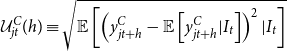 \begin{equation} \mathcal{U}_{jt}^C(h)\equiv \sqrt{\mathbb{E}\left [\left (y_{jt+h}^C-\mathbb{E}\left [y_{jt+h}^C|I_t\right ]\right )^2|I_t\right ]} \end{equation}
where $I_t$
represents the information set at time
$I_t$
represents the information set at time $t$
. Then, the measured uncertainty
$t$
. Then, the measured uncertainty $U_{Ct}$
is the weighted sample average of
$U_{Ct}$
is the weighted sample average of $\mathcal{U}_{jt}^C(h)$
. We use one-month ahead forecast uncertainty (
$\mathcal{U}_{jt}^C(h)$
. We use one-month ahead forecast uncertainty ( $h=1$
) as the benchmark variable following LMN, but the main results are not affected by changing the forecast uncertainty horizon to
$h=1$
) as the benchmark variable following LMN, but the main results are not affected by changing the forecast uncertainty horizon to $h=6$
or
$h=6$
or $h=12$
.
$h=12$
.
As a variable that summarizes the monetary policy stance, we use the one-year government bond yield in the baseline analysis, following Gertler and Karadi (Reference Gertler and Karadi2015). This variable is employed as the policy indicator, as it is highly correlated with the monetary policy instrument, the federal funds rate (FFR), but is not subject to the zero lower bound during the sample period.Footnote 6 Based on the choice of monetary policy variable, the monetary policy shock that measures the unexpected changes in the stance of the monetary authority is identified by introducing an auxiliary instrument variable. Specifically, the monetary policy news shock identified in Nakamura and Steinsson (Reference Nakamura and Steinsson2018) is employed as an instrument to help identify the monetary policy shock.
As will be explained in the subsequent subsections, we incorporate two external instruments— $S_{1t}$
, the return on the S
$S_{1t}$
, the return on the S $\&$
P 500 index, and,
$\&$
P 500 index, and, $S_{2t}$
, the log difference of the real gold price—as in LMN, to identify the two types of uncertainty shocks.Footnote
7
$S_{2t}$
, the log difference of the real gold price—as in LMN, to identify the two types of uncertainty shocks.Footnote
7
2.2 The Structural VAR (SVAR) and identification
2.2.1 The model
Let $X_{t}$
be the five-by-one endogenous variable. The reduced form VAR model can be expressed as
$X_{t}$
be the five-by-one endogenous variable. The reduced form VAR model can be expressed as
 \begin{equation} X_{t}=k_{t}+A_{1}X_{t-1}+A_{2}X_{t-2}+\cdots +A_{p}X_{t-p}+\eta _{t} \end{equation}
where $\eta _{t}\sim (0,\Omega )$
is the reduced form residual and
$\eta _{t}\sim (0,\Omega )$
is the reduced form residual and $k_{t}$
is the vector of exogenous variables, including the constant, linear, and quadratic time trends.Footnote
8
The lag order is chosen to be two based on the Schwarz information criterion.
$k_{t}$
is the vector of exogenous variables, including the constant, linear, and quadratic time trends.Footnote
8
The lag order is chosen to be two based on the Schwarz information criterion.
The structural shocks $e_{t}$
are related to the reduced form residuals as
$e_{t}$
are related to the reduced form residuals as
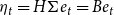 \begin{equation} \eta _{t}=H\Sigma e_{t}=B e_{t} \end{equation}
where $e_{t}\sim (0,\mathbf{I_{k}})$
,
$e_{t}\sim (0,\mathbf{I_{k}})$
, $H\Sigma$
is a variance-covariance matrix of
$H\Sigma$
is a variance-covariance matrix of $\eta$
and
$\eta$
and $\Sigma$
is the diagonal variance matrix.
$\Sigma$
is the diagonal variance matrix.
The endogenous variable is set as $X_{t}=(U_{Rt},GDP_{t},PCE_{t},U_{Ft},MP_{t})'$
.
$X_{t}=(U_{Rt},GDP_{t},PCE_{t},U_{Ft},MP_{t})'$
. $U_{Rt}$
,
$U_{Rt}$
, $GDP_{t}$
,
$GDP_{t}$
, $PCE_{t}$ $U_{Ft}$
and
$U_{Ft}$
and $MP_{t}$
denote real uncertainty (RU), real GDP (RGDP), core personal consumption expenditure (PCE), financial uncertainty (FU), and the monetary policy (MP) indicator. The corresponding reduced form residuals
$MP_{t}$
denote real uncertainty (RU), real GDP (RGDP), core personal consumption expenditure (PCE), financial uncertainty (FU), and the monetary policy (MP) indicator. The corresponding reduced form residuals $\eta _{t}=(\eta _{Rt},\eta _{GDPt},\eta _{PCEt},\eta _{Ft},\eta _{MPt})'$
can be related to the structural shocks
$\eta _{t}=(\eta _{Rt},\eta _{GDPt},\eta _{PCEt},\eta _{Ft},\eta _{MPt})'$
can be related to the structural shocks $e_{t}=(e_{Rt},e_{GDPt},e_{PCEt},e_{Ft},e_{MPt})'$
as below:
$e_{t}=(e_{Rt},e_{GDPt},e_{PCEt},e_{Ft},e_{MPt})'$
as below:
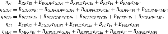 \begin{equation} \begin{split} \eta _{Rt}&=B_{RR}e_{Rt}+B_{RGDP}e_{GDPt}+B_{RPCE}e_{PCEt}+B_{RF}e_{Ft}+B_{RMP}e_{MPt}\\ \eta _{GDPt}&=B_{GDPR}e_{Rt}+B_{GDPGDP}e_{GDPt}+B_{GDPPCE}e_{PCEt}+B_{GDPF}e_{Ft}+B_{GDPMP}e_{MPt}\\ \eta _{PCEt}&=B_{PCER}e_{Rt}+B_{PCEGDP}e_{GDPt}+B_{PCEPCE}e_{PCEt}+B_{PCEF}e_{Ft}+B_{PCEMP}e_{MPt}\\ \eta _{Ft}&=B_{FR}e_{Rt}+B_{FGDP}e_{GDPt}+B_{FPCE}e_{PCEt}+B_{FF}e_{Ft}+B_{FMP}e_{MPt}\\ \eta _{MPt}&=B_{MPR}e_{Rt}+B_{MPGDP}e_{GDPt}+B_{MPPCE}e_{PCEt}+B_{MPF}e_{Ft}+B_{MPMP}e_{MPt}\\ \end{split} \end{equation}
where $B_{ij}$
is the element that belongs to
$B_{ij}$
is the element that belongs to $B$
.Footnote
9
As is evident from the above relationships, identifying structural shocks corresponds to finding a solution for the matrix
$B$
.Footnote
9
As is evident from the above relationships, identifying structural shocks corresponds to finding a solution for the matrix $B$
. The standard covariance restrictions, which come from the covariance structure of
$B$
. The standard covariance restrictions, which come from the covariance structure of $\eta _{t}$
, provide
$\eta _{t}$
, provide $15(\!=\!5\times 6/2)$
equations in
$15(\!=\!5\times 6/2)$
equations in $B$
and there are
$B$
and there are $25(\!=\!5\times 5)$
unknowns in
$25(\!=\!5\times 5)$
unknowns in $B$
. Hence, we need ten additional restrictions to exactly identify all the structural shocks. Therefore, it is not possible to exactly identify the structural shocks without further identifying assumptions. In this paper, we do not pursue a point identification but a set identification as in LMN to consider all possible solutions under our restriction.
$B$
. Hence, we need ten additional restrictions to exactly identify all the structural shocks. Therefore, it is not possible to exactly identify the structural shocks without further identifying assumptions. In this paper, we do not pursue a point identification but a set identification as in LMN to consider all possible solutions under our restriction.
2.2.2 Shock-based restrictions
In what follows, we introduce additional identifying assumptions that are required in order to obtain the structural relationships among endogenous variables. The key idea here is that the resulting structural shocks $e_{t}$
depend on the matrix
$e_{t}$
depend on the matrix $B$
. Hence, by looking at the characteristics of candidate structural shocks, we can gather additional information that can be used to judge whether the candidate matrix
$B$
. Hence, by looking at the characteristics of candidate structural shocks, we can gather additional information that can be used to judge whether the candidate matrix $B$
should be accepted or discarded.
$B$
should be accepted or discarded.
External variable constraints. First, we augment the external instrumental variables to provide more restrictions, following LMN. Specifically, the correlations between the external variables and the uncertainty shocks are used to provide additional inequality constraints. The aggregate stock market return $S_{1t}$
and the log difference in the real price of gold
$S_{1t}$
and the log difference in the real price of gold $S_{2t}$
are required to satisfy the following restrictions:
$S_{2t}$
are required to satisfy the following restrictions:
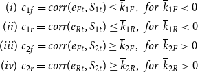 \begin{equation} \begin{split} (i) & \:\: c_{1f}=corr(e_{Ft},S_{1t})\leq \overline{k}_{1F}, \:\: for \:\: \overline{k}_{1F}\lt 0\\ (ii) & \:\: c_{1r}=corr(e_{Rt},S_{1t})\leq \overline{k}_{1R}, \:\: for \:\: \overline{k}_{1R}\lt 0\\ (iii) & \:\: c_{2f}=corr(e_{Ft},S_{2t})\geq \overline{k}_{2F}, \:\: for \:\: \overline{k}_{2F}\gt 0\\ (iv) & \:\: c_{2r}=corr(e_{Rt},S_{2t})\geq \overline{k}_{2R}, \:\: for \:\: \overline{k}_{2R}\gt 0 \end{split} \end{equation}
The first constraint states that the structural financial uncertainty shock should be negatively correlated with aggregate stock market returns. Similarly, the second one dictates that the structural real uncertainty shock is required to be negatively correlated with the stock market returns. Symmetrically, the third and last one implies that the structural shocks of financial and real uncertainty need to be positively correlated with the real price of gold. These restrictions are based on the broad consensus that stock market returns and the price of gold are closely related to financial and real uncertainty, respectively.
In addition, we introduce an external instrument to help identify the monetary policy shock. To be precise, it is required to have the minimal correlation $\overline{k}_{MP}$
with the monetary policy news shock
$\overline{k}_{MP}$
with the monetary policy news shock $S_{3t}$
identified in Nakamura and Steinsson (Reference Nakamura and Steinsson2018), as shown below.
$S_{3t}$
identified in Nakamura and Steinsson (Reference Nakamura and Steinsson2018), as shown below.
 \begin{equation} \begin{split} (v) & \:\: c_{3}=corr(e_{MPt},S_{3t})\geq \overline{k}_{MP} \end{split} \end{equation}
We also add a restriction so that the correlation between the structural real output shock $e_{GDPt}$
and the measured total factor productivity (TFP)
$e_{GDPt}$
and the measured total factor productivity (TFP) $S_{4t}$
should be greater than a certain threshold. By doing this, we allow the possibility of a slight lag or lead relationship between the two variables. To be precise, we impose the behaviors of structural aggregate supply shocks as follows.
$S_{4t}$
should be greater than a certain threshold. By doing this, we allow the possibility of a slight lag or lead relationship between the two variables. To be precise, we impose the behaviors of structural aggregate supply shocks as follows.
 \begin{equation} \begin{split} (vi) & \:\: c_{4}=\max\!\left \{corr(e_{GDPt},S_{4t}),corr(e_{GDP,t-1},S_{4t}),corr(e_{GDPt},S_{4,t-1})\right \}\geq \overline{k}_{real} \end{split} \end{equation}
Event constraints. Event constraints restrict the behavior of the structural shocks based on a reading of the times throughout history. The idea is that the produced structural shocks should be consistent with our understanding of historical events, at least during times of special interest. Again, we rely on LMN to construct event constraints below.
-
1. $e_{Ft_{1}}\gt \overline{k}_{1}$
where
$t_{1}$
is the period 1987 : 10 of the stock market crash
$e_{Ft_{1}}\gt \overline{k}_{1}$
where
$t_{1}$
is the period 1987 : 10 of the stock market crash -
2.
$e_{Ft_{2}}\gt \overline{k}_{2}$
where
$t_{2}=$
2008 : 09 -
3.
$\sum _{j=t_{3}}e_{GDPt}\lt \overline{k}_y$
,
$t_{3} \in [2007\;:\;12,2009\;:\;06]$
,
$\overline{k}_y\lt 0$
-
4.
$e_{Rt_{4,1}}\gt \bar{k}_{4r1}$
at
$t_{4,1}=2011\;:\;07$
or
$e_{Rt_{4,2}}\gt \bar{k}_{4r2}$
at
$t_{4,2}=2011\;:\;08$
-
5.
$e_{Ft_{4,1}}\gt \bar{k}_{4f1}$
at
$t_{4,1}=2011\;:\;07$
or
$e_{Ft_{4,2}}\gt \bar{k}_{4f2}$
at
$t_{4,2}=2011\;:\;08$


The above set of restrictions demands specific signs and sizes for the identified shocks. Firstly, the identified financial uncertainty shocks in October 1987 should be large, exceeding the $\overline{k}_{1}$
standard deviations, and positive. Second, the identified financial uncertainty in September 2008, which is the month of the Lehman collapse, should be large and exceed the
$\overline{k}_{1}$
standard deviations, and positive. Second, the identified financial uncertainty in September 2008, which is the month of the Lehman collapse, should be large and exceed the $\overline{k}_{2}$
standard deviations above the mean.Footnote
10
The third restriction requires that the cumulative GDP shocks during the [2007:12,2009:06] period should be less than a certain negative number.Footnote
11
The fourth and fifth conditions state that both the financial and real uncertainty shock should be positive during the 2011 debt ceiling crisis. To be precise, they should be positive either in July 2011 or in August 2011.
$\overline{k}_{2}$
standard deviations above the mean.Footnote
10
The third restriction requires that the cumulative GDP shocks during the [2007:12,2009:06] period should be less than a certain negative number.Footnote
11
The fourth and fifth conditions state that both the financial and real uncertainty shock should be positive during the 2011 debt ceiling crisis. To be precise, they should be positive either in July 2011 or in August 2011.
Finally, we find the max-C solution that has the maximal absolute correlation between the identified structural shocks and the external instrument variables, as shown in equation (8) where $c(B)=[c_{1f} \:\: c_{1r} \:\: c_{2f} \:\: c_{2r} \:\: c_{3} \:\: c_{4}]'$
. That is, the max-C solution is the solution with the highest collective correlation
$c(B)=[c_{1f} \:\: c_{1r} \:\: c_{2f} \:\: c_{2r} \:\: c_{3} \:\: c_{4}]'$
. That is, the max-C solution is the solution with the highest collective correlation $\sqrt{c(B)'c(B)}$
. Although no single solution is more likely than another, we provide this exact solution as a reference solution to the model. In the subsequent sections, we use the max-C solution as the reference result and pay more attention to this specific solution.
$\sqrt{c(B)'c(B)}$
. Although no single solution is more likely than another, we provide this exact solution as a reference solution to the model. In the subsequent sections, we use the max-C solution as the reference result and pay more attention to this specific solution.
 \begin{equation} \hat{B}_{\text{max-C}}=\mathop{\textrm{argmax}}_{B}\sqrt{c(B)'c(B)} \end{equation}
2.2.3 Implementation
The candidate solutions $\hat{B}$
are obtained by following LMN. Specifically, we initialize the solution to be the lower Cholesky factorization of
$\hat{B}$
are obtained by following LMN. Specifically, we initialize the solution to be the lower Cholesky factorization of $\Omega$
and then rotate it by 15,000,000 random orthogonal matrices
$\Omega$
and then rotate it by 15,000,000 random orthogonal matrices $Q$
. We keep the resulting solutions only when all restrictions given above are satisfied.
$Q$
. We keep the resulting solutions only when all restrictions given above are satisfied.
It is crucial to reasonably choose the numerical bounds of correlation and event constraints, as they determine the acceptance rate of candidate solutions. To fix the thresholds in a reasonable way, we choose $\bar{k}$
s from the sample distribution drawn from the simulations. That is, we first draw random orthogonal matrices
$\bar{k}$
s from the sample distribution drawn from the simulations. That is, we first draw random orthogonal matrices $Q(5 \times 5)$
and simulate arbitrary structural shocks without any restriction. From the simulation, we obtain the set of correlations between structural shocks and external variables, and the size of structural shocks for certain events.
$Q(5 \times 5)$
and simulate arbitrary structural shocks without any restriction. From the simulation, we obtain the set of correlations between structural shocks and external variables, and the size of structural shocks for certain events.
We report sets of all possible structural shocks drawn from 15,000,000 random draws in Section B. Figure 8a shows the distribution of correlations between structural shocks and external variables, and Figure 8b depicts the distribution for the size of structural shocks for each event. Given the empirical distributions of correlation coefficients and those of the size of shocks during certain historical events, we choose our $\bar{k}$
s as in Table 1.
$\bar{k}$
s as in Table 1.
Implementation of shock restrictions. A visual representation of all simulated random shocks in Section B
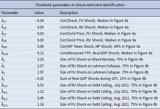
As shown in Table 1, most correlation constraints are set to medians of each sample distribution in Figure 8a to be conservative regarding the relationships between structural shocks and instrument variables, except $\bar{k}_{MP}$
—the constraint for the correlation between Nakamura and Steinsson (Reference Nakamura and Steinsson2018) news shocks and monetary structural shocks. We impose relatively stronger criteria for
$\bar{k}_{MP}$
—the constraint for the correlation between Nakamura and Steinsson (Reference Nakamura and Steinsson2018) news shocks and monetary structural shocks. We impose relatively stronger criteria for $\bar{k}_{MP}$
since the instrument used is conceptually identical to the shock that we would like to identify. Moreover, it also helps to resolve the “price puzzle” that arises in the standard monetary VAR.
$\bar{k}_{MP}$
since the instrument used is conceptually identical to the shock that we would like to identify. Moreover, it also helps to resolve the “price puzzle” that arises in the standard monetary VAR.
For the event constraints, most restrictions on the size of the structural shock for each event are set to the 75th percentile of each sample distribution in Figure 8b. The exception is $\bar{k}_y$
, the threshold for the sum of the real GDP shock during the Global Financial Crisis (GFC). We choose the stricter restriction for this threshold to ensure that the real GDP shocks are sufficiently small during that period. As shown in Figure 7 in the Online Appendix, the empirically measured total factor productivity (TFP) during the GFC shows a large drop for the TFP. Hence, we impose a restriction so that the sum of the structural real GDP shocks during the GFC should be sufficiently large in terms of size.Footnote
12
$\bar{k}_y$
, the threshold for the sum of the real GDP shock during the Global Financial Crisis (GFC). We choose the stricter restriction for this threshold to ensure that the real GDP shocks are sufficiently small during that period. As shown in Figure 7 in the Online Appendix, the empirically measured total factor productivity (TFP) during the GFC shows a large drop for the TFP. Hence, we impose a restriction so that the sum of the structural real GDP shocks during the GFC should be sufficiently large in terms of size.Footnote
12
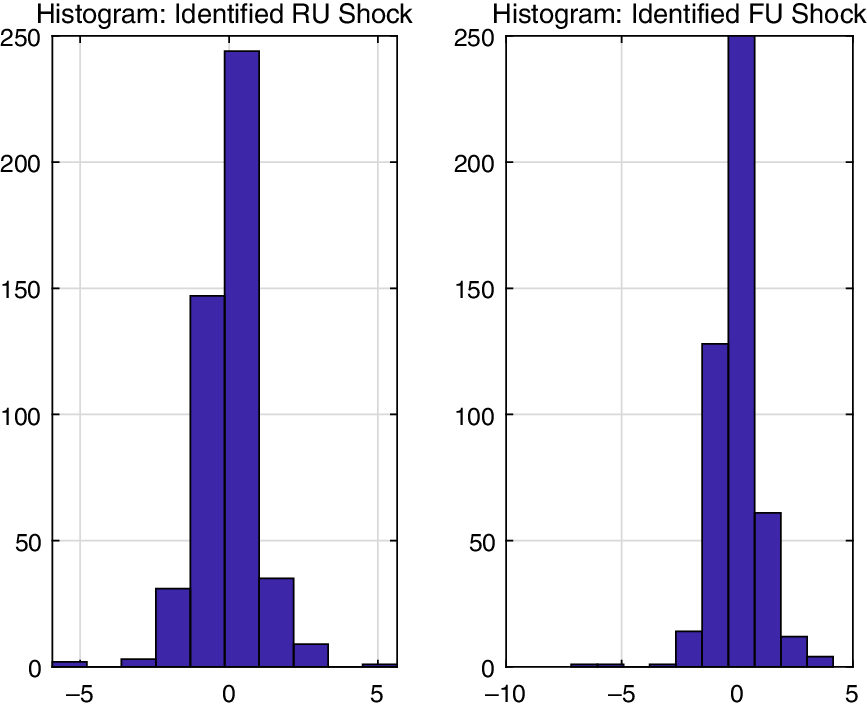
Finally, we depict the histograms of identified shocks produced in the max-C solution, following LMN. In the main text, we only report the identified real and financial uncertainty shocks as this research focuses on the behavior and consequences of the uncertainties. In addition, we also show that our identified structural output shock is consistent with the TFP to emphasize the validity of the identification scheme in Section A.
Figure 1 shows the set of the identified real and financial uncertainty shocks using histogram plots. It shows that the identified shocks are non-Gaussian. In particular, the max-C solutions of financial uncertainty shocks are skewed and have fat tails. Since the structural shocks of both the real and financial uncertainty are negatively skewed and since they have large values for the kurtosis, it supports our empirical strategy that does not require any Gaussian assumption.
Histogram of identified shocks: The left panel shows the density of the identified real uncertainty shock, and the right panel presents that of the financial uncertainty shock. The skewness and kurtosis of the real uncertainty shock are *0.5301 and 10.1395, respectively. Those of the financial uncertainty shock are *0.6198 and 11.0202, respectively.
3. Results
In this section, we present the results derived from the SVAR model constructed in the previous section. To do this, the full impulse response functions are shown to gauge the effects of each structural shock. In particular, we are interested in the responses of real and financial uncertainty to the monetary policy shock, as there is little previous research on the roles of monetary policy in shaping different types of economic uncertainty. In addition, we revisit the issue related to the endogeneity of economic uncertainty and analyze whether uncertainty is a driver of economic fluctuations or whether it is a consequence of them.
3.1 Interactions between uncertainty and monetary policy
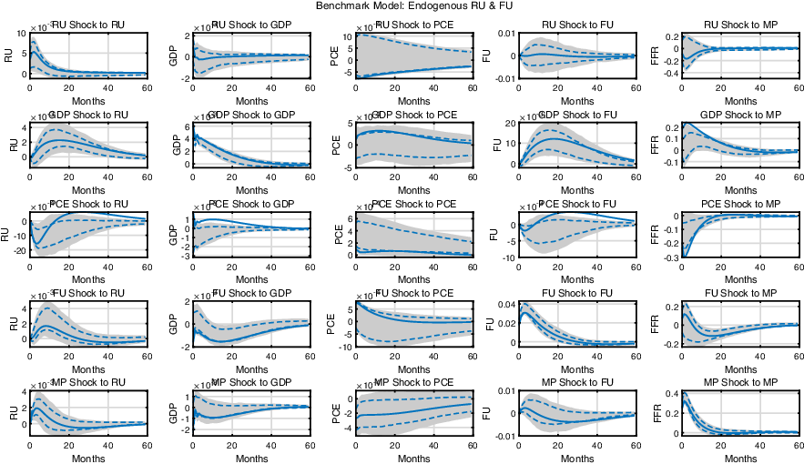
Figure 2 depicts the impulse responses of the SVAR model. When constructing the impulse responses, we use the bootstrap method, as suggested in LMN, to construct the confidence intervals of the impulse responses.Footnote 13 We focus here more on the responses to structural shocks regarding real uncertainty, real GDP, financial uncertainty, and monetary policy.
Impulse response functions of the monetary SVAR model: The shaded area and the dashed lines represent the 90% and 68% confident intervals, and the solid lines represent the max-C impulse responses.
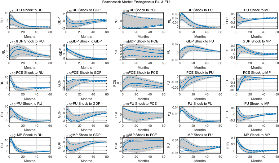
The first row shows the responses of the endogenous variables to the real uncertainty (RU) shock. It shows that a positive structural RU shock decreases real GDP, but has an insignificant effect on the price level. Note that a positive RU shock in LMN, on the contrary, increased the real GDP. They argue that their results are consistent with the growth option theory.Footnote 14 This would imply, on the other hand, that our results are more in line with the real option theory—heightened uncertainty leads to a recession as economic agents postpone decisions (e.g. Bernanke (Reference Bernanke1983)). This is more consistent with the findings in the other studies, such as Carriero et al. (Reference Carriero, Clark and Marcellino2021), inter alia. Finally, a hike in real uncertainty leads to an expansionary monetary policy. This policy action may be caused by the policy action to offset the economic contraction following the real uncertainty shock.
The second row represents responses to the positive structural real GDP shock. The real GDP shock increases both RU and financial uncertainty (FU). Thus, both RU and FU endogenously respond to business cycle fluctuations. These results differ from those in LMN, as they find that an increase in real activity leads to lower real uncertainty and higher financial uncertainty. We believe that this distinction arises due to the omitted influence of monetary policy in LMN. As a monetary policy measure is absent in LMN, the identified real activity shock in their study might include some influence of monetary policy shifts. A common finding that financial uncertainty increases in a GDP shock might be understood as climbing up a boom phase of the financial cycle (Brunnermeier and Sannikov (Reference Brunnermeier and Sannikov2014), Borio (Reference Borio2014), Filardo and Rungcharoenkitkul (Reference Filardo and Rungcharoenkitkul2016)). As the economy expands, market participants take more risk and credit accumulates. These behaviors lead to financial imbalances and worsen the financial cycle. Finally, monetary policy gets tighter for about 30 months following a positive GDP shock. This reaction can be understood as an ordinary monetary policy reaction to prevent the economy from becoming overheated. Combining the results obtained in the first and second row, it can be inferred that shifts in real uncertainty are a consequence of the business cycle, but that they can also be considered as an exogenous cause of fluctuations. This result contrasts with that of LMN, which finds that real uncertainty is largely a consequence of business cycle fluctuations, and to that in Carriero et al. (Reference Carriero, Clark and Marcellino2021), in which they document that real uncertainty can be considered as exogenous to any fluctuations. Put differently, our results suggest that real uncertainty can be considered as both a driver and a consequence of business cycles.
The fourth row shows the impulse responses to a positive financial uncertainty shock. Real uncertainty shows a positive hump-shaped response to the financial uncertainty shock. The above results clearly show that real and financial uncertainty co-move and are intertwined. Next, a rise in financial uncertainty leads to an immediate decline in GDP. This result is in line with many previous studies, which document that uncertainty drags down real activity (Bloom (Reference Bloom2009), Caggiano et al. (Reference Caggiano, Castelnuovo and Groshenny2014), Christiano et al. (Reference Christiano2014), Bloom et al. (Reference Bloom2018)). As the shock depresses real activity, a monetary accommodation follows to stimulate the economy in times of recession. The monetary policy response to the financial uncertainty shock is in line with that of Bekaert et al. (Reference Bekaert, Hoerova and Duca2013) and Carriero et al. (Reference Carriero, Clark and Marcellino2021). Central banks maintain a lax monetary policy following a rise in financial uncertainty. The results derived so far lend support to the view that heightened financial uncertainty can be both a cause and a consequences of business cycle fluctuations.
To summarize, our results are somewhat different from those in LMN or Carriero et al. (Reference Carriero, Clark and Marcellino2021). LMN reports that real uncertainty is an endogenous response rather than an exogenous impulse to business cycle fluctuations, while the opposite is true for financial uncertainty. Carriero et al. (Reference Carriero, Clark and Marcellino2021) document that real uncertainty can be considered as exogenous, but that financial uncertainty cannot. On the contrary, our results point out that both RU and FU can be considered to be both drivers and consequences of business cycle fluctuations at the same time.
The final row depicts the propagation of a positive monetary policy shock. Monetary tightening results in a slowdown in real activity while the price level decreases, as predicted by a vast amount of monetary literature (e.g. Christiano et al. (Reference Christiano, Eichenbaum and Evans2005), inter alia). This result can be considered as additional evidence of the plausibility of our identification scheme. Real and financial uncertainty show distinct reactions to the monetary policy shock. Real uncertainty increases substantially while financial uncertainty persistently decreases. This contradicts the outcomes explored in Bekaert et al. (Reference Bekaert, Hoerova and Duca2013), as they predicted the opposite effects of monetary policy on financial uncertainty: a lax monetary policy action decreases financial uncertainty, while this effect is not strong. Since their results have been accepted widely in the literature, we provide additional analysis of these results in the subsequent subsection. Our findings that financial uncertainty decreases in the policy rate may be attributed to unwinding financial stress or unbalances: by increasing the policy rate, the monetary authority may prevent financial markets from bearing more risk and prevent the piling-up of financial unbalances or bubbles (Rajan (Reference Rajan2005), Adrian and Liang (Reference Adrian and Liang2018), Ajello et al. (Reference Ajello, Laubach, López-Salido and Nakata2019)). In addition, they also find that the degree of risk aversion increases with the monetary policy stance.Footnote 15 This result may be related to our result that real uncertainty moves in the same direction as monetary policy, as a higher risk aversion leads to stronger wait-and-see behavior, which prevails under higher real uncertainty.
The above results bear clear new policy implications. In particular, they are closely related to the view that a monetary authority needs to monitor the financial cycle to prevent any severe recession caused by busts in financial markets (Adrian & Shin, Reference Adrian and Shin2008)). The response of financial uncertainty hints that a tightening in the monetary policy stance may reduce risk-taking, relieve financial uncertainty, and prevent the creation of bubbles. However, risk management through conventional monetary policy should be carried out cautiously, as it can also increase uncertainty related to real activities and incur immediate costs related to shrinking real activity. In sum, monetary policy seems to have a significant counter-cyclical effect in the short- to medium-term, while it also affects the buildup of uncertainties.
3.2 Role of endogenous responses of uncertainties
In this subsection, we analyze the importance of the endogenous responses of uncertainties to the monetary policy shock while conducting policy analyses. Specifically, we mute any endogenous responses of real and financial uncertainty caused by changes in the other endogenous variables in order to separate the portion of the responses that stem from endogenous shifts in uncertainties. By doing this, we attempt to mimic the studies that examine the role of uncertainty shocks while assuming that economic uncertainty is exogenous.Footnote 16 To this end, we compare the results obtained in this subsection to those under the benchmark model. Finally, we also show whether or not ignoring the endogenous propagation of uncertainty can lead to different policy implications regarding the effectiveness of monetary policy.
As a starting point, we examine the impulse responses after shutting off all endogenous propagation channels. To be precise, the contemporaneous responses of both uncertainties to the other shocks are muted by restricting elements that govern contemporaneous responses in matrix $B$
. Figure 3 presents the impulse responses derived from this exercise.
$B$
. Figure 3 presents the impulse responses derived from this exercise.
Impulse response functions of the SVAR model when real and financial uncertainty do not respond endogenously: The shaded area and the dashed lines represent the 90% and 68% confidence band, respectively, and the solid lines represent the max-C impulse responses.
Not surprisingly, it turns out that taking endogeneity into account is important for both real and financial uncertainty, as shown in the last row of Figure 3. First, the effect of a contractionary monetary policy (MP) shock on RU becomes quantitatively smaller than that in the benchmark model. More importantly, the contractionary MP shock increases FU when the endogenous response channel is absent, which makes the result qualitatively different. Moreover, the absolute size of the responses with respect to the monetary policy shocks, overall, becomes smaller than that in the benchmark model. This implies that the endogeneity of uncertainty, or the contemporaneous responses of uncertainty to economic conditions, amplifies the propagation of monetary policy shocks to the economy.
Then, we separately investigate the role of endogeneity in real/financial uncertainty in the propagation of monetary policy. That is, we shut down any contemporaneous responses of real or financial uncertainty one by one. These results also highlight the importance of accounting for the endogenous channels for both types of uncertainty. The detailed results can be seen in Section D.
One point is worth mentioning here. The observation that endogenous propagation channels are important for both real and financial uncertainty is somewhat different from the previous studies, such as LMN and Carriero et al. (Reference Carriero, Clark and Marcellino2021). The former states that endogeneity matters for real uncertainty, but not for financial uncertainty, while the latter documents the opposite. There are various possible explanations that may contribute to this discrepancy. Ours uses different datasets, variables, sample period, model, identification scheme, and so on. Among these factors, we point out one important feature that may create the distinct results for each study. First, LMN lacks a policy variable. As many discrepancies are related to the policy variable, the inclusion of a policy variable in a model may generate different results. Second, Carriero et al. (Reference Carriero, Clark and Marcellino2021) consider real and financial uncertainty in separate analyses. As is evident from Figure 2, the two types of uncertainty are intertwined; hence, omitting one may result in a biased outcome.
Finally, we examine how the effectiveness of monetary policy changes when the endogeneity of uncertainty is overlooked. Table 2 compares the magnitudes of the real effects generated by an increase in the policy rate. To be precise, we compute the ratio of 20-month cumulative responses of monthly GDP to the 20-month cumulative responses of the policy variable, all while allowing or not allowing endogenous feedback to the uncertainties.
Monetary Policy Multiplier (% changes in $GDP$
over 1% point increase in monetary policy rate): The 20-month cumulative max-C responses of GDP divided by the 20-month cumulative max-C responses of the monetary policy rate. The first column presents the type of model, and the second column shows the monetary multipliers in each case. The third column depicts the differences in the efficacy of monetary policy between the model of interest and the benchmark model
$GDP$
over 1% point increase in monetary policy rate): The 20-month cumulative max-C responses of GDP divided by the 20-month cumulative max-C responses of the monetary policy rate. The first column presents the type of model, and the second column shows the monetary multipliers in each case. The third column depicts the differences in the efficacy of monetary policy between the model of interest and the benchmark model
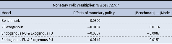
The results in Table 2 reveal that ignoring endogenous feedback may understate the impact of monetary policy in general. That is, the real effect of monetary policy is roughly twice as large when both types of uncertainties are treated as endogenous, compared to the case that closes the endogenous channel for both of them.
Next, we shut down the endogeneity channels one by one to separate the influences from each uncertainty. The third and fourth rows show that while endogenous feedback of real uncertainty strengthens the real effect of monetary policy, that of financial uncertainty turns out to weaken the efficacy of monetary policy. This result is straightforward when we combine the following two observations: a monetary tightening aggravates real uncertainty while it improves financial uncertainty and both real and financial uncertainty have negative impacts on real activity.
While monetary policy seems to be more potent when uncertainty is set to be endogenous, it is questionable whether the difference is significant. To this end, we compute the differences in the impact of monetary policy for possible solutions. Figure 4 shows the computed differences between environments with and without endogeneity in uncertainty over the identified set. The vertical dotted line is located at zero. If monetary policy is indeed more potent when endogeneity of uncertainty is introduced, then more mass should be concentrated on the right-hand side of the vertical line. Although there is a small possibility that monetary policy is more effective when the endogeneity channel is closed, the model produces more effective monetary policy when endogeneity is allowed more than 99% of the time. Hence, we can confidently conclude that the monetary policy effect might be underestimated when endogeneity of economic uncertainty is ignored.
Set of identified multipliers, Endogeneous vs. Exogeneous: The solid line represents the difference between the fully exogenous uncertainty case and the fully endogenous uncertainty case.
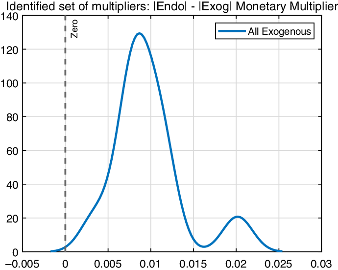
In sum, allowing endogenous channels may considerably affect the consequences of monetary policy. To be specific, endogenous feedback from real uncertainty strengthens the real effect of monetary policy, while that from financial uncertainty dampens the effect. Even though the two channels create tension as they affect real activity in opposite directions, feedback from real uncertainty outweighs that from financial uncertainty. This hints that it is important to understand the nature of uncertainty when conducting an empirical analysis of the impacts of uncertainty on the economy.
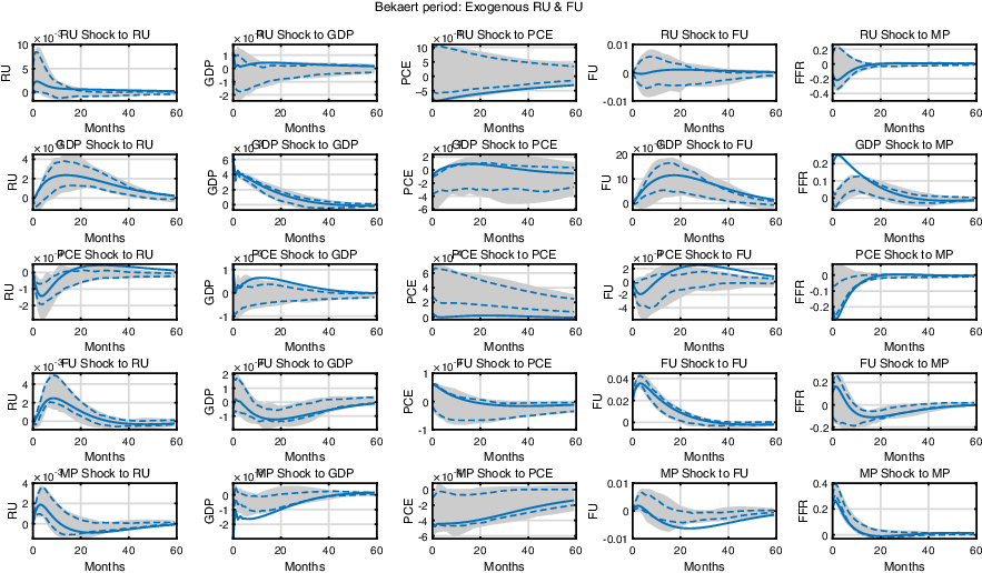
3.3 Comparison with Bekaert et al. (Reference Bekaert, Hoerova and Duca2013)
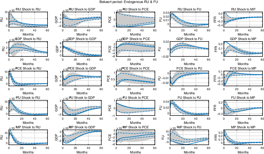
Previous literature that studied the impact of economic policy on uncertainty is limited. One exception is Bekaert et al. (Reference Bekaert, Hoerova and Duca2013) (BHL, henceforth), which examines the effects of monetary policy on uncertainty. In particular, they analyze how monetary policy affects risk appetite and uncertainty, and find that a lax monetary policy decreases uncertainty. In this subsection, we compare our results with those obtained in BHL. It is not appropriate to compare their results directly with ours, as they do not consider data after the GFC and they stop their sample in 2007. Hence, in this subsection we re-estimate the model using a shorter data sample that ends in December 2007, as used in BHL.
Figure 5 contains the baseline results with a shorter sample, excluding the period after the GFC. In this case, a tighter monetary policy still heightens real uncertainty while it lowers financial uncertainty. This result contradicts with the results derived in BHL, in which financial uncertainty is increasing in the monetary policy rate. It also suggests that the main result of this research is robust to the changes in the sample period.
Comparison with BHL. The impulse response functions of the monetary SVAR model through to Dec. 2007. The shaded area and the dashed lines represent the 90% and 68% confidence bands, respectively, and the solid lines represent the max-C impulse responses.
One additional difference between the two articles that may possibly contribute to this discrepancy in the results is the endogeneity of uncertainty in our model. In particular, financial uncertainty is exogenous in BHL while it is endogenous in ours, in the sense that the contemporaneous reactions of uncertainty to economic variables are allowed. Therefore, we conduct an analysis while shutting off the endogenous channel, as in Subsection 3.2. The results are summarized in Figure 6. Similar to the baseline results, a contractionary monetary policy shock increases real uncertainty. However, a tighter monetary policy increases financial uncertainty when the endogenous response channel is absent, which is similar to the result obtained in BHL. This exercise provides a possible explanation for the noticeably different results between this paper and BHL. To be precise, it suggests that the timing restriction used in BHL to identify the structural shocks may be too restrictive, for example, not allowing contemporaneous feedback between uncertainty and monetary policy, to identify the shocks related to uncertainties.
Comparison with BHL. The impulse response functions of the monetary SVAR model through to Dec. 2007 without the endogenous response of uncertainty. The shaded area and the dashed lines represent the 90% and 68% confidence bands, respectively, and the solid lines represent the median impulse responses.
4. Conclusion
In this research, we examine the nature of different types of uncertainty and analyze how monetary policy affects the level of both real and financial uncertainty. While the economic influence of uncertainty has been widely studied after Bloom (Reference Bloom2009), the economic forces that drive uncertainty have attracted relatively less attention. Specifically, while the role of uncertainty in shaping the effectiveness of monetary policy has been explored quite a lot, there has been little research that analyzes the impacts of monetary policy on economic uncertainty.
We find that monetary policy has a distinct effect on both real and financial uncertainty. In particular, it turns out that a tighter monetary policy dampens financial uncertainty, while injecting more uncertainty into the real sector. This result differs from the widely accepted belief that lax monetary action can stabilize financial uncertainty (Bekaert et al. (Reference Bekaert, Hoerova and Duca2013)) and bears important policy implications justifying an active monetary policy that targets financial stability.
In addition, we also show that accounting for the endogeneity of uncertainty does matter when analyzing the effects of monetary policy. Specifically, it is shown that implications regarding the behavior of uncertainties facing monetary policy action may alter if endogeneity is not properly taken into account. Furthermore, the impact of the monetary policy shock may be underestimated if the endogenous responses of the uncertainties are ignored in the policy analyses.
Supplementary material
To view supplementary material for this article, please visit http://doi.org/10.1017/S1365100523000111.
Acknowledgements
We thank the editor and two anonymous referees for constructive comments that substantially improved the manuscript. We are also grateful to Yoosoon Chang, Sangyup Choi, Soohyon Kim, Eunseong Ma, Joonseok Oh, Woong Yong Park, Serena Rhee, Donghoon Yoo, and seminar participants at the Bank of Korea, Korean Macro Research Group, and Korean Economic Review International Conference 2020 for their valuable suggestions. The views expressed IN this paper are solely those of the authors and do not necessarily reflect those of the Bank of Korea nor of the Korea Labor Institute. All errors are ours.


 Open access