2.1. The environment

We suppose that a stock of pollution, $E_{t+1}$ , is increased by consumption, $c_t$ , but reduced by mitigation, $m_t$ :

(1) \begin{eqnarray} E_{t+1}=(1-\delta _E)E_t+\epsilon c_t-\gamma m_t, \end{eqnarray}

where $\delta _E\in (0,1)$ measures a natural rate of pollution absorption. $\epsilon,\gamma \gt 0$ represent the rate of pollution from consumption and the efficiency of pollution abatement from mitigation, respectively.Footnote ¹

Pollution stock is a source of damage, resulting in climate change, frequent flooding, rising sea levels, and an increase in infectious diseases. However, damage can be alleviated through adaptation $H_{t+1}$ , such as dams, sea- or river-side banks, and medical knowledge. This could be public infrastructure or human capital. The adaptation stock is increased by public investment $h_t$ :

(2) \begin{eqnarray} H_{t+1} = \bar {H}+ (1 -\delta _H)H_t + h_t \end{eqnarray}

where $\bar {H}\gt 0$ is a basic (natural) adaptation level that nature provides and $\delta _H\in (0,1)$ denotes the rate of adaptation stock depreciation. Natural adaptation ( $\bar {H}$ ) is a long-term exogenous adaptation capacity that can be interpreted as the natural capacity of an ecosystem to protect humans. The higher the $\bar {H}$ , the more resistant the human being is to the hazards of nature, reflecting the low impact of pollution on well-being. $\bar {H}$ represents a natural long-term equilibrium (water, air, biodiversity, etc.) in the absence of any human activity.Footnote ²

Adaptation and mitigation investments play distinct roles. On the one hand, adaptation $h$ is an investment that increases a stock of public good, $H$ , financed by the government. On the other hand, mitigation $m$ is a privately provided good that decreases the pollution stock $E$ . With regard to climate change, $h$ is investment in infrastructure, education and R&D. $m$ is investment in GHG emission abatement services, such as CCS or renewable energy, and in the insulation of buildings.

2.2. Households

We consider an OLG model with 2-period-lived agents. The population size of each generation is assumed constant and normalized to unity. An individual born at time $t$ inelastically supplies one unit of labor when young, shares her wage between savings and investment in mitigation, $m_{t}$ , and consumes when old, $c_{t+1}$ . In addition, she suffers from a stock of pollution when old, $E_{t+1}$ , through climate change, sea level rise, or infectious diseases. However, vulnerability to environmental degradation is alleviated by a stock of adaptation, $H_{t+1}$ .

We define a sub-utility function, $q_{t+1}=Q(E_{t+1},H_{t+1})$ , which measures the quality of life related to the pollution stock. This quality is assumed to decrease with the pollution stock but increases with the adaptation stock. Together with consumption, we suppose that the utility of an individual born at time $t$ is

(3) \begin{eqnarray} u_t&=&c_{t+1}^\beta q_{t+1}^{1-\beta }, \end{eqnarray}

(4) \begin{eqnarray} q_{t+1}&=&E^{-\phi }_{t+1} H^\mu _{t+1}, \end{eqnarray}

where $\beta \in (0,1)$ is a preference parameter for consumption, $\phi \gt 0$ measures the sensitivity of quality of life to the pollution stock, and $\mu \gt 0$ is an efficiency parameter of the adaptation stock. $\phi$ can be interpreted as a parameter that determines the willingness to pay to reduce pollution or as a factor determining the share of mitigation expenditure in household income. $\mu$ can be interpreted as a vulnerability parameter, and $H^\mu$ represents the environmental resilience or the efficiency of adaptation to protect people from adverse climate change effects.

An individual born at time $t$ earns disposable income when young as the difference between wage $w_t$ , and lump-sum tax $T_t$ . She allocates this to mitigation $m_t$ and savings $s_t$ . When old, the agent consumes $(c_{t+1})$ her remunerated savings, with $R_{t+1}$ the real interest rate. The mitigation subsidy is $v$ , and the rate of consumption tax is $\tau _c$ . Thus, the individual maximizes (3) subject to (4) and (1) and the following budget constraints:

(5) \begin{eqnarray} (1-v)m_t+s_t&=&w_t-T_t, \end{eqnarray}

(6) \begin{eqnarray} (1+\tau ^c)c_{t+1}&=&R_{t+1}s_t. \end{eqnarray}

Households have to pay a tax $\tau ^c$ on polluting consumption (i.e., Pigovian tax). Their life-cycle income is also affected by a transfer $T_t$ (positive or negative) that balances the government budget. Households bear double taxation over their lifecycles ( $T$ and $\tau _c$ ). These two instruments are complementary, and allow us to define a complete system of instruments to decentralize the social optimum. The lump-sum tax has an impact on the level of life-cycle net income (scale effect), while the tax on consumption influences the pollution externalities from consumption.

Combining (5) and (6) leads to the intertemporal budget constraint.

\begin{eqnarray*} (1-v)m_t+\frac {1+\tau ^c}{R_{t+1}}c_{t+1}=w_t-T_t. \end{eqnarray*}

$H_{t+1}$ in (2) is given for agents. We derive the demand for mitigation when young, and consumption when old.

(7) \begin{eqnarray} m_t&=&\frac {w_t-T_t}{1-v}-\frac {\beta }{1-\beta }\frac {E_{t+1}}{\gamma \phi }, \end{eqnarray}

(8) \begin{eqnarray} c_{t+1}&=&\frac {R_{t+1}}{1+\tau ^c}\frac {\beta }{1-\beta }\frac {1-v}{\gamma \phi }E_{t+1}. \end{eqnarray}

The consequences of mitigation on the pollution stock are twofold. First, mitigation $m_t$ directly decreases the pollution stock $E_{t+1}$ . Second, higher investment in mitigation implies a decrease in individual savings and lower consumption in period $t+1$ . As adaptation is given, the vulnerability indicator does not influence agents’ trade-offs. Public adaptation has no direct consequence for the mitigation private decision.

2.3. Firms

The firm produces an aggregate output using a Cobb–Douglas technology with capital stock $K_t$ and labor $L_t$ : $Y_t =AK_t^\alpha L_t^{1-\alpha }$ with $A \gt 0$ and $\alpha \in (0,1)$ . Labor input equals one. We rewrite the production function as per capita $y_t = Ak_t$ , where $y_t$ and $k_t$ are the output and capital stock per young capita, respectively. The tax rate on production is $\tau ^y$ . This will affect the dynamics of capital accumulation.

The first-order conditions of profit maximization are given by

(9) \begin{eqnarray} R_{t}&=&(1-\tau ^y)\alpha Ak_t^{\alpha -1}, \end{eqnarray}

(10) \begin{eqnarray} w_t&=&(1-\tau ^y)(1-\alpha)Ak_t^\alpha \end{eqnarray}

We assume a full depreciation of capital in one period.

2.4. Government

The government’s budget is balanced at each period:

(11) \begin{eqnarray} T_t=vm_t+h_t-\tau ^c c_t -\tau ^y y_t. \end{eqnarray}

We first assume that investment in adaptation is constant over time, $h_t = \bar {h}$ , $\forall t$ . This investment is an environmental policy instrument. We therefore assume that adaptation is a choice made by independent local authorities and taken as given by central authorities in charge of taxation. We will relax this assumption later.

The distributive effects of adaptation and mitigation differ. The costs of environmental policies at time $t$ (investment in adaptation and mitigation subsidies) are borne by all agents living at time $t$ including old agents and firms, whereas the benefits will take place at time $t + 1$ . Mitigation is privately financed by the young at time $t$ for their own benefit when old at time $t + 1$ .

3.1. Laissez-faire equilibrium

We first consider the laissez-faire case ( $\tau ^c =\tau ^y = v = \bar {h} = 0$ ). Dynamics defined in eq. (16) reduces to

(17) \begin{eqnarray} k_{t+1}\equiv \Gamma _0(k_t)=\frac {\{1-\alpha (1+\epsilon /\gamma)\}\beta Ak_t^{\alpha }-\phi (1-\beta)(1-\delta _E)k_t}{\beta -(1-\beta)\phi }. \end{eqnarray}

We make the following assumptions to obtain the nontrivial steady state in the laissez-faire economy:

Assumption1 (a) compares the sensitivity of the quality of life to pollution ( $\phi$ ) to the sensitivity of utility to consumption ( $\beta$ ). Assumption1 (b) is standard and not too restrictive. This implies that $\gamma (1-\alpha)Ak^\alpha \gt \epsilon \alpha Ak^\alpha$ . In the absence of taxes, we have $c = Rs = Rk = \alpha Ak^\alpha$ and $w = (1 -\alpha) Ak^\alpha$ . Thus, the assumption is rewritten as $\gamma (1 -\alpha)w \gt \epsilon \alpha c$ , meaning that if an agent uses all her wages for mitigation ( $m = w$ ), it efficiently fights the flow of pollution from consumption, and then ensures that the flow of net pollution is negative.

Consequently, we have a positive denominator in (17) from assumption1 (a). Additionally, $\Gamma _0(0)=0$ , $\lim _{k_t\rightarrow 0} \Gamma _0^{\prime} (k_t)=+ \infty$ , and $\lim _{k_t\rightarrow +\infty } \Gamma _0^{\prime} (k_t)\lt 0$ .Footnote ³ Therefore, we obtain an inverted U-shaped curve in the dynamics of $k$ with an intercept at $k_{t+1}=0$ . Then, two steady states exist, such that $k=\Gamma _0(k)$ . Letting $k_{0,ss}^1$ and $k_{0,ss}^2$ be the capital stock levels at steady state, we have

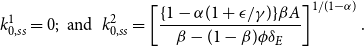\begin{eqnarray*} k_{0,ss}^1=0; & \mbox{ and } & k_{0,ss}^2=\left [ \frac {\{ 1-\alpha (1+\epsilon /\gamma)\}\beta A}{\beta -(1-\beta)\phi \delta _E} \right]^{1/(1-\alpha)}. \end{eqnarray*}

To examine the stability of each steady state, we define $\overline {k_0}$ as the capital stock that satisfies $\Gamma _0^{\prime}(\overline {k_0})=0$ and $\underline {k_0}$ as the stock satisfying $\Gamma _0^{\prime}(\underline {k_0})=-1$ . These are rewritten as

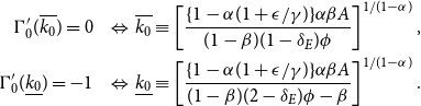\begin{eqnarray*} \Gamma _0^{\prime}(\overline {k_0})=0\;\;\; & \Leftrightarrow & \overline {k_0}\equiv \left [ \frac {\{ 1-\alpha (1+\epsilon /\gamma) \}\alpha \beta A}{(1-\beta)(1-\delta _E)\phi } \right]^{1/(1-\alpha)}, \\ \Gamma _0^{\prime}(\underline {k_0})=-1\;\;\; & \Leftrightarrow & \underline {k_0}\equiv \left [ \frac {\{ 1-\alpha (1+\epsilon /\gamma) \}\alpha \beta A}{(1-\beta)(2-\delta _E)\phi -\beta } \right]^{1/(1-\alpha)}. \end{eqnarray*}

From Assumption1, we obtain $k_{0,ss}^1\lt \overline {k_0}\lt \underline {k_0}$ . Then, we present three cases of dynamics: (i) $k_{0,ss}^1\lt \overline {k_0}\lt \underline {k_0}\le k_{0,ss}^2$ ; (ii) $k_{0,ss}^1\lt \overline {k_0}\lt k_{0,ss}^2\lt \underline {k_0}$ ; and (iii) $k_{0,ss}^1\lt k_{0,ss}^2\le \overline {k_0}\lt \underline {k_0}$ , which are depicted in Figure 1. As shown in Figure 1, the positive steady state $k_{0,ss}^2$ is unstable in case (i) and stable in cases (ii) and (iii).

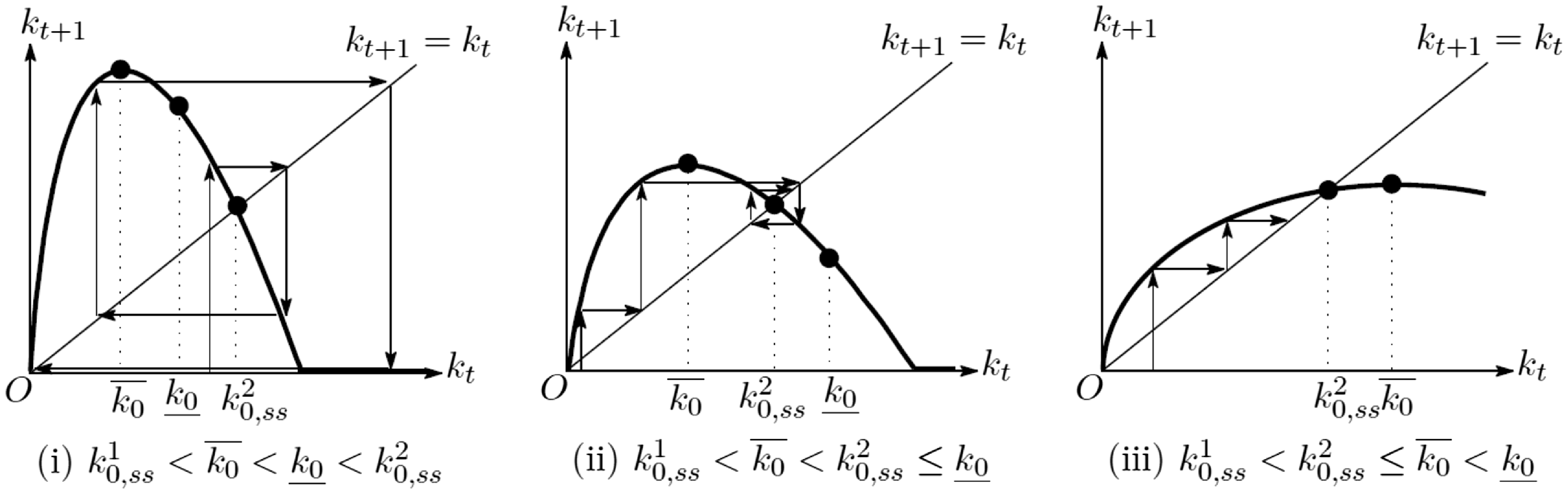
Figure 1. Capital stock dynamics in the laissez-faire economy.

We add the following assumption to ensure the existence of a nontrivial stable steady state in the laissez-faire cases, such as in cases (ii) and (iii). This is achieved by assuming $k_{0,ss}^2\lt \underline {k_0}$ , which is rearranged as follows:

This assumption also implies that utility is sufficiently sensitive to consumption.

3.2. Steady states with environmental policies

While holding Assumptions1 and 2, we study the dynamics of $k$ with policies, as in (13). We define $k_{ss}$ as the capital stock per young person if the steady state is unique, whereas $k_{ss}^i$ with $i=\{1,2,\cdots,n\}$ are those with $k^i_{ss}\lt k_{ss}^j$ for $i\lt j$ if there are multiple steady states.

Let us examine the steady-state capital stock. For this purpose, we define $\overline {k}$ , $\underline {k}$ , and $\hat {k}$ that satisfy $\Gamma ^{\prime}(\overline {k})=0$ , $\Gamma ^{\prime}(\underline {k})=-1$ , $\Gamma ^{\prime}(\hat {k})=1$ , respectively.

(18) \begin{eqnarray} \Gamma ^{\prime}(\overline {k})=0\;\;\; & \Leftrightarrow & \overline {k}\equiv \left [ \frac {(1-v)\left \{1-\alpha \frac {1-\tau ^y}{1+\tau ^c}(1+\epsilon /\gamma) \right \}\alpha \beta A}{\phi (1-\beta)(1-\delta _E)}\right]^{1/(1-\alpha)},\qquad\,\, \end{eqnarray}

(19) \begin{eqnarray} \Gamma ^{\prime}(\underline {k})=-1 & \Leftrightarrow & \underline {k}\equiv \left [ \frac {(1-v)\left \{1-\alpha \frac {1-\tau ^y}{1+\tau ^c}(1+\epsilon /\gamma) \right \}\alpha \beta A}{\phi (1-\beta)(1-\delta _E)+\{(1-\beta)\phi -(1-v)\beta \}}\right]^{1/(1-\alpha)}, \end{eqnarray}

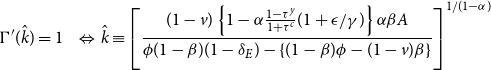(20) \begin{eqnarray} \Gamma ^{\prime}(\hat {k})=1 \;\;\; & \Leftrightarrow & \hat {k}\equiv \left [ \frac {(1-v)\left \{1-\alpha \frac {1-\tau ^y}{1+\tau ^c}(1+\epsilon /\gamma) \right \}\alpha \beta A}{\phi (1-\beta)(1-\delta _E)-\{(1-\beta)\phi -(1-v)\beta \}}\right]^{1/(1-\alpha)}\,\,\, \end{eqnarray}

We define two values for the mitigation subsidy, $\underline {v}$ and $\bar {v}$ , and summarize the existence and stability of the steady states as follows:

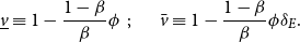(21) \begin{eqnarray} \underline {v}\equiv 1-\frac {1-\beta }{\beta }\phi \;\;; \;\;\;\;\;\;\;\; \bar {v}\equiv 1-\frac {1-\beta }{\beta }\phi \delta _E. \end{eqnarray}

Note that $\bar {v}\gt \underline {v}$ because $\delta _E\in (0,1)$ .

Additionally, from (16), we assume the following to exclude extreme cases:

Assuming that the subsidy rate is sufficiently high or low, we can characterize the steady-state equilibrium conditions. This highlights the importance of environmental policy tools. The level of mitigation subsidy determines the properties of the steady-state equilibrium and will also help determine the consequences of environmental tax and public finance reforms.

In the following section, we focus on the stable steady state.

3.3. Comparative statics

We evaluate the capital stock dynamics shown in (16) at the steady state by setting $k_{t+1}=k_{t}=k_{ss}$ . We then define the implicit function $I$ as

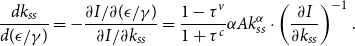
(22) \begin{eqnarray} I \equiv \left \{ 1-\alpha \frac {1-\tau ^y}{1+\tau ^c}(1+\epsilon /\gamma) \right \}Ak_{ss}^\alpha +\left \{ \frac {(1-\beta)\phi \delta _E}{(1-v)\beta }-1 \right \}k_{ss}-\bar {h}=0. \end{eqnarray}

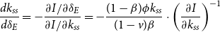
The implicit function theorem shows that

(23) \begin{eqnarray} \frac {d k_{ss}}{d \bar {h}}=-\frac {\partial I/\partial \bar {h}}{\partial I/\partial k_{ss}} =\left [ \left \{ 1-\alpha \frac {1-\tau ^y}{1+\tau ^c} (1+\epsilon /\gamma) \right \}\alpha A k_{ss}^{\alpha -1}+\left \{ \frac {(1-\beta)\phi \delta _E}{(1-v)\beta }-1 \right \} \right]^{-1}. \end{eqnarray}

From (23), $d k_{ss}/d \bar {h}$ is positive if

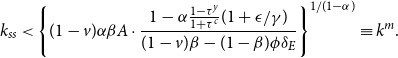(24) \begin{eqnarray} k_{ss}\lt \left \{ (1-v)\alpha \beta A\cdot \frac {1-\alpha \frac {1-\tau ^y}{1+\tau ^c}(1+\epsilon /\gamma)}{(1-v)\beta -(1-\beta)\phi \delta _E} \right \}^{1/(1-\alpha)}\equiv k^m. \end{eqnarray}

The numerator of $k^m$ is positive according to Assumption1(b). However, the denominator sign remains ambiguous. If $v\ge \bar {v}$ , then the set of capital stocks satisfying (24) is empty. That is, $dk_{ss}/d\bar {h}\lt 0$ if $v\ge \bar {v}$ . There is a range $[0,k^m)$ that is not empty if $v\lt \bar {v}$ . Then, we have $dk_{ss}/d\bar {h}\gt 0$ for $k_{ss}\in [0,k^m)$ , whereas $dk_{ss}/d\bar {h}\le 0$ for $k_{ss}\ge k^m$ . The discussion thus far is summarized in Proposition2.

$k_{ss}$ increases because the rise in public adaptation investment conditionally crowds out the private provision of mitigation services $m$ . Then, it allows for more savings when young, more consumption when old, and thereby more pollution, but with a lower effect on agent’s welfare since adaptation has also increased. Thus, when $v$ and $k_{ss}$ are weak, more adaptation is beneficial.

We also compute the effects of variations in the environmental regeneration rate. The effect is not so obvious a priori because if pollution absorption increases, the environment improves, and agents will lower their abatement and increase their consumption by saving more when young. However, these effects remain ambiguous.

\begin{eqnarray*} \frac {dk_{ss}}{d\delta _E}=-\frac {\partial I/\partial \delta _E}{\partial I/\partial k_{ss}}=-\frac {(1-\beta)\phi k_{ss}}{(1-v)\beta }\cdot \left (\frac {\partial I}{\partial k_{ss}}\right)^{-1} \end{eqnarray*}

From (22) and (23), we have $\mbox{sign}(dk_{ss}/d\delta _E)=\mbox{sign}( -dk_{ss}/d\bar {h})$ . Alternatively, we have $dl k_{ss}/d \delta _E \gt$ 0 if $k_{ss}\gt k^m$ . Similarly, the effects of the mitigation rate (abatement rate to pollution rate, $\epsilon /\gamma$ ) can be derived as

\begin{eqnarray*} \frac {dk_{ss}}{d(\epsilon /\gamma)}=-\frac {\partial I/\partial (\epsilon /\gamma)}{\partial I/\partial k_{ss}}= \frac {1-\tau ^v}{1+\tau ^c}\alpha Ak_{ss}^\alpha \cdot \left (\frac {\partial I}{\partial k_{ss}}\right)^{-1}. \end{eqnarray*}

We have $d k_{ss}/d(\epsilon /\gamma)\gt 0$ if $k_{ss}\lt k^m$ . If the ratio increases, then the conclusions are the same as those for $\bar {h}$ . That is, $(\epsilon /\gamma)$ increases steady-state capital stock if $k_{ss}$ is sufficiently low.

The effects of other policies on the steady-state capital stock level can also be derived.

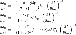\begin{eqnarray*} \frac {d k_{ss}}{dv} &=& -\frac {1-\beta }{\beta }\frac {\phi \delta _E}{(1-v)^2} k_{ss} \cdot \left (\frac {\partial I}{\partial k_{ss}}\right)^{-1},\\ \frac {d k_{ss}}{d\tau ^y} &=& -\frac {1+\epsilon /\gamma }{1+\tau ^c}\alpha Ak_{ss}^\alpha \cdot \left (\frac {\partial I}{\partial k_{ss}}\right)^{-1},\\ \frac {d k_{ss}}{d\tau ^c} &=& - \frac {1-\tau ^y}{(1+\tau ^c)^2}(1+\epsilon /\gamma)\alpha Ak_{ss}^\alpha \cdot \left (\frac {\partial I}{\partial k_{ss}}\right)^{-1} \end{eqnarray*}

These three derivatives are negative if $k_{ss}\lt k^m$ . The results are summarized below.

This result is interesting when we consider the heterogeneity between countries in terms of development and exposure to pollution. Indeed, the net effect of mitigation is all the more beneficial and significant the more developed the country (i.e., high per capita capital stock). Symmetrically, the lower the capital stock, the greater the risk that a low net mitigation efficiency rate will lead the country into decline. Indeed, the capital stock decreases in this ratio if the level of development is not sufficiently high.

From these results, we can assess the effect on consumption and mitigation at the steady state. Indeed, we have $c_{ss}=\frac {1-\tau ^y}{1+\tau ^c}\alpha Ak_{ss}^\alpha$ from (15). This implies that $c_{ss}$ evolves with $k_{ss}$ . This also depends on the tax variables.

The same results apply for $m_{ss}$ from (14), given as

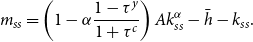(25) \begin{eqnarray} m_{ss}=\left ( 1-\alpha \frac {1-\tau ^y}{1+\tau ^c} \right) Ak_{ss}^\alpha -\bar {h}-k_{ss}. \end{eqnarray}

We show that the effects of public adaptation $\bar {h}$ on private mitigation $m_{ss}$ are ambiguous.

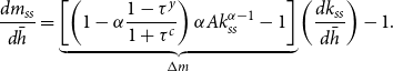(26) \begin{eqnarray} \frac {d m_{ss}}{d \bar {h}}=\underbrace {\left [ \left ( 1-\alpha \frac {1-\tau ^y}{1+\tau ^c} \right)\alpha Ak_{ss}^{\alpha -1}-1 \right]}_{\Delta m}\left (\frac {d k_{ss}}{d \bar {h}}\right)-1. \end{eqnarray}

The last term of (26), that is, −1, represents the resource-constraint effect of public adaptation. If the adaptation is increased, the income available to spend on mitigation reduces by the same proportion. By contrast, when adaptation increases the steady-state capital stock (i.e., the two terms in square brackets, $\Delta m$ ), it increases the current output, which leads to higher mitigation, whereas the increased savings lead to lower mitigation. Consequently, if the first term, $\Delta m\cdot \frac {dk_{ss}}{d\bar {h}}$ , is greater than unity, mitigation increases with adaptation.

However, because the sign of $\Delta m$ is ambiguous, we must examine it more closely. The term $\Delta m$ becomes positive if the increase in output is greater than the increase in savings. $\Delta m$ is positive if the capital stock in the steady state is sufficiently small such that

(27) \begin{eqnarray} k_{ss}\lt \left \{ \alpha A \left ( 1-\alpha \frac {1-\tau ^y}{1+\tau ^c} \right) \right \}^{1/(1-\alpha)}\equiv k^n. \end{eqnarray}

$k^n$ is positive for all $v$ and is greater than $k^m$ if $v\lt 1-\frac {1-\alpha \frac {1-\tau ^y}{1+\tau ^c}}{\alpha \frac {1-\tau ^y}{1+\tau ^c} \frac {\epsilon }{\gamma }} \frac {1-\beta }{\beta }\phi \delta _E\equiv \hat {v}$ . We have $\hat {v}\lt \bar {v}$ from Assumption1 (b).

As a result, mitigation and adaptation increase at the same time under certain conditions on the mitigation subsidy and capital stock level. Then, adaptation and mitigation are complements. The effect of $\bar {h}$ on $k_{ss}$ is very important in the transmission channels. The greater the effect, the stronger the complementarity. Otherwise, they are considered substitutes. Proposition3 summarizes this discussion.

Whether mitigation and adaptation are complementary or substitutionary depends, as already shown in the literature,Footnote ⁴ on the level of economic development ( $k$ ), but also on the accompanying environmental policy, namely, pollution taxation and mitigation subsidies. This last result is in line with the results of the work of Habla and Roeder (Reference Habla and Roeder2017).

4.1. The social optimum

First, we derive the optimal solution, which is the benchmark. Following Ono (Reference Ono1996), we suppose that the benevolent social planner treats all generations symmetrically. There is no intergenerational discounting and we assume that there exists a unique and stable long-term optimal allocation. The latter should guide public policy over the very long term, and thus help to determine the optimal instruments. Then, the problem is to maximize $u=c^\beta \cdot (E^{-\phi }\cdot H^{\mu })^{1-\beta }$ subject to $H=(\bar {H}+h)/\delta _H$ , $E=(\epsilon c -\gamma m)/\delta _E$ , and $Ak^\alpha =c+k+m+h$ .

By defining $A_0\equiv (\alpha A)^{1/1-\alpha }\frac {1-\alpha }{\alpha }$ , we can derive the optimal allocation as follows:

(28) \begin{align} k^*&=(\alpha A)^{\frac {1}{1-\alpha }}, \end{align}

(29) \begin{align} E^*&=\frac {\gamma }{\delta _E}\cdot \frac {\phi (1-\beta)}{\beta -(1-\beta)(\phi -\mu)}(A_0+\bar {H}),\end{align}

(30) \begin{align} m^*&= \frac {\epsilon \beta -\phi (1-\beta)(\gamma +\epsilon)}{\gamma +\epsilon }\cdot \frac {A_0+\bar {H}}{\beta -(1-\beta)(\phi -\mu)}, \end{align}

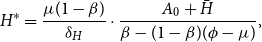
(31) \begin{align} h^*&=\frac {\mu (1-\beta)A_0-\{\beta -\phi (1-\beta)\}\bar {H}}{\beta -(1-\beta)(\phi -\mu)}, \end{align}

(32) \begin{align} H^*&=\frac {\mu (1-\beta)}{\delta _H}\cdot \frac {A_0+\bar {H}}{\beta -(1-\beta)(\phi -\mu)}, \end{align}

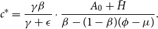(33) \begin{align} c^*&=\frac {\gamma \beta }{\gamma +\epsilon }\cdot \frac {A_0+\bar {H}}{\beta -(1-\beta)(\phi -\mu)}. \end{align}

To rule out trivial results, we assume the following parameter conditions:

This assumption implies a not too high natural stock of adaptation $\bar {H}$ . Under Assumption4, the optimal investment in adaptation $h^*$ in (31) decreases with the natural adaptation stock $\bar {H}$ . This is because natural adaptation increases the adaptation stock $H^*$ in (32) and decreases the marginal utility from the investment in adaptation. Conversely, natural adaptation, $\bar {H}$ , increases investment in mitigation, $m^*$ in (30), and consumption, $c^*$ in (33). The mechanism is as follows: Natural adaptation, $\bar {H}$ , decreases $h^*$ , whereas it has no effect on the capital stock level, $k^*$ in (28). The saved investment in $h^*$ thus increases $c^*$ and $m^*$ via the resource constraint. We also note that any increase in natural adaptation increase the optimal level of the pollution stock, $E^*$ in (29), as increased natural adaptation decreases the effect on utility from pollution emissions. In addition, following the increase in natural adaptation, the increase in emissions due to increased consumption is greater than the decrease in emissions due to the increase in mitigation; the stock of pollutants increases, that is, $\epsilon \cdot (\partial c^*/\partial \bar {H})\gt \gamma \cdot (\partial m^*/\partial \bar {H})$ hence, $(\partial E^*/\partial \bar {H})\gt 0$ .

The optimal mix between mitigation and adaptation can besummarized by the ratio $(m^*/h^*)$ :

(34) \begin{eqnarray} \frac {m^*}{h^*}=\frac {\frac {\epsilon \beta }{\gamma +\epsilon }-\phi (1-\beta)}{\mu (1-\beta)A_0-\beta \bar {H}+(1-\beta)\phi \bar {H}}(A_0+\bar {H}). \end{eqnarray}

We can easily observe that this ratio decreases with $\mu$ , $\phi$ , and $\gamma /\epsilon$ . That is, when the effects on utility from adaptation and pollution become greater ( $\mu$ and $\phi$ ), adaptation should be increased, rather than mitigation. Furthermore, even when mitigation efficiency is higher, adaptation is increased more than mitigation in the optimal policy plan.

4.2. Optimal policy schemes

The economy is characterized by four inefficiencies: dynamic inefficiency, pollution externality, public provision of adaptation, and private contribution to mitigation (Ono, Reference Ono1996). We need to determine the optimal values of the policy instruments, that is, $\tau ^c$ , $\bar {h}$ , $\tau ^y$ , and $v$ : (i) $c_{ss}/E_{ss}=c^*/E^*$ , (ii) $\bar {h}=h^*$ , (iii) $m_{ss}=m^*$ , and (iv) $k_{ss}=k^*$ .

First, we derive $\tau ^c(\tau ^y,v)$ from (i), which satisfies:

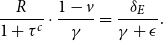(35) \begin{eqnarray} \frac {R}{1+\tau ^c}\cdot \frac {1-v}{\gamma }=\frac {\delta _E}{\gamma +\epsilon }. \end{eqnarray}

Second, we set the adaptation $\bar {h}$ directly from (ii) as $\bar {h}=h^*$ in (31). Third, mitigation satisfies (iii) by setting $v(\tau ^y,\tau ^c)$ which equalizes the following:

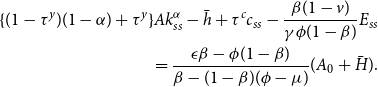(36) \begin{eqnarray} \{(1-\tau ^y)(1-\alpha)+\tau ^y\}Ak_{ss}^\alpha -\bar {h}+\tau ^c c_{ss}-\frac {\beta (1-v)}{\gamma \phi (1-\beta)}E_{ss}\nonumber \\ =\frac {\epsilon \beta -\phi (1-\beta)}{\beta -(1-\beta)(\phi -\mu)}(A_0+\bar {H}). \end{eqnarray}

Finally, $\tau _y$ is set to derive (iv). Given that $(1+\tau ^c)c_{ss}=R_{ss}s_{ss}$ from (6), $R_ss=(1-\tau ^y)\alpha k_{ss}^{\alpha -1}$ from (9), and the law of motion in the capital market is $k_{ss}=s_{ss}$ , we can describe $\tau ^y$ such that

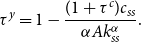(37) \begin{eqnarray} \tau ^y=1-\frac {(1+\tau ^c)c_{ss}}{\alpha A k^\alpha _{ss}}. \end{eqnarray}

From the discussion in this subsection, we obtain the following proposition.

4.3. Numerical simulation

To illustrate how the model performs, this section reports the results from some simple numerical examples. We show that the economy can converge towards a unique and stable long-run steady-state, and that a stable social optimum exists. The objective is also to show that assumptions1 to 4 for the existence and stability of steady-states can be satisfied simultaneously, for reasonable parameter values. We limit our simulations on cases where a non-zero steady-state exists (case (iii) with a sufficiently high mitigation subsidy and case (ix) with a low one).

We set the values of the parameters $\left \{ \beta,\alpha,\phi,\gamma,\epsilon,\delta _{E}\right \}$ using the estimates usually found in the literature on applied models, and in order to comply with the conditions imposed by assumptions $1$ to $4$ . To select the environmental parameters we used Bonen et al. (Reference Bonen, Loungani, Semmler and Koch2016) for guidance. We also followed Catalano et al. (Reference Catalano, Forni and Pezzolla2020a, b) and Fried et al. (Reference Fried, Novan and Peterman2018) in order to maintain comparability with other life-cycle studies. The rest of the parameters are reasonably standard within the life-cycle literature. We choose the values for the exogenous parameters as shown in Table 1.

Table 1. Parameter values

Concerning assumption about the consequences of adaptation, it is difficult to make comparisons with assumptions and results from other models.

Indeed, we assume that adaptation helps limit the effects of pollution on welfare, which is a subjective consequence. Empirical studies assessing the consequences of adaptation generally focus on objective physical indicators such as mortality risk (Carleton et al. Reference Carleton, Jina, Delgado, Greenstone, Houser, Hsiang, Hultgren, Kopp, McCusker, Nath, Rising, Rode, Seo, Viaene, Yuan and Zhang2022), agricultural yield (Hultgren et al. Reference Hultgren, Carleton, Delgado, Gergel, Greenstone, Houser, Hsiang, Jina, Kopp, Malevich, McCusker, Mayer, Nath, Rising, Rode and Yuan2022), factor productivity (Catalano et al. Reference Catalano, Forni and Pezzolla2020a, Reference Catalano, Forni and Pezzollab) or factor mobility (like migration). On the other hand, Bonen et al. (Reference Bonen, Loungani, Semmler and Koch2016) considers transmission channels for adaptation expenditure relatively close to our assumptions. Bonen et al. (Reference Bonen, Loungani, Semmler and Koch2016) introduces adaptation expenditure into the utility function, but as a flow of public expenditure and not as a stock of infrastructure or knowledge for adaptation. They assume a value for the elasticity of public capital used for adaptation in utility equal to 0.05, whereas we consider a value of 0.09, but for the impact of the adaptation stock.

First, we calculate the social optimal values, which depend only on technological ( $A,\alpha$ ) and environmental ( $\gamma,\epsilon,\bar {H},\delta _{H},\delta _{E}$ ) parameters and preferences ( $\beta,\phi,\mu$ ). As a benchmark, we obtain the optimal level of adaptation expenditure ( $h$ ) equal to 0.04. Then, we evaluate steady-states under different scenarios relating to budget spending. We present two alternative scenarios: in Table 2, the subsidy to mitigation $v$ is low (equal to 0), while in Table 3, the subsidy is high ( $v=0.9$ ). We add to these two policies decisions where the government engages in over- (resp. under-) spending on adaptation ( $\bar {h}=0.15\gt h^{\ast }$ resp. $\bar {h}=0.029\lt h^{\ast }$ ). These policies are combined with two tax schemes: laissez-faire $\tau ^{y}=\tau ^{c}=0$ and taxation with $\tau ^{y}=0.2$ and $\tau ^{c}=0.1$ .

Table 2. Low mitigation subsidy ( $v=0$ )

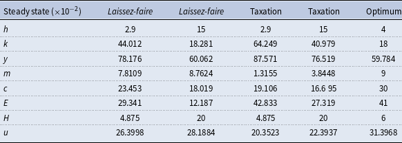
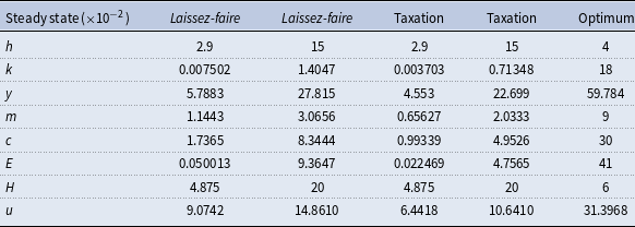
Table 3. High mitigation subsidy ( $v=0.9$ )

A first important result is that the level of subsidy $v$ significantly determines capital intensity at steady state. When the subsidy is low (Table 2), the economy is in a situation of capital over-accumulation, whereas a high subsidy (Table 3) causes capital to fall drastically, and the economy is then characterized by under-accumulation. We confirm the results in Proposition2. The increase in expenditure on adaptation ( $\bar {h}$ increases from 0.029 to 0.15) reduces the capital stock per capita in a situation of over-accumulation. Conversely, in a situation of under-accumulation, the rise in $\bar {h}$ increases $k$ . In both cases, adaptation is beneficial in terms of well-being because $k$ moves closer to its optimum value. More generally, any increase in the subsidy $v$ worsens the capital stock per capita, whatever the adaptation effort.

A second significant result relates to the impact on mitigation $m$ chosen by households. Private spending on mitigation has a twofold impact on pollution. A direct effect is to reduce the stock of pollution through the accumulation of pollutants, and an indirect effect is to reduce savings and hence consumption, the sole source of pollution. When the subsidy to mitigation is low (Table 2), the increase in $m$ is accompanied by a reduction in economic activity, consumption and therefore pollution. This situation is pareto-improving because the economy is over-accumulating capital. On the other hand, when the subsidy is high (Table 3), the opposite mechanisms are at work, since the increase in $m$ goes hand in hand with an increase in $k,c$ and therefore $E$ . In this case too, these changes are beneficial in terms of welfare despite the rise in pollution. Indeed, the increase in $m,c$ and $k$ follows an increase in $\bar {h}$ : households consume more and are better protected against pollution. In this example, we show that any increase in $\bar {h}$ leads to an increase in $m$ , whatever the tax scheme ( $v,\tau ^{y},\tau ^{c}$ ). We are therefore in a situation where adaptation and mitigation are complements (see Proposition3).

We find the results of corollary1 on the impact of instruments (i.e., laissez-faire vs taxation) on the capital stock per capita. When the latter is high (i.e., $v$ low, Table 2), higher taxes increase the capital stock, whereas the effect is negative when the capital stock is low (Table 3).

When the mitigation subsidy is small (Table 2), the level of mitigation is low (relative to the optimum), and counter-intuitively, the level of pollution is also small. This result can be explained by the high level of the capital stock per capita, which absorbs the greater part of the production of goods, and which does not pollute, unlike consumption. This effect is even stronger when expenditure on adaptation is high ( $\bar {h} =0.15$ ), reflecting a substitution between consumption and adaptation to the environment. As a result, welfare increases. Note that when the mitigation subsidy is high, private mitigation choices and capital per capita are highly sensitive to public decisions on adaptation ( $\bar {h}$ ).

5.1. Proportional adaptation

We suppose a case in which the adaptation level is determined by the flow of pollutants. This implies that, in a sense, mitigation influences adaptation. Hence, if mitigation increases, it implies a lower consumption level (budget constraint) and adaptation level. We extend the previous results to the case where the investment in adaptation is set proportionally to the flow of pollution at a constant rate $z\ge 0$ :

(38) \begin{eqnarray} h_t=z\cdot \epsilon c_t. \end{eqnarray}

This policy implies a relationship between the current adaptation $h_t$ and previous mitigation $m_{t-1}$ . Indeed, $h_t$ must increase if consumption $c_t$ increases. This is possible if savings $s_{t-1}$ increases and mitigation $m_{t-1}$ decreases, ceteris paribus.

By substituting (38) into (11) and using (8), (9), and (12), the dynamics of capital stock per young are given by

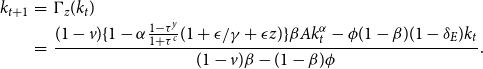(39) \begin{eqnarray} k_{t+1}&=&\Gamma _z(k_t)\nonumber \\ &=&\frac {(1-v)\{1-\alpha \frac {1-\tau ^y}{1+\tau ^c}(1+\epsilon /\gamma +\epsilon z) \}\beta Ak_t^\alpha - \phi (1-\beta)(1-\delta _E)k_t}{(1-v)\beta - (1-\beta)\phi }. \end{eqnarray}

In this case, we have two steady states with $k^1_{ss}$ and $k^2_{ss}$ such that

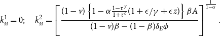(40) \begin{eqnarray} k^1_{ss}=0; \;\;\;\;\;\; k^2_{ss}=\left [ \frac {(1-v)\left \{ 1-\alpha \frac {1-\tau ^y}{1+\tau ^c}(1+\epsilon /\gamma +\epsilon z) \right \} \beta A}{(1-v)\beta -(1-\beta)\delta _E\phi }\right]^{\frac {1}{1-\alpha }}. \end{eqnarray}

Let us consider the conditions for positive capital stock in a non-trivial steady state, $k_{ss}^2\gt 0$ . This is easily attained by assuming that $\frac {1-\alpha \frac {1-\tau ^y}{1+\tau ^c}(1+\epsilon /\gamma +\epsilon z)}{(1-v)\beta -(1-\beta)\delta _E\phi }\gt 0.$ On the one hand, the denominator becomes negative (resp. positive) if the mitigation subsidy is greater than $\bar {v}$ (resp. lower than $\bar {v}$ ). On the other hand, the numerator can also be negative (resp. positive) if the adaptation provision rate $z$ is greater than $\bar {z}$ (resp. lower than $\bar {z}$ ), as defined below.

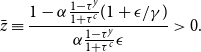(41) \begin{eqnarray} \bar {z}\equiv \frac {1-\alpha \frac {1-\tau ^y}{1+\tau ^c}(1+\epsilon /\gamma)}{\alpha \frac {1-\tau ^y}{1+\tau ^c}\epsilon }\gt 0. \end{eqnarray}

From Assumption1(b), $\bar {z}$ is positive. For the nontrivial steady state with $k_{ss}^2$ , we suppose that the environmental policy tools satisfy the following:

This assumption requires either sufficiently large or sufficiently small mitigation and adaptation. We therefore exclude intermediate cross-cases in order to restrict the analysis to situations where there exist two stationary states with at least one non-trivial stable steady state.

To examine the stability of the steady state, we define $\overline {k_z}$ , $\underline {k_z}$ , and $\hat {k_z}$ as follows.

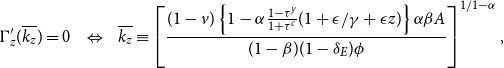(42) \begin{eqnarray} \Gamma _z^{\prime}(\overline {k_z})=0 \;\;\; &\Leftrightarrow & \;\;\; \overline {k_z}\equiv \left [ \frac {(1-v)\left \{ 1-\alpha \frac {1-\tau ^y}{1+\tau ^c}(1+\epsilon /\gamma +\epsilon z) \right \}\alpha \beta A}{(1-\beta)(1-\delta _E)\phi } \right]^{1/1-\alpha }, \end{eqnarray}

(43) \begin{eqnarray} \Gamma _z^{\prime}(\underline {k_z})=-1 \;\;\; &\Leftrightarrow & \;\;\; \underline {k_z}\equiv \left [ \frac {(1-v)\left \{ 1-\alpha \frac {1-\tau ^y}{1+\tau ^c}(1+\epsilon /\gamma +\epsilon z) \right \}\alpha \beta A}{(1-\beta)(2-\delta _E)\phi -(1-v)\beta } \right]^{1/1-\alpha }, \end{eqnarray}

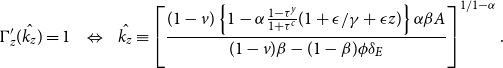(44) \begin{eqnarray} \Gamma _z^{\prime}(\hat {k_z})=1 \;\;\; &\Leftrightarrow & \;\;\; \hat {k_z}\equiv \left [ \frac {(1-v)\left \{ 1-\alpha \frac {1-\tau ^y}{1+\tau ^c}(1+\epsilon /\gamma +\epsilon z) \right \}\alpha \beta A}{(1-v)\beta -(1-\beta)\phi \delta _E} \right]^{1/1-\alpha }. \end{eqnarray}

Consequently, from (39), Proposition5 characterizes the steady-state equilibrium with proportional adaptation.

As well as Proposition1, the mitigation subsidy is a key to the analysis of the dynamics of the capital stock. Depending on whether the subsidy is low or high enough, three cases for each exist. However, as the adaptation level is not fixed in this case, the analysis of the capital stock dynamics is simplified.

From this proposition, we focus on the steady state with $k_{ss}^2$ in cases (i) and (ii) of Proposition5. The nontrivial steady-state equilibrium is described as follows:

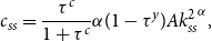(45) \begin{align} c_{ss}&=\frac {\tau ^c}{1+\tau ^c}\alpha (1-\tau ^y)A{k_{ss}^2}^\alpha, \end{align}

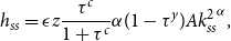(46) \begin{align} h_{ss}&=\epsilon z \frac {\tau ^c}{1+\tau ^c}\alpha (1-\tau ^y)A{k_{ss}^2}^\alpha, \end{align}

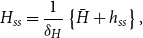(47) \begin{align} H_{ss}&=\frac {1}{\delta _H}\left \{ \bar {H}+h_{ss} \right \}, \end{align}

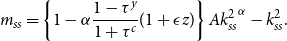(48) \begin{align} m_{ss}&=\left \{ 1-\alpha \frac {1-\tau ^y}{1+\tau ^c}(1+\epsilon z) \right \}A{k_{ss}^2}^{\alpha }-k_{ss}^2. \end{align}

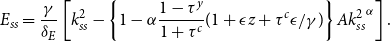(49) \begin{align} E_{ss}&= \frac {\gamma }{\delta _E}\left [ k_{ss}^2-\left \{ 1-\alpha \frac {1-\tau ^y}{1+\tau ^c}(1+\epsilon z+ \tau ^c \epsilon /\gamma) \right \} A{k_{ss}^2}^\alpha \right]. \end{align}

Next, we derive the derivatives of $k_{ss}^2$ with respect to the policy variables as a comparative statics study.

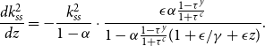(50) \begin{align} \frac {dk^2_{ss}}{dz}&=-\frac {k_{ss}^2}{1-\alpha }\cdot \frac {\epsilon \alpha \frac {1-\tau ^y}{1+\tau ^c}}{1-\alpha \frac {1-\tau ^y}{1+\tau ^c}(1+\epsilon /\gamma +\epsilon z)}. \end{align}

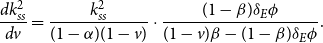(51) \begin{align} \frac {dk^2_{ss}}{dv}&=\frac {k_{ss}^2}{(1-\alpha)(1-v)}\cdot \frac {(1-\beta)\delta _E\phi }{(1-v)\beta -(1-\beta)\delta _E\phi }. \end{align}

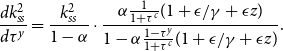(52) \begin{align} \frac {dk^2_{ss}}{d\tau ^y}&=\frac {k_{ss}^2}{1-\alpha }\cdot \frac { \alpha \frac {1}{1+\tau ^c}(1+\epsilon /\gamma +\epsilon z)}{1-\alpha \frac {1-\tau ^y}{1+\tau ^c}(1+\epsilon /\gamma +\epsilon z)}. \end{align}

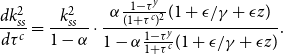(53) \begin{align} \frac {dk^2_{ss}}{d\tau ^c}&= \frac {k_{ss}^2}{1-\alpha }\cdot \frac { \alpha \frac {1-\tau ^y}{(1+\tau ^c)^2}(1+\epsilon /\gamma +\epsilon z)}{1-\alpha \frac {1-\tau ^y}{1+\tau ^c}(1+\epsilon /\gamma +\epsilon z)}. \end{align}

From (50)–(53), we immediately obtain the following corollary.

This corollary shows that capital stock does not always increase with the adaptation rate $z$ . This also implies, together with (45) and (47), that the adaptation rate, $z$ , does not always increase the adaptation flow, $h_{ss}$ , or the adaptation stock, $H_{ss}$ , in the steady state. To observe this in detail, we have from (46):

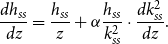\begin{eqnarray*} \frac {dh_{ss}}{dz}=\frac {h_{ss}}{z}+\alpha \frac {h_{ss}}{k_{ss}^2}\cdot \frac {dk_{ss}^2}{dz}. \end{eqnarray*}

The first term is a direct increase in $z$ whereas the second is an indirect increase via $k_{ss}^2$ . We define the fiscal scheme in (38). If $z$ decreases the capital stock, the consumption shown in (45) decreases, and thus the indirect effect decreases the adaptation flow and stock. We can rearrange this expression using (46) and (50) as:

(54) \begin{eqnarray} \frac {dh_{ss}}{dz}=\frac {\epsilon \frac {\alpha }{1-\alpha }\frac {1-\tau ^y}{1+\tau ^c}}{1-\alpha \frac {1-\tau ^y}{1+\tau ^c}(1+\epsilon /\gamma +\epsilon z)}\cdot (1-\alpha)\left \{ 1-\alpha \frac {1-\tau ^y}{1+\tau ^c}\left (1+\frac {\epsilon }{\gamma }+\frac {\epsilon z}{1-\alpha }\right)\right \}\tau ^c A{k_{ss}^2}^\alpha. \end{eqnarray}

We define $\underline {z}$ , which satisfies $\frac {dh_{ss}}{dz}=0$ :

(55) \begin{eqnarray} \underline {z}\equiv (1-\alpha)\bar {z}. \end{eqnarray}

Therefore, the derivative in (54) is strictly positive for $z\lt \underline {z}$ and strictly negative for $z\gt \underline {z}$ . Likewise, the effect on mitigation from the adaptation rate is ambiguous, as shown in (48):

(56) \begin{eqnarray} \frac {dm_{ss}}{dz}=\frac {\epsilon \frac {\alpha }{1-\alpha } \frac {1-\tau ^y}{1+\tau ^c}}{1-\alpha \frac {1-\tau ^y}{1+\tau ^c}(1+\epsilon /\gamma +\epsilon z)}\cdot \left [ \left \{ 1-\alpha \frac {1-\tau ^y}{1+\tau ^c}\left ( 1+(1-\alpha)\frac {\epsilon }{\gamma }+\epsilon z \right) \right \}A{k_{ss}^2}^\alpha -k_{ss}^2 \right]. \quad\,\end{eqnarray}

From (54) and (56), we obtain the following expression.

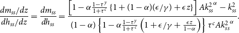(57) \begin{eqnarray} \frac {dm_{ss}/dz}{dh_{ss}/dz}=\frac {dm_{ss}}{dh_{ss}}=\frac {\left [ 1-\alpha \frac {1-\tau ^y}{1+\tau ^c}\left \{ 1+(1-\alpha)(\epsilon /\gamma)+\epsilon z \right \} \right]A{k_{ss}^2}^\alpha -k_{ss}^2}{ (1-\alpha)\left \{ 1-\alpha \frac {1-\tau ^y}{1+\tau ^c}\left ( 1+\epsilon /\gamma +\frac {\epsilon z}{1-\alpha } \right) \right \}\tau ^c A {k_{ss}^2}^\alpha }. \end{eqnarray}

The denominator becomes positive if $z\lt \underline {z}$ , whereas the square brackets of the numerator become positive if $z\lt \hat {z}$ defined as

(58) \begin{eqnarray} \hat {z}\equiv \bar {z}+\frac {\alpha }{\gamma }. \end{eqnarray}

Then, we have $\underline {z}\lt \bar {z}\lt \hat {z}$ . In addition to the adaptation rate, the numerator also has a threshold $k^\ell$ that determines its sign.

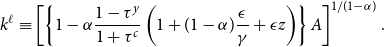(59) \begin{eqnarray} k^\ell \equiv \left [ \left \{ 1-\alpha \frac {1-\tau ^y}{1+\tau ^c}\left ( 1+ (1-\alpha)\frac {\epsilon }{\gamma }+\epsilon z \right) \right \}A \right]^{1/(1-\alpha)}. \end{eqnarray}

From the discussion thus far, the substitutability between mitigation and adaptation can be summarized as follows:

In the case of constant adaptation investment, mitigation and adaptation can be both complements and substitutes, but this depends on the adaptation rate and capital stock level at the steady state.

5.2. Public debt financing of adaptation

Results thus far assume that public investment in adaptation and mitigation subsidies is financed by taxes on current generations. However, as adaptation is a stock or durable good, it benefits not only the present generations but also future generations. Debt is an instrument that affects intertemporal transfers and intergenerational welfare. We assume that investment in adaptation is partly financed by public debt. This financing policy allows future generations to benefit from the accumulated adaptation stock and partly bear its present cost.

In particular, we suppose that adaptation investment is set at an optimal level at steady state and is totally financed by debt issuing. We focus on equilibria with constant debt per capita, that is, $B_t=B\gt 0$ for all $t\gt 0$ . Debt is constant so that steady-states can be explicitly determined. We consider public debt as an instrument of environmental policy, it finances investments in the adaptation stock. This instrument replaces the production tax. Optimal debt helps to achieve the optimal level of adaptation, as defined by (30) and (31), by substituting $h^*$ into $\bar {h}$ . Thus, the government budget is given as

(60) \begin{eqnarray} B=R_tB+\bar {h}-T_t-\tau ^c c_t+vm_t. \end{eqnarray}

We have the following capital market equilibrium:

(61) \begin{eqnarray} k_{t+1}=s_t-B. \end{eqnarray}

Eq. (61) is rewritten as the dynamics of capital stock:

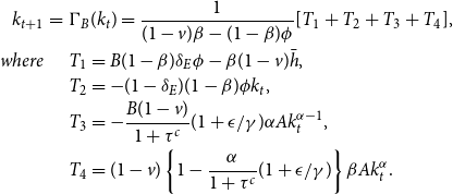(62) \begin{eqnarray} k_{t+1}&=&\Gamma _B(k_t)=\frac {1}{(1-v)\beta -(1-\beta)\phi }[T_1+T_2+T_3+T_4],\\ where&&T_1=B (1-\beta)\delta _E \phi - \beta (1-v)\bar {h},\nonumber \\ &&T_2= -(1-\delta _E)(1-\beta)\phi k_t,\nonumber \\ &&T_3= -\frac {B(1-v)}{1+\tau ^c}(1+\epsilon /\gamma)\alpha A k_t^{\alpha -1},\nonumber \\ &&T_4= (1-v)\left \{ 1-\frac {\alpha }{1+\tau ^c}(1+\epsilon /\gamma) \right \}\beta A k_t^\alpha.\nonumber \end{eqnarray}

With this expression, we obtain the following proposition for the steady-state equilibrium. For stability, we derive the derivatives of (62) as

(63) \begin{align} \Gamma _B^{\prime}(k_t)&=\frac {1}{(1-v)\beta -(1-\beta)\phi }\left [ -(1-\delta _E)(1-\beta)\phi +B\frac {1-v}{1+\tau ^c}(1-\alpha)(1+\epsilon /\gamma)\alpha Ak_t^{\alpha -2} \right.\nonumber \\ & \quad \left. +(1-v)\left \{ 1-\frac {\alpha }{1+\tau ^c}(1+\epsilon /\gamma) \right \}\alpha \beta A k_t^{\alpha -1} \right]. \end{align}

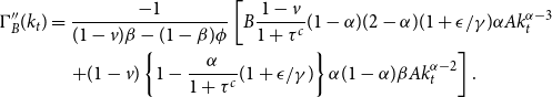(64) \begin{align} \Gamma _B^{\prime\prime}(k_t)&=\frac {-1}{(1-v)\beta -(1-\beta)\phi }\left [ B\frac {1-v}{1+\tau ^c}(1-\alpha)(2-\alpha)(1+\epsilon /\gamma)\alpha Ak_t^{\alpha -3} \right. \nonumber \\ & \quad \left. +(1-v)\left \{ 1-\frac {\alpha }{1+\tau ^c}(1+\epsilon /\gamma) \right \}\alpha (1-\alpha)\beta A k_t^{\alpha -2} \right]. \end{align}

Furthermore, to summarize the stability conditions, we define $\underline {k_B}$ , $\overline {k_B}$ , and $\hat {k_B}$ as $\Gamma _B^{\prime}(\underline {k_B})=-1$ , $\Gamma _B^{\prime}(\overline {k_B})=0$ , and $\Gamma _B^{\prime}(\hat {k_B})=1$ . These three levels are unique because (64) exhibits monotonicity of $\Gamma _B^{\prime}(k_t)$ .

As well as the previous models and as shown in Proposition1 and 5, the capital stock dynamics has two cases, depending on the subsidy rates. For each case, the dynamics have further three cases, depending on the capital stock.

From Proposition7, in the presence of a constant adaptation financed partly by debt, we focus on the locally stable nontrivial steady state, such as $k_{ss}^3$ in Case (iii) with $k_{ss}^3\lt \underline {k_B}$ and $k_{ss}^1$ in Case (vi) with $k_{ss}^1\gt \underline {k_B}$ .

We then develop comparative statics with respect to debt. By differentiating $\Gamma _B(k_t)$ with respect to the constant debt $B$ , we haveFootnote ⁵

(65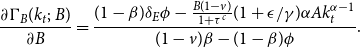) \begin{eqnarray} \frac {\partial \Gamma _B(k_t;\, B)}{\partial B}=\frac {(1-\beta)\delta _E\phi -\frac {B(1-v)}{1+\tau ^c}(1+\epsilon /\gamma)\alpha A k_t^{\alpha -1}}{(1-v)\beta -(1-\beta)\phi }. \end{eqnarray}

This implies that if $v\lt \underline {v}$ , the dynamics of the capital stock shift upward for $k_t\gt k^o$ and downwards for $k_t\lt k^o$ , where

(66) \begin{eqnarray} k^o\equiv \left \{\frac {B(1-v)(1+\epsilon /\gamma)\alpha A}{(1+\tau ^c)(1-\beta)\delta _E\phi }\right \}^{1/(1-\alpha)}. \end{eqnarray}

Because $B$ can take zero or larger values, $k^o$ can also take a wide range of values. By contrast, if $v\gt \underline {v}$ , the dynamics shift upward if $k_t\lt k^o$ and downward if $k_t\gt k^o$ .

Given this result, we consider the steady-state effect of debt. For this purpose, we suppose locally stable steady states. First, suppose $v\lt \underline {v}$ , $\Gamma _B(\hat {k_B})\gt \hat {k_B}$ , and $k_{ss}^3\lt \underline {k_B}$ , as in case (iii) of Proposition7. Then, steady-state capital stock $k_{ss}^3$ is locally stable. Suppose further that the economy lies on $k_{ss}=k_{ss}^3$ ; if $k_{ss}^3\gt k^o$ , a marginal increase in the constant debt to finance the constant adaptation increases the capital stock. Conversely, if $k_{ss}^3\lt k^o$ , debt decreases it. On the contrary, suppose $v\gt \underline {v}$ , $\Gamma _B(\hat {k_B})\lt \hat {k_B}$ , and $k_{ss}^1\gt \underline {k_B}$ as in case (vi) of Proposition7. Then, steady-state capital stock $k_{ss}^1$ is locally stable. Suppose further that the economy lies on $k_{ss}=k_{ss}^1$ ; if $k_{ss}^1\lt k^o$ , the debt increases the capital stock. If $k_{ss}^1\gt k^o$ , the debt decreases it.

We can summarize the results thus far in the following corollary.

Corollary3 says that when $B$ is sufficiently low, the initial capital stocks tend to be characterized by under-accumulation in both cases (i) and (ii). Then, an increase in public debt $B$ is welfare improving if it leads to an increase in the capital stock. When the government increases $B$ and thereby the adaptation, there are two opposing effects on $k$ . Any improvement in adaptation should reduce the need for mitigation (substitution effect), and thus increase savings. At the same time, public debt is increasing, which could lead to a crowding-out effect and reduce capital accumulation. The main effects come through, on the one hand, the interest rate level which impacts the cost of debt repayment, and, on the other hand, the level of savings to satisfy consumption needs when retired. For low $v$ and high $k$ as Case (i), the interest rate and mitigation subsidies are low, which means that the increase in debt can finance a high amount of adaptation investments. Pollution has a lower welfare effect and private spending on mitigation is reduced. Conversely, for high $v$ and low $k$ as Case (ii), pollution stock is low, and adaptation is high enough to fight its consequences on welfare.

Case (ii) of Corollary3 requires the mitigation subsidy to be sufficiently high in low capital stock countries. By contrast, case (i) shows that sufficiently low subsidies is required in countries with high per capita capital stock. Therefore, when the government is indebted and the mitigation subsidy is low, financing public investment for mitigation or adaptation with public debt can be beneficial when the capital stock is high enough but is detrimental otherwise.

The debt policy is of great interest because it allows an optimal situation to be reached in terms of adaptation while sharing the cost of the policy between generations. The latter makes environmental policy more acceptable in the short term and under certain conditions, without compromising economic growth.

5.3. Public mitigation and private adaptation

Whether adaptation and mitigation are private or public is not obvious and may depend on the technologies, the scale, pollution characteristics for instance. To limit the number of cases, we have considered the case where adaptation is a public good, focusing on investments such as buildings, dikes, health and education spending. The converse is an alternative case where adaptation is a local and private decision, (i.e., an “individual choice”), such as cooling systems or crop diversification for a farmer in developing countries. Meanwhile, the government provides the mitigation services, for example, by building and operating carbon capture and storage (CCS) facilities. In this section, we consider the case where adaptation is endogenous and chosen by households, while the government decides on the level of mitigation spending.

An individual born at period $t$ invests part of her disposable income when young in adaptation services $h_{t}$ . The rest of income at $t$ is saved and consumed with an interest rate, $R_{t+1}$ , when old. The private adaptation $h_t$ is subsidized at a rate of $v$ whereas the consumption is taxed at $\tau ^{c}$ . Thus, the individual maximizes her lifetime utility (3) subject to the following intertemporal budget constraint:

(67) \begin{eqnarray} (1-v)h_t+\frac {1+\tau ^c}{R_t}c_{t+1}=w_t-T_t. \end{eqnarray}

With (67), the individual chooses the consumption at $t+1$ as

(68) \begin{eqnarray} c_{t+1}=\frac {\beta }{\mu (1-\beta)}\cdot \frac {1-v}{1+\tau ^c}R_{t+1}H_{t+1}. \end{eqnarray}

We assume that the mitigation services are fixed over time: $m_t=\bar {m}$ $\forall t$ . The government’s budget is balanced at each period:

(69) \begin{eqnarray} T_t=vh_t+\bar {m}-\tau ^c c_t+\tau ^y y_t. \end{eqnarray}

The capital market equilibrium writes: $k_{t+1}=s_t$ . By using (68), we obtain

(70) \begin{eqnarray} k_{t+1}=\frac {\beta (1-v)}{\mu (1-\beta)}H_{t+1}. \end{eqnarray}

From (67), we can derive the adaptation investment, $h_t$ :

(71) \begin{eqnarray} h_t=\frac {\mu (1-\beta)\!\left [\!\left \{-\frac {\beta (1-v)}{\mu (1-\beta)}\bar {H}-\bar {m}\right \}\!+ \!\left \{(1-\alpha)(1-\tau ^y)+\tau ^y+\frac {\tau ^c}{1+\tau ^c}\alpha (1-\tau ^y)\right \}Ak_t^\alpha +(1-\delta _H)k_t\!\right]}{\mu (1-\beta)+\beta (1-v)}.\!\! \notag\\ \end{eqnarray}

By using (71), we finally derive the dynamics of the capital accumulation (70) as

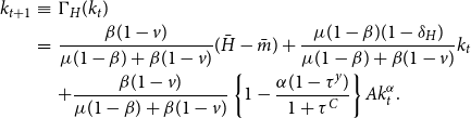(72) \begin{eqnarray} k_{t+1}&\equiv & \Gamma _H(k_t)\nonumber \\ &=&\frac {\beta (1-v)}{\mu (1-\beta)+\beta (1-v)}(\bar {H}-\bar {m}) +\frac {\mu (1-\beta)(1-\delta _H)}{\mu (1-\beta)+\beta (1-v)}k_t \nonumber \\ & & +\frac {\beta (1-v)}{\mu (1-\beta)+\beta (1-v)}\left \{ 1-\frac {\alpha (1-\tau ^y)}{1+\tau ^C} \right \}Ak_t^\alpha. \end{eqnarray}

As previously shown, we define $\hat {k}_H$ such that $\Gamma _{H}^{\prime }(\hat {k}_H)=1$ , given as

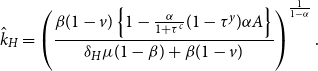(73) \begin{eqnarray} \hat {k}_H=\left (\frac {\beta (1-v)\left \{ 1-\frac {\alpha }{1+\tau ^c}(1-\tau ^y)\alpha A \right \}}{\delta _H \mu (1-\beta)+\beta (1-v)}\right)^{\frac {1}{1-\alpha }}. \end{eqnarray}

We then have the following cases.

When mitigation is provided by the government, its size relative to natural adaptation is key to determining the characteristics of the steady state. As public investment in abatement crowds out capital accumulation, the dynamics of capital shown in (72) shifts downward and modifies the steady states.

Then, are the public mitigation and private adaptation complementary? To answer this question, we first derive how the capital stock is affected by an increase in the mitigation from (72) at the stable steady state.

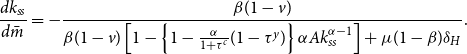(74) \begin{eqnarray} \frac {dk_{ss}}{d\bar {m}}=-\frac {\beta (1-v)}{\beta (1-v)\left [1-\left \{1-\frac {\alpha }{1+\tau ^c}(1-\tau ^y)\right \}\alpha A k_{ss}^{\alpha -1} \right]+\mu (1-\beta)\delta _H}. \end{eqnarray}

The mitigation increases $k_{ss}$ when the capital stock is sufficiently small but decreases $k_{ss}$ when it is large enough. For more detail, we substitute $k_{ss}=\hat {k}_H$ of (73) into (74). Then, the denominator of (74) turns to $0$ . As the capital stock approaches to $\hat {k}_H$ from $0$ , $\frac {dk_{ss}}{d\bar {m}}$ diverges to $+\infty$ . From Proposition8 and Appendix F, the capital stock at the stable steady states is greater than $\hat {k}_H$ . Therefore, at the stable steady states, we always have $\frac {dk_{ss}}{d\bar {m}}\lt 0$ .

Second, we derive a total derivative of $h_{ss}$ and $\bar {m}$ in (71) and obtain the following:

(75) \begin{eqnarray} \frac {dh_{ss}}{d\bar {m}}=\frac {\mu (1-\beta)\left [-1+\left \{(1-\tau ^y)(1-\alpha)+\tau ^y+\frac {\alpha }{1+\tau ^c}(1-\tau ^y)\alpha \right \}\alpha A k_{ss}^{\alpha -1}\frac {dk_{ss}}{d\bar {m}}-(1-\delta _H)\frac {dk_{ss}}{d\bar {m}} \right] }{\mu (1-\beta)+\beta (1-v)}. \notag\\ \end{eqnarray}

From this expression, since the third term in square brackets on the numerator is positive ( $-(1-\delta _H)\frac {dk_{ss}}{d\bar {m}}\gt 0$ ), the adaptation may increase when $k_{ss}$ is large enough. However, we have $\lim _{k_{ss}\rightarrow +\infty }\frac {dk_{ss}}{d\bar {m}}=-\frac {\beta (1-v)}{\beta (1-v)+\mu (1-\beta)\delta _H}$ from (74), and thereby $\lim _{k_{ss}\rightarrow +\infty } \frac {dh_{ss}}{d\bar {m}}=-\frac {\mu (1-\beta)\delta _H}{\beta (1-v)+\mu (1-\beta)\delta _H}\lt 0$ from (75). Discussion so far provides the following proposition.

Whether adaptation and mitigation are complements or substitutes depends not only on the level of the capital stock and the policy instruments (propositions3 and 6), but also on who provides what (Proposition9). Public mitigation directly crowds out private adaptation as a substitution effect. Although savings and thus the capital stock could be increased instead, the steady-state capital stock does not increase from (74). This implies that the government intervention is so large that the income effect from the increased mitigation is negative for private adaptation.