


1. Introduction
The aim of our paper is to examine a general mandate framework for welfare-optimal monetary policy that combines a choice of simple mandates with simple instrument rules that include a trend inflation target. The instrument of monetary policy, the nominal interest rate, faces a zero-lower bound (ZLB) in the form of a low probability of a ZLB incident, a policy choice imposed through a penalty function for the central bank. By comparing outcomes with different probabilities of hitting the ZLB, we also assess the welfare cost of this constraint on monetary policy. The novelty of our study is the integration of these features, which are found separately in the literature, in a complementary and consistent fashion. Our framework ranks different mandates and for each assesses the welfare costs of simplicity and of the ZLB constraint. We follow generally accepted principles in both the academic and central bank communities that monetary policy should be conducted allowing for central bank instrument independence, but goal dependence, based on the principles of commitment, accountability and transparency.Footnote 1 By a credible commitment to future policies, central banks are then able to influence expectations that achieve the best trade-offs from a welfare perspective.
In accordance with these general principles, we study the welfare properties of four different simple mandates each of which consists of four components: (i) a welfare objective delegated to the central bank in the form of a simple transparent quadratic loss function that penalizes deviations from target macroeconomic variables indicating “bliss points” in utility; (ii) a form of a simple Taylor-type nominal interest-rate rule that responds to the same target variables specified in the loss function, thus enhancing transparency; (iii) a ZLB constraint on the nominal interest rate in the form of a specified unconditional probability of ZLB episodes imposed by a further quadratic term penalizing interest rate volatility; and (iv) a long-run (steady-state) inflation target. The weights on the deviations from target variables in the mandate are then chosen to maximize the actual intertemporal utility of the household. Since the form of the mandate is specified for the welfare measure (modified to include the penalty term), the rule and the long-run inflation, these four features make the central bank goal-dependent; but it remains free to choose the strength of its response to the targets in the rule so in that sense it is instrument-independent. We formalize policy in terms of a delegation game with the independent central bank, as the follower, setting the nominal interest rate and a government, as the leader, designing the mandate consisting of components (i) to (iv).
An estimated standard New Keynesian model of Smets and Wouters (Reference Smets and Wouters2007) is used to rank the welfare-optimal mandates with these properties using the expected intertemporal welfare of the household as the ultimate design criterion. Our framework then enables us to assess the welfare costs of simplicity in both mandates and rules, and the cost of the ZLB constraint. The latter is achieved by a combination of a penalty on volatility of the interest rate and an upward shift in the inflation trend.
The Ramsey optimum, used as a benchmark, maximizes the welfare criterion subject only to the constraints of the model and so removes all these costs associated with components (i)–(iv). As well as simple mandates, to quantify the costs of a simple mandate, we study an intermediate regime for which the welfare objective per period in (i) is the household utility again with interest rate volatility penalty. We term this case the ZLB delegation game.
Our paper contributes to two strands of literature: the optimal inflation target given ZLB considerations and optimal mandates. These are reviewed below but here we first highlight two papers that are particularly close to ours. The first is Coibion et al. (Reference Coibion, Gorodnichenko and Wieland2012) (henceforth CGW) who extend the standard linear-quadratic optimal analysis of Woodford, Reference Woodford2003) for a workhorse NK model with no capital, a fully flexible wage (with no stickiness), a zero net trend inflation to the positive trend-inflation case. The model is calibrated to first and second moments of the data. They solve for the duration of a ZLB episode endogenously and examine the trend inflation rate buffer that yields a probability of 5% per quarter of the nominal interest rate hitting the ZLB, the latter calibrated from the data. They show that welfare cost of a positive level of inflation target results in an inflation target close to 2% per year. We extend the model to Smets and Wouters (Reference Smets and Wouters2007) (with some changes explained later) to include capital, sticky-wages and capacity utilization. Our model uses Bayesian estimation and data up to 2017:4 that covers the post-financial-crisis ZLB period using the Mu-Xia shadow rate from 2009:1 onwards.Footnote 2
The second paper is Debortoli et al. (Reference Debortoli, Kim, Linde and Nunes2019) (henceforth DKLN) who develop a mandate framework for which, as in our study, a central bank is instrument-independent and goal-dependent. Our paper differs from this paper in a number of ways. First, we require the central bank to conduct its monetary policy in the form of an optimized simple Taylor-type interest rate rule (OSR) with targets corresponding to those in the welfare goal mandate and with an imposed optimal shift in the trend inflation rate (as in CGW). Second, we formalize the ZLB constraint on the nominal interest rate. Our general approach is to utilize a nonlinear set-up that enables us to employ a second-order perturbation solution of the model with a particular simple interest-rate rule. Then combined with a penalty function we calculate the exact modified social welfare value used by the central bank to compute optimized simple rules. Similarly the design of optimal mandates uses the exact true social welfare without the penalty. In this way, we avoid the quadratic approximation in the linear-quadratic framework of DKLN. Finally, we formalize our framework as a delegation game.
1.1. Main results
Our results can be summarized as follows. We report these highlights in relation to features (i)–(iv) of the mandate framework.
First, in relation to feature (i), in the quadratic mandates, the optimal weights attached to real economic activities (i.e., output or labor demand) are relatively small compared with the weight attached to quarterly price inflation. Only for mandate III targeting directly both nominal price and real wage growth do we find that the relative optimal weights attached to these targets are close to unity. This result contrasts with the strong support for the dual mandate found by DKLN where with a mandate with real activity output growth a weight of almost 3 is reported. The main reason for this difference lies in the trend-inflation effect that is removed in Smets and Wouters (Reference Smets and Wouters2007), but present in our set-up, that makes price and wage dispersion respond up to first order to shocks to price and wage inflation. This creates a reason for policy to react more to changes in the inflation rate and real wage growth for both the instrument rule and the comparable mandate. Another source of the difference is the nature of the delegation game: whereas DKLN studies a Ramsey problem with the simple loss function as parsimonious approximations to social welfare, our paper investigates a simple rule regime where the central bank has delegated a comparable loss function under a presence of the ZLB constraint. These two features limit the ability of the nominal interest rate to respond to any macroeconomic variable and shifts both the rule and the mandates toward the inflation or wage growth targets.
Second, in relation to feature (ii), the associated optimized simple rules all converge to one close to a price-level targeting rule for all mandates with the important exception of the wage-targeting rule. This extreme inertia in the optimized rule arises as a result of the interest rate variability that imposes the ZLB constraint. This result supports a large recent literature highlighting the benefits of “make-up strategies” of which price-level targeting is a special case (see the next subsection for further discussion).
Finally, in relation to (iii) and (iv), using the calibrated quarterly probability of $\bar{p}_{zlb} =0.05$
or 5% (approx 5 quarters every 25 years) as in CGW which they note is consistent with the historical experience of the ZLB frequency for the USA from 1945 to 2012, we find the optimal trend inflation is 2.4% so is close to the typical annual 2% of most prominent central banks. In our sample from 1958 to 2017 that includes a long ZLB period, we find that the corresponding frequency is higher at
$\bar{p}_{zlb} =0.05$
or 5% (approx 5 quarters every 25 years) as in CGW which they note is consistent with the historical experience of the ZLB frequency for the USA from 1945 to 2012, we find the optimal trend inflation is 2.4% so is close to the typical annual 2% of most prominent central banks. In our sample from 1958 to 2017 that includes a long ZLB period, we find that the corresponding frequency is higher at $\bar{p}_{zlb} = 0.096$
, which leads to a lower optimal inflation trend of 1.6%. On the other hand, to support a tighter ZLB constraint of
$\bar{p}_{zlb} = 0.096$
, which leads to a lower optimal inflation trend of 1.6%. On the other hand, to support a tighter ZLB constraint of $\bar{p}_{zlb}=0.01$
, we require an inflation trend close to 4% as has been proposed in the literature (see Section 6.4 for further discussion).
$\bar{p}_{zlb}=0.01$
, we require an inflation trend close to 4% as has been proposed in the literature (see Section 6.4 for further discussion).
1.2. Related literature
In addition to the two highlighted papers above, our paper is also related to the literature on simple objectives, simple rules, price-level as opposed to inflation targeting, the optimal long-run (steady state) inflation target and (in relation to DKLN) approximating optimal policy as a tractable linear-quadratic problem. We consider these in turn.
Simple Objectives. In what has been an influential paper with central banks, Rudebusch and Svensson (Reference Rudebusch, Svensson, Rudebusch and Svensson1999) examine two broad classes of rules referred to as “instrument’ and ‘targeting rules.” The former are our simple nominal interest-rate rules. Their “targeting rule” is an assignment of a welfare loss function over deviations of goal variables from their targets (in effect bliss points) corresponds to the loss function in our mandate. In our paper, quadratic loss functions are seen as transparent simple mandates and not the best approximation of the household utility. But as is well-known, in the simple work-horse three-equation NK model with price stickiness Woodford, Reference Woodford2003), Chapter 6, shows that a quadratic function in inflation and the output gap is an accurate approximation up to second order. However this no longer applies to the Smets and Wouters (Reference Smets and Wouters2007) model we employ with capital, wage stickiness, and variable capacity utilization.
Simple Rules. There is an old macroeconomics literature on the assignment of instruments and targets using simple rules going back to Mundell (Reference Mundell1962) and developed by Vines et al. (Reference Vines, Maciejowski and Meade1983), and Weale et al. (Reference Weale, Blake, Christodoulakis, Meade and Vines1989). In particular, the case for simplicity in the choice of nominal interest rate rules is associated with Taylor (Reference Taylor1993, Reference Taylor and Taylor1999) and is re-iterated in Woodford (Reference Woodford2003), Chapter 7, Section 3. Such rules that are welfare optimal within a particular class of simplicity are studied in Schmitt-Grohe and Uribe (Reference Schmitt-Grohe and Uribe2007) for both monetary and fiscal policy using perturbation methods (see also Kim et al. (Reference Kim, Kim, Schaumburg and Sims2003) for the latter). An alternative to an optimized simple rule is the fully optimal Ramsey problem that maximizes the expected household intertemporal utility leads to a complicated history-dependent rule (see Levine and Currie (Reference Levine and Currie1987)) that would be difficult for the government to implement and monitor. The latter implies that commitment would be difficult. By contrast simple Taylor-type rules are easy to implement and monitor. Schmitt-Grohe and Uribe (Reference Schmitt-Grohe and Uribe2007) show that the optimal form of the latter, welfare-optimized simple rules, can closely mimic the former. This is now broadly accepted in the literature and we find it to be true on our paper. As we show later in Section 5.3 as with the Ramsey solution, such rules are still time inconsistent, but their simplicity implies any deviation from the rule would be punished by a loss of credibility. Another advantage of simple rules is that they have good robustness properties in the face of model uncertainty (see Levine et al. (Reference Levine, McAdam and Pearlman2012) and Deak et al. (Reference Deak, Levine, Mirza and Pearlman2021b)).
Price-Level Targeting. Finally, our paper adds to a strand of literature that highlights the benefits of price-level targeting (see, for example, Svensson (Reference Svensson1999), Schmitt-Grohe and Uribe (Reference Schmitt-Grohe and Uribe2000), Vestin (Reference Vestin2006), Reiss (Reference Reiss2009), Gaspar et al. (Reference Gaspar, Smets, Vestin, Gaspar, Smets and Vestin2010), Giannoni (Reference Giannoni2014)). These papers examine the good determinacy and stability properties of price-level targeting. Holden (Reference Holden2016) shows these benefits extend to a ZLB setting. A very recent literature describes these benefits in terms of “make-up” strategies for central banks and in particular the Federal Reserve; see Powell (Reference Powell2020), Svensson (Reference Svensson2020). Under such strategies, the central banks seek to redress past deviations of inflation from its target. Assuming a make-up rule enjoys credibility, undershooting (overshooting) the target will raise (lower) inflation expectations, lower (raise) the real interest rate, and help to stabilize the economy. Inertial Taylor rules have by design the make-up feature as they commitment to a response of the nominal interest rate to a weighted average of past inflation with the weights increasing with the degree of inertia. “Average inflation targeting” is a variant that sets a rolling window of cumulative past deviations; a further variant sets an asymmetric target whereby the central bank responds to average inflation above and below the long-run target in a different way. Hebden et al. (Reference Hebden, Herbst, Tang, Topa and Winkler2020) provide details of these different makeup strategies and analyze their effectiveness using the Federal Reserve US macroeconomic model. Giannoni and Woodford (Reference Giannoni and Woodford2003) and Giannoni (Reference Giannoni2014) study the Ramsey problem with an interest rate penalty function and show that the optimal policy can be implemented as a second-order interest rate rule with “super-inertia” as explained in Subsection 5.2. In our paper, we study optimized inertial (but not super-inertial) Taylor rules that are parameterized so as to encompass a simple form of price-level targeting—see Section 5.
The Optimal Inflation Target. A number of papers simulate large-scale models in which a central bank commits to a version of the Taylor rule to explore the optimal level of target inflation. Reifschneider and Williams (Reference Reifschneider and Williams1999) and Günter et al. (Reference Günter, Athanasios and Volker2004) find a 2% inflation target to be an adequate buffer against the ZLB having noticeable adverse effects on the economy. However, these authors do not consider the costs associated with a higher average inflation rate. A more recent strand of literature studies the optimal level of inflation target under the ZLB and incorporates such costs; for example, Ascari and Ropele (Reference Ascari and Ropele2007), CGW (discussed above), Dordal-i-Carreras et al. (Reference Dordal-i-Carreras, Coibion, Gorodnichenko and Wieland2016), Ngo (Reference Ngo2018) and Andrade et al. (Reference Andrade, Galí, Le Bihan and Matheron2019). But other papers argue that the 2% inflation target is too low and a target inflation of 4% would be adequate and would not harm an economy significantly (see Ball (Reference Ball2013)). However, Ascari and Sbordone (Reference Ascari and Sbordone2014) and Kara and Yates (Reference Kara and Yates2017) argue that with a higher level of inflation target the determinacy region is significantly reduced. The latter paper in particular finds in a model of heterogeneity in price stickiness when trend inflation is 4% that the determinacy region in the model is almost nonexistent. This result is particularly relevant for our results. In our mandates, the central bank chooses an optimized form of the monetary rule which is constrained by the need for determinacy; by choosing an interest-rate rule with considerable persistence (in fact close to a price-level rule), the indeterminacy problem is avoidedFootnote 3 and a 4% target with its associated low probability of ZLB episodes becomes possible.
Linear Quadratic Framework. The approach of DKLN approximates a nonlinear optimization problem for the central bank with linear-quadratic (LQ) problem closely following Benigno and Woodford (Reference Benigno, Woodford, Benigno and Woodford2004) and Levine et al. (Reference Levine, Pearlman and Pierse2008a). The quadratic form of the utility is no longer necessarily simple. The LQ approach omits second-order dynamics of the model captured in our perturbation solution. However, it does have the advantage (not exploited in DKLN) that it facilitates, even for large models, the computation of a discretionary equilibrium at the CB monetary rule decision stage of the delegation game. Details of this approach are provided in Appendix (E).
1.3. Road-map
The rest of the paper’s structure is organized as follows: in the next section, we briefly represent a simple analysis of trend inflation, probability of hitting the ZLB, penalty function on the ZLB, and the delegation game. We then present the full Smets–Wouter New Keynesian model (Smets and Wouters (Reference Smets and Wouters2007)) which is estimated by Bayesian methods with different data series of the nominal interest rate, namely the standard Federal funds rate and the shadow interest rate (Wu & Xia, Reference Wu and Xia2016)). We then introduce the general monetary policy delegation game between different agents in the economy which leads to the main numerical results of the paper. Concluding comments complete the paper.
2. Key features of the analysis
In order to understand the key mechanisms at play for monetary policy, we now elaborate on the key features of our analysis.
2.1 The optimal trend inflation: Welfare effects and the ZLB
A crucial feature of an welfare-optimized monetary policy rule is the optimal level of inflation target (the chosen inflation trend) in the optimized rule. In our sticky-price and sticky-wage model, a positive trend inflation is costly to the economy through both a steady-state effect and dynamic effects. The former is the more important, so we examine this in some detail. For simplicity, consider the zero growth case $g=0$
for which wage and price inflation are equal. Then for price-setting the impact of trend inflation
$g=0$
for which wage and price inflation are equal. Then for price-setting the impact of trend inflation $\Pi$
on the deterministic steady state is given by
$\Pi$
on the deterministic steady state is given by
 \begin{align*} \frac{P^{0}}{P} &= \left(\frac{1-\xi _p \Pi ^{(1-\gamma _p)(\zeta _p-1)}}{1-\xi _p}\right)^{\frac{1}{1-\zeta _p}} \\ \Delta _{p} &= \frac{1-\xi _p}{1-\xi _p\Pi ^{\zeta _p(1-\gamma _p)}} \left(\frac{P^0}{P}\right)^{-\zeta _p} \\ MC &= \left(1-\frac{1}{\zeta _p}\right) \frac{1-\xi _p \beta \Pi ^{\zeta _p(1-\gamma _p)}}{1-\xi _p \beta \Pi ^{(\zeta _p-1)(1-\gamma _p)}}\frac{P^{0}}{P} \end{align*}
where $\frac{P^{0}}{P}$
is the reoptimized Calvo-price for each retail variety, reset with probability
$\frac{P^{0}}{P}$
is the reoptimized Calvo-price for each retail variety, reset with probability $\xi _p$
,
$\xi _p$
, $\zeta _p$
is the price-elasticity of demand
$\zeta _p$
is the price-elasticity of demand $\Delta _{p}$
is price dispersion across varieties,
$\Delta _{p}$
is price dispersion across varieties, $MC$
is the real marginal cost equal to the inverse of the price mark-up,
$MC$
is the real marginal cost equal to the inverse of the price mark-up, $\gamma _p \in [0,1]$
is the degree of price-indexing and
$\gamma _p \in [0,1]$
is the degree of price-indexing and $\beta$
is the household discount factor.Footnote
4
$\beta$
is the household discount factor.Footnote
4
For wage-setting, we have analogous results:
 \begin{align*} \frac{W_n^{O}}{W_n} &= \left(\frac{1-\xi _w \Pi ^{(1-\gamma _w)(\zeta _w-1)}}{1-\xi _w}\right)^{\frac{1}{1-\zeta _w}}\\ \Delta _{w} &= \frac{1-\xi _w}{1-\xi _w \Pi ^{(1-\gamma _w)\zeta _w}} \left(\frac{W_n^O}{W_n}\right)^{-\zeta _w}\\ \frac{W_{h}}{W} & =\frac{\left(1-\xi _w \beta \Pi ^{(1-\gamma _w)\zeta _w}\right)\left(1-\frac{1}{\zeta _w}\right)\frac{W_n^{O}}{W_n} }{1-\xi _w \beta \Pi ^{(1-\gamma _w)(\zeta _w-1)}}. \end{align*}
where $\frac{W_n^{O}}{W_n}$
is the reoptimized Calvo nominal wage for each labor variety, reset with probability
$\frac{W_n^{O}}{W_n}$
is the reoptimized Calvo nominal wage for each labor variety, reset with probability $\xi _w$
,
$\xi _w$
, $\zeta _w$
is the wage elasticity of demand
$\zeta _w$
is the wage elasticity of demand $\Delta _{w}$
is nominal wage dispersion across varieties,
$\Delta _{w}$
is nominal wage dispersion across varieties, $\gamma _w \in [0,1]$
is the degree of nominal wage indexing and
$\gamma _w \in [0,1]$
is the degree of nominal wage indexing and $\frac{W_{h}}{W}$
is the inverse of the real wage mark-up over the real wage homogeneous labor rate
$\frac{W_{h}}{W}$
is the inverse of the real wage mark-up over the real wage homogeneous labor rate $W_{h}$
at which households supply hours.
$W_{h}$
at which households supply hours.
Thus for $\zeta _p\gt 1$
, both the optimized price
$\zeta _p\gt 1$
, both the optimized price $\frac{P^{0}}{P}$
and price dispersion
$\frac{P^{0}}{P}$
and price dispersion $\Delta _{p}$
increase with the trend inflation rate
$\Delta _{p}$
increase with the trend inflation rate $\Pi$
. However, noting that the price mark-up is the inverse of the real marginal cost, that is, equal to
$\Pi$
. However, noting that the price mark-up is the inverse of the real marginal cost, that is, equal to $=1/MC$
, we can see that the price response to the reoptimized price decreases with
$=1/MC$
, we can see that the price response to the reoptimized price decreases with $\Pi$
. Analogous results for
$\Pi$
. Analogous results for $\zeta _w\gt 1$
hold for the optimized nominal wage, wage dispersion, and the wage mark-up which is the inverse of
$\zeta _w\gt 1$
hold for the optimized nominal wage, wage dispersion, and the wage mark-up which is the inverse of $\frac{W_{h}}{W_n}$
. Taking these results together, we then have two effects of trend inflation that increase distortions from sticky prices and wages and thus reduce welfare whereas the third effect results in the opposite. However, numerical results based on our estimated model confirms that the former easily outweighs the latter.Footnote
5
$\frac{W_{h}}{W_n}$
. Taking these results together, we then have two effects of trend inflation that increase distortions from sticky prices and wages and thus reduce welfare whereas the third effect results in the opposite. However, numerical results based on our estimated model confirms that the former easily outweighs the latter.Footnote
5
We now turn to the dynamic effect of trend inflation which was first studied by Ascari and Ropele (Reference Ascari and Ropele2007). They show it leads to richer inflation dynamics and a higher inflation volatility. They also show that the Taylor principle is no longer sufficient to guarantee a unique rational expectations equilibrium in New Keynesian models for even moderate levels of inflation. CGW argue that a greater steady-state inflation induces a higher level of its forward-looking dynamic behavior when sticky-price firms are able to reset their prices. The more forward-looking is a firm, the greater is then anticipation of other firms raising the optimal reset price. These dynamic considerations point to further welfare costs of high trend inflation. Fig. 1 previews the dynamic effects of trend inflation for the stochastic steady state of our estimated model, set out in the rest of the paper, with the CB choosing an optimized general interest rate rule that maximizes expected household intertemporal welfare (without, as yet, ZLB considerations).
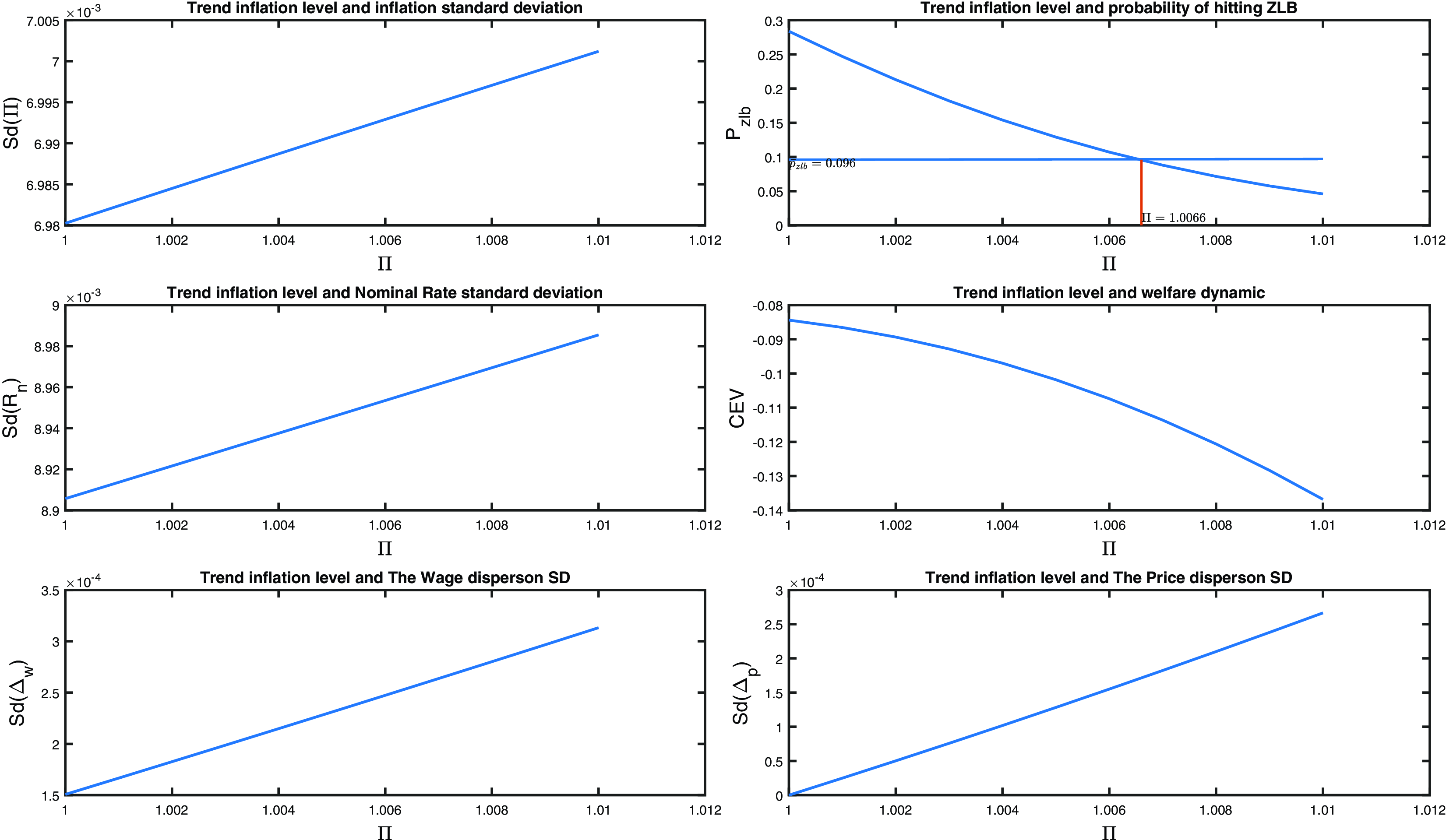
Figure 1. The effects of trend inflation, $\Pi$
, in the stochastic steady state. The consumption equivalent variations (CEV) is the welfare gain(loss) with different monetary regimes, expressing with different values of steady-state inflation, the representative household’s welfare compared to when the central bank pursues a monetary policy regime at the Ramsey. The figure is produced by stimulating the estimated Smets and Wouters (Reference Smets and Wouters2007) model (presented below) for different values of trend inflation.
$\Pi$
, in the stochastic steady state. The consumption equivalent variations (CEV) is the welfare gain(loss) with different monetary regimes, expressing with different values of steady-state inflation, the representative household’s welfare compared to when the central bank pursues a monetary policy regime at the Ramsey. The figure is produced by stimulating the estimated Smets and Wouters (Reference Smets and Wouters2007) model (presented below) for different values of trend inflation.
We see the positive relationship between the level and volatility of inflation, a well-documented result in the empirical literature, associated with an increasing volatility of the nominal interest rate, $R_{n,t}$
. Thus, the distribution of
$R_{n,t}$
. Thus, the distribution of $R_{n,t}$
as well as shifting to the right becomes wider. The net effect on the probability of hitting the ZLB can therefore be positive or negative, but given the estimation and optimized rule the first effect dominates and the probability falls.
$R_{n,t}$
as well as shifting to the right becomes wider. The net effect on the probability of hitting the ZLB can therefore be positive or negative, but given the estimation and optimized rule the first effect dominates and the probability falls.
A positive trend inflation then increases distortions caused by sticky prices and wages by increasing both the steady state and the volatility of both price and wage dispersion (see Fig. 1 for the latter) and is welfare-reducing. But on the other hand, a positive inflation trend reduces the frequency of the nominal interest rate hitting the ZLB constraint. Frequent ZLB incidents are an undesirable feature of a monetary rules because, as Christiano et al. (Reference Christiano, Eichenbaum and Rebelo2011) argue, a zero-bound scenario involves a deflationary spiral which contributes to and accompanies a large fall in output, which leads to a high volatility and large output cost. Specifically, when output falls, marginal cost falls and price declines. With staggered pricing, a drop in price causes agents to expect a deflation in the future. With the nominal interest rate stuck at zero, the real interest rate rises, which leads to an increase in desired saving and a decrease in output. As a result, the cumulative fall in output required to reduce desired saving to zero is extremely significant. These considerations lead us to design a monetary rule with a low probability of ZLB episodes.
Are there then welfare benefits from increasing trend inflation given the desirability of avoiding such adverse zero-bound episodes? Should then the optimal level of inflation target set by the central bank be close to the typical target inflation of 2% or is the inflation target too blunt an instrument to efficiently reduce the severe costs of zero-bound episodes. This is one of the research questions we now pursue in our general mandate framework.
2.2 The ZLB constraint through a penalty function
In this paper, we adopt a penalty function approach to the imposition of a ZLB constraint on the nominal net interest rate. It is distinguished from the imposition of a ZLB occasionally binding constraint. For the latter standard perturbation methods are unavailable as the policy function is nondifferentiable at the constraint, but the option of a global solution by value function iteration methods is possible (see, for example, Guerrieri and Iacoviello (Reference Guerrieri and Iacoviello2015)). However, this option suffers from the curse of dimensionality unless the state space is small. This problem becomes acute when the model solution is embedded in our mandate framework that involves the computation of optimized rules. Our solution then is to use an approximate perturbation-based method with a penalty function that imposes the constraint in a continuously binding form.
There are two common approaches to this method: first, to add the penalty term to the policy-maker’s welfare criterion (see Woodford, Reference Woodford2003), Giannoni and Woodford (Reference Giannoni and Woodford2003), Levine et al. (Reference Levine, McAdam and Pearlman2008b, Reference Levine, McAdam and Pearlman2012), Giannoni (Reference Giannoni2014)); second, to add the penalty term to the agents’ welfare criteria in the model (see Den Haan and Wind (Reference Den Haan and Wind2012), Abo-Zaid (Reference Abo-Zaid2015), Karmakar (Reference Karmakar2016)). The general idea is that instead of truncating the state space of the model at the constraint, we introduce a welfare penalty if the constraint is violated; this penalty acts as a constraint while maintaining differentiability of the policy functions. More precisely, we allow the nominal interest rate hit the zero bound with a small probability which can be interpreted as the tightness level of the ZLB constraint.Footnote 6 Our paper follows this literature by adding a penalty term on the central bank’s objective function. We also compare different mandate formations delegated to the central bank, namely: a so-called ZLB mandate which retains the household utility as a welfare measure, a number of simple quadratic loss function mandates, and an asymmetric functional form mandate.
2.3 The delegation game
We now turn to simple quadratic loss function mandates designed to increase transparency in the conduct of monetary policy. In the simple mandates we choose the particular loss function is matched with a simple rule with the same targets. Thus, the transparency of the loss function is reinforced with that of the interest rate rule. Our mandates are expressed in terms of the growth of a real variable $X_t$
,
$X_t$
, $\frac{X_t}{X_{t-1}}$
and gross inflation
$\frac{X_t}{X_{t-1}}$
and gross inflation $\Pi _t$
relative to their steady states. In the simple mandates, we study the real variable can be output, the real market-clearing wage paid by the firm and hours employed. The mandate delegated to the central bank then consists of a welfare criterion:
$\Pi _t$
relative to their steady states. In the simple mandates, we study the real variable can be output, the real market-clearing wage paid by the firm and hours employed. The mandate delegated to the central bank then consists of a welfare criterion:
 \begin{eqnarray} \Omega _t^{mod} \equiv - \mathbb{E}_t\left [ \sum _{\tau =0}^\infty \beta ^{\tau } \left(\left(\Pi _{t+\tau } - \Pi \right)^2 + w_{dx} \left(\frac{X_{t+\tau }}{X_{t+\tau -1}} - (1+g) \right)^2 + w_r \left(R_{n,t+\tau } - R_n \right)^2 \right) \right ] \end{eqnarray}
with a corresponding simple rule for the nominal gross interest rate $R_{n,t}$
, the monetary instrument given by
$R_{n,t}$
, the monetary instrument given by
 \begin{equation} \log \left( \frac{R_{n,t}}{R_n}\right)=\rho _r \log \left( \frac{R_{n,t-1}}{R_n}\right) +\alpha _\pi \log \left(\frac{\Pi _{t}}{\Pi }\right) + \alpha _{dx} \log \left(\frac{X_t}{X_{t-1}}\right) \end{equation}
A two-stage quadratic loss function delegation game then defines an equilibrium in choice variables by the leader (the policymaker) $w_{dx}^*$
,
$w_{dx}^*$
, $w_r^*$
, and
$w_r^*$
, and $\Pi ^*$
and a choice
$\Pi ^*$
and a choice $\rho ^* \equiv [ \rho _r^*, \alpha _\pi ^*, \alpha _{dx}^*]$
by an independent central bank (the follower) that maximizes the actual household welfare subject to the ZLB constraint that maximizes the actual household intertemporal welfare given by
$\rho ^* \equiv [ \rho _r^*, \alpha _\pi ^*, \alpha _{dx}^*]$
by an independent central bank (the follower) that maximizes the actual household welfare subject to the ZLB constraint that maximizes the actual household intertemporal welfare given by
 \begin{eqnarray} \Omega _t=\mathbb{E}_t\left [ \sum _{\tau =0}^\infty \beta ^{\tau } U_{t+\tau }\right ] \end{eqnarray}
where $U_t$
is the single-period utility of the representative household. The central bank is instrument independent in the sense that it is free to choose
$U_t$
is the single-period utility of the representative household. The central bank is instrument independent in the sense that it is free to choose $\rho ^*$
given the mandate that specifies its objective (1) and form of rule (2).
$\rho ^*$
given the mandate that specifies its objective (1) and form of rule (2).
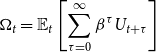
In an intermediate regime we first examine a ZLB delegation game with a modified welfare measure delegated to the central bank based on (3) with a penalty term designed to limit the variance of the nominal interest rate:
 \begin{eqnarray} \Omega _t^{mod} &\equiv & \mathbb{E}_t\left [ \sum _{\tau =0}^\infty \beta ^{\tau } \left(U_{t+\tau } - w_r \left(R_{n,t+\tau } - R_n \right)^2 \right)\right ] \end{eqnarray}
and a simple Taylor-type rule of the same form as that estimated in Section 4.
 \begin{equation} \log \left( \frac{R_{n,t}}{R_n}\right)=\rho _r \log \left( \frac{R_{n,t-1}}{R_n}\right) +\alpha _\pi \log \left(\frac{\Pi _{t}}{\Pi }\right) + \alpha _y \log \left(\frac{Y_t}{Y}\right) + \alpha _{dy} \log \left(\frac{Y_t}{Y_{t-1}}\right) \end{equation}
Our welfare criteria $\Omega _t^{mod}$
and
$\Omega _t^{mod}$
and $\Omega _t$
are conditional, evaluated at the deterministic zero net inflation steady state and responding to all future shocks. We distinguish two welfare criteria in this delegation game: first, the modified welfare,
$\Omega _t$
are conditional, evaluated at the deterministic zero net inflation steady state and responding to all future shocks. We distinguish two welfare criteria in this delegation game: first, the modified welfare, $\Omega _t^{mod}$
, is the welfare criterion of the central bank. Second, the actual welfare,
$\Omega _t^{mod}$
, is the welfare criterion of the central bank. Second, the actual welfare, $\Omega _t$
, is the welfare criterion of the representative household. Full details of these two delegation games are given in Sections 5 and 6.
$\Omega _t$
, is the welfare criterion of the representative household. Full details of these two delegation games are given in Sections 5 and 6.
Two research question regarding the mandates are then first, what is the cost of simplicity in adopting quadratic mandate compared with the benchmark as the ZLB constraint becomes tighter and second, what are the relative weights attached to real economic activities compared with the (unit) weight attached to price inflation.
3. A non-linear medium-sized NK model with trend inflation
Most papers using the Smets and Wouters (Reference Smets and Wouters2007) model use the linearized form about a balanced-nonzero growth and effectively zero-net-inflation steady state.Footnote 7 The nonlinear form of the model with a trend net inflation is relatively unexplored, but is essental for the welfare analysis of this paper which is based on a second-order perturbation solution. The properties of the model in a nonzero-net inflation rate steady state, set out in Section 2.1), are crucial in this set-up. This section therefore sets the full non-linear form to be solved in the vicinity of a trend net inflation deterministic steady state.
There are four sets of representative agents: households, final goods producers, trade unions, and intermediate goods producers. The later two produce differentiated labor services and goods, respectively, and, in each period of time, consist of a group that is locked into an existing contract and another group that can reoptimize.Footnote 8
3.1 Households
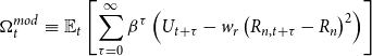
At time $t=0$
, household
$t=0$
, household $i$
maximizes its expected lifetime utility
$i$
maximizes its expected lifetime utility
 \begin{eqnarray} \Omega _0(i)&=&\mathbb{E}_0 \sum _{t=0}^\infty \beta ^t U_t(C_t(i), C_{t-1}(i), H_t^s(i)\nonumber \\&=&\mathbb{E}_0 \left [\sum _{t=0}^\infty \beta ^t \frac{\left [C_t(i)-\chi C_{t-1}(i)\right ]^{1-\sigma }}{1-\sigma }\exp \left [(\sigma -1)\frac{ H_t^s(i)^{1+\psi }}{1+\psi }\right ]\right ] \end{eqnarray}
where $\mathbb{E}_t[\cdot ]$
denotes rational expectations based on information available at time
$\mathbb{E}_t[\cdot ]$
denotes rational expectations based on information available at time $t$
,
$t$
, $C_t(i)$
is real consumption,
$C_t(i)$
is real consumption, $H_t^s(i)$
is hours supplied,
$H_t^s(i)$
is hours supplied, $\beta$
is the discount factor,
$\beta$
is the discount factor, $\chi$
controls for internal habit formation,
$\chi$
controls for internal habit formation, $\sigma$
is the inverse of the elasticity of intertemporal substitution (for constant labor), and
$\sigma$
is the inverse of the elasticity of intertemporal substitution (for constant labor), and $\psi$
is the inverse of the Frisch labor supply elasticity. Preferences chosen by SW in (6) are compatible with balanced growth (see King et al. (Reference King, Plosser and Rebelo1988)).
$\psi$
is the inverse of the Frisch labor supply elasticity. Preferences chosen by SW in (6) are compatible with balanced growth (see King et al. (Reference King, Plosser and Rebelo1988)).
The household’s budget constraint in period $t$
is given by
$t$
is given by
 \begin{equation} C_t(i) + I_t(i) + \frac{B_{t}(i)}{RPS_t R_{n,t} P_t} + T_t = \frac{B_{t-1}(i)}{P_t}+ \left(r_t^K u_t(i) - a(u_{t}(i))\right)K_{t-1}(i) + W_{h,t} H_t^s(i)+\Gamma _t \end{equation}
where $I_t$
is investment into physical capital,
$I_t$
is investment into physical capital, $B_t$
is government bonds held at the end of period
$B_t$
is government bonds held at the end of period $t$
,
$t$
, $R_{n,t-1}$
is the nominal interest rate paid on government bonds held at the beginning of period
$R_{n,t-1}$
is the nominal interest rate paid on government bonds held at the beginning of period $t$
,
$t$
, $RPS_t$
is an exogenous premium in the return on bonds that follows an AR1 process.
$RPS_t$
is an exogenous premium in the return on bonds that follows an AR1 process. $T_t$
is lump-sum taxes,
$T_t$
is lump-sum taxes, $r_t^K$
is the real rental rate,
$r_t^K$
is the real rental rate, $u_t$
is the utilization rate of capital,
$u_t$
is the utilization rate of capital, $\mbox{IS}_t$
is an investment specific technological shock (the inverse of the relative price of new capital in consumption terms),
$\mbox{IS}_t$
is an investment specific technological shock (the inverse of the relative price of new capital in consumption terms), $a(u_t(i))$
is the physical cost of use of capital in consumption terms,
$a(u_t(i))$
is the physical cost of use of capital in consumption terms, $W_{h,t}$
is the real wage rate at which households supply labor that is homogeneous at this point to trade unions and
$W_{h,t}$
is the real wage rate at which households supply labor that is homogeneous at this point to trade unions and $\Gamma _t$
is the profit of intermediate firms distributed to households.
$\Gamma _t$
is the profit of intermediate firms distributed to households.
End of period capital stock, $K_t(i)$
, accumulates according to
$K_t(i)$
, accumulates according to
 \begin{align} K_{t}(i)&= (1-\delta ) K_{t-1}(i)+(1-S(X_t(i)))I_t(i) \mbox{IS}_t \end{align}
where $\mbox{IS}_t$
is an investment specific technological shock that follows an AR1 process,
$\mbox{IS}_t$
is an investment specific technological shock that follows an AR1 process, $X_t(i) = I_t(i)/I_{t-1}(i)$
is the growth rate of investment, and
$X_t(i) = I_t(i)/I_{t-1}(i)$
is the growth rate of investment, and $S(\cdot )$
is an adjustment cost function such that
$S(\cdot )$
is an adjustment cost function such that $S(X)=0$
,
$S(X)=0$
, $S'(X)=0$
, and
$S'(X)=0$
, and $S''(\cdot )=0$
where
$S''(\cdot )=0$
where $X$
is the steady-state value of investment growth. For
$X$
is the steady-state value of investment growth. For $S(X_t)$
in a symmetric equilibrium, we choose the functional form:
$S(X_t)$
in a symmetric equilibrium, we choose the functional form: $S(X_t)=\phi _X (X_t-\bar{X}_t)^2$
where
$S(X_t)=\phi _X (X_t-\bar{X}_t)^2$
where $\bar{X}_t$
is the balanced-growth steady-state trend. For
$\bar{X}_t$
is the balanced-growth steady-state trend. For $a(u_t)$
we choose the functional form:
$a(u_t)$
we choose the functional form: $a(u_t)=\gamma _1(u_t-1)+\frac{\gamma _2}{2}(u_t-1)^2$
with
$a(u_t)=\gamma _1(u_t-1)+\frac{\gamma _2}{2}(u_t-1)^2$
with $u_t=u=1$
in the steady state.
$u_t=u=1$
in the steady state.
Then the household first-order conditions consist of an Euler Consumption equation, an arbitrage condition, a first-order condition equating the marginal rate of substitution between leisure and consumption with the real wage and first-order conditions for investment, the price of capital $Q_t$
(Tobin’s Q) and capacity utilization:
$Q_t$
(Tobin’s Q) and capacity utilization:
 \begin{align} \mathbb{E}_t[\Lambda _{t,t+1}(i) R_{t+1}]&=1 \end{align}
 \begin{align} \mathbb{E}_t[\Lambda _{t,t+1}(i) R_{t+1}^K]& =1 \end{align}
 \begin{align} -\frac{U_{H,t}(i)}{U_{C,t}(i)} & =W_{h,t} \end{align}
 \begin{align} Q_t & = \mathbb{E}_t \left \{\Lambda _{t,t+1}(i) \left [r_{t+1}^K u_{t+1}(i) - a(u_{t+1})(i) + Q_{t+1} (1-\delta )\right ]\right \} \end{align}
 \begin{align} 1 &= Q_t\left [1-S(X_t(i))-S'(X_t)(i)X_t(i)\right ]IS_t\nonumber \\ &\quad + \mathbb{E}_{t} \left [\Lambda _{t,t+1} Q_{t+1} S'(X_{t+1}(i))X_{t+1}(i)^2 IS_{t+1} \right ] \end{align}
 \begin{align} r_t^K & =a'(u_t(i)) \end{align}
where $\Lambda _{t,t+1}(i)\equiv \beta \frac{U_{C,t+1}(i)}{U_{C,t}(i)}$
is the stochastic discount factor,
$\Lambda _{t,t+1}(i)\equiv \beta \frac{U_{C,t+1}(i)}{U_{C,t}(i)}$
is the stochastic discount factor, $U_{C,t}(i) \equiv \frac{\partial U_t(i) }{\partial C_t(i)}$
,
$U_{C,t}(i) \equiv \frac{\partial U_t(i) }{\partial C_t(i)}$
, $U_{H,t} (i) \equiv \frac{\partial U_t(i) }{\partial H_t(i)}$
are marginal utilities over two successive periods in the summation given by
$U_{H,t} (i) \equiv \frac{\partial U_t(i) }{\partial H_t(i)}$
are marginal utilities over two successive periods in the summation given by
 \begin{equation} U_{C,t} (i) = (1-\sigma ) \left( \frac{U_t(i)}{C_t(i)-\chi C_{t-1}(i)} -\frac{\beta \chi U_{t+1}(i)}{C_{t+1}(i)-\chi C_{t}(i)} \right) \end{equation} $R_t = \frac{R_{n,t-1}}{\Pi _t}$
and
$R_t = \frac{R_{n,t-1}}{\Pi _t}$
and $R_{t}^K=\frac{[r_t^K u_t-a(u_t)+(1-\delta )Q_{t}]}{Q_{t-1}}$
are the real gross returns on government bonds and physical capital, respectively, and
$R_{t}^K=\frac{[r_t^K u_t-a(u_t)+(1-\delta )Q_{t}]}{Q_{t-1}}$
are the real gross returns on government bonds and physical capital, respectively, and $Q_t$
is the price of capital (Tobin’s Q). In a symmetric equilibrium of identical households
$Q_t$
is the price of capital (Tobin’s Q). In a symmetric equilibrium of identical households $C_t(i)=C_t$
,
$C_t(i)=C_t$
, $H_t^s (i) =H_t^s$
, etc.
$H_t^s (i) =H_t^s$
, etc.
3.2 The labor market
Households supply their homogeneous labor to trade unions that differentiate the labor services. A labor packer buys the differentiated labor from the trade unions and aggregate them into a composite labor using the Dixit–Stigliz aggregatorFootnote
9
given aggregate demand $H_t^d$
.
$H_t^d$
.
 \begin{equation} H_{t}^d=\left( \int _{0}^{1}H_{t}(j)^{(\zeta _w -1)/\zeta _w }dj\right)^{\zeta _w/(\zeta _w -1)} dj \end{equation}
where $\zeta _w$
is the elasticity of substitution among different types of labor, and we index trade unions by
$\zeta _w$
is the elasticity of substitution among different types of labor, and we index trade unions by $j$
. The labor packer minimizes the cost
$j$
. The labor packer minimizes the cost $\int _0^1 W_{n,t}(j) H_t(j) dj$
of producing the composite labor service, where
$\int _0^1 W_{n,t}(j) H_t(j) dj$
of producing the composite labor service, where $W_{n,t}(j)$
denotes the nominal wage set by union
$W_{n,t}(j)$
denotes the nominal wage set by union $j$
. This leads to the standard demand function
$j$
. This leads to the standard demand function
 \begin{align} H_{t}(j)&=\left(\frac{W_{n,t}(j)}{W_{n,t}}\right) ^{-\zeta _w }H_{t}^d \end{align}
where $W_{n,t}$
is the aggregate nominal wage given by the Dixit–Stigliz aggregator
$W_{n,t}$
is the aggregate nominal wage given by the Dixit–Stigliz aggregator
 \begin{equation*} W_{n,t}=\left [ \int _0^1 W_{n,t}(j)^{1-\zeta _w} dj \right ]^{ \frac {1}{1-\zeta _w}} \end{equation*}
Sticky wages are introduced through Calvo contracts supplemented with indexation. At each period there is a probability $1-\xi _{w}$
that trade union
$1-\xi _{w}$
that trade union $j$
can choose
$j$
can choose $W_{n,t}^O(j)$
to maximize
$W_{n,t}^O(j)$
to maximize
 \begin{equation*} \mathbb {E}_t \sum _{k=0}^\infty \xi _w^k \Lambda _{t,t+k} H_{t+k}(j) \left [\frac {W_{n,t}^O(j)}{P_{t+k}}\left(\frac {P_{t+k-1}}{P_{t-1}}\right)^{\gamma _w} - W_{h,t+k} \right ] \end{equation*}
subject to the demand function (17), where $\gamma _w \in [0,1]$
is a wage indexation parameter.
$\gamma _w \in [0,1]$
is a wage indexation parameter.
The solution to the above problem is the first-order condition
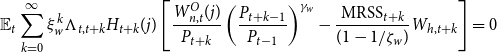 \begin{equation*} \mathbb {E}_t\sum _{k=0}^{\infty } \xi _w^k \Lambda _{t,t+k} H_{t+k}(j)\left [\frac {W_{n,t}^{O}(j)}{P_{t+k}} \left(\frac {P_{t+k-1}}{P_{t-1}}\right)^{\gamma _w}-\frac {\mbox {MRSS}_{t+k}}{(1-1/\zeta _w)} W_{h,t+k}\right ] =0 \end{equation*}
where we have introduced a mark-up shock $\mbox{MRSS}_t$
to the marginal rate of substitution that follows an AR1 process. This leads to
$\mbox{MRSS}_t$
to the marginal rate of substitution that follows an AR1 process. This leads to
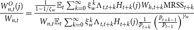 \begin{align*} \frac{W_{n,t}^{O}(j)}{W_{n,t}} &= \frac{\frac{1}{1-1/\zeta _w}\mathbb{E}_t\sum _{k=0}^{\infty } \xi _w^k \Lambda _{t,t+k}H_{t+k}(j)W_{h,t+k}\mbox{MRSS}_{t+k}}{W_{n,t} \mathbb{E}_t\sum _{k=0}^{\infty } \xi _w^k \Lambda _{t,t+k}H_{t+k}(j)\frac{1}{P_{t+k}}\left(\frac{P_{t+k-1}}{P_{t-1}}\right)^{\gamma _w}} \end{align*}
where $\frac{W_{n,t}^{O}(j)}{W_{n,t}}=\frac{W_{n,t}^{O}}{W_{n,t}}$
in a symmetric equilibrium.
$\frac{W_{n,t}^{O}(j)}{W_{n,t}}=\frac{W_{n,t}^{O}}{W_{n,t}}$
in a symmetric equilibrium.
By the law of large numbers the evolution of the aggregate wage is given by
 \begin{equation*} W_{n,t}^{1-\zeta _w} = \xi _w \left(W_{n,t-1}\Pi _{t-1}^{\gamma _w}\right)^{1-\zeta _w}+(1-\xi _w)(W_{n,t}^{O})^{1-\zeta _w } \end{equation*}
which can be written as
 \begin{equation} 1 = \xi _w \left(\frac{\Pi _{t-1}^{\gamma _w}}{\Pi _t^w}\right)^{1-\zeta _w}+(1-\xi _w)\left(\frac{W_{n,t}^O}{W_{n,t}}\right)^{1-\zeta _w} \end{equation}
Wage dispersion is defined as $\Delta _{w,t}=\int (W_{n,t}(j)/W_{n,t})^{-\zeta _w} dj$
. Assuming that the number of trade unions is large, we obtain the following dynamic relationship:
$\Delta _{w,t}=\int (W_{n,t}(j)/W_{n,t})^{-\zeta _w} dj$
. Assuming that the number of trade unions is large, we obtain the following dynamic relationship:
 \begin{align*} \Delta _{w,t} &= \xi _w\int _{not\ optimize} \left(\frac{W_{n,t-1}^O(j)\Pi _{t-1}^{\gamma _w}}{W_{n,t}}\right)^{-\zeta _w} dj + (1-\xi _w)\int _{optimize} \left(\frac{W_{n,t}^O(j)}{W_{n,t}}\right)^{-\zeta _w} dj \\ &= \xi _w \frac{(\Pi _t^w)^{\zeta _w}}{\Pi _{t-1}^{\zeta _w\gamma _w}} \Delta _{w,t-1}+(1-\xi _w)\left(\frac{W_{n,t}^O(j)}{W_{n,t}}\right)^{-\zeta _w} \end{align*}
3.3 Firms in the wholesale sector
Wholesale firms employ a Cobb–Douglas production function to produce a homogeneous output
 \begin{equation*} Y_t^W = F(A_t, H_t^d, u_t K_{t-1}) = (A_t H_t^d)^\alpha (u_tK_{t-1})^{1-\alpha } - F_t \end{equation*}
where $F_t$
are exogenous fixed costs growing in a balanced-growth steady in line with the other real variables. Profit-maximizing demand for factors results in the first order conditions
$F_t$
are exogenous fixed costs growing in a balanced-growth steady in line with the other real variables. Profit-maximizing demand for factors results in the first order conditions
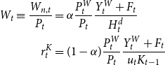 \begin{align*} W_t \equiv \frac{W_{n,t}}{P_t} &= \alpha \frac{P_t^W}{P_t}\frac{Y_t^W + F_t}{H_t^d} \\ r_t^K &= (1-\alpha ) \frac{P_t^W}{P_t}\frac{Y_t^W + F_t}{u_tK_{t-1}} \end{align*}
3.4 Firms in the retail sector
The retail sector uses a homogeneous wholesale good to produce a basket of differentiated goods for aggregate consumption
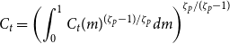 \begin{equation} C_{t}=\left( \int _{0}^{1}C_{t}(m)^{(\zeta _p -1)/\zeta _p }dm\right) ^{\zeta _p/(\zeta _p -1)} \end{equation}
where $\zeta _p$
is the elasticity of substitution. For each
$\zeta _p$
is the elasticity of substitution. For each $m$
, the consumer chooses
$m$
, the consumer chooses $C_t(m)$
at a price
$C_t(m)$
at a price $P_t(m)$
to maximize (19) given total expenditure
$P_t(m)$
to maximize (19) given total expenditure $\int _0^1 P_t(m) C_t(m) dm$
. This results in a set of consumption demand equations for each differentiated good
$\int _0^1 P_t(m) C_t(m) dm$
. This results in a set of consumption demand equations for each differentiated good $m$
with price
$m$
with price $P_{t}(m)$
of the form
$P_{t}(m)$
of the form
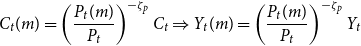 \begin{equation*} C_{t}(m)=\left( \frac {P_{t}(m)}{P_{t}}\right) ^{-\zeta _p }C_{t}\Rightarrow Y_{t}(m)=\left( \frac {P_{t}(m)}{P_{t}}\right) ^{-\zeta _p }Y_{t} \end{equation*}
where $P_{t}={\left [ \int _0^1 P_{t}(m)^{1-\zeta _p} dm \right ]}^{ \frac{1}{1-\zeta _p}}$
.
$P_{t}={\left [ \int _0^1 P_{t}(m)^{1-\zeta _p} dm \right ]}^{ \frac{1}{1-\zeta _p}}$
. $P_{t}$
is the aggregate price index.
$P_{t}$
is the aggregate price index. $C_t$
and
$C_t$
and $P_t$
are Dixit–Stigliz aggregates—see Dixit and Stiglitz (Reference Dixit and Stiglitz1977).
$P_t$
are Dixit–Stigliz aggregates—see Dixit and Stiglitz (Reference Dixit and Stiglitz1977).
Following Calvo (Reference Calvo1983), we now assume that there is a probability of $1-\xi _p$
at each period that the price of each retail good
$1-\xi _p$
at each period that the price of each retail good $m$
is set optimally to
$m$
is set optimally to $P_{t}^{0}(m)$
. If the price is not reoptimized, then prices are indexed to last period’s aggregate inflation, with indexation parameter
$P_{t}^{0}(m)$
. If the price is not reoptimized, then prices are indexed to last period’s aggregate inflation, with indexation parameter $\gamma _{p}$
. With indexation parameter
$\gamma _{p}$
. With indexation parameter $\gamma _p \geq 0$
, this implies that successive prices with no reoptimization are given by
$\gamma _p \geq 0$
, this implies that successive prices with no reoptimization are given by $P_{t}^{0}(f)$
,
$P_{t}^{0}(f)$
, $P_{t}^{0}(f)\left(\frac{P_{t}}{P_{t-1}}\right)^{\gamma _p}$
,
$P_{t}^{0}(f)\left(\frac{P_{t}}{P_{t-1}}\right)^{\gamma _p}$
, $P_{t}^{0}(f)\left(\frac{P_{t+1}}{P_{t-1}}\right)^{\gamma _p}$
,
$P_{t}^{0}(f)\left(\frac{P_{t+1}}{P_{t-1}}\right)^{\gamma _p}$
, $\ldots$
. For each retail producer
$\ldots$
. For each retail producer $m$
, given its real marginal cost (the inverse of the price mark-up)
$m$
, given its real marginal cost (the inverse of the price mark-up)
 \begin{equation*} MC_t=\frac {P_t^W}{P_t}, \end{equation*}
the objective is at time $t$
to choose
$t$
to choose $\{P_{t}^O(m)\}$
to maximize discounted profits
$\{P_{t}^O(m)\}$
to maximize discounted profits
 \begin{equation*} \mathbb {E}_t\sum _{k=0}^{\infty } \xi _p^k \Lambda _{t,t+k} Y_{t+k}(m) \left [\frac {P_{t}^{O}(m)}{P_{t+k}}\left(\frac {P_{t+k-1}}{P_{t-1}}\right)^{\gamma _p}- MC_{t+k}\right ] \end{equation*}
subject to
 \begin{equation*} Y_{t+k}(m)=\left [\frac {P_{t}^O(m)}{P_{t+k}}\left(\frac {P_{t+k-1}}{P_{t-1}}\right)^{\gamma _p}\right ] ^{-\zeta _p }Y_{t} \end{equation*}
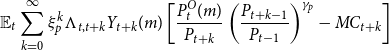
The solution to this is
 \begin{equation*} \mathbb {E}_t\sum _{k=0}^{\infty } \xi _p^k \Lambda _{t,t+k} Y_{t+k}(m)\left [\frac {P_{t}^{O}(m)}{P_{t+k}} \left(\frac {P_{t+k-1}}{P_{t-1}}\right)^{\gamma _p}-\frac {1}{(1-1/\zeta _p)} MC_{t+k}\right ] =0 \end{equation*}
which leads to
 \begin{equation*} \frac {P_{t}^{O}(m)}{P_t} = \frac {\frac {1}{1-1/\zeta _p}\mathbb {E}_t\sum _{k=0}^{\infty } \xi _p^k \Lambda _{t,t+k}\frac {\left(\frac {P_{t+k}}{P_{t}}\right)^{\zeta _p}}{\left(\frac {P_{t+k-1}}{P_{t-1}}\right)^{\gamma _p\zeta _p}}Y_{t+k}MC_{t+k}}{\mathbb {E}_t\sum _{k=0}^{\infty } \xi _p^k \Lambda _{t,t+k}\frac {\left(\frac {P_{t+k}}{P_{t}}\right)^{\zeta _p-1}}{\left(\frac {P_{t+k-1}}{P_{t-1}}\right)^{\gamma _p(\zeta _p-1)}}Y_{t+k}} \end{equation*}
where $\frac{P_{t}^{O}(m)}{P_t}=\frac{P_{t}^{O}}{P_t}$
in a symmetric equilibrium.
$\frac{P_{t}^{O}(m)}{P_t}=\frac{P_{t}^{O}}{P_t}$
in a symmetric equilibrium.
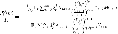
By the law of large numbers the evolution of the price index is given by
 \begin{equation*} P_{t}^{1-\zeta _p }=\xi _p \left(P_{t-1}\Pi _{t-1}^{\gamma _p}\right)^{1-\zeta _p}+(1-\xi _p)(P_{t}^{O}(m))^{1-\zeta _p } \end{equation*}
which can be written as
 \begin{equation*} 1 = \xi _p \left(\frac {\Pi _{t-1}^{\gamma _p}}{\Pi _t}\right)^{1-\zeta _p}+(1-\xi _p)\left(\frac {P_{t}^O(m)}{P_{t}}\right)^{1-\zeta _p} \end{equation*}
Price dispersion is defined as $\Delta _{p,t}=\int (P_t(m)/P_t)^{-\zeta _p} dm$
. Assuming that the number of firms is large, we obtain the following dynamic relationship:
$\Delta _{p,t}=\int (P_t(m)/P_t)^{-\zeta _p} dm$
. Assuming that the number of firms is large, we obtain the following dynamic relationship:
 \begin{align*} \Delta _{p,t} &= \xi _p \int _{not\ optimize} \left(\frac{P_{t-1}^O(m)\Pi _{t-1}^{\gamma _p}}{P_t}\right)^{-\zeta _p} dm + (1-\xi _w)\int _{optimize} \left(\frac{P_{t}^O(m)}{P_t}\right)^{-\zeta _p} dm \\ &= \xi _p \frac{\Pi _t^{\zeta _p}}{\Pi _{t-1}^{\zeta _p\gamma _p}} \Delta _{p,t-1}+(1-\xi _p)\left(\frac{P_t^O(m)}{P_t}\right)^{-\zeta _p} \end{align*}
3.5 Closing the model
The model is closed with a resource constraint
 \begin{equation*} Y_{t} = C_{t} + G_t + I_t + a(u_{t}) K_{t-1} \end{equation*}
A monetary policy rule for the nominal interest rate is given by the following Taylor-type rule
 \begin{align} \log \left( \frac{R_{n,t}}{R_n}\right) &= \rho _r \log \left( \frac{R_{n,t-1}}{R_n}\right) \nonumber \\ &\quad + (1-\rho _r)\left(\theta _{\pi } \log \left(\frac{\Pi _{t}}{\Pi }\right) + \theta _y \log \left(\frac{Y_t}{Y}\right) + \theta _{dy} \log \left(\frac{Y_t}{Y_{t-1}}\right)\right) \nonumber \\ &\quad + \log (MPS_t), \end{align}
where $MPS_t$
is a monetary policy shock and
$MPS_t$
is a monetary policy shock and $\rho _r \in [0,1]$
. Our rule is of the implementable form as proposed by Schmitt-Grohe and Uribe (Reference Schmitt-Grohe and Uribe2007) in that the nominal interest rate responds to deviations of output about its steady state rather than deviations about the flexi-price level of output (i.e., the output gap). The latter would encompass the original rules proposed by Taylor (Reference Taylor1993) and (Reference Taylor and Taylor1999) for which there is no interest-rate smoothing (
$\rho _r \in [0,1]$
. Our rule is of the implementable form as proposed by Schmitt-Grohe and Uribe (Reference Schmitt-Grohe and Uribe2007) in that the nominal interest rate responds to deviations of output about its steady state rather than deviations about the flexi-price level of output (i.e., the output gap). The latter would encompass the original rules proposed by Taylor (Reference Taylor1993) and (Reference Taylor and Taylor1999) for which there is no interest-rate smoothing ( $\rho _r=0$
) and
$\rho _r=0$
) and $\theta _{dy}=0$
. In the more recent of these papers, parameter values
$\theta _{dy}=0$
. In the more recent of these papers, parameter values $\theta _{\pi }=1.5$
and
$\theta _{\pi }=1.5$
and $\theta _{y}=1.0$
are proposed.Footnote
10
$\theta _{y}=1.0$
are proposed.Footnote
10
Nominal and real interest rates are related by the Fischer equation
 \begin{equation*} R_{t}=\left [ \frac {R_{n,t-1}}{\Pi _{t}} \right ] \end{equation*}
Market clearing for the labor market implies
 \begin{equation*} H_t = \int _0^1 H_t(j) dj= \int _0^1\left(\frac {W_{n,t}(j)}{W_{n,t}}\right)^{-\zeta _w} dj H_t^d= \Delta _{w,t} H_t^d \end{equation*}
Market clearing for the final good market implies
 \begin{equation*} Y_t^W = \Delta _{p,t} Y_t \end{equation*}
For completeness we include a government budget constraint
 \begin{align*} P_t G_t + B_{t-1} = T_t + \frac{B_t}{R_{n,t}} \end{align*}
where $G_t$
is government spending that follows an AR1 process. However, in this Ricardian set-up without distortionary taxes the constraint plays no role in the equilibrium.
$G_t$
is government spending that follows an AR1 process. However, in this Ricardian set-up without distortionary taxes the constraint plays no role in the equilibrium.
Finally, the seven exogenous processes are AR1 and evolve according to
 \begin{equation*} \log \Xi _t-\log \Xi =\rho _\Xi (\log \Xi _{t-1}-\log \Xi ) +\epsilon _{\Xi,t} \end{equation*}
where $\Xi =A,\,G,\,MS,\,MRSS,\,IS,\,RPS,\,MPS$
.
$\Xi =A,\,G,\,MS,\,MRSS,\,IS,\,RPS,\,MPS$
.
3.6 Departures from Smets and Wouters (Reference Smets and Wouters2007)
The following are features that differ from Smets and Wouters (Reference Smets and Wouters2007):
Kimball vs Dixit-Stiglitz aggregators: SW use Kimball aggregators with a super elasticity of $10$
. But empirical evidence by Klenow and Willis (Reference Klenow and Willis2016) suggests a much lower value which removes any discernable difference between the two (see Deak et al. (Reference Deak, Levine, Mirfatah and Swarbrick2023)). We therefore retain the Dixit–Stiglitz aggregators.
$10$
. But empirical evidence by Klenow and Willis (Reference Klenow and Willis2016) suggests a much lower value which removes any discernable difference between the two (see Deak et al. (Reference Deak, Levine, Mirfatah and Swarbrick2023)). We therefore retain the Dixit–Stiglitz aggregators.
Indexing and Trend Inflation: SW assume complete indexing in the steady state which removes all the trend inflation effects in our paper. We remove this assumption (see Ascari and Sbordone (Reference Ascari and Sbordone2014) for a discussion of indexation assumptions and the role of trend-inflation).
Shock Processes: We assume AR 1 shock processes throughout where SW assumes ARMA for inefficient mark-up shocks. Results are not sensitive to this assumption.
Sample Period: Estimation is over 1958:1–2017:4 and therefore unlike SW covers the ZLB period. We use the Mu-Xia shadow interest rate to replace the FEDFUNDs rate from 2009:1 onward intended to summarize the effects of unconventional monetary policy on private sector interest rates.
4. Bayesian estimation
This section sets out the Bayesian estimation of the model using standard techniques.Footnote 11 The model is linearized computationally about the nonzero net inflation positive growth deterministic state set out above. Before presenting the results, we first describe the measurement equations, the data, the methodology (briefly), and identification. We also highlight the information assumptions made in solving for a RE equilibrium that are usually only implicit in Bayesian estimation exercises.
The models of Smets and Wouters (Reference Smets and Wouters2007) are common and well known in this field. Especially, the Bayesian estimation result of the model is also available in the literature with standard data sample on the policy rate and sample length excluding the ZLB period (during the financial crisis and aftermath), which results in the smaller estimated shocks. However, our paper explores a different aspect, namely the ZLB constraint, the estimation of the model with a data sample taking the ZLB into consideration is neccessary. It is best to our knowledge that only Wu and Zhang (Reference Wu and Zhang2019) have done something similar by using the data sample with the shadow rate, but they did not consider the trend inflation in their estimation and the model they employed is much simpler than the standard Smets and Wouters (Reference Smets and Wouters2007) model.
4.1 Data and measurement equations
Our observables used in the estimation are: GDP per capita growth (dyobs), consumption expenditure per capita growth (dcobs), investment per capita growth (dinvobs), real wage growth (dwobs), percentage deviation of hours worked per capita from mean (labobs), monetary policy rate (robs), and inflation rate (pinfobs). The corresponding measurement equations expressed in terms of stationarized variablesFootnote 12 are
 \begin{align*} \mbox{dyobs} &= \log \left((1+g)\frac{Y_{t}}{Y_{t-1}}\right)\end{align*}
 \begin{align*} \mbox{dcobs} &= \log \left((1+g)\frac{C_{t}}{C_{t-1}}\right) \\ \mbox{dinvobs} &= \log \left((1+g)\frac{I_{t}}{I_{t-1}}\right) \\ \mbox{dwobs} &= \log \left((1+g)\frac{W_{t}}{W_{t-1}}\right) \\ \mbox{labobs} &= \frac{H_t^d - H^d}{H^d} \\ \mbox{robs} &= R_{n,t} - 1 \\ \mbox{pinfobs}&= \log \left(\Pi _t\right) \end{align*}
The steady-state values of the observables are dyobs=dinvobs=dcobs=dwobs= $\log (1+g)$
, labobs = 0, robs=
$\log (1+g)$
, labobs = 0, robs= $R_n-1$
, and pinfobs=
$R_n-1$
, and pinfobs= $\log (\Pi )$
.
$\log (\Pi )$
.
The original data are taken from the FRED Database available through the Federal Reserve Bank of St. Louis for the US economy. The data consists of 7 quarterly time series, namely log output growth ( $dyobs$
), log consumption growth (
$dyobs$
), log consumption growth ( $dcobs$
), log investment growth (
$dcobs$
), log investment growth ( $dinvobs$
), log wage growth (
$dinvobs$
), log wage growth ( $dwobs$
), labor hours supply (
$dwobs$
), labor hours supply ( $labobs$
), the net inflation (
$labobs$
), the net inflation ( $pinfobs$
), and finally the policy rate measurement (
$pinfobs$
), and finally the policy rate measurement ( $robs$
), because our focus on the ZLB we provide an estimation with the Wu-Xia Shadow interest rate replacing the FEDFUNDS rate,
$robs$
), because our focus on the ZLB we provide an estimation with the Wu-Xia Shadow interest rate replacing the FEDFUNDS rate, $robs$
—see Wu & Xia, Reference Wu and Xia2016). The sample period is 1958:1–2017:4. There is a presample period of 4 quarters so the observations actually used for the estimation go from 1959:1-2017:4, 240 observations (Table 1).
$robs$
—see Wu & Xia, Reference Wu and Xia2016). The sample period is 1958:1–2017:4. There is a presample period of 4 quarters so the observations actually used for the estimation go from 1959:1-2017:4, 240 observations (Table 1).
Table 1. St. Louis FRED original data

We then calculate the log growth rates of output ( $dyobs$
), consumption (
$dyobs$
), consumption ( $dcobs$
), investment (
$dcobs$
), investment ( $dinvobs$
), and wage (
$dinvobs$
), and wage ( $dwobs$
) by taking the first difference of
$dwobs$
) by taking the first difference of $yobs$
,
$yobs$
, $cobs$
,
$cobs$
, $invobs$
, and
$invobs$
, and $wobs$
, respectively. The shadow Federal Funds Rate data are taken from the Federal reserve Bank of Atlanta. Wu & Xia (Reference Wu and Xia2016) propose a simple analytical representation for bond prices in the multifactor shadow rate term structure model. Unlike the observed short-term interest rate, the shadow rate is not bounded below by 0 percent. Whenever the Wu-Xia shadow rate is above 0.25% per annum (approximately 0.25/4% per quarter), it is exactly equal to the Federal Funds Effective Rate (FEDFUNDS). The model proposed in Wu & Xia Reference Wu and Xia(2016) summarizes the macroeconomic effects of unconventional monetary policy, that is, at the ZLB of the nominal interest rate. Common literature focused on measuring the effects on the yield curve, but this posed a challenge to measure the relations between the yields on assets of different maturities in the new environment, that is, during the ZLB period where the unconventional monetary policy is implemented. Therefore, the multifactor shadow rate term structure model offers a better empirical description of the behavior of interest rates during the ZLB period.
$wobs$
, respectively. The shadow Federal Funds Rate data are taken from the Federal reserve Bank of Atlanta. Wu & Xia (Reference Wu and Xia2016) propose a simple analytical representation for bond prices in the multifactor shadow rate term structure model. Unlike the observed short-term interest rate, the shadow rate is not bounded below by 0 percent. Whenever the Wu-Xia shadow rate is above 0.25% per annum (approximately 0.25/4% per quarter), it is exactly equal to the Federal Funds Effective Rate (FEDFUNDS). The model proposed in Wu & Xia Reference Wu and Xia(2016) summarizes the macroeconomic effects of unconventional monetary policy, that is, at the ZLB of the nominal interest rate. Common literature focused on measuring the effects on the yield curve, but this posed a challenge to measure the relations between the yields on assets of different maturities in the new environment, that is, during the ZLB period where the unconventional monetary policy is implemented. Therefore, the multifactor shadow rate term structure model offers a better empirical description of the behavior of interest rates during the ZLB period.
4.2 Identification and information assumptions
It is necessary to confront the question of parameter identifiability in DSGE models before taking them to the data, as model or parameter identification is a prerequisite for the informativeness of different estimators, and their effectiveness when one uses the models to address policy questions. Hence, we follows Iskrev (Reference Iskrev2010), Iskrev and Ratto (Reference Iskrev and Ratto2010) to perform formal identification checks on the reduced form parameters and structure or deep parameters. Overall, our identification analysis using dynare Dynare (2023) shows that the Jacobian and Hessian matrices of the mapping from the reduced form of the estimated parameters into the first and second order moments of the observable variables are full rank. Thus, our estimated model is locally identifiable given the priors and observable data sample. Details of this analysis are shown in the Online Appendix.
There is one more issue to address regarding the assumed information set of the agents in the model. Most DSGE models are still solved and/or estimated on the assumption that agents are simply provided with perfect information (henceforth PI) regarding the states including the exogenous processes, effectively as an endowment. If we drop this implausible assumption we must consider a signal extraction problem under imperfect information (II) for the agents in the model analogous to that we have considered for the econometrician. Fortunately we can retain the PI solution if we restrict ourselves to a class of models which are ‘A-invertible’ meaning that agents can infer the structural shocks from the information set assumed to be that of the econometrician. Levine et al. (Reference Levine, Pearlman, Wright and Yang2019) provide an A-invertibility condition that generalizes the “Poor Man’s Invertibility Condition” of Fernandez-Villaverde et al. (Reference Fernandez-Villaverde, Rubio-Ramirez, Sargent and Watson2007) and show that in the Smets and Wouters (Reference Smets and Wouters2007) of this paper with seven shock processes and seven observables is indeed A-invertible.Footnote 13 It follows that II and PI solutions coincide and the standard information assumption is valid in our model.
4.3 Estimation results
Table 2 indicates the priors, the estimated posterior mode of the parameters obtained directly from the maximization of the posterior distribution, and the mean of the posterior distribution of the parameters obtained through the Metropolis–Hastings sampling algorithm of our estimation.Footnote 14 The priors on the stochastic processes are identical to Smets and Wouters (Reference Smets and Wouters2007). The standard errors of the innovations are assumed to follow an inverse-gamma distribution with a mean of 0.001 (Smets and Wouters (Reference Smets and Wouters2007) use unscaled data with mean priors at 0.1) and 0.02 degrees of freedom (2 in Smets and Wouters (Reference Smets and Wouters2007)), which corresponds to a rather loose prior. The persistence of the AR(1) processes is beta distributed with mean 0.5 and standard error 0.2. Unlike Smets and Wouters (Reference Smets and Wouters2007) who estimated the trend growth with normal distribution of mean 0.4% and standard deviation of 0.1, we fix this trend growth at the empirical value of 0.355%. We also empirically calibrate the steady state of inflation, discount factor, and steady state of shadow interest rate by using the sample data.
Table 2. Estimated results (posterior mean with a number of draws equal to 100,000)
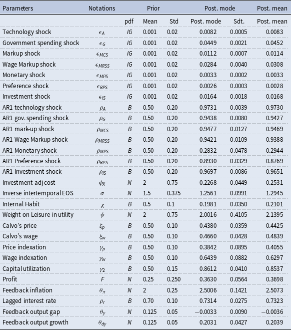
The parameters describing the monetary policy rule are based on a standard Taylor rule: the long run reaction on inflation and the output gap are described by a normal distribution with mean 2.0 and 0.125 (0.5 divided by 4) and standard errors 0.25 and 0.05, respectively. The persistence of the policy rule is determined by the coefficient on the lagged interest rate rate, which is assumed to be Beta distribution with mean of 0.75 with a standard error of 0.1. The prior on the short run reaction coefficient to the change in the output growth is normal distribution with mean 0.125 standard error 0.05.
The parameters of the utility function are assumed to be distributed as follows: the intertemporal elasticity of substitution is set at 1.5 with a standard error of 0.375; the habit parameter is assumed to fluctuate around 0.5 with a standard error of 0.1 and the elasticity of labor supply is assumed to be around 2 with a standard error of 0.75. These are all quite standard calibrations. The prior on the adjustment cost parameter for investment is set around 2 with a standard error of 0.75 and the capacity utilization elasticity is set at 0.5 with a standard error of 0.15. The share of fixed costs in the production function is assumed to have a prior mean of 0.25. Finally, there are the parameters describing the price and wage setting. The Calvo probabilities are assumed to be around 0.5 for both prices and wages, suggesting an average length of price and wage contracts of half a year. The prior mean of the degree of indexation to past inflation is also set at 0.5 in both goods and labor markets. These priors are standard as in Smets and Wouters (Reference Smets and Wouters2007).
Overall, all estimated parameters are significantly different from zero. Most of the persistent shocks are estimated to have an autoregressive parameter that lies above 0.9, with the exception of the estimated persistent parameter on monetary policy shock standing at 0.31. In addition, we find that the estimated price indexation parameter is smaller than the mean assumed in their prior distribution, $\gamma _p = 0.40$
, but wage indexation is higher at
$\gamma _p = 0.40$
, but wage indexation is higher at $\gamma _w = 0.63$
. Moreover, the estimated Calvo’s price and wage parameters are relatively small at
$\gamma _w = 0.63$
. Moreover, the estimated Calvo’s price and wage parameters are relatively small at $\xi _p = 0.44$
and
$\xi _p = 0.44$
and $\xi _w = 0.48$
, but taken together these estimates represent a significant degree of price and wage stickiness and departure from full indexation. Thus, a positive trend inflation leads to a significant welfare cost owing to both steady state and dynamic costs discussed in Section 2.1. Besides, other estimated parameters’ values are consistent with the results from Smets and Wouters (Reference Smets and Wouters2007). However, our estimated parameters on price and wage rigidity are slightly smaller than that in Smets and Wouters (Reference Smets and Wouters2007). The difference in estimation results comes from the data sample used, for example, in this study, we considered the full sample of the ZLB period with shadow rate rather than the nominal interest rate up to 2017. Another feature comes from the aggregator adopted in the price-setting problem; in our study we use the Dixit–Stiglitz aggregator while Smets and Wouters (Reference Smets and Wouters2007) uses the Kimball aggregator. For our full sample data (from 1947 to 2017) comparing to Smets and Wouters (Reference Smets and Wouters2007) (from 1966 to 2004), our sample data contain the more volatile inflation and wage periods, which results in a lower level price and wage rigidity levels. In addition, our estimated shocks are higher in magnitude comparing to that in Smets and Wouters (Reference Smets and Wouters2007), again this mainly results from our choice of sample data covering the financial crisis and aftermath periods, where we use the shadow policy rate which took negative values during these periods, that is, a highly volatile economy, transferred into a higher level of shocks.
$\xi _w = 0.48$
, but taken together these estimates represent a significant degree of price and wage stickiness and departure from full indexation. Thus, a positive trend inflation leads to a significant welfare cost owing to both steady state and dynamic costs discussed in Section 2.1. Besides, other estimated parameters’ values are consistent with the results from Smets and Wouters (Reference Smets and Wouters2007). However, our estimated parameters on price and wage rigidity are slightly smaller than that in Smets and Wouters (Reference Smets and Wouters2007). The difference in estimation results comes from the data sample used, for example, in this study, we considered the full sample of the ZLB period with shadow rate rather than the nominal interest rate up to 2017. Another feature comes from the aggregator adopted in the price-setting problem; in our study we use the Dixit–Stiglitz aggregator while Smets and Wouters (Reference Smets and Wouters2007) uses the Kimball aggregator. For our full sample data (from 1947 to 2017) comparing to Smets and Wouters (Reference Smets and Wouters2007) (from 1966 to 2004), our sample data contain the more volatile inflation and wage periods, which results in a lower level price and wage rigidity levels. In addition, our estimated shocks are higher in magnitude comparing to that in Smets and Wouters (Reference Smets and Wouters2007), again this mainly results from our choice of sample data covering the financial crisis and aftermath periods, where we use the shadow policy rate which took negative values during these periods, that is, a highly volatile economy, transferred into a higher level of shocks.
5. The delegation game
We now turn to ZLB considerations. Before considering transparent simple quadratic mandates, we first examine the numerical solution of the two-stage delegation game in the estimated SW model in the case where the choice of response parameters $\rho$
is delegated to a central bank with a ‘modified’ objective of the form (21) where
$\rho$
is delegated to a central bank with a ‘modified’ objective of the form (21) where $U_{t}$
is household utility and the rule takes the form (29). The equilibrium of this ZLB delegation mandate is solved by backward induction in the following two-stage game 1.
$U_{t}$
is household utility and the rule takes the form (29). The equilibrium of this ZLB delegation mandate is solved by backward induction in the following two-stage game 1.
Stage 1: The Government (the leader) chooses a per period probability of hitting the ZLB, a trend inflation rate and designs the optimal loss function in the mandate. The optimal steady-state inflation rate consistent with stage 1 is chosen also by the Government 2.
Stage 2: The CB (the follower) receives the mandate in the form of a modified purely stochastic welfare criterion of the form $\Omega_{t}(\mathsf{Z}, \Pi, \rho) $
of the form (4) with an additional penalty to limit the variance of the nominal interest rate rule. Welfare is then optimized with respect to
$\Omega_{t}(\mathsf{Z}, \Pi, \rho) $
of the form (4) with an additional penalty to limit the variance of the nominal interest rate rule. Welfare is then optimized with respect to $ \rho \in S $
resulting in an optimized simple rule.
$ \rho \in S $
resulting in an optimized simple rule.
This delegation game is solved by backward induction as follows:
5.1. Stage 2: The CB choice of rule
Given a steady-state inflation rate target, $\Pi$
, the Central Bank (CB) receives a mandate to implement the rule (29) and to maximize with respect to
$\Pi$
, the Central Bank (CB) receives a mandate to implement the rule (29) and to maximize with respect to $\rho \in S$
a modified welfare criterion
$\rho \in S$
a modified welfare criterion
 \begin{equation} \Omega _t^{mod} \equiv \mathbb{E}_t\left [ \sum _{\tau =0}^\infty \beta ^{\tau } \left(U_{t+\tau } - w_r \left(R_{n,t+\tau } - R_n \right)^2 \right)\right ]=\left(U_{t} - w_r \left(R_{n,t} - R_n \right)^2 \right)+ \beta \mathbb{E}_t \left [ \Omega _{t+1}^{mod} \right ] \end{equation}
in a zero-growth steady state with $g=0$
. To be consistent with our estimated model with
$g=0$
. To be consistent with our estimated model with $g\gt 0$
, we use a stationarized form:
$g\gt 0$
, we use a stationarized form:
 \begin{equation} \Omega _t^{mod} =\left(U_{t} - w_r \left(R_{n,t} - R_n \right)^2 \right)+ \beta (1+g)^{1-\sigma }\mathbb{E}_t \left [ \Omega _{t+1}^{mod} \right ] \end{equation}
Details of this stationary form are given in the Online Appendix B.1. One can think of this formulation as a mandate with a choice of penalty function $P=w_r \left(R_{n,t} - R_n \right)^2$
, penalizing the variance of the nominal interest rate with weight
$P=w_r \left(R_{n,t} - R_n \right)^2$
, penalizing the variance of the nominal interest rate with weight $w_r$
that is chosen at Stage 1 of the game.Footnote
15
$w_r$
that is chosen at Stage 1 of the game.Footnote
15
Following Den Haan and Wind (Reference Den Haan and Wind2012), an alternative mandate that only penalizes the zero interest rate in an asymmetric fashion is $P=P(a_t)$
where the occasionally binding constraint is
$P=P(a_t)$
where the occasionally binding constraint is $a_t \equiv R_{n,t}-1 \ge 0$
with
$a_t \equiv R_{n,t}-1 \ge 0$
with
 \begin{equation} P=P(a_t)= \frac{\exp (-w_r a_t)}{w_r} \end{equation}
and chooses a large $w_r$
.
$w_r$
. $P(a_t)$
then has the property
$P(a_t)$
then has the property
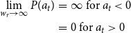 \begin{eqnarray*} \lim _{w_r \rightarrow \infty } P(a_t) &=& \infty \mbox{ for } a_t\lt 0\\ &=& 0 \mbox{ for } a_t\gt 0 \end{eqnarray*}
Thus, $P(a_t)$
enforces the ZLB approximately but with more accuracy as
$P(a_t)$
enforces the ZLB approximately but with more accuracy as $w_r$
becomes large. Stages 2–1 then proceed as before, but we now confine ourselves to a large
$w_r$
becomes large. Stages 2–1 then proceed as before, but we now confine ourselves to a large $w_r$
which will enable
$w_r$
which will enable $\Pi$
to be close to unity.
$\Pi$
to be close to unity.
Both the symmetric and asymmetric forms of a ZLB mandate result in a probability of hitting the ZLB
 \begin{equation} p=p(\Pi, \rho ^*(\Pi, w_r)) \end{equation}
where $\rho ^*(\Pi, w_r)$
is the optimized form of the rule given the steady-state target
$\rho ^*(\Pi, w_r)$
is the optimized form of the rule given the steady-state target $\Pi$
and the weight on the interest rate volatility,
$\Pi$
and the weight on the interest rate volatility, $w_r$
.
$w_r$
.
5.2 Stage 1: Design of the mandate
The Government first chooses a per period probability $\bar{p}_{zlb}$
of the nominal interest rate hitting the ZLB (which defines the tightness of the ZLB constraint). Given this target low probability and given
$\bar{p}_{zlb}$
of the nominal interest rate hitting the ZLB (which defines the tightness of the ZLB constraint). Given this target low probability and given $w_r$
,
$w_r$
, $\Pi =\Pi ^*$
is chosen to satisfy
$\Pi =\Pi ^*$
is chosen to satisfy
 \begin{equation} p(R_{n,t} \leq 1) \equiv p(\Pi ^*, \rho ^*(\Pi ^*, w_r)) \leq \bar{p}_{zlb} \end{equation}
This then achieves the ZLB constraint
 \begin{equation} R_{n,t} \geq 1 \mbox{ with probability } ( 1 - \bar{p}_{zlb}) \end{equation}
where $R_{n,t}$
is the nominal interest rate.
$R_{n,t}$
is the nominal interest rate.
The leader then maximizes the actual household intertemporal welfare
 \begin{eqnarray} \Omega _t=\mathbb{E}_t\left [ \sum _{\tau =0}^\infty \beta ^{\tau } U_{t+\tau }\right ]= U_t+\beta (1+g)^{1-\sigma }\mathbb{E}_t \left [ \Omega _{t+1} \right ] \end{eqnarray}
with respect to $w_r$
.
$w_r$
.
This two-stage delegation game defines an equilibrium in choice variables $w_r^*$
,
$w_r^*$
, $\rho ^*$
, and
$\rho ^*$
, and $\Pi ^*$
given
$\Pi ^*$
given $\bar{p}_{zlb}$
that maximizes the actual household welfare subject to the ZLB constraint (26). It should be noted at this point that the Ramsey Optimum maximizes
$\bar{p}_{zlb}$
that maximizes the actual household welfare subject to the ZLB constraint (26). It should be noted at this point that the Ramsey Optimum maximizes $\Omega _t$
given by (27) subject only to the constraints of the model, but with no ZLB concerns. As is standard in models such as ours it results in a zero net inflation (
$\Omega _t$
given by (27) subject only to the constraints of the model, but with no ZLB concerns. As is standard in models such as ours it results in a zero net inflation ( $\Pi =1$
).
$\Pi =1$
).
5.3 Welfare-optimal simple rules
The concept and computation of optimized simple rules in an estimated model is central to this paper. We first make some general points before turning to the full delegation game and the results. We follow Schmitt-Grohe and Uribe (Reference Schmitt-Grohe and Uribe2007) quite closely, but with some important differences.
First recall the form of the estimated nominal interest rate rule:
 \begin{align} \log \left( \frac{R_{n,t}}{R_n}\right) & =\rho _r \log \left( \frac{R_{n,t-1}}{R_n}\right) +(1-\rho _r)\left(\theta _\pi \log \left(\frac{\Pi _{t}}{\Pi }\right) + \theta _y \log \left(\frac{Y_t}{Y}\right) + \theta _{dy} \log \left(\frac{Y_t}{Y_{t-1}}\right)\right) \nonumber \\ & \quad + \log (MPS_t) \end{align}
Unlike rules studied in the NK literature that respond to the output gap and therefore a fully flexible price version of the model, this rule makes no such demands on the central bank and rational agents; it only requires knowledge of the model itself and its deterministic steady state. Schmitt-Grohe and Uribe (Reference Schmitt-Grohe and Uribe2007) refer to such rules as “implementable.”
For optimal policy purposes, we remove the monetary policy shock $\log (MPS_t)$
and reparameterize the rule as
$\log (MPS_t)$
and reparameterize the rule as
 \begin{equation} \log \left( \frac{R_{n,t}}{R_n}\right)=\rho _r \log \left( \frac{R_{n,t-1}}{R_n}\right) +\alpha _\pi \log \left(\frac{\Pi _{t}}{\Pi }\right) + \alpha _y \log \left(\frac{Y_t}{Y}\right) + \alpha _{dy} \log \left(\frac{Y_t}{Y_{t-1}}\right) \end{equation}
which allows for the possibility of an integral rule with $\rho _r=1$
. Let
$\rho _r=1$
. Let $\rho \equiv [ \rho _r, \alpha _\pi, \alpha _y, \alpha _{dy}]$
be the policy choice of feedback parameters that defines the exact form of the rule. We restrict ourselves to a class of possible rules that are locally saddle-path stable in the vicinity of the non-stochastic (deterministic) steady state. We denote this subset of rules by
$\rho \equiv [ \rho _r, \alpha _\pi, \alpha _y, \alpha _{dy}]$
be the policy choice of feedback parameters that defines the exact form of the rule. We restrict ourselves to a class of possible rules that are locally saddle-path stable in the vicinity of the non-stochastic (deterministic) steady state. We denote this subset of rules by $S$
; thus
$S$
; thus $\rho \in S$
.
$\rho \in S$
.
Two forms of rule found in the literature are special cases of (29). First, put $\rho _r=1$
and
$\rho _r=1$
and $\alpha _{dy}=\alpha _{y}=0$
to give
$\alpha _{dy}=\alpha _{y}=0$
to give
 \begin{equation} \log \left( \frac{R_{n,t}}{R_n}\right)=\log \left( \frac{R_{n,t-1}}{R_n}\right) +\alpha _\pi \log \left(\frac{\Pi _{t}}{\Pi }\right) \end{equation}
Then integrating we arrive at
 \begin{equation} \log \left( \frac{R_{n,t}}{R_n}\right)=\alpha _\pi \log \left(\frac{P_{t}}{\bar{P}_t}\right) \end{equation}
which is a price level rule with the trend price-level given by $\frac{\bar{P}_t}{\bar{P}_{t-1}}=\Pi _t$
. The benefits of price-level targeting versus inflation targeting have been discussed in the literature review subsection of the Introduction. The intuition for the benefits of price-targeting is as follows: faced with an unexpected temporary rise in inflation, price-level stabilization commits the central bank to bring inflation below the target in subsequent periods. In contrast, with inflation targeting, the drift in the price level is accepted.Footnote
16
$\frac{\bar{P}_t}{\bar{P}_{t-1}}=\Pi _t$
. The benefits of price-level targeting versus inflation targeting have been discussed in the literature review subsection of the Introduction. The intuition for the benefits of price-targeting is as follows: faced with an unexpected temporary rise in inflation, price-level stabilization commits the central bank to bring inflation below the target in subsequent periods. In contrast, with inflation targeting, the drift in the price level is accepted.Footnote
16
We begin by defining the intertemporal household welfare at time $t$
in recursive Bellman stationarized formFootnote
17
in a symmetric equilibrium form as:
$t$
in recursive Bellman stationarized formFootnote
17
in a symmetric equilibrium form as:
 \begin{eqnarray} \Omega _t &=&U_t(C_t, C_{t-1}, H_t^s) +\beta _{g} \mathbb{E}_t \left [ \Omega _{t+1}\right ] \end{eqnarray}
where $\beta _{g}$
is a growth-adjusted discount factor defined by
$\beta _{g}$
is a growth-adjusted discount factor defined by $\beta _g \equiv \beta (1+g)^{1-\sigma }$
.
$\beta _g \equiv \beta (1+g)^{1-\sigma }$
. $\Omega _t$
is a function of policy,
$\Omega _t$
is a function of policy, $R_{n,t}$
and all the estimated parameters in the model including those for the AR1 shocks processes. We take the latter dependence as given in what follows.
$R_{n,t}$
and all the estimated parameters in the model including those for the AR1 shocks processes. We take the latter dependence as given in what follows.
Given initial values for the predetermined variables, $\mathsf{Z}_0$
, optimal policy at time
$\mathsf{Z}_0$
, optimal policy at time $t=0$
sets steady-state values for the nominal interest rate instrument
$t=0$
sets steady-state values for the nominal interest rate instrument $R_{n,t}$
, denoted by
$R_{n,t}$
, denoted by $R_n$
(which should be noted depends on the steady-state inflation target) and solves the maximization problem:
$R_n$
(which should be noted depends on the steady-state inflation target) and solves the maximization problem:
 \begin{align} \max _{\rho \in S} \Omega _0 ( \mathsf{Z}_0, R_n, \rho ) \end{align}
In fact the long-run (steady state) gross inflation rate target in the rule which we take to be $\Pi \ge 1$
(ruling out a liquidity trap) uniquely pins down the rest of the steady state so we can rewrite (33) as
$\Pi \ge 1$
(ruling out a liquidity trap) uniquely pins down the rest of the steady state so we can rewrite (33) as
 \begin{align} \max _{\rho \in S} \Omega _0 ( \mathsf{Z}_0, \Pi, \rho ) \end{align}
But this is a conditional and time-inconsistent criterion as the optimized rule at time $t$
becomes
$t$
becomes
 \begin{equation} \max _{\rho \in S} \Omega _t ( \mathsf{Z}_t, \Pi, \rho ) \Rightarrow \rho =\rho ( \mathsf{Z}_t, \Pi ) \end{equation}
At time $t=0$
optimal commitment is to the optimized rule and depends on
$t=0$
optimal commitment is to the optimized rule and depends on $\mathsf{Z}_0$
. But with the mere passage of time reoptimization (in the absence of commitment) becomes a dependence on
$\mathsf{Z}_0$
. But with the mere passage of time reoptimization (in the absence of commitment) becomes a dependence on $\mathsf{Z}_t$
and this leads to an incentive to reoptimize (i.e., time inconsistency).
$\mathsf{Z}_t$
and this leads to an incentive to reoptimize (i.e., time inconsistency).
We remove one source of time-inconsistency by choosing a welfare conditional on the economy being at the steady state $\mathsf{Z}_t=\mathsf{Z}$
, which is exogenous and policy-invariant. But welfare is also conditional the steady-state inflation target,
$\mathsf{Z}_t=\mathsf{Z}$
, which is exogenous and policy-invariant. But welfare is also conditional the steady-state inflation target, $\Pi$
, which is a policy choice leaving a well-known source of time-inconsistency arising from the incentive to engage in an inflation surprise.Footnote
18
The optimization problem then becomes
$\Pi$
, which is a policy choice leaving a well-known source of time-inconsistency arising from the incentive to engage in an inflation surprise.Footnote
18
The optimization problem then becomes
 \begin{equation} \max _{\rho \in S} \Omega ( \mathsf{Z}, \Pi, \rho ) \Rightarrow \rho =\rho ( \mathsf{Z}, \Pi ) \end{equation} $\Omega$
is now time-invariant and since
$\Omega$
is now time-invariant and since $\mathsf{Z}$
is policy-invariant, in what follows we simply write
$\mathsf{Z}$
is policy-invariant, in what follows we simply write $\rho =\rho (\Pi )$
. Since the steady-state inflation target
$\rho =\rho (\Pi )$
. Since the steady-state inflation target $\Pi$
is a policy choice chosen in the mandate a commitment to this particular value is the remaining source of time-inconsistency. Thus welfare at the steady state is maximized on average over all realizations of future shocks driving the exogenous stochastic processes given their deterministic steady states. The optimal rule
$\Pi$
is a policy choice chosen in the mandate a commitment to this particular value is the remaining source of time-inconsistency. Thus welfare at the steady state is maximized on average over all realizations of future shocks driving the exogenous stochastic processes given their deterministic steady states. The optimal rule $\rho ^*$
is computed using a second-order perturbation solution.Footnote
19
But there are no ZLB considerations for the nominal interest rate as yet. This leads us to the delegation game.
$\rho ^*$
is computed using a second-order perturbation solution.Footnote
19
But there are no ZLB considerations for the nominal interest rate as yet. This leads us to the delegation game.
6. The ZLB delegation mandate: Numerical results
We now turn to the numerical solution of the two-stage delegation game starting at Stage 2.
6.1. Stage 2 of the delegation game
At Stage 2, the central bank at time $t$
is instructed to maximize
$t$
is instructed to maximize $\Omega _t^{mod}$
with respect to the feedback coefficients
$\Omega _t^{mod}$
with respect to the feedback coefficients $\rho \equiv [ \rho _r, \alpha _\pi, \alpha _y, \alpha _{dy}]$
given the long-run inflation target
$\rho \equiv [ \rho _r, \alpha _\pi, \alpha _y, \alpha _{dy}]$
given the long-run inflation target $\Pi =\Pi ^*$
and the weight
$\Pi =\Pi ^*$
and the weight $w_r$
. Note that the CB takes the weight
$w_r$
. Note that the CB takes the weight $w_r$
(presenting the objective function of the CB) and the steady state of inflation as given to find the optimized feedback rule. Therefore, in the exercise of the Stage 2, we simply run the optimized feedback (simple) rule on nominal interest rate for each given pair of
$w_r$
(presenting the objective function of the CB) and the steady state of inflation as given to find the optimized feedback rule. Therefore, in the exercise of the Stage 2, we simply run the optimized feedback (simple) rule on nominal interest rate for each given pair of $(w_r, \Pi )$
. The upper-left subplot of Fig. 2 shows the relationship between the ZLB probability for each value of the gross steady-state inflation rate. In particular, the probability of hitting the ZLB is a decreasing function in the level of the inflation target (see CGW, Ngo (Reference Ngo2018)), that is, given the same value of the weight
$(w_r, \Pi )$
. The upper-left subplot of Fig. 2 shows the relationship between the ZLB probability for each value of the gross steady-state inflation rate. In particular, the probability of hitting the ZLB is a decreasing function in the level of the inflation target (see CGW, Ngo (Reference Ngo2018)), that is, given the same value of the weight $w_r$
, the probability of hitting the ZLB moves from the dashed down to the solid lines associating with an increasing of inflation from
$w_r$
, the probability of hitting the ZLB moves from the dashed down to the solid lines associating with an increasing of inflation from $1.00$
to
$1.00$
to $1.009$
(dashed-o and dashed-x lines express the inflation levels of
$1.009$
(dashed-o and dashed-x lines express the inflation levels of $1.003$
–
$1.003$
– $1.006$
, respectively).
$1.006$
, respectively).
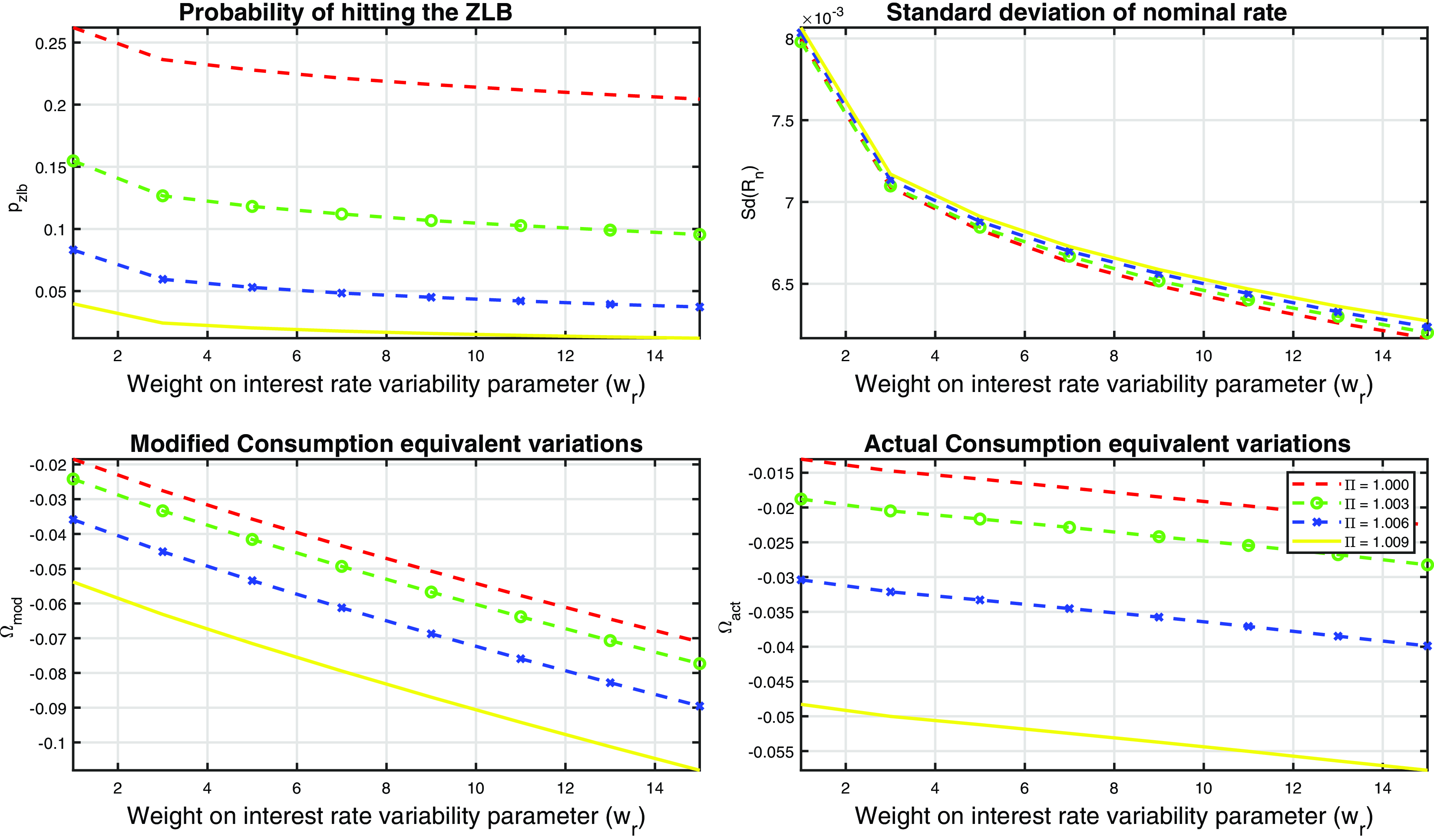
Figure 2. Plots of the probability of hitting the ZLB, the standard deviation of the instrument rate and the welfare criteria to the weight on interest rate variability parameter, $w_r$
(x-axis), and for different steady-state inflation levels (dashed to solid lines).
$w_r$
(x-axis), and for different steady-state inflation levels (dashed to solid lines).
However, increasing the inflation target has two opposite effects on the probability of hitting the ZLB: the first is on the first moment by shifting the density function to the right reducing the probability of hitting ZLB; the second effect is on the second moment making the shape of the density function more fat-tailed. The upper-right subplot shows this second effect: namely that the standard deviation of the nominal rate is an increasing function of the inflation target thus increasing the probability of hitting ZLB. As shown from the upper-left subplot, the probability of hitting the ZLB is a decreasing function of the steady-state inflation, or the first effect dominates the second effect in this model.
From the lower-right subplot of Fig. 2, we can see that actual consumption equivalent variation (or actual welfare criterion) is a decreasing function in the inflation target. There are two remarks on this: first, if the ZLB is not taken into account, the optimal rate of gross inflation is one (or net inflation is zero) because there are only costs to inflation and no required shifting of the inflation rate; second, considering the set of all the steady-state inflation levels which satisfies the ZLB (the red arrow in Fig. 3), $\Pi ^* \geq \Pi ^{**} = 1.005$
, the policymaker chooses the target inflation of
$\Pi ^* \geq \Pi ^{**} = 1.005$
, the policymaker chooses the target inflation of $\Pi ^{**} = 1.005$
with a given value of
$\Pi ^{**} = 1.005$
with a given value of $w_r = 1$
and
$w_r = 1$
and $\bar{p}_{zlb} = 0.103$
(approx.
$\bar{p}_{zlb} = 0.103$
(approx. $0.1$
). In other words, given a set of inflation target levels that satisfy the ZLB constraint, the lowest inflation target level is always chosen to maximize the actual welfare.
$0.1$
). In other words, given a set of inflation target levels that satisfy the ZLB constraint, the lowest inflation target level is always chosen to maximize the actual welfare.
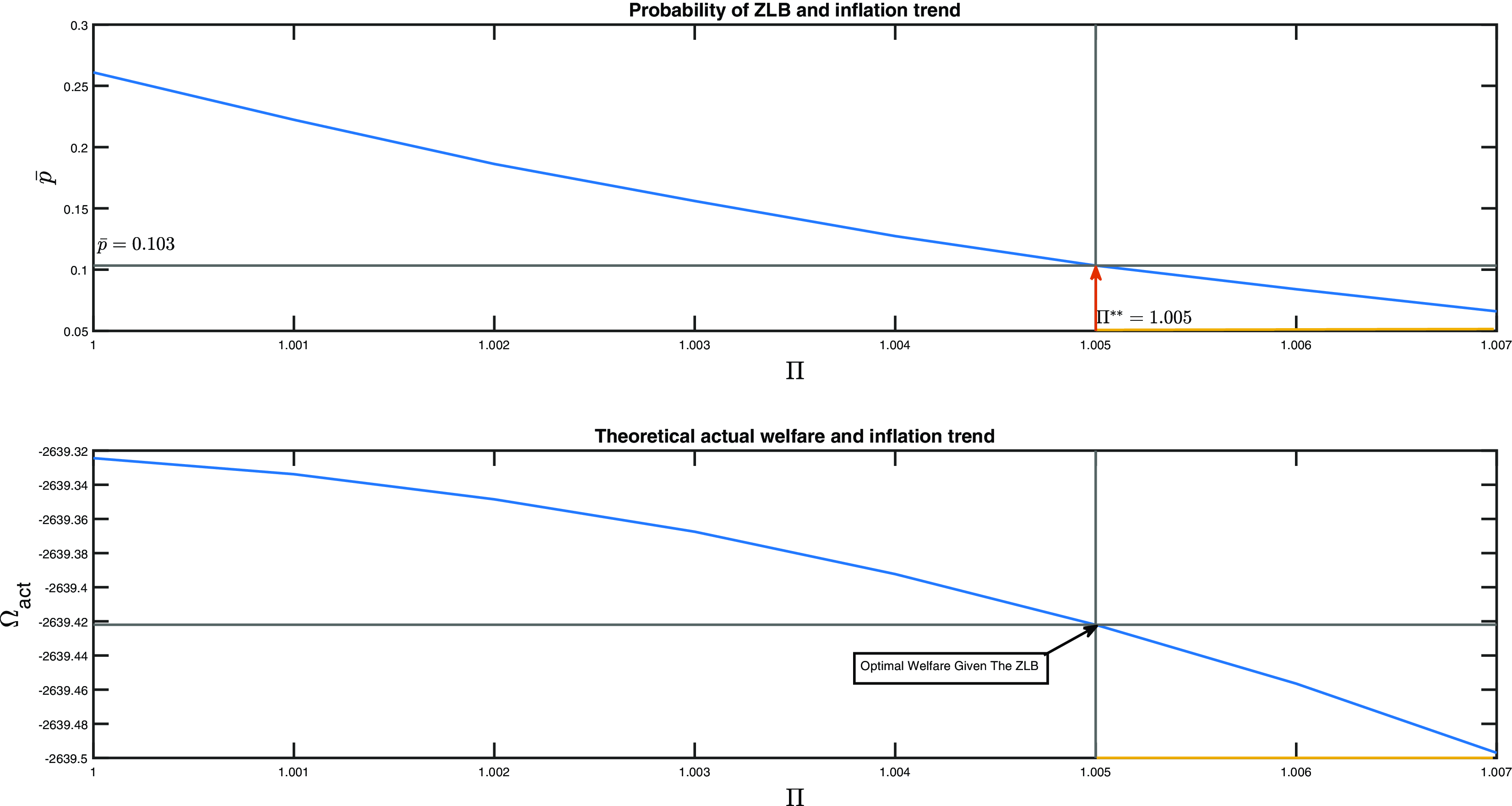
Figure 3. Figure illustrates the pick of optimal trend inflation from the set of steady-state inflation satisfying the ZLB constraint.
6.2 Stage 1: Imposing the ZLB and choice of $\Pi ^*$
and
$w_r$
$\Pi ^*$
and
$w_r$


In this section, we impose the ZLB constraint (26) where the optimal inflation target is chosen to maximize the welfare for each value of $w_r$
as explained in the previous section.
$w_r$
as explained in the previous section.
In order to examine the model’s behavior under the binding ZLB constraint, we set the value of $\bar{p}_{zlb} = 0.05$
quarterly. Other values of
$\bar{p}_{zlb} = 0.05$
quarterly. Other values of $\bar{p}_{zlb}$
will be examined later. Fig. 4 shows the outcome for some variables under the binding ZLB constraint. The first plot of Fig. 4 shows the minimum values of steady-state inflation rate,
$\bar{p}_{zlb}$
will be examined later. Fig. 4 shows the outcome for some variables under the binding ZLB constraint. The first plot of Fig. 4 shows the minimum values of steady-state inflation rate, $\Pi ^*$
, which satisfies (25) in Stage 2 with equality. As we argued above, any value of
$\Pi ^*$
, which satisfies (25) in Stage 2 with equality. As we argued above, any value of $\Pi$
which is larger than
$\Pi$
which is larger than $\Pi ^*$
satisfies the ZLB constraint, but since welfare is a decreasing function of the inflation target values, the central bank will set the lowest inflation target satisfying the ZLB. In addition, with a higher level of weight attached on the variability of the nominal interest rate, the central bank is less aggressive in conducting its monetary policy in term of stabilizing the price; that is, we see a fall in feedback rule parameter on inflation. Finally, the equilibrium is represented by the red dotted point and is documented in Table 3. Under the ZLB constraint, the optimal weight imposed on the penalty term of ZLB mandate is relatively high at
$\Pi ^*$
satisfies the ZLB constraint, but since welfare is a decreasing function of the inflation target values, the central bank will set the lowest inflation target satisfying the ZLB. In addition, with a higher level of weight attached on the variability of the nominal interest rate, the central bank is less aggressive in conducting its monetary policy in term of stabilizing the price; that is, we see a fall in feedback rule parameter on inflation. Finally, the equilibrium is represented by the red dotted point and is documented in Table 3. Under the ZLB constraint, the optimal weight imposed on the penalty term of ZLB mandate is relatively high at $w^*_r = 8$
.Footnote
20
$w^*_r = 8$
.Footnote
20
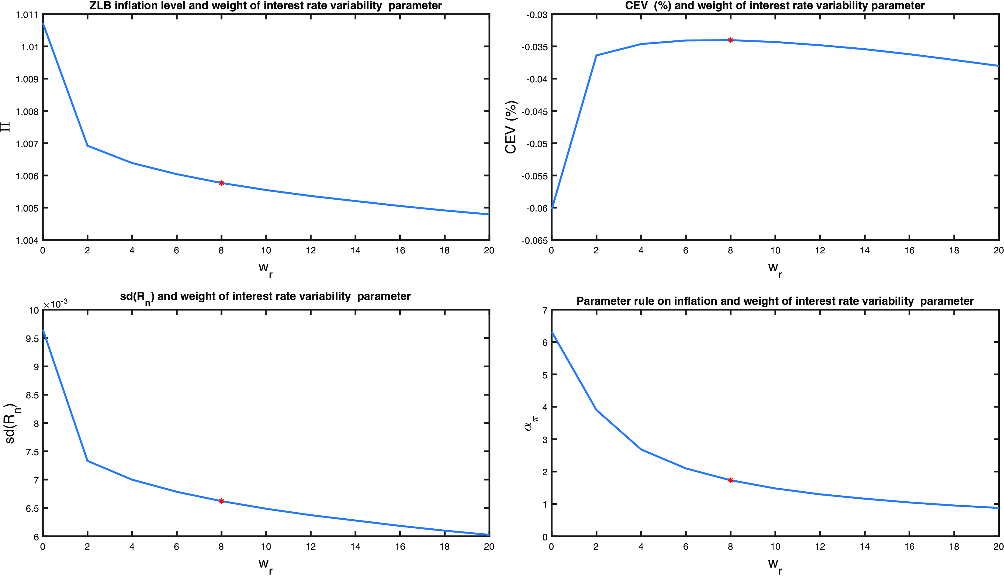
Figure 4. ZLB mandate with probability of the nominal interest rate hitting the ZLB constraint at 5%.
Table 3. Welfare stabilization from optimized rules compared with the estimated rule

Given the quarterly probability of hitting the ZLB at 1% (once quarter every 25 years), the optimal steady-state net inflation rate is then 3.7% annually. However, if we relax the ZLB constraint to an allowed probability of hitting the bound of 5%, the optimal steady-state net annual inflation is roughly 2.4%, a rate very close to the 2% inflation target of the Fed and other central banks. We also examine a probability 9.6% which is calibrated for sample data of the nominal interest rate used in the estimation exercise; we find for this probability a corresponding optimal inflation target of 1.6%. This optimal inflation rate is comparable to CGW who find that the optimal net annual inflation rate is around 1.5% in their benchmark model given their calibration of the unconditional probability of hitting the ZLB at 5% based on the post World War II (up to 2012) US experience.
The upper-right subplot in Fig. 4 expresses the behavior of the welfare gain given different values of the weight $w_r$
. Our choice of the quadratic penalty function on the policy rate, that is, the penalty on the volatility of the policy rate, results in a opening-down parabola shape, which gives us the exact value of
$w_r$
. Our choice of the quadratic penalty function on the policy rate, that is, the penalty on the volatility of the policy rate, results in a opening-down parabola shape, which gives us the exact value of $w^*_r$
where the associating optimal penalty function leads to a maximum social actual welfare. Similarly, the lower-right subplot gives us the optimal reaction of the central bank to the variation of inflation, that is, optimal feedback parameter on inflation in the Taylor rule, at the optimal
$w^*_r$
where the associating optimal penalty function leads to a maximum social actual welfare. Similarly, the lower-right subplot gives us the optimal reaction of the central bank to the variation of inflation, that is, optimal feedback parameter on inflation in the Taylor rule, at the optimal $w_r$
. Finally, the lower-left subplot indicates the level of the policy rate’s volatility at
$w_r$
. Finally, the lower-left subplot indicates the level of the policy rate’s volatility at $w^*_r$
.
$w^*_r$
.
6.3 Welfare gains from optimization and costs of the ZLB
In Table 3, we now assess the stabilization gains from optimized rules compared with the Ramsey policy using the household intertemporal welfare as the welfare criterion. By considering rules with and without the ZLB constraint its cost can also be quantified. We use the outcome of Ramsey optimum with zero net inflation and no ZLB constraint as the benchmark against which other regimes are measured. The subtables (A)–(E) focus on separate issues: in (A) the nominal interest rate rule is a component of the non-optimal estimated model and the welfare cost of this nonoptimality and that of the business cycle and is examined relative to a benchmark. In (B) this benchmark, the Ramsey optimum is reported along with the optimized rule at Stage 2 of the delegation game in the absence of a ZLB constraint and therefore no nominal interest rate penalty. In (C), the full equilibrium of the ZLB delegation game with a quadratic interest rate penalty function is reported. In (D), we compare this equilibrium with one where the quadratic penalty is replaced with the alternative asymmetric penalty as set out in Subsection 5.1. In (E), we restrict the mandate and interest rate setting rule ones with price-level targeting. Full details are as follows.
Subtable (A): Steady State Estimated Model. We first examine the steady-state welfare cost of the estimated model by setting the value of all the estimated shocks is equal to zero. The business cycle cost is relatively significant in our NK framework with a utility function that has habit and labor supply (see subtable No business cycle of Table 3).Footnote
21
Comparing the welfare outcome in the absence of shocks and with zero net inflation ( $\Pi = 1.0$
), we see that our benchmark estimated rule without the business cycle results in a welfare gain of 0.456 CEV% (= (A1)–(A4)), or equivalently the welfare cost of business cycle is 0.456% CEV with zero net inflation. This is a much higher cost of the business cycle that found in Lucas (Reference Lucas1987) and (Reference Lucas2003).Footnote
22
$\Pi = 1.0$
), we see that our benchmark estimated rule without the business cycle results in a welfare gain of 0.456 CEV% (= (A1)–(A4)), or equivalently the welfare cost of business cycle is 0.456% CEV with zero net inflation. This is a much higher cost of the business cycle that found in Lucas (Reference Lucas1987) and (Reference Lucas2003).Footnote
22
Subtable (A): Regimes of the Estimated Model. Given the estimated monetary policy shock of 0.33% (equals to the level value of 0.0033 in the Table 3) quarterly, welfare cost of the estimated inflation trend of 0.87% (3.5% annually) is approximately a 0.041% (= (A4)–(A5)) permanent reduction in consumption per quarter.Footnote
23
Note that, in this exercise, we only compare the welfare cost of inflation levels between $\Pi = 1$
and
$\Pi = 1$
and $\Pi = 1.0087$
when there is a presence of monetary policy shock equaling to 0.33% for both inflation levels.
$\Pi = 1.0087$
when there is a presence of monetary policy shock equaling to 0.33% for both inflation levels.
However, the higher empirical inflation trend results in a smaller probability of the nominal interest hitting the ZLB, that is, a zero steady-state inflation results in a per quarter probability of the ZLB incidence at 0.282 (approx 28 quarters in every 25 years), while a 3.5% of inflation trend induces a probability to 0.06 (or 6 quarters in every 25 years).
Sub-table (B): Optimized simple rule (OSR) without the ZLB constraint. Putting $w_r =0$
for these results, there is a significant welfare gain of the optimized rule compared to the estimated rule with the same steady-state inflation; that is, given a zero steady-state inflation welfare increases by 0.037 CEV% (= (B3)–(A3)). Moreover, the frequency of the nominal interest rate hitting the ZLB under optimized rule is close to that under the estimated one (0.30 to 0.28). There are two opposite impacts of these rules on the probability of the nominal interest rate hitting the ZLB. First, the optimized rule induces a lower volatility of the model compared to the estimated one, which makes the nominal interest rate also become less volatile (hence a smaller standard deviation). Second, it is the optimal value of the smoothing parameter
$w_r =0$
for these results, there is a significant welfare gain of the optimized rule compared to the estimated rule with the same steady-state inflation; that is, given a zero steady-state inflation welfare increases by 0.037 CEV% (= (B3)–(A3)). Moreover, the frequency of the nominal interest rate hitting the ZLB under optimized rule is close to that under the estimated one (0.30 to 0.28). There are two opposite impacts of these rules on the probability of the nominal interest rate hitting the ZLB. First, the optimized rule induces a lower volatility of the model compared to the estimated one, which makes the nominal interest rate also become less volatile (hence a smaller standard deviation). Second, it is the optimal value of the smoothing parameter $\rho _r$
, for example, under the estimated rule
$\rho _r$
, for example, under the estimated rule $\rho _r = 0.73$
which is much higher than that under the optimized rule (
$\rho _r = 0.73$
which is much higher than that under the optimized rule ( $\rho _r = 0.0$
). Hence, the higher the
$\rho _r = 0.0$
). Hence, the higher the $\rho _r$
, the less volatile the nominal interest rate is. As a result, probability of the nominal interest rate hitting the ZLB becomes almost equal.
$\rho _r$
, the less volatile the nominal interest rate is. As a result, probability of the nominal interest rate hitting the ZLB becomes almost equal.
We also examine the performance of the original Taylor rule with its parameters calibrated from Taylor (Reference Taylor1993). Overall, there is a large welfare cost associated with the original Taylor rule of approximately 2.23–2.677 CEV% for the same target inflation rate and a very high probability of the nominal interest rate hitting the ZLB. This indicates that the inertia term on nominal interest rate, which is absent in the original Taylor rule, plays a crucial role in stabilizing the economy and lowering the possibility of the ZLB episode.
Finally in subtable (B), we compare outcomes with the Ramsey optimal policy (used as our benchmark about which the CEV is measured). As in Schmitt-Grohe and Uribe (Reference Schmitt-Grohe and Uribe2007), we find the optimized simple rule (OSR) with $\Pi =1$
but with no ZLB considerations, closely mimics this equilibrium.
$\Pi =1$
but with no ZLB considerations, closely mimics this equilibrium.
Subtable (C): Optimized simple rule (OSR) with the ZLB constraint. To examine the welfare cost of the ZLB constraint, we now consider how changes in the frequency of nominal interest rate hitting the ZLB affect welfare by examining different values of $\bar{p}_{zlb}$
. We consider three different levels of
$\bar{p}_{zlb}$
. We consider three different levels of $\bar{p}_{zlb}$
: 0.01 (one quarter every 25 years), 0.05 (five quarters every 25 years), and 0.096 (approx 10 quarters every 25 years). The 0.05 corresponds to the post-WWII experience of the USA used the calibration of CGW (up to 2012) while the latter considers the calibrated value of the data sample for estimation exercise which fully takes in account the ZLB period during the financial crisis and aftermath. Proceeding from the most to the least frequent of ZLB episodes, we then see the CEV cost rising from 0.024% ((C(3))) to 0.061% ((C(1))).
$\bar{p}_{zlb}$
: 0.01 (one quarter every 25 years), 0.05 (five quarters every 25 years), and 0.096 (approx 10 quarters every 25 years). The 0.05 corresponds to the post-WWII experience of the USA used the calibration of CGW (up to 2012) while the latter considers the calibrated value of the data sample for estimation exercise which fully takes in account the ZLB period during the financial crisis and aftermath. Proceeding from the most to the least frequent of ZLB episodes, we then see the CEV cost rising from 0.024% ((C(3))) to 0.061% ((C(1))).
Our framework results in this welfare loss of ZLB episodes from two sources. First, the optimal steady-state inflation rate rises which, as discussed in Section 2.1, directly generates a welfare loss in the New Keynesian model through a higher price and wage dispersion. Second, the optimal mandate (the optimal determination of the penalty term in the delegated mandate, $w^*_r$
) generates a suboptimal result from the social welfare point by constraining the use of the nominal interest rate for stabilization. It is worth noting that as the constraint becomes tighter, the optimized simple rule converges to a Taylor-type rule with a very high persistence.
$w^*_r$
) generates a suboptimal result from the social welfare point by constraining the use of the nominal interest rate for stabilization. It is worth noting that as the constraint becomes tighter, the optimized simple rule converges to a Taylor-type rule with a very high persistence.
Subtable (D): Optimized simple rule (OSR) with an asymmetric ZLB constraint. We next investigate the framework under an asymmetric formation of the ZLB mandate in the spirit of Den Haan and Wind (Reference Den Haan and Wind2012), which only penalizes the zero net interest rate in an asymmetric fashion. This type of central bank’s objective function implies that there is asymmetry under various economic structures which is fully taken into account by the central bank in conducting it monetary policy. The results in Table 3 are very similar in the symmetric and asymmetric cases suggesting that our ZLB mandate result is robust across these different forms of the ZLB mandate.
Subtable (E): Optimized price level rule. We next consider a special case of the Taylor-type simple rule (29):
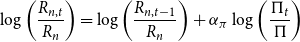 \begin{equation} \log \left( \frac{R_{n,t}}{R_n}\right)=\log \left( \frac{R_{n,t-1}}{R_n}\right) +\alpha _\pi \log \left(\frac{\Pi _{t}}{\Pi }\right) \end{equation}
Integrating the rule above gives:
 \begin{equation} \log \left( \frac{R_{n,t}}{R_n}\right)=\alpha _\pi \log \left(\frac{P_{t}}{\bar{P}_t}\right) \end{equation}
which is a price level rule with the trend price level given by $\frac{\bar{P}_t}{\bar{P}_{t-1}}=\Pi$
.
$\frac{\bar{P}_t}{\bar{P}_{t-1}}=\Pi$
.
Giannoni (Reference Giannoni2014) argues that such simple price-level rule, comparing to the simple rule that responds to inflation, delivers superior results in several aspects of optimal monetary policy in the context of a NK model. First, price-level stabilization delivers outcomes that are closest to optimal. Second, such a policy has a robustness feature that delivers desirable outcomes even in the face of key types of model misspecification. Finally, price-level stabilization is more likely to result in a unique bounded equilibrium. Our results add a further advantage: the price-level rule closely mimics the general optimized rule with potential output feedbacks so price-level targeting helps to escape the ZLB. The intuition for the benefits of price targeting is as follows: faced with of an unexpected temporary rise in inflation price-level stabilization commits the Central Bank to bring inflation below the target in subsequent periods. In contrast, with inflation targeting, the drift in the price level is accepted.
Subtable E of the Table 3 represents the results of our mandate framework when the central bank is committed to price-level targeting rule. Overall, the price-level targeting rule replicates the mandate equilibrium. However, without a small trade-off between inflation and output activities, there is a higher welfare loss under the price-level targeting rule compared to the optimized simple rule.
6.4 A case for a 4% annual trend inflation target
In light of the recent consistent effective lower bound to central bank interest rates, the literature has also suggested that it is desirable to raise the inflation target to 4% to combat the ZLB on nominal interest rates (see for example Ball (Reference Ball2013)). In this section, we examines the impact of a 4% annual inflation trend scenario on the probability of the nominal interest rate hitting the ZLB in via our framework.
Results (C) and (D) from Table 3 suggest that if the gross quarterly inflation target is set at $\Pi ^*$
ranging from
$\Pi ^*$
ranging from $1.0093$
to
$1.0093$
to $1.00993$
which is equivalent to the net inflation ranging from
$1.00993$
which is equivalent to the net inflation ranging from $3.73$
% to
$3.73$
% to $3.77$
% annually, the ZLB episode would happen at a very low frequency of 1 quarters every 25 years. A 4% (subtable (F) from Table 3) target would then bring the frequency down even further to
$3.77$
% annually, the ZLB episode would happen at a very low frequency of 1 quarters every 25 years. A 4% (subtable (F) from Table 3) target would then bring the frequency down even further to $0.007$
if this is indeed what the policymaker aims for. Ascari and Ropele (Reference Ascari and Ropele2007) suggest that a case of 4% inflation trend would indeed give a leeway for the central bank under the effective lower bound on nominal rates episode, but will also significantly narrows the determinacy region for monetary policy rules. But this is not a concern for our optimized rules as parameters are chosen to lie within the determinacy region.
$0.007$
if this is indeed what the policymaker aims for. Ascari and Ropele (Reference Ascari and Ropele2007) suggest that a case of 4% inflation trend would indeed give a leeway for the central bank under the effective lower bound on nominal rates episode, but will also significantly narrows the determinacy region for monetary policy rules. But this is not a concern for our optimized rules as parameters are chosen to lie within the determinacy region.
7. Quadratic loss function mandates: Numerical results
We now turn to simple quadratic loss function mandates designed to increase transparency in the conduct of monetary policy. In the four mandates below, the particular loss function is matched with a simple rule with the same targets. Thus, the transparency of the loss function is reinforced with that of the interest rate rule. We first set out the details of the mandates followed by numerical results. A final subsection compares and discusses these results across mandates. The reader should recall that the probability 9.6% of hitting the ZLB is calibrated for sample data of the nominal interest rate used in the estimation exercise and should note that the baseline welfare loss about which the CEV calculation is that from the optimized simple rule (OSR) in Table 3 for the Case (B) where no ZLB is imposed and the target steady-state inflation is set at $\Pi =1$
.
$\Pi =1$
.
7.1 Mandates I–IV
Our mandate I is expressed in terms of the growth of output $\frac{Y_t}{Y_{t-1}}$
and gross inflation
$\frac{Y_t}{Y_{t-1}}$
and gross inflation $\Pi _t$
relative to their steady states. The delegated mandate I now consists of:
$\Pi _t$
relative to their steady states. The delegated mandate I now consists of:
 \begin{eqnarray} \Omega _t^{mod} \equiv - \mathbb{E}_t\left [ \sum _{\tau =0}^\infty \beta ^{\tau } \left(\left(\Pi _{t+\tau } - \Pi \right)^2 + w_{dy} \left(\frac{Y_{t+\tau }}{Y_{t+\tau -1}} - (1+g) \right)^2 + w_r \left(R_{n,t+\tau } - R_n \right)^2 \right) \right ] \end{eqnarray}
with a corresponding simple rule:
 \begin{equation} \log \left( \frac{R_{n,t}}{R_n}\right)=\rho _r \log \left( \frac{R_{n,t-1}}{R_n}\right) +\alpha _\pi \log \left(\frac{\Pi _{t}}{\Pi }\right) + \alpha _{dy} \log \left(\frac{Y_t}{Y_{t-1}}\right) \end{equation}
Our next mandate II is a special form of the price-level rule corresponding to strict inflation targeting mandate:
 \begin{eqnarray} \Omega _t^{mod} \equiv - \mathbb{E}_t\left [ \sum _{\tau =0}^\infty \beta ^{\tau } \left(\left(\Pi _{t+\tau } - \Pi \right)^2 + w_r \left(R_{n,t+\tau } - R_n \right)^2 \right) \right ] \end{eqnarray}
with a corresponding simple rule
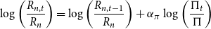 \begin{equation} \log \left( \frac{R_{n,t}}{R_n}\right)= \log \left( \frac{R_{n,t-1}}{R_n}\right) +\alpha _\pi \log \left(\frac{\Pi _{t}}{\Pi }\right) \end{equation}
Mandate III is expressed in terms of real wage growth $\frac{W_t}{W_{t-1}}$
and gross inflation
$\frac{W_t}{W_{t-1}}$
and gross inflation $\Pi _t$
relative to their steady states. The delegated mandate now consists of:
$\Pi _t$
relative to their steady states. The delegated mandate now consists of:
 \begin{align} \Omega _t^{mod} \equiv - \mathbb{E}_t\left [ \sum _{\tau =0}^\infty \beta ^{\tau } \left(\left(\Pi _{t+\tau } - \Pi \right)^2 + w_{dw} \left(\frac{W_{t+\tau }}{W_{t+\tau -1}} -(1+g) \right)^2 + w_r \left(R_{n,t+\tau } - R_n \right)^2 \right) \right ] \end{align}
with a corresponding simple rule
 \begin{equation} \log \left( \frac{R_{n,t}}{R_n}\right)=\rho _r \log \left( \frac{R_{n,t-1}}{R_n}\right) +\alpha _\pi \log \left(\frac{\Pi _{t}}{\Pi }\right) + \alpha _{dw} \log \left(\frac{W_t}{W_{t-1}}\right) \end{equation}
Our final transparent delegated mandate IV is expressed in terms of employment growth $\frac{H_t^d}{H_{t-1}^d}$
and gross inflation
$\frac{H_t^d}{H_{t-1}^d}$
and gross inflation $\Pi _t$
relative to their steady states. The delegated mandate now consists of:
$\Pi _t$
relative to their steady states. The delegated mandate now consists of:
 \begin{eqnarray} \Omega _t^{mod} \equiv - \mathbb{E}_t\left [ \sum _{\tau =0}^\infty \beta ^{\tau } \left(\left(\Pi _{t+\tau } - \Pi \right)^2 + w_{dh} \left(\frac{H^d_{t+\tau }}{H^d_{t+\tau -1}} -1 \right)^2 + w_r \left(R_{n,t+\tau } - R_n \right)^2 \right) \right ] \end{eqnarray}
Corresponding simple rule:
 \begin{equation} \log \left( \frac{R_{n,t}}{R_n}\right)=\rho _r \log \left( \frac{R_{n,t-1}}{R_n}\right) +\alpha _\pi \log \left(\frac{\Pi _{t}}{\Pi }\right) + \alpha _{dh} \log \left(\frac{H^d_t}{H^d_{t-1}}\right) \end{equation}
7.2 Numerical results for four mandates
Table 4 set out the numerical results for our four quadratic mandates. Again we set out the optimized rule for the central bank that, for each mandate, uses a quadratic loss function set out in Section 7.1 plus a interest rate penalty term. For each ZLB probability (the empirical $\bar{p}_{zlb}=0.096$
and the policy choices
$\bar{p}_{zlb}=0.096$
and the policy choices $\bar{p}_{zlb}=0.05, 0.01$
), we report the welfare-optimal combination of the gross infaltion target
$\bar{p}_{zlb}=0.05, 0.01$
), we report the welfare-optimal combination of the gross infaltion target $\Pi$
and penalty weights for each mandate using the actual household welfare as the criterion. The welfare-optimal mandate is then described by the choice of weights
$\Pi$
and penalty weights for each mandate using the actual household welfare as the criterion. The welfare-optimal mandate is then described by the choice of weights $(\Pi ^*, w_r^*, w_{dy}^*)$
for mandate I,
$(\Pi ^*, w_r^*, w_{dy}^*)$
for mandate I, $(\Pi ^*, w_r^*)$
for mandate II,
$(\Pi ^*, w_r^*)$
for mandate II, $(\Pi ^*, w_r^*, w_{dw}^*)$
for mandate III and
$(\Pi ^*, w_r^*, w_{dw}^*)$
for mandate III and $(\Pi ^*, w_r^*, w_{dh}^*)$
for mandate IV. This choice depends on the tightness of the ZLB constraint,
$(\Pi ^*, w_r^*, w_{dh}^*)$
for mandate IV. This choice depends on the tightness of the ZLB constraint, $\bar{p}_{zlb}$
for each case. In the table below, we report this welfare-optimal equilibrium for each mandate along with the actual welfare. The latter is also expressed in consumption-equivalen terms relative to the Ramsey optimum set out in Table 3. Full details of choosing the grids on the weights are presented in the appendices (Tables 3–6).
$\bar{p}_{zlb}$
for each case. In the table below, we report this welfare-optimal equilibrium for each mandate along with the actual welfare. The latter is also expressed in consumption-equivalen terms relative to the Ramsey optimum set out in Table 3. Full details of choosing the grids on the weights are presented in the appendices (Tables 3–6).
Table 4. Results for quadratic mandates
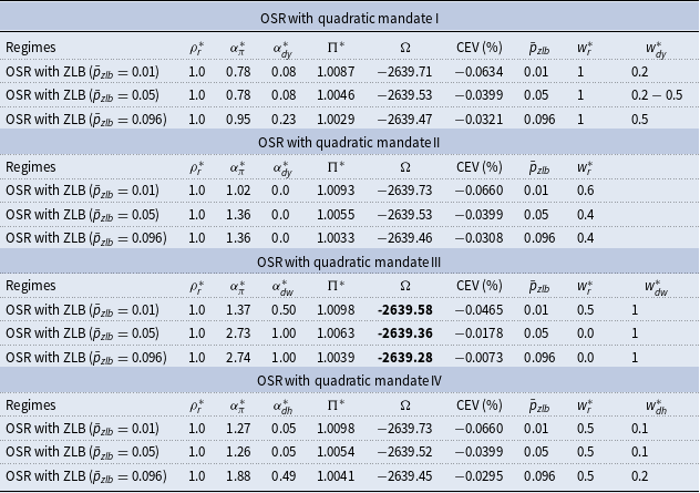
For these optimal mandates, we find that the weights attached to real economic activities based on a normalized unit quarterly inflation and quarterly rates of change of real variables are in the range 0.2–1.0. So we find some support for a dual mandate, but less than DKLN who find that simple loss functions should feature a weights of almost 3 for output growth.
The source of these differences in our framework lies in the model summarized in Section 3.6, the presence of the ZLB constraint and the coupling of the optimized appropriate interest rate rule with the loss function mandate. Considering the first of these, the Kimball aggregator in the original SW model (but not included in our set-up for reasons discussed in Section 3.6) adds a real rigidity to the model and providing a reason for designing policy to respond to the effects of shock on real variables such as output growth. The trend-inflation effect that is removed in Smets and Wouters (Reference Smets and Wouters2007), but present in our set-up, makes price and wage dispersion respond up to first order to shocks to price and wage inflation creating a reason for policy to react more to changes in the inflation rate for both the instrument rule and the comparable mandate. Another source of the difference is the nature of the delegation game. Whereas DKLN studies a Ramsey problem with the simple loss function as parsimonious approximations to social welfare, our paper investigates a simple interest-rate rule regime which matches the delegated a loss function. This limits the ability of the nominal interest rate to respond to the to any macroeconomic aggregate compared with the complex implied Ramsey rule and shifts the response of the optimized rule and the comparable mandate toward the inflation target.
However, for the best mandate III, which involve real wage growth targeting, the optimized interest rate rule responds strongly to this component. In doing so, it also reduces nominal wage dispersion resulting in a further welfare benefit.Footnote
24
The associated optimal mandate then has a weight on wage growth close to that on inflation, that is, $w_{dw}^*=1$
.
$w_{dw}^*=1$
.
7.3 General discussion
We have examined several forms of transparent loss function mandates that impose the ZLB constraint by penalizing the volatility of nominal interest rate. The results are striking in several respects. First, from the actual (representative household) welfare criterion, the integrated-ZLB conventional inflation-output optimal mandate I results in the highest welfare loss, while the nominal price and wage inflation targeting mandate IV lead to the lowest. The consumption equivalent differences are quite small and of the order 0.01%. But for all optimal mandates, there is a substantial welfare stabilization gain of the order of 0.1% compared with the outcome of the estimated rule. Generally in our NK model with labor supply and habit in the utility function and with price and wage stickiness both the welfare costs of the business cycle and the potential gains from stabilization policy are substantially greater than those found by Lucas (Reference Lucas2003) and in the RBC model without such distortions.
Second, in the quadratic mandates, the optimal weights attached to real economic activities (i.e., output or labor demand) are relatively small compared with the weight attached to quarterly price inflation. Only for mandate III targeting directly both nominal price and real wage growth do we find that the relative optimal weights attached to these targets are close to unity. This result contrasts with the strong support for the dual mandate found by DKLN where with a mandate with real activity output growth a weight of almost 3 is reported. The source of this difference has been discussed in Subsection 7.2.
Third, the associated optimized simple rules all converge to a price-level targeting rule, or at least to an interest-rate rule with the smoothing component on the nominal interest rate close to unity. Overall, the central bank reacts positively to output and labor demand, so a looser monetary policy corrects for a decline in these real economic variables. However, because the optimized weights in the loss function are relatively small, these real economic activity components also carry a small weight in the optimized simple rules.
Fourth, the formation of the optimal mandates has a little impact on the optimal steady-state inflation level. Overall, the optimal steady-state inflation does not vary across different formations of the mandate and the tightness level of the ZLB (the allowed probability of the nominal interest rate hitting the ZLB) is the main driving force on the optimal steady-state inflation. The allowed highest quarterly probability of 9.6% (approx 10 quarters every 25 years) corresponds to the data sample of the estimation exercise. We find that the optimal level of inflation trend rate is close to 1.2%, which is close to the result produced by CGW who calibrated the quarterly probability of 5% (approx 5 quarters every 25 years) which they note is consistent with the historical experience of the ZLB frequency for the USA from 1945 to 2012. In addition, with the calibrated quarterly probability of 5% in our study, we find the optimal inflation trend rate is close to the typical common-known 2% of most prominent central banks. There are two possible reasons for this discrepancy: first, our model is estimated by Bayesian methods with an empirical inflation trend and could claim to be more empirical; second, our choice of welfare function to design the mandate avoids any quadratic steady-state small-distortions approximation. We use a second-order perturbation approach that only assumes the variance of shocks are small which is confirmed in the estimation. We suspect that the first of these two reasons is the more important. Overall, the debate of optimal inflation target hinges entirely on the allowed probability of hitting ZLB.
8. Conclusions
Our paper has presented a general framework for monetary policy delegated to an instrument-independent but goal-dependent central bank. The latter is mandated to optimize a particular form of interest rate rule with a steady-state inflation target. The goal mandate includes a penalty on the interest rate variance chosen to be welfare-optimal given the constraint of hitting the ZLB with a particular frequency. Different goal mandates are considered all associated with Taylor-type simple rules with the same target variables.Footnote 25
So is there support for dual mandate from our study as highlighted in DKLN? We too find some support for a dual mandate as well, but less so in two respects: first the mandate weights in real activity are significantly less than unity except when the loss function is expressed in terms of real wage growth. Second, the fact that a pure inflation welfare target coupled with a price-level rule mimics all other mandates very closely.
Regarding the optimal inflation target, our paper supports the view that raising the inflation target above the standard 2% per year to 4% is a feasible welfare-enhancing mandate for the central banks to deal effectively with the ZLB, but only if the required quarterly frequency of violating the constraint falls to well under 1%. The price-level form of the optimized rule avoids the indeterminacy problem highlighted by proponents of the 2% target.
Future work will explore a number of directions: first, by our choice of Dixit-Stiglitz rather than Kimball aggregators, for reasons discussed in Section 3.6, we have removed a real friction. A recent study by Galí (Reference Galí2018) suggests that an alternative real friction in the form of labor market hysteresis has important consequences for the conduct of monetary policy. This would replace the Calvo-wage setting with a labor market in which the optimized nominal wage is set by trade-unions such that in expectation a weighted average of employment equals an exogenous target over the period for which the wage remains effective. Another possible development of our framework, following CGW, could examine state-dependent wage and price contracts with endogenous durations. An interesting question is whether our results carry over to the open economy. In the open economy the exchange rate provides a further expenditure switching channel for interest rate policy which would potentially change our results. In a sticky-price environment the pricing paradigms (local currency pricing versus producer currency pricing) is another important consideration for optimized rules with a ZLB which is studied in Mirfatah et al. (Reference Mirfatah, Gabriel and Levine2021), but with no consideration of simple mandates. Finally, mandate framework can be examined in a behavioral NK model that relaxes the rational expectations assumption in different ways.Footnote 26
Supplementary material
The supplementary material for this article can be found at https://doi.org/10.1017/S136510052300024X.


 Open access