


1. Introduction
Fama and French’s (Reference Fama and French1992, Reference Fama and French1993, Reference Fama and French1996, Reference Fama and French1998, Reference Fama and French2015, Reference Fama and French2016) seminal contributions shed skeptical light on the empirical performance of the Capital Asset Pricing Model (CAPM) of Sharpe (1964) and Lintner (Reference Lintner1965). The subsequent search for a better asset return model has been a hot pursuit for many financial economists (Fama and French (Reference Fama and French1993, Reference Fama and French1995, Reference Fama and French1996, Reference Fama and French1998, Reference Fama and French2006b, Reference Fama and French2008, Reference Fama and French2015; Hou et al. (2014)). Financial economists engage in the relentless debate over whether dramatic movements in market valuation such as the Global Financial Crisis reflect a “rational” fair-value price correction or a lack of compensation for risk. The debate has left many financial economists at a time-worn impasse (Fama and French, Reference Fama and French2004). Empiricists continue to discover new asset anomalies (e.g., Titman et al. (2004); Fama and French (Reference Fama and French2006b, Reference Fama and French2008); Cooper et al. (Reference Cooper, Gulen and Schill2008); Li et al. (Reference Li, Livdan and Zhang2009); Novy-Marx (Reference Novy-Marx2013)).
Kozak et al. (Reference Kozak, Nagel and Santosh2017; Reference Kozak, Nagel and Santosh2018) recent studies show that many recent empirical horse races cannot draw a distinction between both rational and behavioral theories of average return evolution. Kozak et al. (Reference Kozak, Nagel and Santosh2018) report that a factor model with a small number of statistical principal-components (PCs) performs as well as the prior factor models (e.g. Fama and French (Reference Fama and French1993); Hou et al. (Reference Hou, Xue and Zhang2015); Fama and French (Reference Fama and French2015); Novy-Marx and Velikov (Reference Novy-Marx and Velikov2016); Barillas and Shanken (Reference Barillas and Shanken2018)). For typical portfolios, these few factors dominate the covariance matrix of returns. In the absence of near-arbitrage investment opportunities, these factor models include only a few dominant factors, which can be fundamental characteristics such as size and book-to-market or purely statistical PCs. Because these models exhibit few conceptual links to investor beliefs and preferences, the q-theoretic factor models are as much “behavioral models” as the models are “rational models” (cf. Berk et al. (Reference Berk, Green and Naik1999); Johnson (Reference Johnson2002); Gomes et al. (Reference Gomes, Kogan and Zhang2003); Liu et al. (2011); Liu and Zhang (Reference Liu and Zhang2008); Lin and Zhang (Reference Lin and Zhang2013); Liu and Zhang (Reference Liu and Zhang2014)). In a similar vein, the prior tests of characteristics-versus- covariances inform us little of whether and how behavioral barriers such as investor sentiment and overconfidence affect asset returns (e.g., Daniel and Titman (Reference Daniel and Titman1997); Brennan et al. (Reference Brennan, Chordia and Subrahmanyam1998); Davis et al. (Reference Davis, Fama and French2000); Stambaugh and Yuan (2017)). Overall, it seems futile to implement these horseraces to assess the complex convolution of both investor sentiment and rationality in most asset return tests.
In the current study, we carry out an alternative approach to tackling this important issue in finance. We first extract all dynamic conditional factor premiums from the Fama and French (Reference Fama and French2015) model and then find that most anomalies disappear after one accounts for time variation in these premiums. Granger-causality tests suggest new mutual causation between dynamic conditional alpha spreads and macroeconomic innovations. This mutual causation therefore serves as a core qualifying condition for factor selection with sound economic motivation. In the current study, our economic insight is an incremental step toward drawing a distinction between both rational risk and behavioral models in response to Kozak et al. (Reference Kozak, Nagel and Santosh2017; Reference Kozak, Nagel and Santosh2018). To the extent that macroeconomic surprises manifest in the form of dynamic conditional alphas, this causation can reveal the marginal investor’s fundamental news and expectations about the cross-section of average returns. Hence, our evidence contributes to macroeconomic asset return prediction.
Kozak et al. (Reference Kozak, Nagel and Santosh2018) point out that the presence of arbitrageurs will connect the covariance structure to the cross-section of average returns. Insofar as this cross-section at least partially reflects investor sentiments such as overconfidence, salience of recent experience, and other cognitive biases, behavioral mispricing factors can help price assets with reasonable bounds on the Sharpe ratios. In this context, these behavioral factors load reasonable premiums to correctly price assets. However, these behavioral factors and premiums “will not necessarily covary with aggregate macroeconomic risks , as the [fundamental factors] would…” (cf. Kozak et al. (Reference Kozak, Nagel and Santosh2017, Reference Kozak, Nagel and Santosh2018); Daniel et al. (Reference Daniel, Hirshleifer, Sun, Daniel, Mota, Rottke and Santos2017); Daniel et al. (Reference Daniel, Hirshleifer, Sun, Daniel, Mota, Rottke and Santos2017)). In fact, Kozak et al. (Reference Kozak, Nagel and Santosh2018) suggest several alternative routes to design asset return tests that are more informative about investor beliefs, behaviors, and preferences:
“To devise tests that are more informative about investor beliefs, researchers must exploit additional predictions of a factor model that relate returns to other data such as macroeconomic variables , information on portfolio holdings, or data on investor beliefs” (cf. Kozak et al. (Reference Kozak, Nagel and Santosh2018): Section III.C first paragraph with our own bold italic emphasis).
In the current study, we pick the low-hanging fruit through an empirical analysis of mutual causation between macroeconomic innovations and dynamic conditional factor premiums. To the extent that macroeconomic innovations manifest in the form of dynamic conditional alphas and betas, the conditional moments of returns and factors convey information about the cross-section of average returns. This causation can thus serve as a core qualifying condition for valid and sound factor selection in macroeconomic asset return prediction. In particular, our evidence lends credence to the ubiquitous use of Fama and French (Reference Fama and French2015) factors that can reveal the marginal investor’s response to fundamental expectations about the cross-section of average returns. At the same time, however, our econometric tests support Fama and French’s (Reference Fama and French1996, Reference Fama and French2008, Reference Fama and French2015, Reference Fama and French2016) perennial reluctance to consider the Carhart (Reference Carhart1997) momentum factor in their factor model. We connect our dynamic conditional factor model results to recent advances in the intertemporal CAPM context (Merton (Reference Merton1973); Campbell (Reference Campbell1993); Campbell and Vuolteenaho (Reference Campbell and Vuolteenaho2004); Campbell et al. (Reference Campbell, Giglio, Polk and Turley2017)). On balance, our current study represents an incremental step toward better deciphering a distinction between the rational risk paradigm and the behavioral mispricing conjecture.
We acknowledge the fact that some recent studies replicate a broader basket of anomalies (cf. Fama and French (Reference Fama and French2016); Harvey et al (Reference Harvey, Liu and Zhu2016); Hou, et al. (Reference Hou, Xue and Zhang2017); Harvey (Reference Harvey and Liu2017); Chordia et al. (Reference Chordia, Goyal and Saretto2017)). Our primary and ultimate goal is not to compete with these prominent authors with more empirical replication. Instead, we establish new Granger causation between dynamic conditional alpha spreads and macroeconomic innovations as a core qualifying condition for fundamental factor selection in macro asset return prediction. This condition adds sound economic rigor and intuition to macroeconomic asset return prediction. So this condition contributes to our fresh insight that bilateral causation between macroeconomic surprises and dynamic conditional alpha spreads reflects the marginal investor’s fundamental news and macro expectations about the cross-section of average returns. This fresh insight can help demystify the empirical puzzle that Kozak et al. (Reference Kozak, Nagel and Santosh2018) suggest in their recent research.
Macroeconomic innovations move in tandem with dynamic conditional factor premiums that provide unique economic insights into the implicit nexus between state-dependent alphas and betas across fundamental factors. This nexus reveals rich information about the conditional factor covariance matrix in contrast to the unconditional counterpart, the latter of which omits informative restrictions across the conditional moments of both asset returns and factors from the empirical assessment of goodness-of-fit (Nagel and Singleton (Reference Nagel and Singleton2011)). Not only do dynamic conditional alpha spreads change over time, but these alpha spreads also exhibit a robust causal relation with macroeconomic surprises in a standard vector autoregressive system (Sims (1980)). Macroeconomic innovations Granger-cause most dynamic conditional alpha spreads except for momentum and partial value. Granger causation runs in a bilateral direction such that dynamic conditional alpha spreads both lead and convey material information about macro innovations (cf. our subsequent explanatory text on Section 4 and Tables 6, 7, 8 and 9).
This evidence enriches our key interpretation of the intertemporal CAPM that macroeconomic gyrations both lead and vary with the conditional expectations of terminal payoffs in the marginal investor’s intertemporal selection (Merton (Reference Merton1973); Campbell (Reference Campbell1993); Fama (Reference Fama1996); Campbell and Vuolteenaho (Reference Campbell and Vuolteenaho2004); Campbell et al. (Reference Campbell, Giglio, Polk and Turley2017)). Macro innovations manifest in the form of dynamic conditional alpha spreads that persist as abnormal returns. Therefore, mutual Granger causation between macro surprises and dynamic conditional alpha spreads becomes an informative piece of evidence that we can apply to help resolve some long prevalent asset anomalies.
With this theoretical justification of the intertemporal CAPM, we contribute to the empirical design of a workhorse asset return model by qualifying specific fundamental factors as useful and reasonable state variables. Our core qualifying condition is equivalent to mutual causation between macro surprises and alpha spreads that reflect changes in the conditional expectations of structural shifts in terminal wealth for the marginal investor. To the extent that many residual macroeconomic fluctuations lead dynamic conditional alpha spreads and vice versa, this causal relation becomes a necessary condition for valid and effective factor selection in empirical asset return research. For this pivotal purpose, sound theoretical justification of fundamental factors with respect to causal macroeconomic innovations should precede pure empirical motivation in macroeconomic asset return prediction (Harvey (Reference Harvey and Liu2017); Harvey et al. (Reference Harvey, Liu and Zhu2016)).
Our current study also contributes to the conditional multifactor model literature. It is well-known that a dynamic conditional mean-variance efficient return need not unconditionally price the static portfolios with constant weights (cf. Cochrane (Reference Cochrane2005: 140)). Specifically, if a portfolio return is on the conditional mean-variance efficient frontier, this return may or may not land on the unconditional mean-variance efficient frontier. Cochrane (Reference Cochrane2005: 168) describes this issue in a succinct statement: “Whether the [multifactor model] can be rescued by more careful treatment of conditioning information remains an empirical question”. In the current study, we attempt to fill this theoretical void by conditioning the main prediction of average returns on Fama and French (Reference Fama and French2015) factors up to each time increment. Subsequent work substantiates our economic insight that reconciles a reasonable array of anomalies within the dynamic conditional factor model.
Our unique use of fresh econometric tools serves as another empirical contribution to the asset return literature. Both the conditional specification test and recursive multivariate filter help extract dynamic conditional factor premiums that covary with macro surprises substantially over time. Conditional on the expectation of zero prior prediction error, the recursive multivariate filter updates all of the dynamic alpha-beta factor premiums up to each time increment in real-time. This important econometric innovation extends and generalizes the Fama-French multiple-regression approach and therefore can become part of the standard toolkit for subsequent asset pricing analysis. This application reconciles a baseline array of anomalies with the central theme of “dynamic” multifactor mean-variance efficiency (cf. dynamic MMVE in Fama (Reference Fama1996) and Merton (Reference Merton1973)). Further, the concomitant tests provide evidence in support of this notion. As a result, dynamic MMVE can serve as an informative benchmark for the empirical assessment of pervasive anomalies or portfolio strategies that generate persistent abnormal returns in a static context. Overall, our dynamic conditional factor model thus has key implications for equity cost estimation, risk management, fund performance evaluation, and corporate event assessment.
Applying the recursive multivariate filter adds value to the notion of dynamic multifactor mean variance efficiency (MMVE) in the intertemporal asset pricing context (cf. Merton (Reference Merton1973); Campbell (Reference Campbell1993); Fama (Reference Fama1996); Campbell and Vuolteenaho (Reference Campbell and Vuolteenaho2004); Campbell et al. (Reference Campbell, Giglio, Polk and Turley2017)). In this context, investors care about not only their terminal wealth but also state variables such as human capital, labor income, consumption, and hedging investment opportunities that covary with their terminal wealth (Fama and French (Reference Fama and French2004)). For instance, several studies suggest that inter-industry heterogeneity in both human capital and labor mobility can help explain the cross-section of average returns (Eiling (Reference Eiling2013); Donangelo (Reference Donangelo2014)). An international factor model with Epstein and Zin (Reference Epstein and Zin1989) recursive investor preferences explains the high correlation of stock market indices despite the low correlation of fundamental factors (Colacito and Croce (Reference Colacito and Croce2011)). A twin-country model can demystify both the carry trade puzzle and low correlation between exchange rate movements and cross-country differences in total consumption in the intertemporal context (Colacito and Croce (Reference Colacito and Croce2013)). Hence, the Fama and French (Reference Fama and French2015) factors serve as valid and relevant empirical hedging instruments for the marginal investor’s intertemporal selection between his or her current and future investment opportunities. Our current work suggests that the exclusion of Fama-French factors leads the econometrician to reject the null hypothesis of a correct factor model specification (Fama and French, Reference Fama and French2016). Specifically, we find mutual Granger causation between macroeconomic surprises and dynamic conditional alphas for the Fama and French (Reference Fama and French2015) fundamental factors, except for momentum and partial value. This latter falsification provides empirical justification of Fama and French’s (Reference Fama and French1993, Reference Fama and French1996, Reference Fama and French2015, Reference Fama and French2016) perennial reluctance to encompass Carhart (Reference Carhart1997) momentum as a new fundamental factor in the rational risk paradigm. All of this evidence thus bolsters our intertemporal CAPM interpretation of fundamental factors for the dynamic conditional factor model.
To the extent that macroeconomic surprises manifest in the form of dynamic conditional alphas, this causation reveals the marginal investor’s fundamental news and expectations about the cross-section of average returns. Our evidence enriches and contributes to the intertemporal CAPM interpretation of dynamic conditional factor models. In this context, macro innovations serve as fundamental news and expectations that induce cash-flow and future-risk betas as “bad betas” or negative discount-rate betas as “good betas”. In accordance with this intertemporal CAPM thesis, we expect assets with positive cash-flow shocks, future-risk spillovers, or subpar discount-rate news to yield low average returns. Conversely, we would expect other assets with negative cash-flow shocks, volatility declines, or optimistic discount-rate news to generate high average returns. Therefore, mutual causation between macroeconomic innovations and dynamic conditional alpha spreads serves as a core qualifying condition for fundamental factor selection with sound economic rigor and intuition. This economic insight is one of our main contributions to macroeconomic asset return prediction.
In addition to the use of a recursive multivariate filter for dynamic conditional alpha and beta estimation, the conditional specification test helps draw a crucial distinction between both the static and dynamic conditional factor models. This conditional specification test examines whether the core distance between the static and dynamic conditional estimators turns out to be significant so that there is sufficient evidence for one to reject the null hypothesis of a consistent and efficient static specification. Under the alternative hypothesis, only the dynamic conditional estimator is consistent although this more generic alternative specification may or may not be efficient in the econometric sense. In our empirical analysis of 100 decile returns on the major anomalies plus their respective 10 long-short stock portfolio strategies that focus on the extreme deciles, about 95% of the stock portfolio tilts point to the statistically reliable rejection of the null hypothesis that the static factor model is a correct specification. The key preponderance of empirical results thus supports our chosen dynamic conditional factor model in contrast to the static baseline factor model.
The remainder of our current study follows the structure below. Section 2 discusses the use of a recursive multivariate filter for estimating dynamic conditional factor premiums from the baseline Fama and French (Reference Fama and French2015) factor model. Section 3.1 describes the key datasets on the Fama-French factors and anomalies. Section 3.2 discusses the core empirical evidence in support of dynamic conditional factor premiums. Section 3.3 empirically analyzes each factor premium as a typical financial time series that we extract from recursive multivariate filtration. Section 3.4 lists the conditional specification test evidence in favor of the dynamic conditional factor model. Section 4 finds Granger causation between macroeconomic surprises and dynamic conditional alpha spreads as the core qualifying condition for fundamental factor selection in modern asset pricing model design. Section 5 concludes our study and offers new avenues for future research, especially structural factor models with an economically intuitive and meaningful specification of both investor beliefs and preferences.
The appendices offer supplementary evidence for our work. In particular, Appendix 1 helps the reader visualize top-to-bottom-decile dynamic conditional alphas across several anomalies. Appendix 2 presents the econometric test details for the canonical treatment of each dynamic conditional factor premium as a unique typical financial time-series. Appendix 3 provides a list of macroeconomic variable definitions and their data sources for our core vector autoregression (VAR) empirical analysis of Granger bilateral causation between fundamental macro surprises and dynamic conditional factor premiums. Appendix 4 encapsulates some elaborate discussions on the conceptual nexus between our current study and several recent studies of empirical asset return prediction. Appendix 5 presents the empirical results for dynamic conditional betas.
2. Methodology
In this section, we discuss our application of recursive multivariate filtration as an econometric innovation. This filter helps extract major dynamic conditional factor premiums from Fama and French’s (Reference Fama and French2015) factor model. We offer an intuitive explanation for connecting this filter to the core notion of dynamic multifactor mean-variance efficiency (MMVE) (e.g., Merton (Reference Merton1973) and Fama (Reference Fama1996)). Our intuitive explanation contributes to the empirical asset-pricing literature by reconciling ubiquitous anomalies with dynamic multifactor portfolio efficiency.
An advantage of this unique econometric method is that we can assess whether the pervasive asset pricing anomalies persist after one accounts for time variation in these dynamic conditional factor premiums. We propose an alternative test of dynamic multifactor mean-variance efficiency to complement Gibbons et al. (Reference Gibbons, Ross and Shanken1989) F-test. Our central evidence suggests that the pervasive anomalies of size, value, momentum, asset growth, operating profitability, and short-term and long-term return reversals, are not robust after we account for the dynamic nature of conditional factor premiums.Footnote 1 A unique core implication of our empirical evidence is that dynamic MMVE is essential to the design of a workhorse factor model for modern investment analysis. The prior static factor models can be viewed as special cases of the more generalized dynamic conditional factor model.
The vast majority of earlier studies of factor models rest upon the implicit assumption that factor premiums are constant over time. Under this key assumption, the resultant static analysis cannot account for the adverse effect of measurement noise that might be present in each state variable. To the extent that conditional factor premiums vary over time, this measurement noise can persist even in long-term data. Hence, the emergence and persistence of anomalous returns may arise from the fact that the conventional static baseline model cannot adequately take into account time variation in dynamic conditional factor premiums.
It is important for us to point out that our chosen use of a recursive multivariate filter differs from the recent attempts by numerous proponents of the conditional CAPM or other conditional factor model to allow each factor premium to change in short-window regressions, to move in tandem with economic variables, or to co-vary in accordance with some specific structure of autoregressive mean reversion (Lewellen and Nagel (Reference Lewellen and Nagel2006); Fama and French (Reference Fama and French2006); Adrian and Franzoni (Reference Adrian and Franzoni2009); Ang and Kristensen (Reference Ang and Kristensen2012)).Footnote 2 In contrast, the recursive multivariate filter can allow conditional factor premiums to jointly covary in each time increment. This covariation is not conditional on particular macroeconomic fluctuations. Neither does this covariation strictly follow any arbitrary structure. As the recursive multivariate filter and conditional specification test evidence both bolster the case for dynamic MMVE, these main results lend credence to the empirical plausibility of dynamic conditional factor premiums. As dynamic conditional factor premiums are highly volatile over time, this high volatility suggests a lack of statistical evidence against the hypothesis that our chosen dynamic conditional factor model is correctly specified.Footnote 3
Nagel and Singleton (Reference Nagel and Singleton2011) design a test of conditional moments of asset returns in a high-dimensional context. It is well-known that it is more difficult to handle the multi-variate kernel regressions as the number of dimensions increases in the Nagel and Singleton (2010) framework. Thus, our chosen use of both recursive multivariate filtration and conditional specification test evidence helps resolve this important issue in modern asset pricing model design. Not only do we apply recursive multivariate filtration to extract informative time-varying conditional factor premiums, but we also devise a new dynamic conditional specification test to empirically verify factor premiums as dynamic financial time-series in the form of ARMA-EGARCH and ARMA-GJR-GARCH stochastic processes. Appendix 1 provides the complete time-series visualization of our dynamic conditional alphas over time.
The Fama and French (Reference Fama and French2015) five-factor model follows the canonical representation of equation (1) with static point estimates of factor premiums on the respective factors. This model embeds the excess return on the CRSP value-weighted market portfolio. Each factor is the spread between the average returns on the top 30% and bottom 30% stock deciles that the econometrician sorts on size, book-to-market, asset growth, and operating profitability. Specifically, (R
kt–R
ft) and (R
mt–R
ft) denote the excess returns on the respective individual and market stock portfolios; SMB
t or Small-Minus-Big is the mean return spread between the top 30% and bottom 30% size deciles; HML
t or High-Minus-Low is the mean return spread between the top 30% and bottom 30% book-to-market deciles; CMA
t or Conservative-Minus-Aggressive equates the mean return spread between the top 30% and bottom 30% investment deciles; and RMW
t or Robust-Minus-Weak is the average return spread between the top 30% and bottom 30% profitability deciles. In comparison, we attempt to gauge the “dynamic estimates” of conditional factor premiums as unique individual time-series in the alternative representation of equation (2). A primary comparison between equations (1) and (2) suggests that the former entails the static estimation of point estimates of factor premiums, $\alpha$
,
$\alpha$
, $\beta$
m,
$\beta$
m, $\beta$
s,
$\beta$
s, $\beta$
h,
$\beta$
h, $\beta$
r, and
$\beta$
r, and $\beta$
c, on the Fama and French (Reference Fama and French2015) five-factors while the latter involves the dynamic estimation of time-series trajectories of conditional factor premiums,
$\beta$
c, on the Fama and French (Reference Fama and French2015) five-factors while the latter involves the dynamic estimation of time-series trajectories of conditional factor premiums, $\alpha$
t,
$\alpha$
t, $\beta$
mt,
$\beta$
mt, $\beta$
st,
$\beta$
st, $\beta$
ht,
$\beta$
ht, $\beta$
rt, and
$\beta$
rt, and $\beta$
ct, on the Fama and French (Reference Fama and French2015) five-factors. For the practical purpose of our current analysis, the point estimates of static factor premiums in equation (1) differ from the long-term mean values of dynamic conditional factor premiums in equation (2) where these equations carry the Gaussian normal error terms
$\beta$
ct, on the Fama and French (Reference Fama and French2015) five-factors. For the practical purpose of our current analysis, the point estimates of static factor premiums in equation (1) differ from the long-term mean values of dynamic conditional factor premiums in equation (2) where these equations carry the Gaussian normal error terms $\varepsilon$
t and e
t:
$\varepsilon$
t and e
t:
 \begin{equation} R_{kt}-R_{ft}=\alpha +\beta _{m}\!\left(R_{mt}-R_{ft}\right)+\beta _{s}SMB_{t}+\beta _{h}HML_{t}+\beta _{r}RMW_{t}+\beta _{c}CMA_{t}+\varepsilon _{t} \end{equation}
 \begin{equation} R_{kt}-R_{ft}=\alpha _{t}+\beta _{mt}\!\left(R_{mt}-R_{ft}\right)+\beta _{st}SMB_{t}+\beta _{ht}HML_{t}+\beta _{rt}RMW_{t}+\beta _{ct}CMA_{t}+e_{t} \end{equation}
Our recursive multivariate filter follows the dynamic multifactor representation below (Kalman (Reference Kalman1960); Harvey and Shephard (Reference Harvey and Shephard1993: 267-270); Lai and Xing (Reference Lai and Xing2008: 130-133); Tsay (2010: 591)):
 \begin{equation} \boldsymbol{\beta }_{t+1}={\boldsymbol{{A}}}_{t}\boldsymbol{\beta }_{t}+{\boldsymbol{{u}}}_{t+1} \end{equation}
 \begin{equation} {\boldsymbol{{r}}}_{t}={\boldsymbol{{F}}}_{t}\boldsymbol{\beta }_{t}+{\boldsymbol{{v}}}_{t} \end{equation}
where $\boldsymbol\beta$
t is a (k + 1) × 1 vector of conditional factor premiums at each time increment;
A
t is a (k + 1) × (k + 1) identity matrix of linear dynamic variation in the state equation equation (3);
r
t is a vector of excess returns on each portfolio;
F
t is a T × (k + 1) matrix of Fama-French factors plus an intercept in the measurement equation equation (4); and
u
t and
v
t are independent random vectors with E(
u
t) = 0, cov(
u
t)=
$\boldsymbol\beta$
t is a (k + 1) × 1 vector of conditional factor premiums at each time increment;
A
t is a (k + 1) × (k + 1) identity matrix of linear dynamic variation in the state equation equation (3);
r
t is a vector of excess returns on each portfolio;
F
t is a T × (k + 1) matrix of Fama-French factors plus an intercept in the measurement equation equation (4); and
u
t and
v
t are independent random vectors with E(
u
t) = 0, cov(
u
t)= $\boldsymbol\Sigma$
u, E(
v
t) = 0, and cov(
v
t)=
$\boldsymbol\Sigma$
u, E(
v
t) = 0, and cov(
v
t)= $\boldsymbol\Sigma$
v. The dynamic states
$\boldsymbol\Sigma$
v. The dynamic states $\boldsymbol\beta$
t are unobservable. The observations are the excess returns
r
t that are linear transformations of time-varying factor premiums
$\boldsymbol\beta$
t are unobservable. The observations are the excess returns
r
t that are linear transformations of time-varying factor premiums $\boldsymbol\beta$
t via the matrix
F
t plus the unobservable random disturbances
u
t. The recursive multivariate filter is the recursive minimum-variance linear estimator of
$\boldsymbol\beta$
t via the matrix
F
t plus the unobservable random disturbances
u
t. The recursive multivariate filter is the recursive minimum-variance linear estimator of $\boldsymbol\beta$
t based on the observations up to each time increment. We can define
P
t|t-1 as the covariance estimator of the unobservable state
$\boldsymbol\beta$
t based on the observations up to each time increment. We can define
P
t|t-1 as the covariance estimator of the unobservable state $\boldsymbol\beta$
t, as well as the filter for the previous state
$\boldsymbol\beta$
t, as well as the filter for the previous state $\boldsymbol\beta$
t|t-1. The gain matrix follows the form
$\boldsymbol\beta$
t|t-1. The gain matrix follows the form $\boldsymbol{\kappa}$
t below:
$\boldsymbol{\kappa}$
t below:
 \begin{equation} \boldsymbol{\kappa }_{t}={\boldsymbol{{A}}}_{t}{\boldsymbol{{P}}}_{t|t-1}{\boldsymbol{{F}}}_{t}^{T}\!\left({\boldsymbol{{F}}}_{t}{\boldsymbol{{P}}}_{t|t-1}{\boldsymbol{{F}}}_{t}^{T}+\boldsymbol{\Sigma }_{v}\right)^{-1} \end{equation}
For better exposition, we summarize the recursive formula for the filter in equations (6)–(9):
 \begin{equation} \hat{\boldsymbol{\beta }}_{t+1|t}={\boldsymbol{{A}}}_{t}\hat{\boldsymbol{\beta }}_{t|t-1}+\boldsymbol{\kappa }_{t}\!\left({\boldsymbol{{r}}}_{t}-{\boldsymbol{{F}}}_{t}\hat{\boldsymbol{\beta }}_{t|t-1}\right) \end{equation}
 \begin{equation} {\boldsymbol{{P}}}_{t+1|t}=\left({\boldsymbol{{A}}}_{t}-\boldsymbol{\kappa }_{t}{\boldsymbol{{F}}}_{t}\right){\boldsymbol{{P}}}_{t|t-1}\!\left({\boldsymbol{{A}}}_{t}-\boldsymbol{\kappa }_{t}{\boldsymbol{{F}}}_{t}\right)^{T}+\boldsymbol{\Sigma }_{u}+\boldsymbol{\kappa }_{t}\boldsymbol{\Sigma }_{v}\boldsymbol{\kappa }_{t}^{T} \end{equation}
 \begin{equation} \hat{\boldsymbol{\beta }}_{t|t}=\hat{\boldsymbol{\beta }}_{t|t-1}+{\boldsymbol{{P}}}_{t|t-1}{\boldsymbol{{F}}}_{t}\!\left({\boldsymbol{{F}}}_{t}{\boldsymbol{{P}}}_{t|t-1}{\boldsymbol{{F}}}_{t}^{T}+\boldsymbol{\Sigma }_{v}\right)^{-1}\!\left({\boldsymbol{{r}}}_{t}-{\boldsymbol{{F}}}_{t}\hat{\boldsymbol{\beta }}_{t|t-1}\right) \end{equation}
 \begin{equation} {\boldsymbol{{P}}}_{t|t}={\boldsymbol{{P}}}_{t|t-1}-{\boldsymbol{{P}}}_{t|t-1}{\boldsymbol{{F}}}_{t}^{T}\!\left({\boldsymbol{{F}}}_{t}{\boldsymbol{{P}}}_{t|t-1}{\boldsymbol{{F}}}_{t}^{T}+\boldsymbol{\Sigma }_{v}\right)^{-1}{\boldsymbol{{F}}}_{t}{\boldsymbol{{P}}}_{t|t-1} \end{equation}
where we can initialize recursions at $\boldsymbol\beta$
1|0=E(
$\boldsymbol\beta$
1|0=E( $\boldsymbol\beta$
1) and
P
1|0=cov(
$\boldsymbol\beta$
1) and
P
1|0=cov( $\boldsymbol\beta$
1). Lai and Xing (Reference Lai and Xing2008: 130–133) provide a complete derivation of the recursive formula for the filter. Due to its recursive nature, the filter ensures that the measurement noise between the real-time state and its most up-to-date dynamic estimator is nil on average (i.e. the expectation of the last term in equation (8) equates zero).
$\boldsymbol\beta$
1). Lai and Xing (Reference Lai and Xing2008: 130–133) provide a complete derivation of the recursive formula for the filter. Due to its recursive nature, the filter ensures that the measurement noise between the real-time state and its most up-to-date dynamic estimator is nil on average (i.e. the expectation of the last term in equation (8) equates zero).
To compare each stock portfolio to the market portfolio or the dynamic MMVE Q-portfolio, we can compute the quadratic Sharp-ratio square as $\boldsymbol\alpha$
T
V
-1
$\boldsymbol\alpha$
T
V
-1 $\boldsymbol\alpha$
where
$\boldsymbol\alpha$
where $\boldsymbol\alpha$
is a vector of alphas on the deciles and
V
is the residual variance-covariance matrix. In accordance with the prior treatment of Gibbons, Ross, and Shanken’s F-test (1989) (Campbell et al. (Reference Campbell, Lo and MacKinlay1997: 192-193); Cochrane (Reference Cochrane2005: 230-233)), we present this test statistic in equation (10):
$\boldsymbol\alpha$
is a vector of alphas on the deciles and
V
is the residual variance-covariance matrix. In accordance with the prior treatment of Gibbons, Ross, and Shanken’s F-test (1989) (Campbell et al. (Reference Campbell, Lo and MacKinlay1997: 192-193); Cochrane (Reference Cochrane2005: 230-233)), we present this test statistic in equation (10):
 \begin{equation} GRS=\left(\frac{T-N-1}{N}\right)\!\left(\frac{\hat{\boldsymbol{\alpha }}^{T}\hat{{\boldsymbol{{V}}}}^{-1}\hat{\boldsymbol{\alpha }}}{1+SR_{m}^{2}}\right)\sim F\!\left(N,T-N-1\right) \end{equation}
where k = 5 is the number of regressors in the Fama and French (Reference Fama and French2015) factor model; N = 10 denotes the number of deciles; and SR m denotes the Sharpe ratio for the mean-variance efficient market portfolio in the Sharpe-Lintner CAPM. This GRS F-test examines whether a vector of average alphas is jointly zero in a static sense. Several comments can be made on the GRS F-test. First, the test assumes away the fact that conditional factor premiums can exhibit substantial variation over time. There can be non-trivial measurement noise in the estimation of unknown parameters in the multifactor model (Merton (Reference Merton1980); Black (Reference Black1986)). Second, the test only investigates a static version of portfolio efficiency with a single mean-variance efficient portfolio (Markowitz (Reference Markowitz1952); Merton (Reference Merton1973); Fama (Reference Fama1996); Fama and French (Reference Fama and French1996)). The test may thus call for some adjustment in the more plausible case where several assets span the mean-variance space and then address the hedging concerns for the investors who care about their intertemporal portfolio choices. In this light, the optimal benchmark portfolio should include the relevant state variables that yield the largest possible Sharpe ratio over a sufficiently long time horizon. Third, the test rests on the implicit assumption that the alpha spread is constant over time. In this case, the GRS F-test may reject the correctly-specified multifactor model more often than one otherwise would in a dynamic context. The subsequent analysis demonstrates the opposite case that there is pervasive time variation in conditional factor premiums. Each dynamic alpha spread varies substantially at different historical junctures and exhibits the well-known properties of a financial time series. To the extent that the GRS F-test cannot take into account dynamic heterogeneity in conditional factor premiums, it is important for the econometrician to design a more suitable test of dynamic portfolio efficiency.
When the econometrician applies the recursive multivariate filter to extract the time-series of dynamic conditional factor premiums, alpha spreads should enter the GRS-equivalent F-test formula. Over each time increment the recursion is an independent estimation of dynamic factor premiums. This estimation makes use of all the return data up to the point in time. It is important to assess the joint significance of $\alpha$
t over each time increment. For this reason, we have to adjust the degrees of freedom for the numerator of the GRS-equivalent F-test statistic:
$\alpha$
t over each time increment. For this reason, we have to adjust the degrees of freedom for the numerator of the GRS-equivalent F-test statistic:
 \begin{equation} AGRS=\left(\frac{T-N-1}{T-N-k}\right)\!\left(\frac{\hat{\boldsymbol{\alpha }}^{T}\hat{{\boldsymbol{{V}}}}^{-1}\hat{\boldsymbol{\alpha }}}{1+SR_{m}^{2}}\right)\sim F\!\left(T-N-k,T-N-1\right) \end{equation}
We dub equation (11) the adjusted-GRS F-test. Cochrane (Reference Cochrane2005: 230–235) offers a GMM-equivalent $\chi$
2-test that yields robust consistent standard errors to safeguard against both heteroskedasticity and serial correlation. In a similar vein, we run the adjusted-GMM
$\chi$
2-test that yields robust consistent standard errors to safeguard against both heteroskedasticity and serial correlation. In a similar vein, we run the adjusted-GMM $\chi$
2-test to account for the key dynamic nature of each conditional alpha spread:
$\chi$
2-test to account for the key dynamic nature of each conditional alpha spread:
 \begin{equation} AGMM=\left(\frac{T-N-1}{1}\right)\!\left(\frac{\hat{\boldsymbol{\alpha }}^{T}\hat{{\boldsymbol{{V}}}}^{-1}\hat{\boldsymbol{\alpha }}}{1+SR_{m}^{2}}\right)\sim \chi ^{2}\!\left(T-N-k\right) \end{equation}
Our chosen use of a recursive multivariate filter adds value to the notion of dynamic MMVE in the intertemporal asset-pricing context of Merton (Reference Merton1973), Campbell (Reference Campbell1993), and Fama (Reference Fama1996). In this dynamic context, investors care about not only their terminal wealth but also investment opportunities that these investors expect to face before they achieve their terminal wealth. These marginal investors consider how their current wealth might co-vary with several state variables such as human capital, labor income, consumption, and hedging investment opportunities that remain available after the present period (Fama and French (Reference Fama and French2004)). For instance, inter-industry heterogeneity in human capital and labor mobility affects the cross-section of average returns (Eiling (Reference Eiling2013); Donangelo (Reference Donangelo2014)). In addition, an international factor model with Epstein-Zin (1989) recursive investor preferences helps explain the high correlation of global market indices despite the low correlation of fundamental factors (Colacito and Croce (Reference Colacito and Croce2011)). A similar cross-country model helps demystify the carry-trade puzzle and the low correlation between exchange rate gyrations and international differences in aggregate consumption in an intertemporal asset-pricing context (Colacito and Croce (Reference Colacito and Croce2013)). In this light, the Fama and French (Reference Fama and French2015) factors serve as valid and relevant empirical hedging instruments for the marginal investor’s intertemporal substitution between the current and future investment opportunities. A subsequent strand of falsification tests suggests that the main exclusion of any one of the Fama and French (Reference Fama and French2015) factors would lead the econometrician to reject the null hypothesis of our correct dynamic conditional factor model specification. All of this evidence thus shines fresh light on a dynamic conditional interpretation of economic intuition behind the intertemporal CAPM (Merton (Reference Merton1973); Campbell (Reference Campbell1993); Fama (Reference Fama1996); Campbell and Vuolteenaho (Reference Campbell and Vuolteenaho2004); Campbell et al. (Reference Campbell, Giglio, Polk and Turley2017)).
Fama and French’s (Reference Fama and French2015) five-factor model includes a unique set of fundamental factors (e.g. Fama and French (Reference Fama and French1993, Reference Fama and French1995, Reference Fama and French1996, Reference Fama and French1998, Reference Fama and French2006b, 2012, Reference Fama and French2015); Vassalou and Xing (2004); Petkova (Reference Petkova2006)). Our empirical study extends their “static” model to encapsulate time variation in conditional factor premiums. This time variation suggests that each dynamic alpha oscillates too much around nil so that the pervasive anomalies vanish. Once the econometrician accounts for the dynamic nature of conditional factor premiums, each alpha spread between the extreme deciles eventually disappears. A pivotal comparison hence has to be made against the dynamic MMVE portfolio. For easier exposition, we dub this dynamic MMVE portfolio the “Q-portfolio” that generates the largest possible average returns for each given set of asset return covariances and variances with the valid fundamental factors (Fama, Reference Fama1996). Without reinventing the wheel, we use the Fama and French (Reference Fama and French2015) five-factors as state variables in our dynamic conditional factor analysis. Moreover, we propose an alternative Q-test of dynamic mean-variance efficiency by comparing the Sharpe ratios for each long-short decile alpha-spread and the MMVE Q-portfolio. A reasonable choice is to assume each Sharpe ratio to follow an independent normal distribution, then the Q-test statistic conforms to the $\chi$
2 distribution:
$\chi$
2 distribution:
 \begin{equation} Q=\left(\frac{T-N-1}{1}\right)\!\left(\frac{\hat{\boldsymbol{\alpha }}^{T}\hat{{\boldsymbol{{V}}}}^{-1}\hat{\boldsymbol{\alpha }}}{1+\hat{{\boldsymbol{{q}}}}^{T}\hat{{\boldsymbol{{W}}}}^{-1}\hat{{\boldsymbol{{q}}}}}\right)\sim \chi ^{2}\!\left(T-N-k\right) \end{equation}
where
q
denotes a vector of Fama-French return spreads and
W
is the variance-covariance of these return spreads. In effect, our chosen omnibus Q-test verifies whether the Sharpe ratio for a particular portfolio tilt is so large that dynamic conditional alphas cannot be readily explained by the Fama and French (Reference Fama and French2015) factor model. The Q-test statistic is asymptotically analogous to the Wald test statistic of Ang and Kristensen (Reference Ang and Kristensen2012: 138–139) except here we regard the dynamic MMVE Q-portfolio as the benchmark portfolio. In this latter case, the Q-test helps measure the wedge between the Sharpe-ratio squares for the Q-portfolio and each stock portfolio tilt. In our subsequent analysis, we use the Q-test to complement the AGRS F-test and the AGMM $\chi$
2-test (aka the AGMM C-test).
$\chi$
2-test (aka the AGMM C-test).
3. Evidence
3.1. Data description
We retrieve the U.S. stock portfolio return data from Professor Ken French’s online data library. The monthly stock dataset spans the 50-year period from January 1964 to December 2013. For applying the recursive multivariate filter to this dataset, we run the filter on a training period of 60 months. This technical choice allows the filter to adapt dynamic conditional factor premiums by recursively learning from a sufficient set of prior information. The Fama-French factors are the market risk premium (MRP), the return spread between the small-versus-big size portfolios (SMB), the return spread between the high-versus-low book-to-market portfolios (HML), the return spread between the robust-versus-weak portfolios in terms of their operating profitability (RMW), and the return spread between the conservative-and-aggressive asset-growth portfolios (CMA). For the practical purposes of this empirical analysis, we consider the value-weighted deciles for the pervasive portfolio sorts of size, value (i.e. book-to-market, cash-flow-to-price, dividend-to-price, and earnings-to-price), momentum, asset growth, operating profitability, and short-term and long-term return reversals. For each of these sorts, we apply the recursive multi-variate filter to extract dynamic conditional factor premiums on the Fama and French (Reference Fama and French2015) factors and intercept term. This dynamic factor analysis focuses on whether the alpha spread between the extreme deciles for each of the pervasive portfolio sorts is sufficiently large for us to reject the null hypothesis of a correct factor model specification.
Table 1 shows the descriptive statistics for the Fama-French factors and return spreads that generate anomalous patterns in several prior studies (e.g. Fama and French (Reference Fama and French1996, Reference Fama and French2015, Reference Fama and French2016)). For the size, asset investment growth, short-run return reversal, and long-run reversal sorts, the portfolio strategy that involves both a long position in the top decile and a short position in the bottom decile produces a negative average return spread. This evidence echoes the descriptive statistics for the other decile sorts that yield positive mean return spreads. Because these time-series are leptokurtic and exhibit fat tails, it is reasonable to conjecture that each factor premium may be similar to a financial time series in the dynamic conditional factor context. Specifically, conditional factor premiums vary much over time and exhibit pervasive autoregressive patterns in the conditional mean specification and volatility clusters and asymmetries in the conditional variance specification. Subsequent analysis provides a deeper exploration of these new patterns.
Table 1. Descriptive statistics for various stock return spreads

This table summarizes the descriptive statistics for the various stock portfolio tilts. The first panel encapsulates the summary statistics for the Fama and French (Reference Fama and French2015) return spreads such as the excess return on the CRSP value-weighted market portfolio (MRP), the return spread between the top 30% small and bottom 30% big stocks (SMB), the return spread between the top 30% high book-to-market and bottom 30% low book-to-market stocks (HML), the return spread between the top 30% robust and bottom 30% weak stocks in terms of their relative profitability (RMW), and the return spread between the top 30% conservative investment and bottom 30% aggressive investment stocks (CMA) in developing the multifactor mean-variance efficient (MMVE) tangency portfolio. The second panel sums up the descriptive statistics for the long-short trading strategy that involves both a long position in the top decile and a short position in the bottom decile for the pervasive asset pricing anomalies such as size, value (book-to-market, cashflow-to-price, dividend-to-price, and earnings-to-price), momentum, investment, profitability, short-term return reversal, and long-term return reversal. The descriptive statistics include each return spread’s mean value, standard deviation, skewness, kurtosis, minimum, median, and maximum.
Table 2 lists the Sharpe ratios for the market benchmark portfolio, the Fama-French MMVE Q-portfolio, and the portfolio sorts of size, value, momentum, profitability, investment growth, and short-term and long-term return reversals. While the market portfolio attains a Sharpe ratio of 0.1006, the MMVE Q-portfolio achieves a superior Sharpe ratio of 0.3006. The vast majority of portfolio sorts generate Sharpe ratios that land within these bounds. A notable exception is the short-term return reversal sort. The best Sharpe-ratio performers are the portfolio strategies that exploit the return spreads between the top and bottom deciles of momentum, dividend-to-price, asset growth, and short-term reversal with the respective Sharpe ratios of 0.2574, 0.2935, 0.2551, and 0.3362. In light of this evidence, most of the anomalies offer greater rewards that are commensurate with their exposure to systematic risk in comparison to the CAPM. However, the results also suggest that the anomalies largely lead to smaller mean excess returns per unit of risk relative to the MMVE Q-portfolio. Table 2 thus resonates with the Q-test evidence below that the relative distance between the Sharpe-ratio squares for the dynamic MMVE Q-portfolio and each of the stock portfolio tilts is not sufficiently large for one to reject the null hypothesis of a correct dynamic conditional factor model specification.
Table 2. Sharpe ratios for the market portfolio, the Q-portfolio, and the anomalies
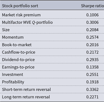
This table summarizes the long-term Sharpe ratio for each stock portfolio strategy in the period from January 1964 to December 2013. The Sharpe ratio is the ratio of excess stock return to its standard deviation. The basket of stock portfolio strategies encompasses the CRSP value-weighted market portfolio, the multifactor mean-variance efficient (MMVE) tangency stock portfolio from the Fama and French (Reference Fama and French2015) joint return spreads for size, value, investment, and profitability, as well as the ubiquitous asset pricing anomalies such as size, value (book-to-market, cashflow-to-price, dividend-to-price, and earnings-to-price), momentum, investment, profitability, short-term return reversal, and long-term return reversal. The Sharpe ratios land in the range of 0.1006 for the CRSP value-weighted market portfolio to 0.3006 for the multifactor MVE tangency portfolio and 0.3362 for the short-term return reversal strategy. The other Sharpe ratios land within this intermediate range.
3.2 Time-varying dynamic conditional alphas
Table 3 presents the time-varying Fama and French (Reference Fama and French2015) alphas across the deciles for each of the portfolio sorts, t-tests of these alpha spreads between the extreme deciles with the Newey-West (1987) standard-error correction that safeguards against potential heteroskedasticity and serial correlation, F-tests of mean-variance efficiency (Gibbons et al. (Reference Gibbons, Ross and Shanken1989)), and Q-tests that we propose as the appropriate test of dynamic portfolio efficiency to complement the filter. A first glance at Table 3 indicates that most dynamic conditional alphas are statistically close to nil. Out of these portfolio tilts, only the momentum, short-term reversal, and long-term reversal tilts yield significant alpha spreads between the top and bottom deciles in the range of 0.989, –1.180, and 0.426 (p-values < 0.001). Yet, the positive sign of the average alpha spread for long-term return reversal is counter-intuitive and therefore instead suggests long-term return momentum. This evidence contradicts the prior studies in support of long-term return reversal that can arise from the typical investor’s naïve extrapolation of past superior stock performance (DeBondt and Thaler (Reference DeBondt and Thaler1985); Lakonishok et al. (Reference Lakonishok, Shleifer and Vishny1994); Fama and French (Reference Fama and French1996)). With respect to return momentum (Jegadeesh and Titman (Reference Jegadeesh and Titman1993, Reference Jegadeesh and Titman2001); Chan et al. (Reference Chan, Jegadeesh and Lakonishok1996)), the long-term average dynamic conditional alpha is significant only for the extreme deciles. In this case, the top and bottom deciles produce significant average conditional alphas of –0.569 and 0.42 respectively (p-values < 0.005). The resultant alpha spread is therefore significant at the conventional statistical confidence level. Also, the dynamic conditional alpha spread between the extreme short-term reversal deciles is significant in econometric terms (p-value < 0.001). Whether these results are a statistical aberration calls for more formal hypothesis tests on the short-term reversal and momentum phenomena.
Table 3. Average dynamic alphas, dynamic alpha spreads, NW t-tests, AGRS F-tests, AGMM $\chi$
2
tests, and MMVE Q-tests
$\chi$
2
tests, and MMVE Q-tests

Over the 50-year period from January 1964 to December 2013, the econometrician applies the recursive multivariate Filter to extract dynamic factor premiums from the Fama and French (Reference Fama and French2015) five-factor asset pricing model. At each time increment, the econometrician takes into account the Fama and French (Reference Fama and French2015) factors such as the excess return on the market portfolio (MRP), the return spread between the top 30% small and bottom 30% big stocks (SMB), the return spread between the top 30% high book-to-market and bottom 30% low book-to-market stocks (HML), the return spread between the top 30% robust and bottom 30% weak stocks in terms of their relative profitability (RMW), and the return spread between the top 30% conservative investment and bottom 30% aggressive investment stocks (CMA) to explain the variation in the excess return on each stock decile for size, momentum, value (cf. book-to-market, cashflow-to-price, dividend-to-price, and earnings-to-price), investment, profitability, short-term return reversal, and long-term return reversal. The econometrician presents the mathematical time-series representation below:
 \begin{equation*} R_{kt}-R_{ft}=\alpha _{t}+\beta _{mt}\!\left(R_{mt}-R_{ft}\right)+\beta _{st}SMB_{t}+\beta _{ht}HML_{t}+\beta _{rt}RMW_{t}+\beta _{ct}CMA_{t}+\varepsilon _{t} \end{equation*}
Table 3 sums up the long-run average alpha for each stock decile sorted on size, value, momentum, investment, profitability, short-term return reversal, and long-term return reversal. The first 10 columns summarize each long-run average alpha and its corresponding p-value for the null hypothesis of zero dynamic alpha. The next column encapsulates the long-run average alpha spread for the long-short trading strategy that involves both a long position in the top decile and a short position in the bottom decile throughout the 50-year period from January 1964 to December 2013. The last three columns summarize the Gibbons et al. (Reference Gibbons, Ross and Shanken1989) AGRS F-test, AGMM C-test, and AGMM Q-test results on each long-short trading strategy across the ubiquitous asset pricing anomalies such as size, value, momentum, investment, profitability, short-term return reversal, and long-term return reversal. This evidence reports each test statistic and its corresponding p-value. For each hypothesis test, the econometrician applies the Newey and West (Reference Newey and West1987) method with quadratic spectral kernel estimation to correct the standard errors to safeguard against any serial correlation and heteroskedasticity. The appendix depicts the time-series dynamic alphas for each of the stock portfolio tilts that yield anomalous excess returns in static asset pricing analysis (i.e. size, value, momentum, investment, profitability, short-term return reversal, and long-term return reversal).
In Table 3, all the AGRS F-tests, the AGMM C-tests, and the Q-tests unanimously suggest that dynamic conditional alphas are jointly indistinguishable from zero for all the portfolio tilts. The p-values are substantially near unity across the board. Hence, there is minimal evidence in support of the alternative hypothesis that our dynamic factor model is incorrectly specified. The main economic intuition is that the wedge between the Sharpe-ratio squares for the benchmark portfolio and the long-short decile strategy is not large enough to justify the statistical rejection of a dynamic variant of the Fama and French (Reference Fama and French2015) factor model. The conditional factor premiums are too volatile for the econometrician to affirm the consistent outperformance of each portfolio tilt once he or she takes into account the dynamic nature of these conditional factor premiums. In Appendix 1, the time-series visualization of dynamic conditional alpha spreads between both the top and bottom deciles corroborates this empirical fact. A falsification test suggests that the highest F-test, C-test, and Q-test p-value is 0.04 (not shown in the tables and charts) when we exclude any one of the Fama and French (Reference Fama and French2015) explanatory factors from the recursive estimation. This falsification test evidence supports the joint insignificant of dynamic conditional alphas.
Harvey et al. (Reference Harvey, Liu and Zhu2016) introduce a multiple testing framework (e.g. Harvey and Liu (Reference Harvey and Liu2014a, Reference Harvey and Liu2014b, Reference Harvey and Liu2014c, Reference Harvey and Liu2014d)) and provide a unique variety of historical significance cut-offs from the first empirical tests in the 1960s to the present. This new strand of investment literature suggests that we should raise the test hurdle substantially from a t-ratio of 2.0 to a t-ratio of 3.0 for most cross-sectional asset-pricing tests. Specifically, Harvey et al. (Reference Harvey, Liu and Zhu2016) find that this higher hurdle reduces the number of cross-sectional anomalies from 316 to only 2 that is, value and momentum (cf. Asness et al. (Reference Asness, Moskowitz and Pedersen2013); Fama and French (Reference Fama and French2016); Hou et al. (Reference Hou, Xue and Zhang2017)). In addition, Harvey et al. (Reference Harvey, Liu and Zhu2016) propose that a theoretically-derived factor should have a lower hurdle than an empirically-discovered factor. Their central thesis suggests that a factor can be important in some economic environments but unimportant in some other environments.
While our econometric innovation complements Harvey et al. (Reference Harvey, Liu and Zhu2016) multiple testing analysis, our work serves as a time-series equivalent to their cross-sectional adjustment for asset-pricing tests. Back-of-the-envelope calculations show that the typical stock portfolio’s Sharpe ratio has to increase by at least 3 to 8.2 times for most dynamic conditional alphas to be jointly significant at the conventional confidence level. The critical values for the $\chi$
2-test with 525 degrees of freedom are 603.31, 579.43, and 566.91 at the respective 99%, 95%, and 90% confidence levels. Table 3 demonstrates that the highest C-test or Q-test statistic is 59.29 while the lowest C-test or Q-test statistic is 8.97. Therefore, the smallest Sharpe ratio multiplier can be calculated as (566.932/59.29)1/2 = 3.092 while the largest Sharpe ratio multiplier can then be calculated as (603.31/8.97)1/2 = 8.201. As a result, the econometrician has to specify a higher test hurdle for each anomaly. Across the deciles, most dynamic conditional alphas need to be larger on average with significantly less variability for the Sharpe ratio to increase by at least 3 to 8 times. The equivalent Sharpe ratio would be in the approximate range of 1.15 to 2.4 (cf. Kozak et al. (Reference Kozak, Nagel and Santosh2017)). In other words, our unique dynamic analysis of conditional factor premiums proposes raising the bar for the econometric asset pricing test. This recommendation echoes the cross-sectional counterpart of Harvey et al. (Reference Harvey, Liu and Zhu2016).
$\chi$
2-test with 525 degrees of freedom are 603.31, 579.43, and 566.91 at the respective 99%, 95%, and 90% confidence levels. Table 3 demonstrates that the highest C-test or Q-test statistic is 59.29 while the lowest C-test or Q-test statistic is 8.97. Therefore, the smallest Sharpe ratio multiplier can be calculated as (566.932/59.29)1/2 = 3.092 while the largest Sharpe ratio multiplier can then be calculated as (603.31/8.97)1/2 = 8.201. As a result, the econometrician has to specify a higher test hurdle for each anomaly. Across the deciles, most dynamic conditional alphas need to be larger on average with significantly less variability for the Sharpe ratio to increase by at least 3 to 8 times. The equivalent Sharpe ratio would be in the approximate range of 1.15 to 2.4 (cf. Kozak et al. (Reference Kozak, Nagel and Santosh2017)). In other words, our unique dynamic analysis of conditional factor premiums proposes raising the bar for the econometric asset pricing test. This recommendation echoes the cross-sectional counterpart of Harvey et al. (Reference Harvey, Liu and Zhu2016).
3.3 ARMA-GARCH representation of each dynamic conditional factor premium
In this section, we demonstrate that each dynamic conditional factor premium can be modeled as a financial time-series. We apply both ARMA(1,1)-EGARCH(1,1,1) and ARMA(1,1)-GJR-GARCH(1,1,1) conditional-mean-and-variance models to fit each conditional factor premium that the econometrician extracts from a dynamic variant of the Fama and French (Reference Fama and French2015) multifactor model. Although it is possible to identify a better time-series representation for each conditional factor premium, our goal here is more straight-forward. In fact, our primary objective is to apply the standard toolkit in time-series econometrics to establish the empirical fact that each dynamic alpha or beta spread exhibits the major properties of most financial time series. Each conditional factor premium embeds autoregressive mean reversion in the conditional mean specification of ARMA(1,1), and volatility clusters and asymmetries in the conditional volatility specification of EGARCH(1,1,1) or GJR GARCH(1,1,1) (cf. Engle (Reference Engle1982); Bollerslev (Reference Bollerslev1986); Nelson (Reference Nelson1991); Glosten et al. (Reference Glosten, Jagannathan and Runkle1993)):
ARMA(1,1) conditional mean specification
 \begin{equation} m_{t}=a+bm_{t-1}+cw_{t-1}+w_{t} \end{equation}
 \begin{equation} w_{t}=\sqrt{h_{t}}\varepsilon _{t} \end{equation}
EGARCH(1,1,1) and GJR-GARCH (1,1,1) conditional variance specifications
 \begin{equation} h_{t}=\exp \!\left\{d+e\!\left(\frac{w_{t}}{\sqrt{h_{t-1}}}\right)+f\ln h_{t-1}+g\!\left(\left| \frac{w_{t}}{\sqrt{h_{t-1}}}\right| -\left| \frac{E\!\left(w_{t}\right)}{\sqrt{h_{t-1}}}\right| \right)\right\} \end{equation}
 \begin{equation} h_{t}=d+ew_{t-1}^{2}+fh_{t-1}+gD_{t-1}w_{t-1}^{2} \end{equation}
where m
t is the dynamic conditional alpha or beta spread; w
t is the residual error term; h
t is the conditional variance process; $\varepsilon$
t is a Gaussian white noise; D
t denotes a binary variable with a numerical value of unity if w
t is negative or zero if w
t is positive; a, b, c, d, e, f, and g are the parameters for quasi-maximum likelihood estimation. The canonical ARMA model serves as the conditional mean specification to capture any autoregressive mean reversion in the dynamic conditional alpha or beta spread between the extreme deciles, while EGARCH or GJR-GARCH fits the conditional variance specification to encapsulate any volatility clusters and asymmetries in the current factor premium time-series under study.
$\varepsilon$
t is a Gaussian white noise; D
t denotes a binary variable with a numerical value of unity if w
t is negative or zero if w
t is positive; a, b, c, d, e, f, and g are the parameters for quasi-maximum likelihood estimation. The canonical ARMA model serves as the conditional mean specification to capture any autoregressive mean reversion in the dynamic conditional alpha or beta spread between the extreme deciles, while EGARCH or GJR-GARCH fits the conditional variance specification to encapsulate any volatility clusters and asymmetries in the current factor premium time-series under study.
It is important to draw a distinction between this time-series analysis and the prior studies of multiple conditional factor models (Ferson and Harvey (Reference Ferson and Harvey1991, Reference Ferson and Harvey1999); Fama and French (Reference Fama and French2006); Ang and Chen (Reference Ang and Chen2007); Ang and Kristensen (Reference Ang and Kristensen2012)). In the current study, we need not impose any a priori assumption about the dynamic evolution of conditional alpha or beta spreads, whereas, the earlier studies of conditional factor models make specific assumptions about the time-series behaviors of dynamic conditional factor premiums (such as structural breaks in autoregressive mean reversion). Yet, the econometrician can readily fit an ARMA-EGARCH or ARMA-GJR-GARCH model to characterize the dynamic evolution of each conditional alpha or beta spread over time. This characterization entails both reasonable and flexible assumptions about the true conditional mean and variance processes for each dynamic conditional factor premium.
This time-series analysis also differs from several earlier studies that exclusively focus on the CAPM (cf. Adrian and Franzoni (Reference Adrian and Franzoni2009); Ang and Chen (Reference Ang and Chen2007); Lewellen and Nagel (Reference Lewellen and Nagel2006)). The recursive multivariate filter helps extract dynamic conditional alphas and betas from the Fama and French (Reference Fama and French2015) multifactor model, and then the econometrician can apply equations (14)–(17) to model each dynamic conditional alpha or beta spread as a typical financial time series. While it is reasonable to identify the “best” ARMA-GARCH representation for each conditional alpha or beta spread, we aim to establish the empirical fact that each conditional alpha or beta spread exhibits most prevalent properties of a typical financial time series. In turn, this empirical fact defies the conventional wisdom of point estimates of factor premiums in most static time-series ordinary least-squares regressions. Table 4 summarizes the empirical results in Appendix 2 (cf. Tables A2.1 to A2.6).
Table 4. ARMA-GARCH time-series representation of each dynamic conditional alpha and beta spread

This table summarizes the empirical results in Appendix 2 (cf. Tables A2.1 to A2.6). We demonstrate that each dynamic conditional factor premium can be modeled as a typical financial time-series. We apply both ARMA(1,1)-EGARCH(1,1,1) and ARMA(1,1)-GJR-GARCH(1,1,1) conditional-mean-and-variance models to fit each factor premium that the econometrician extracts from a “dynamic” variant of the Fama and French (Reference Fama and French2015) factor model. Although it is possible to identify a more precise time-series representation for each factor premium, our goal here is more straight-forward. In fact, our primary and ultimate goal is to use the standard toolkit in time-series econometrics to establish the empirical fact that each dynamic conditional alpha or beta spread exhibits the major properties of most financial time series. Each factor premium embeds autoregressive mean reversion in the conditional mean specification of ARMA(1,1), as well as volatility clusters and asymmetries in the conditional volatility specification of EGARCH(1,1,1) or GJR-GARCH(1,1,1) (cf. Engle (Reference Engle1982); Bollerslev (Reference Bollerslev1986); Nelson (Reference Nelson1991); Glosten et al (Reference Glosten, Jagannathan and Runkle1993)).
We summarize several bullet points from Appendix 2 and the tabular results therein:
-
1. These results allow us to establish the empirical fact that almost all the dynamic conditional factor premiums exhibit the key properties of most financial time-series. Specifically, these dynamic conditional alpha and beta spreads exhibit autoregressive mean reversion in the conditional mean specification, and volatility clusters and asymmetries in the conditional variance specification. Therefore, the conditional moments of factors and returns manifest in the form of state-dependent alphas and betas, or dynamic conditional factor premiums, across Fama and French’s (Reference Fama and French2015; 2016) fundamental factors (Nagel and Singleton (Reference Nagel and Singleton2011)). Our subsequent analysis suggests bilateral causation between macroeconomic surprises and conditional alpha spreads. Overall, the evidence enriches our chosen interpretation of the intertemporal CAPM that most macroeconomic gyrations both lead and covary with the conditional expectations of terminal wealth in the investor’s investment opportunity set (cf. Merton (Reference Merton1973); Campbell (Reference Campbell1993); Fama (Reference Fama1996); Campbell and Vuolteenaho (Reference Campbell and Vuolteenaho2004), Campbell et al. (Reference Campbell, Polk and Vuolteenaho2009); Campbell et al. (Reference Campbell, Giglio, Polk and Turley2017)). To the extent that macroeconomic shocks manifest in the form of persistent dynamic conditional alpha spreads, mutual causation between macro surprises and alpha spreads hence becomes an informative piece of evidence that we can exploit in order to resolve at least some of the prevalent abnormal returns or stock market anomalies.
-
2. To the extent that stock market information serves as a useful indicator of macro surprises, each dynamic conditional factor premium conveys rich information about macroeconomic growth, market valuation, financial stress, cyclical variation, or forecast combination. This inference calls for more corroboration in the core spirit of several recent studies (Liew and Vassalou (Reference Liew and Vassalou2000); Vassalou (2003); Vassalou and Xing (2004); Petkova (Reference Petkova2006); Campbell et al. (Reference Campbell, Polk and Vuolteenaho2009); Campbell et al. (Reference Campbell, Giglio, Polk and Turley2017)).
-
3. Most of the average conditional alpha spreads are insignificant while the exceptions are momentum and short-term reversal (with absolute t-ratios more than 2.9). For the latter portfolio tilts, the respective conditional average alpha spreads are 1.03 and –1.12. These conditional mean alpha spreads are close to the corresponding average dynamic conditional alpha spreads for momentum and short-term return reversal of 0.989 and –1.18 in Table 3. Although these average alpha spreads seem to persist in the extreme deciles (cf. Fama and French (Reference Fama and French2008; 2016)), it is key to recall the more formal Sharpe ratio test evidence that the average alphas do not jointly differ from nil across all the momentum and short-term return reversal deciles. In other words, these dynamic conditional alphas are too volatile for one to reject the hypothesis that our chosen dynamic version of the Fama and French (Reference Fama and French2015) factor model is a correct specification. The logic leads the econometrician to infer that the average alpha spreads are consistent between Table 3 and Table A2.1.
-
4. Table A2.3 shows that each dynamic conditional HML beta exhibits much variability over time for the original Fama-French value factor to be economically meaningful in explaining time variation in average stock returns. In conjunction with the evidence of significant long-term average HML betas in Table A5.3, the ARMA-GARCH results support the use of HML as a relevant state variable that helps better span the investor’s mean-variance space. Thus, HML conveys non-negligible information about at least some variation in average returns for a wide variety of stock portfolio tilts. This major inference reconciles with some recent independent empirical contributions of Fama and French (Reference Fama and French2015, Reference Fama and French2016) and Hou et al. (Reference Hou, Xue and Zhang2015): HML appears to be redundant once the econometrician incorporates RMW and CMA into the factor model for the U.S. stock market, whereas, the hefty value premium persists both in the U.S. and several other stock markets (Asness et al. (Reference Asness, Moskowitz and Pedersen2013); Fama and French (Reference Fama and French2016)). In turn, the economic content and substance of HML and even SMB may help explain whether these state variables serve as useful empirical proxies for macroeconomic innovations (Liew and Vassalou (Reference Liew and Vassalou2000), Vassalou (2003); Petkova (Reference Petkova2006); Hahn and Lee (Reference Hahn and Lee2006)), distress risk (Griffin and Lemmon (Reference Griffin and Lemmon2002); Vassalou and Xing (2004)), or some other behavioral mispricing reasons (Campbell et al. (Reference Campbell, Hilscher and Szilagyi2008)). Our subsequent evidence generalizes the key empirical inference that mutual causation between macroeconomic surprises and dynamic conditional alpha spreads can be an informative and plausible economic explanation for most anomalies in the fundamental evolution of average returns and factors.
3.4 Conditional specification test evidence
In this section, we derive and design a new conditional specification test to differentiate the static and dynamic conditional models. Under the null hypothesis, both the static and dynamic conditional estimators are consistent and asymptotically normal while the former attains the Cramer-Rao lower bound and therefore is efficient in the standard econometric nomenclature with the parameter vector $\theta$
={
$\theta$
={ $\alpha$
,
$\alpha$
, $\beta$
m,
$\beta$
m, $\beta$
s,
$\beta$
s, $\beta$
h,
$\beta$
h, $\beta$
r,
$\beta$
r, $\beta$
c}. In contrast, only the dynamic conditional estimator is consistent under the alternative hypothesis. For our subsequent derivation, we define the distance between the static and dynamic conditional estimators as
$\beta$
c}. In contrast, only the dynamic conditional estimator is consistent under the alternative hypothesis. For our subsequent derivation, we define the distance between the static and dynamic conditional estimators as $\boldsymbol\xi = \boldsymbol\theta_{d}-\boldsymbol\theta_{s}$
. The null hypothesis suggests a trivial distance between the static and dynamic conditional estimators:
$\boldsymbol\xi = \boldsymbol\theta_{d}-\boldsymbol\theta_{s}$
. The null hypothesis suggests a trivial distance between the static and dynamic conditional estimators:
 \begin{equation} \hat{\boldsymbol{\xi }}=\hat{\boldsymbol{\theta }}_{d}-\hat{\boldsymbol{\theta }}_{s}\Rightarrow H_{0}\colon \boldsymbol{\theta }_{d}=\boldsymbol{\theta }_{s}\Rightarrow H_{0}\colon \boldsymbol{\xi }=0 \end{equation}
We define the variance-covariance matrix for the main distance between each estimator and its respective true parameter vector
V
s and
V
d where equations (1) and (2) carry the Gaussian normal error terms $\varepsilon$
t and e
t:
$\varepsilon$
t and e
t:
 \begin{equation} N^{1/2}\cdot \left(\hat{\boldsymbol{\theta }}_{s}-\boldsymbol{\theta }_{s}\right)\sim N\!\left(0,{\boldsymbol{{V}}}_{s}\right) \end{equation}
 \begin{equation} N^{1/2}\cdot \left(\hat{\boldsymbol{\theta }}_{d}-\boldsymbol{\theta }_{d}\right)\sim N\!\left(0,{\boldsymbol{{V}}}_{d}\right) \end{equation}
The proof begins with the naïve assumption the static estimator is not orthogonal to the distance between the static and dynamic conditional estimators. Then, the mathematical derivation leads to a contradiction to affirm the alternative scenario that the static estimator is indeed orthogonal to the vector wedge between the static and dynamic conditional estimators. The key crux of this simple proof relies on the Cramer-Rao lower-bound efficiency criterion that the vector distance between the static and dynamic variance-covariance matrices must be positive-semidefinite. In fact, we can use a unique algorithm to handle the rare case where the vector distance is negative-semidefinite. We first define the dynamic conditional estimator as the static estimator plus some multiple of the above vector wedge in equation (18) while the latter term must be zero under the null hypothesis (where we expect the scalar k = 0 with the probability limit plim $\boldsymbol\xi$
= 0 under the null hypothesis that both static and dynamic conditional estimators are asymptotically equivalent):
$\boldsymbol\xi$
= 0 under the null hypothesis that both static and dynamic conditional estimators are asymptotically equivalent):
 \begin{equation} \hat{\boldsymbol{\theta }}_{{\boldsymbol{{d}}}}=\hat{\boldsymbol{\theta }}_{{\boldsymbol{{s}}}}+\textit{k}{\boldsymbol{{M}}}\hat{\boldsymbol{\xi }} \end{equation}
where k is a scalar and M is a chosen matrix. Next, we expand the variance-covariance matrix for the dynamic conditional estimator:
 \begin{equation} {\boldsymbol{{V}}}\!\left(\hat{\boldsymbol{\theta }}_{d}\right)={\boldsymbol{{V}}}\!\left(\hat{\boldsymbol{\theta }}_{s}\right)+k{\boldsymbol{{MQ}}}+k{\boldsymbol{{M}}}^{T}{\boldsymbol{{Q}}}^{T}+k^{2}{\boldsymbol{{MV}}}\!\left(\hat{\boldsymbol{\xi }}\right){\boldsymbol{{M}}}^{T}\Rightarrow {\boldsymbol{{Q}}}=\mathrm{cov}\!\left(\hat{\boldsymbol{\theta }}_{s},\hat{\boldsymbol{\xi }}\right) \end{equation}
We can also expand the vector wedge between the respective variance-covariance matrices for the static and dynamic conditional estimators:
 \begin{equation} {\boldsymbol{{W}}}\!\left(k\right)={\boldsymbol{{V}}}\!\left(\hat{\boldsymbol{\theta }}_{d}\right)-{\boldsymbol{{V}}}\!\left(\hat{\boldsymbol{\theta }}_{s}\right)=k{\boldsymbol{{MQ}}}+k{\boldsymbol{{Q}}}^{T}{\boldsymbol{{M}}}^{T}+k^{2}{\boldsymbol{{MV}}}\!\left(\hat{\boldsymbol{\xi }}\right){\boldsymbol{{M}}}^{T} \end{equation}
We derive the first-order and second-order derivatives of this vector wedge with respect to k:
 \begin{equation} \nabla _{k}{\boldsymbol{{W}}}\!\left(k\right)={\boldsymbol{{MQ}}}+{\boldsymbol{{Q}}}^{T}{\boldsymbol{{M}}}^{T}+2k{\boldsymbol{{MV}}}\!\left(\hat{\boldsymbol{\xi }}\right){\boldsymbol{{M}}}^{T} \end{equation}
 \begin{equation} \nabla _{k}^{2}{\boldsymbol{{W}}}\!\left(k\right)=2{\boldsymbol{{MV}}}\!\left(\hat{\boldsymbol{\xi }}\right){\boldsymbol{{M}}}^{T} \end{equation}
Equation (25) suggests that the second-order derivative is positive definite. As a result, one can figure out the minimum vector wedge when he or she sets the first-order condition (24) to zero:
 \begin{equation} \nabla _{k}{\boldsymbol{{W}}}\!\left(k\right)={\boldsymbol{{MQ}}}+{\boldsymbol{{Q}}}^{T}{\boldsymbol{{M}}}^{T}+2k{\boldsymbol{{MV}}}\!\left(\hat{\boldsymbol{\xi }}\right){\boldsymbol{{M}}}^{T}=0\Rightarrow {\boldsymbol{{M}}}=-\left(2k{\boldsymbol{{V}}}\!\left(\hat{\boldsymbol{\xi }}\right)\right)^{-1}{\boldsymbol{{Q}}}^{T} \end{equation}
By definition, we know the equality W (k = 0)=0. When we evaluate the first-order derivative at k = 0, this resultant matrix cannot be positive-semidefinite:
 \begin{equation} \nabla _{k}{\boldsymbol{{W}}}\!\left(k=0\right)={\boldsymbol{{MQ}}}+{\boldsymbol{{Q}}}^{T}{\boldsymbol{{M}}}^{T}=-\left(2k{\boldsymbol{{V}}}\!\left(\hat{\boldsymbol{\xi }}\right)\right)^{-1}2{\boldsymbol{{Q}}}^{T}{\boldsymbol{{Q}}}=-\left(k{\boldsymbol{{V}}}\!\left(\hat{\boldsymbol{\xi }}\right)\right)^{-1}{\boldsymbol{{Q}}}^{T}{\boldsymbol{{Q}}} \end{equation}
Equation (27) suggests that the resultant matrix must not be positive-semidefinite. This solution poses a contradiction to the assumption that W (k) must be positive-semidefinite. For arbitrarily small values of k, equation (27) suggests that W (k) can be negative-semidefinite. In turn, this contradiction suggests that Q equates a null matrix. Therefore, we can find zero covariance between the static estimator and its distance from the dynamic conditional estimator.
This analytical result allows us to derive a new dynamic conditional specification test in a similar spirt of the econometric contributions of Durbin (Reference Durbin1954), Wu (1973), Hausman (Reference Hausman1978), Nakamura and Nakamura (Reference Nakamura and Nakamura1981), White (1982), Newey (Reference Newey1985), and Tauchen (1985).
 \begin{equation} \hat{\boldsymbol{\xi }}=\hat{\boldsymbol{\theta }}_{d}-\hat{\boldsymbol{\theta }}_{s}\Rightarrow \hat{\boldsymbol{\xi }}+\hat{\boldsymbol{\theta }}_{s}=\hat{\boldsymbol{\theta }}_{d}\Rightarrow {\boldsymbol{{V}}}\!\left(\hat{\boldsymbol{\xi }}\right)+{\boldsymbol{{V}}}\!\left(\hat{\boldsymbol{\theta }}_{s}\right)={\boldsymbol{{V}}}\!\left(\hat{\boldsymbol{\theta }}_{d}\right)\Rightarrow {\boldsymbol{{V}}}\!\left(\hat{\boldsymbol{\xi }}\right)={\boldsymbol{{V}}}\!\left(\hat{\boldsymbol{\theta }}_{d}\right)-{\boldsymbol{{V}}}\!\left(\hat{\boldsymbol{\theta }}_{s}\right) \end{equation}
 \begin{equation} \kappa =\hat{\boldsymbol{\xi }}^{T}\!\left(T^{-1}\hat{{\boldsymbol{{V}}}}\!\left(\hat{\boldsymbol{\xi }}\right)\right)^{-1}\hat{\boldsymbol{\xi }}=T\cdot \hat{\boldsymbol{\xi }}^{T}\!\left({\boldsymbol{{V}}}\!\left(\hat{\boldsymbol{\theta }}_{d}\right)-{\boldsymbol{{V}}}\!\left(\hat{\boldsymbol{\theta }}_{s}\right)\right)^{-1}\hat{\boldsymbol{\xi }}\sim \chi ^{2}\!\left(q\right) \end{equation}
where q denotes the number of parameters as the degrees of freedom for the $\chi$
2 test statistic and T denotes the number of time periods over the entire data span.
$\chi$
2 test statistic and T denotes the number of time periods over the entire data span.
While this dynamic conditional specification test statistic shares the same sandwich form of most econometric tests, the middle matrix may or may not always be positive-semidefinite. This occurrence arises from the rare but plausible case where the static OLS estimator contains much measurement noise that the dynamic conditional estimator becomes similar in terms of efficiency. In this rare case, we need to adjust this unconventional middle matrix to the nearest positive definite matrix (Higham (Reference Higham2002)). This algorithmic approach entails setting any negative eigenvalues to zero to re-approximate the positive-definite matrix. Although we sometimes run this algorithm to carry out the dynamic conditional specification test, this extreme but plausible scenario is rather rare. When this scenario occurs in practice, the resultant dynamic conditional specification test statistics may not exceed the critical value and so there is insufficient evidence to differentiate the static and dynamic estimators. In practice, our conditional specification test rejects the null hypothesis of a correct static model for at least 95% of all the stock decile tilts. This rejection suggests that the alternative dynamic conditional alpha model yields consistent estimates of factor premiums.
Table 5 lists the conditional specification test evidence in favor of the dynamic conditional multifactor asset pricing model. In our empirical analysis of 100 monthly decile returns on the major anomalies plus their respective 10 long-short portfolios that focus on the extreme deciles, 95% of the portfolio tilts suggest the statistical rejection of the null hypothesis that the static factor model is a correctly specification. The preponderance of empirical results supports the dynamic conditional factor model in stark contrast to the static baseline model for good reasons. First, the vast majority of dynamic conditional alphas are statistically insignificant so that most of the pricing errors are close to zero in the alternative dynamic conditional model specification. Second, the conditional specification test results prevail in favor of the alternative hypothesis that only the dynamic conditional estimator is consistent. This latter point highlights the power of measurement error minimization that the recursive multivariate filter achieves for consistent statistical estimation. Overall, the dynamic conditional factor model can outperform its static counterpart in light of the conditional specification test evidence and dynamic conditional alpha insignificance.Footnote 4
Table 5. Conditional specification test of the static versus dynamic conditional multifactor asset pricing models

Over the 50-year period from January 1964 to December 2013, one applies the recursive multivariate Filter to extract dynamic multifactor factor premiums from the Fama and French (Reference Fama and French2015) five-factor asset pricing model. At each time increment, the econometrician takes into account the Fama and French (Reference Fama and French2015) factors such as the excess return on the market portfolio (MRP), the return spread between the top 30% small and bottom 30% big stocks (SMB), the return spread between the top 30% high book-to-market and bottom 30% low book-to-market stocks (HML), the return spread between the top 30% robust and bottom 30% weak stocks in terms of their relative profitability (RMW), and the return spread between the top 30% conservative investment and bottom 30% aggressive investment stocks (CMA) to explain the variation in the excess return on each stock decile for size, momentum, value (cf. book-to-market, cashflow-to-price, dividend-to-price, and earnings-to-price), investment, profitability, short-term return reversal, and long-term return reversal. The econometrician presents the mathematical time-series representation below:.
 \begin{equation*} R_{kt}-R_{ft}=\alpha _{t}+\beta _{mt}\!\left(R_{mt}-R_{ft}\right)+\beta _{st}SMB_{t}+\beta _{ht}HML_{t}+\beta _{rt}RMW_{t}+\beta _{ct}CMA_{t}+\varepsilon _{t} \end{equation*}
Table 5 presents the conditional specification test evidence for each stock decile sorted on size, value, momentum, asset investment, operating profitability, short-term return reversal, and long-term return reversal. The first 10 columns summarize the $\chi$
2-statistic for each stock decile and its corresponding p-value for the null hypothesis of a consistent and efficient static estimator against the alternative hypothesis of a correct consistent dynamic conditional estimator. The next column shows the
$\chi$
2-statistic for each stock decile and its corresponding p-value for the null hypothesis of a consistent and efficient static estimator against the alternative hypothesis of a correct consistent dynamic conditional estimator. The next column shows the $\chi$
2-statistic for each long-short top-bottom stock decile and its corresponding p-value. About 95% of the
$\chi$
2-statistic for each long-short top-bottom stock decile and its corresponding p-value. About 95% of the $\chi$
2-statistics are econometrically significant with at least 90%+ confidence. The appendix depicts the dynamic conditional alpha time-series for each of the stock portfolio tilts that yield anomalous excess returns in static asset pricing analysis (i.e. size, value, momentum, asset investment, operating profitability, short-term return reversal, and long-term return reversal).
$\chi$
2-statistics are econometrically significant with at least 90%+ confidence. The appendix depicts the dynamic conditional alpha time-series for each of the stock portfolio tilts that yield anomalous excess returns in static asset pricing analysis (i.e. size, value, momentum, asset investment, operating profitability, short-term return reversal, and long-term return reversal).
 \begin{align*} \hat{\boldsymbol{\xi }}=\hat{\boldsymbol{\theta }}_{d}-\hat{\boldsymbol{\theta }}_{s}\Rightarrow H_{0}\colon \boldsymbol{\theta }_{d}=\boldsymbol{\theta }_{s}\Rightarrow H_{0}\colon \boldsymbol{\xi }=0 \end{align*}
 \begin{align*} N^{1/2}\cdot (\hat{\boldsymbol{\theta }}_{s}-\boldsymbol{\theta }_{s})\sim N(0,{\boldsymbol{{V}}}_{s})\quad N^{1/2}\cdot (\hat{\boldsymbol{\theta }}_{d}-\boldsymbol{\theta }_{d})\sim N(0,{\boldsymbol{{V}}}_{d}) \end{align*}
 \begin{equation*} \hat{\boldsymbol{\xi }}=\hat{\boldsymbol{\theta }}_{d}-\hat{\boldsymbol{\theta }}_{s}\Rightarrow \hat{\boldsymbol{\xi }}+\hat{\boldsymbol{\theta }}_{s}=\hat{\boldsymbol{\theta }}_{d}\Rightarrow {\boldsymbol{{V}}}\!\left(\hat{\boldsymbol{\xi }}\right)+{\boldsymbol{{V}}}\!\left(\hat{\boldsymbol{\theta }}_{s}\right)={\boldsymbol{{V}}}\!\left(\hat{\boldsymbol{\theta }}_{d}\right)\Rightarrow {\boldsymbol{{V}}}\!\left(\hat{\boldsymbol{\xi }}\right)={\boldsymbol{{V}}}\!\left(\hat{\boldsymbol{\theta }}_{d}\right)-{\boldsymbol{{V}}}\!\left(\hat{\boldsymbol{\theta }}_{s}\right) \end{equation*}
 \begin{equation*} \kappa =\hat{\boldsymbol{\xi }}^{T}\!\left(T^{-1}\hat{{\boldsymbol{{V}}}}\!\left(\hat{\boldsymbol{\xi }}\right)\right)^{-1}\hat{\boldsymbol{\xi }}=T\cdot \hat{\boldsymbol{\xi }}^{T}\!\left({\boldsymbol{{V}}}\!\left(\hat{\boldsymbol{\theta }}_{d}\right)-{\boldsymbol{{V}}}\!\left(\hat{\boldsymbol{\theta }}_{s}\right)\right)^{-1}\hat{\boldsymbol{\xi }}\sim \chi ^{2}\!\left(q\right) \end{equation*}
Therefore, both the recursive multivariate filter and dynamic conditional specification test add value to the econometric toolkit for subsequent asset-pricing analysis. Not only does this econometric advancement pose a core conceptual challenge to the conventional use of ordinary least-squares (OLS) regressions for factor model design, but this econometric innovation also suggests that dynamic conditional alpha estimation serves as a useful quantitative method for financial applications such as mutual fund performance evaluation, corporate event assessment, equity cost estimation, and financial risk management.
4. Mutual causation between macroeconomic innovations and alpha spreads
In this section, we delve into the main crux of the current study and empirically ascertain mutual causation between macroeconomic innovations and dynamic conditional alpha spreads. To the extent that macroeconomic innovations manifest in the form of these dynamic conditional alpha spreads, this causality reveals the marginal investor’s fundamental news and expectations about the cross-section of average returns. We interpret this Granger-causality evidence in the broader context of the intertemporal CAPM with cash-flow news, discount-rate news, as well as future- risk news (cf. Merton (Reference Merton1973); Campbell (Reference Campbell1993); Campbell and Vuolteenaho (Reference Campbell and Vuolteenaho2004); Campbell et al. (Reference Campbell, Giglio, Polk and Turley2017)). Campbell and Vuolteenaho (Reference Campbell and Vuolteenaho2004) develop the intertemporal CAPM with cash-flow and discount-rate betas. Campbell et al. (Reference Campbell, Giglio, Polk and Turley2017) extend and generalize the intertemporal CAPM with stochastic volatility to capture future-risk news. The price of risk for cash-flow news is the marginal investor’s relative risk aversion coefficient times more than the unit price of risk for negative discount-rate news. Therefore, cash-flow news carries “bad betas”, whereas, negative discount-rate news carries “good betas”. Also, an asset that provides positive returns when future risk expectations increase tends to generate low average returns. Thus, the marginal investor’s stochastic discount factor is high when he or she anticipates high stochastic volatility in the future. In essence, these fundamental news and expectations reflect the marginal investor’s rational response to different kinds of macroeconomic surprises with respect to cash flows, discount rates, and stochastic volatilities. Vector autoregressions (VAR) and Granger-causality tests below accord with the main theme of bilateral causation between macroeconomic innovations and dynamic conditional alphas. This causation reinforces the intertemporal asset- pricing interpretation that macroeconomic shocks manifest in the form of dynamic conditional factor premiums and vice versa such that this nexus reveals the marginal investor’s fundamental news and macroeconomic expectations about the cross-section of average returns. To the extent that these causal relations reflect the marginal investor’s rational response to changes in his or her intertemporal choice and conditional expectation of terminal wealth, the resultant dynamic conditional factor model differentiates itself from most behavioral mispricing models. This key conceptual distinction resonates with the primary thesis of Kozak et al. (Reference Kozak, Nagel and Santosh2018) recent critique of numerous horseraces for empirically-driven factor models.
We use 15 main monthly time-series in a macroeconometric vector autoregression (VAR) (Sims (1980); Campbell (Reference Campbell1993)). There are 12 macro time-series, 2 financial uncertainty metrics, and 2 investor sentiment proxies. The resultant dataset spans the 285-month sample period from April 1990 to December 2013. These macrofinancial time-series include first differences in the national economic activity index, Treasury bill rate, unemployment rate, term spread, default spread, prime bank loan rate, aggregate equity market dividend yield, as well as percent changes in industrial production, non-farm payroll, house price index, consumer price index, exchange rate, financial stress index, economic policy uncertainty, and investor sentiment. For the Baker- Wurgler capital market investor sentiment index, we use the first principal component as a main empirical proxy. This variable choice has no impact on our subsequent inferences. Table 6 lists and describes these macroeconomic variable definitions and their data sources.
Table 6. Macroeconomic variable definitions and their data sources

This table describes the macroeconomic variable definitions and their public data sources in our vector autoregression analysis of Granger mutual causation between fundamental macro surprises and dynamic conditional factor premiums. To the extent that macro surprises manifest in the form of dynamic conditional factor premiums, this Granger causation reveals the marginal investor’s fundamental news and rational expectations about the cross-section of average returns.
We specify 15 major monthly time-series in a standard macroeconometric vector autoregressive system. There are 12 macroeconomic variables, 2 financial uncertainty time-series, and 2 investor sentiment proxies. For the Baker-Wurgler investor sentiment index, we use the original first principal component as a better empirical proxy. The resultant dataset spans the 285-month sample period from April 1990 to December 2013. These macroeconomic time-series include changes in the national economic activity index, Treasury bill rate, unemployment rate, term spread, default spread, prime bank loan rate, aggregate equity market dividend yield, and percent changes in U.S. industrial production, non-farm payroll, house price index, consumer price index, exchange rate, financial stress index, economic policy uncertainty, and investor sentiment.
We develop a medium macroeconometric vector autoregressive system in order to gauge macroeconomic innovations or fundamental surprises that the typical investor would face in his or her investment journey. Insofar as we can gauge macroeconomic surprises, we establish the empirical fact of mutual Granger causation between macroeconomic innovations and dynamic conditional alpha spreads. Granger-causality tests help us assess this mutual causation as a core qualifying condition for fundamental factor selection.
Table 7 shows the vector autoregression (VAR) coefficient estimates and t-statistics. This VAR model explains most of the time variation in fundamental macroeconomic news. The only exception is the macro VAR model of percent changes in the economic policy uncertainty index (Baker et al. (2016)), which seems to contain peculiar information in its own right. Due to its unique lag structure, the Baker and Wurgler (2007) financial market investor sentiment VAR model generates the highest R 2 of 94.9%. This macroeconometric VAR system captures reasonably well time variation in U.S. national economic activity, prime bank loan interest rate, non-farm payroll, and residential house price index with intermediate R 2s from 40% to 68%.
Table 7. Vector AutoRegression (VAR) of macroeconomic fluctuations with consistent coefficient estimates and t-statistics

This table summarizes the macroeconometric vector autoregression (VAR) results. The upper panel presents the consistent coefficient estimates, and the lower panel shows the corresponding t-statistics. We use 15 main monthly time-series in a macroeconometric vector autoregressive system (Sims (1980); Campbell (Reference Campbell1993)). There are 12 macro time-series, 2 financial uncertainty metrics, and 2 investor sentiment proxies. The resultant dataset spans the 285-month sample period from April 1990 to December 2013. These macro time-series encompass first differences in the national economic activity index, Treasury bill rate, unemployment rate, term spread, default spread, prime bank loan rate, aggregate dividend yield, and percent changes in industrial production, non-farm payroll, house price index, consumer price index, exchange rate, financial stress index, economic policy uncertainty, and investor sentiment. Appendix 3 presents and describes the macroeconomic variable definitions and their data sources.
This macroeconometric VAR system explains about 20–30% of time variation in each of the other key macroeconomic time-series such as the Treasury 3-month bill rate, unemployment rate, term spread, default spread, aggregate dividend yield, industrial production, dollar strength, CPI inflation, and systemic stress within the U.S. financial sector. Overall, this medium macro VAR system allows us to extract macroeconomic innovations (or fundamental surprises) as the residual disturbances from each of the resultant macro equations.
Tables 8 and 9 list the pairwise Granger causality tests with p-values for us to see whether there is mutual causation between macroeconomic surprises and dynamic conditional alphas. Indeed, these test results suggest the affirmative case for Granger causation in both directions. Table 8 shows that at least 1 to 4 macroeconomic innovations Granger-cause each dynamic conditional alpha spread for size, value (B/M, CF/P, and Div/P), operating profitability, asset growth, short-term return reversal, and long-run return reversal. Only momentum and partial value (E/P) turn out to be the exceptions that defy this rule of thumb.
Table 8. Granger causation from macroeconomic innovations to dynamic conditional alpha spreads

This table shows the pairwise Granger-causality test p-values for the econometrician to assess whether Granger causation runs from macroeconometric innovations to dynamic conditional alphas. The columns indicate the respective asset pricing anomalies such as size, momentum, value (B/M, CF/P, Div/P, and E/P), asset growth, operating profitability, short-run return reversal, and long-run return reversal. This tables demonstrates that at least a few macro innovations Granger-cause each dynamic conditional alpha spread with at least 90% statistical confidence (p-values < 0.10) for most anomalies such as size, value (B/M, CF/P, and Div/P), asset growth, operating profitability, short-run return reversal, and long-term reversal. Only momentum and partial value (E/P) turn out to be the exceptions that defy this rule of thumb. Within the intertemporal CAPM context, we interpret this evidence in support of the prevalent use of Fama and French (Reference Fama and French2015) factors in a dynamic conditional model. Granger causation between macroeconomic innovations and dynamic conditional alphas serves as a core qualifying condition for “shrinking the factor zoo”, whereas, there is minimal evidence in favor of viewing momentum as a conceptually sound fundamental factor in the dynamic conditional context. To the extent that the investor cannot decipher fundamental news nor macroeconomic surprises from momentum, it remains hard to rationalize momentum apart from a unique statistical aberration. Insofar as momentum returns persist as an anomaly, we need a more plausible explanation than behavioral mispricing disequilibrium before we view momentum as an extra fundamental factor in the dynamic conditional model.
Table 9. Granger causation from dynamic conditional alpha spreads to macroeconomic innovations

This table shows the pairwise Granger-causality test p-values for the econometrician to assess whether Granger causation runs from dynamic conditional alphas to macroeconometric innovations. The columns indicate the respective asset pricing anomalies such as size, momentum, value (B/M, CF/P, Div/P, and E/P), asset growth, operating profitability, short-run return reversal, and long-run return reversal. Only partial value (Div/P and E/P), asset growth, operating profitability, short-run return reversal, and long-run reversal exhibit this reverse causation (p-values < 0.10). In fact, the primary conditional alpha spreads for size, value (B/M and CF/P), and momentum convey little causal information about macroeconomic innovations (p-values > 0.10). Within the intertemporal CAPM context, we interpret this evidence in support of the prevalent use of Fama and French (Reference Fama and French2015) fundamental factors in a dynamic conditional model. Granger causation between macroeconomic innovations and dynamic conditional alphas serves as a core qualifying condition for “shrinking the factor zoo”, whereas, there is minimal evidence in favor of viewing momentum as a conceptually sound fundamental factor in the dynamic conditional context. To the extent that the investor cannot decipher fundamental news nor macroeconomic surprises from momentum, it remains hard to rationalize momentum apart from a unique statistical aberration. Insofar as momentum profits persist as an anomaly, we need a more plausible explanation than behavioral mispricing disequilibrium before we view momentum as an extra fundamental factor in the dynamic conditional model.
Table 9 shows that reverse causality runs from several dynamic conditional alpha spreads to macroeconomic innovations. Key conditional alpha spreads represent rich and valuable stock market signals about macroeconomic surprises. However, this evidence is less conclusive since only partial value (Div/P and E/P), asset investment growth, operating profitability, short-term return reversal, and long-term return reversal exhibit this reverse causation. In fact, the primary conditional alpha spreads for size, value (B/M and CF/P), and momentum convey little causal information about macroeconomic innovations.
We retain our main focus on the recursive multivariate filtration of Fama-French dynamic conditional alphas. The subsequent GARCH and VAR results complement and corroborate this focus. For this reason, we would like to draw attention to mutual causation between conditional alphas and macro innovations in Table 9.Footnote 5 Specifically, many stock market alphas help predict macroeconomic surprises: partial value alpha spreads Div/P and E/P show this critical causation. This evidence resonates with the title of the current study. We highlight this reverse causation in Table 9 while the vector autoregression results in Table 8 support the conventional view that macroeconomic surprises Granger-cause at least some stock market alphas.
On balance, these results suggest mutual Granger causation from macroeconomic surprises to most dynamic conditional alpha spreads and vice versa (except momentum and partial value). Within the intertemporal CAPM context, we interpret this evidence in support of the prevalent use of Fama and French (2015) factors in a dynamic conditional model. Mutual causation between macroeconomic innovations and dynamic conditional alpha spreads serves as a core qualifying condition for “shrinking the factor zoo”, whereas, there is minimal or no sufficient evidence in favor of viewing momentum as a conceptually sound factor in the dynamic conditional context. To the extent that the marginal investor cannot decipher fundamental news nor macroeconomic surprises from momentum, it is difficult to rationalize momentum apart from a unique statistical aberration. Insofar as momentum profits persist as an anomaly, we need a more plausible reason than behavioral mispricing disequilibrium before we view momentum as an extra fundamental factor in the dynamic conditional model.
Tables 8 and 9 demonstrate bilateral causation between most macroeconomic shocks and dynamic conditional alpha spreads. To the extent that macroeconomic innovations manifest in the form of these dynamic conditional alpha spreads, this critical channel of Granger causation reveals the marginal investor’s fundamental news and expectations about the cross-section of average returns. This core evidence enriches and contributes to our chosen intertemporal asset- pricing interpretation of dynamic conditional factor models. In this intertemporal asset-pricing context, macroeconomic innovations serve as fundamental news and surprises that induce cash- flow betas and future-risk betas as “bad betas” or negative discount-rate betas as “good betas”. In accordance with this intertemporal CAPM thesis, we would expect assets with positive cash- flow shocks, future-risk spillovers, or subpar discount-rate news to generate low average returns. Conversely, we would expect other assets with negative cash-flow surprises, volatility declines, or optimistic discount-rate news to generate high average returns. Therefore, mutual causation between macroeconomic innovations and dynamic conditional alpha spreads serves as a core qualifying condition for more effective factor selection with sound economic rigor and intuition. This new economic insight is one of our key contributions to modern asset pricing model design. Appendix 4 discusses the main similarities and differences between our current study and some concurrent contributions.
In accordance with the core thesis of Kozak et al. (Reference Kozak, Nagel and Santosh2018), both fundamental and behavioral factors can help price the cross-section of average returns. In order to determine whether a specific factor is fundamental, the econometrician can measure factor covariances or factor premiums with macroeconomic risk innovations. Vector autoregression (VAR) evidence confirms bilateral Granger causation between dynamic conditional alphas and macroeconomic risk innovations. VAR evidence further supports this mutual causation for Fama and French (Reference Fama and French2015) fundamental factors with the plausible exceptions of both momentum and partial value. In light of this evidence, it would be informative to analyze the dynamic conditional alpha time-series (cf. Appendix 1 time-series visualization of dynamic conditional alphas). When each dynamic conditional alpha is nil on average but can be persistently positive and negative during different phases of the real business cycle, the conditional moments and factor premiums can help inform empirical asset pricing model design and performance.
Our dynamic analysis of core conditional factor premiums from the Fama and French (Reference Fama and French2015) model proposes raising the hurdle for the conventional asset-pricing test. This recommendation serves as the time-series equivalent to the cross-sectional thesis of Harvey et al. (Reference Harvey, Liu and Zhu2016). Also, our prime empirical analysis contradicts McLean and Pontiff’s (Reference McLean and Pontiff2016) recent conjecture that academic research partially erodes stock return predictability because investors are able to learn from a variety of anomalies. To the extent that the dynamic conditional factor premiums exhibit substantial volatility over time, the vast majority of dynamic conditional alphas are not significantly far from zero while there is no sufficient evidence to reject the hypothesis that our conditional factor model carries a correct specification. For this reason, we can reconcile most ubiquitous anomalies with a dynamic variant of the Fama-French factor model. Also, our study offers a mild refutation of Berk and Van Binsbergen’s (Reference Berk and Van Binsbergen2016) and Barber et al. (Reference Barber, Huang and Odean2016) overall qualitative conclusion that the CAPM is the clear victor in the horserace against the other dynamic-equilibrium and factor models. In contrast, our work shows that the dynamic conditional factor model provides progress toward a positive portrayal of the quantitative nexus between average return and risk. Our dynamic conditional factor model helps draw a distinction between both rational-risk and behavioral theories of average return evolution because bilateral causation between macroeconomic innovations and dynamic conditional alpha spreads shines unique light on the marginal investor’s fundamental news and economic expectations about the cross-section of average returns. This insight offers economic logic, rigor, and intuition for our empirical analysis in response to the recent landmark statistical discovery of Kozak et al. (Reference Kozak, Nagel and Santosh2018). As a consequence, the myriad contributions of our current study help address at least part of the concern and suspicion in the recent reappraisals of asset pricing model tests (cf. Lewellen et al. (Reference Lewellen, Nagel and Shanken2010); Berk and van Binsbergen (Reference Berk and Van Binsbergen2016); Barber et al. (Reference Barber, Huang and Odean2016); Harvey et al. (Reference Harvey, Liu and Zhu2016); Fama and French (Reference Fama and French2015, Reference Fama and French2016); Kozak et al. (Reference Kozak, Nagel and Santosh2017, Reference Kozak, Nagel and Santosh2018)).
5. Conclusion
In response to Kozak et al. (Reference Kozak, Nagel and Santosh2018) recent critique of many horseraces among factor models, we apply a new approach to addressing at least part of the concern and suspicion in several reappraisals of asset pricing tests (cf. Lewellen et al. (Reference Lewellen, Nagel and Shanken2010); Berk and van Binsbergen (Reference Berk and Van Binsbergen2016); Barber et al. (Reference Barber, Huang and Odean2016); Harvey et al. (Reference Harvey, Liu and Zhu2016); Fama and French (Reference Fama and French2015, Reference Fama and French2016); Kozak et al. (Reference Kozak, Nagel and Santosh2017, Reference Kozak, Nagel and Santosh2018)). We extract dynamic conditional factor premiums from the Fama and French (Reference Fama and French2015) model and then find that most anomalies disappear after one accounts for time variation in these premiums. Mutual causation between dynamic conditional alpha spreads and macroeconomic surprises serves as a core qualifying condition for relevant fundamental factor selection with sound economic rigor and motivation. To the extent that macroeconomic innovations manifest in the form of dynamic conditional alphas, this causation reveals the marginal investor’s fundamental news and macroeconomic expectations about the cross-section of average returns.
Specifically, our evidence bolsters the ubiquitous use of Fama and French (Reference Fama and French2015) factors that reflect the marginal investor’s response to fundamental news about the cross-section of average returns. Our econometric results lend credence to Fama and French’s (Reference Fama and French1996, Reference Fama and French2004, Reference Fama and French2008, Reference Fama and French2015, Reference Fama and French2016) perennial reluctance to encompass Carhart (Reference Carhart1997) momentum in their factor model. In a conceptual domain, we link the dynamic conditional factor model results to recent advances in the intertemporal CAPM context (Merton (Reference Merton1973); Campbell (Reference Campbell1993); Campbell and Vuolteenaho (Reference Campbell and Vuolteenaho2004); Campbell et al. (Reference Campbell, Giglio, Polk and Turley2017)). Overall, our current study serves as an incremental step toward better deciphering a distinction between the rational risk and behavioral mispricing paradigms.
The ARMA-GARCH conditional mean-variance specifications and vector autoregressions (VAR) are important in the current study. The ARMA-GARCH part is important because we can apply these conditional mean-variance models to yield dynamic conditional alpha forecasts to help predict future macroeconomic fluctuations. Further, the VAR part is important because we can establish mutual causation between dynamic alphas and macro innovations. In turn, this mutual causation serves as a core qualifying condition for valid and effective fundamental factor selection. In combination, the resultant econometric tests and results bolster our empirical response to the recent critique by Kozak et al. (Reference Kozak, Nagel and Santosh2017 and Reference Kozak, Nagel and Santosh2018): the fundamental factors would covary with macroeconomic fluctuations (but the behavioral mispricing factors would not). As a consequence, our empirical work helps draw a distinction between the rational risk and behavioral strands of macroeconomic assets return prediction.
We agree with Kozak et al. (Reference Kozak, Nagel and Santosh2018) qualitative conclusion on “observational equivalence between most rational risk factor models and behavioral mispricing factor models”. As we have discussed in the introduction of the current study, this consensus resonates with the relentless debate and elusive quest of a factor model for our profession. These advances shed new light on the major essential need for financial economists to “[develop-and-test] structural asset-pricing models with specific assumptions about investor beliefs and preferences that can deliver testable predictions about (1) the fundamental factors that should be in the [stochastic discount factor] (SDF), and (2) the probability distributions under which this SDF prices assets” (Kozak et al. Reference Kozak, Nagel and Santosh2018).
A concurrent contribution moves in this direction. Yeh (2021) derives and estimates the SDF from financial intermediary capital strength and then uses the Euler, asset return prediction, and price multiple valuation equations to test stock market anomaly persistence over a broad basket of long-short extreme decile strategies. Yeh (2021) further tests the empirical predictions of the dynamic stochastic general equilibrium (DSGE) structural model to find evidence in support of his permanent capital hypothesis. This new frontier shows some promise in applying “structural macrofinance models” of both investor beliefs and preferences for economists to make progress in macroeconomic asset return prediction.
Visualization: Dynamic conditional alphas for the extreme deciles
This visualization shows the time-series charts of the Fama-French dynamic conditional alphas for the extreme deciles for the stock portfolio tilts such as size, value, momentum, profitability, investment, short-run return reversal, and long-run return reversal. These dynamic factor premiums exhibit wide variation for the top and bottom deciles. Some large comovements tend to influence the central tendency of the alpha spread between the extreme deciles. Each alpha spread often switches its sign and becomes econometrically insignificant. In addition to Gibbons et al. (Reference Gibbons, Ross and Shanken1989) AGRS F-test, the AGMM C-test and AGMM Q-test of dynamic multifactor mean-variance efficiency (MMVE) suggests that the average alpha spreads are not different from zero. The distance between the squared Sharpe ratios for each individual stock portfolio and the MMVE tangency portfolio is not large enough for one to reject the null hypothesis of a correct asset pricing model specification. This inference accords with the spirit of the intertemporal context of Merton (Reference Merton1973), Campbell (Reference Campbell1993), and Fama (Reference Fama1996). Investors care about not only their terminal wealth but also several behavioral considerations such as human capital, labor income, consumption, and hedging investment opportunities that covary with the conditional expectations of their terminal wealth. In this light, the Fama and French (Reference Fama and French2015) factors serve as valid and relevant state variables that reflect these co-movements in response to the typical investor’s demand for hedging instruments. To the extent that the dynamic factor premiums on each Fama and French (Reference Fama and French2015) state variable is econometrically significant across the entire data span (i.e. each dynamic multifactor beta consistently differs from zero), the resultant dynamic alpha exhibits too much variability for the pricing error to be significant enough for the econometrician to reject the null hypothesis that the dynamic multi-factor model specification is correct.

Supplementary material
To view supplementary material for this article, please visit http://doi.org/10.1017/S1365100523000184


 Open access