

1. Introduction
Seemingly unrelated regression (SUR) models include several individual units that are linked by the fact that their disturbances are correlated. The correlation among the equation disturbances could come from several sources, such as correlated technological shocks, tax policy changes, or credit crunches, which may affect all individual units together. Consequently, such models have been broadly used in econometrics and applied works. Using the correlation among the equations in SUR models, one can improve the efficiency of estimates compared to those obtained by an equation-by-equation least squares, see Zellner (Reference Zellner1962). However, standard estimators in SUR are arguably restrictive, as they assume that the slope coefficients are constant over time. As an economy may experience an unexpected shock across time (such as oil price shocks, financial crises, or technological shocks), and such a shock is likely to have impact on economic variables simultaneously, it is important to consider structural breaks in SUR models. This is a critical issue to consider because structural breaks are an important source of forecast failures in macroeconomics and finance as documented by Pesaran and Timmermann (Reference Pesaran and Timmermann2002, Reference Pesaran and Timmermann2007), Pesaran et al. (Reference Pesaran, Pettenuzzo and Timmermann2006), Clements and Hendry (Reference Clements and Hendry2006, Reference Clements and Hendry2011), Giacomini and Rossi (Reference Giacomini and Rossi2009), Inoue and Rossi (Reference Inoue and Rossi2011), Pesaran and Pick (Reference Pesaran and Pick2011), Pesaran et al. (Reference Pesaran, Pick and Pranovich2013), Rossi (Reference Rossi and Part2013), Barnett et al. (Reference Barnett, Chauvet and Leiva-Leon2016), and Lee et al. (Reference Lee, Parsaeian and Ullah2022, Reference Lee, Parsaeian and Ullah2022a), among others. To deal with this challenge, this paper considers structural breaks in SUR models and develops estimation and forecasting methods in this framework.
There has been a recent increase in literature concerning the estimation and tests of common breaks in panel data models with a main focus on the detection of break points and their asymptotic properties. Large $N$
and
$N$
and $T$
panels involve nuisance parameters that increase at a quadratic rate because the cross-section dimension of the panel is allowed to rise. One solution to deal with this issue is to restrict the covariance matrix of the errors using a common factor specification with a fixed number of unobserved factors, as discussed in Bai and Ng (Reference Bai and Ng2002), Coakley et al. (Reference Coakley, Fuertes and Smith2002), and Phillips and Sul (Reference Phillips and Sul2003), to mention a few. Despite the considerable attention to the detection of break points, only a few studies have attempted to forecast panel data models, see Smith and Timmermann (Reference Smith and Timmermann2018), Smith (Reference Smith and Timmermann2018), and Liu (Reference Liu2022) which use a Bayesian framework. Our paper differs from their work in that it considers the so-called frequentist model averaging framework, which relies on the data on hand. Further, the main purpose of our paper is to find a more accurate estimate of the slope parameters in the sense of mean squared errors (MSEs) and also optimal forecast in the sense of mean squared forecast errors (MSFE) in SUR models.Footnote
1
$T$
panels involve nuisance parameters that increase at a quadratic rate because the cross-section dimension of the panel is allowed to rise. One solution to deal with this issue is to restrict the covariance matrix of the errors using a common factor specification with a fixed number of unobserved factors, as discussed in Bai and Ng (Reference Bai and Ng2002), Coakley et al. (Reference Coakley, Fuertes and Smith2002), and Phillips and Sul (Reference Phillips and Sul2003), to mention a few. Despite the considerable attention to the detection of break points, only a few studies have attempted to forecast panel data models, see Smith and Timmermann (Reference Smith and Timmermann2018), Smith (Reference Smith and Timmermann2018), and Liu (Reference Liu2022) which use a Bayesian framework. Our paper differs from their work in that it considers the so-called frequentist model averaging framework, which relies on the data on hand. Further, the main purpose of our paper is to find a more accurate estimate of the slope parameters in the sense of mean squared errors (MSEs) and also optimal forecast in the sense of mean squared forecast errors (MSFE) in SUR models.Footnote
1
This paper develops two averaging estimators in SUR models for estimating the slope coefficients and forecasting under structural breaks when the cross-section dimension is fixed while the time dimension is allowed to increase without bounds. It is important to allow for large $T$
because, for example, technological changes or policy implementations are likely to happen over long time horizons. Moreover, the model allows for the cross-sectional dependence to gain from the correlation across individuals, which is not applicable in a univariate time series model. Ignoring cross-sectional dependence of errors can have serious consequences and can result in misleading inference and even inconsistent estimators, depending on the extent of the cross-sectional dependence. This cross-correlations could arise due to omitted common effects, spatial effects, or as a result of interactions within socioeconomic networks, as discussed in Chudick and Pesaran (Reference Chudick and Pesaran2015).
$T$
because, for example, technological changes or policy implementations are likely to happen over long time horizons. Moreover, the model allows for the cross-sectional dependence to gain from the correlation across individuals, which is not applicable in a univariate time series model. Ignoring cross-sectional dependence of errors can have serious consequences and can result in misleading inference and even inconsistent estimators, depending on the extent of the cross-sectional dependence. This cross-correlations could arise due to omitted common effects, spatial effects, or as a result of interactions within socioeconomic networks, as discussed in Chudick and Pesaran (Reference Chudick and Pesaran2015).
Our first proposed estimator is a weighted average of an unrestricted estimator and a restricted estimator in which the averaging weight takes the form of the James-Stein weight, cf. Stein (Reference Stein1956) and James and Stein (Reference James and Stein1961).Footnote 2 The restricted estimator is built under the restriction of no break in the coefficients, that is, the coefficients across different regimes are restricted to be the same as if there were no structural break. Therefore, the restricted estimator will be biased when there is a break, but is the most efficient one. However, the unrestricted estimator considers the break points and only uses the observations within each regime to estimate the coefficients. Thus, the unrestricted estimator is consistent but less efficient. The weighted average of the unrestricted estimator and the restricted estimator therefore balances the trade-off between the bias and the variance efficiency depending on the magnitude of the break. We establish the asymptotic risk for the Stein-like shrinkage estimator and show that its asymptotic risk is smaller than that of the unrestricted estimator, which is the common method for estimating the slope coefficients under structural breaks. We note that this out-performance comes from the efficiency of the restricted estimator in which it exploits the observations in neighboring regime(s). Therefore, the proposed estimator provides a better estimate and ultimately a better forecast in the sense of MSFE.
The second proposed estimator is a weighted average of the unrestricted estimator and the restricted estimator in which the averaging weight is derived by minimizing the asymptotic risk. This estimator is called the minimal MSE estimator. We derive the asymptotic risk of the minimal MSE estimator and show that it is smaller than the asymptotic risk of the unrestricted estimator. In addition, we analytically compare its asymptotic risk with that of the Stein-like shrinkage estimator. The results show the out-performance of the Stein-like shrinkage estimator over the minimal MSE estimator under small break sizes. However, for large break sizes or large number of regressors, both estimators have almost equal performance. It is noteworthy that both of the proposed estimators uniformly outperform the unrestricted estimator, in the sense of having a smaller asymptotic risk, for any break size and break point. When choosing between the two proposed estimators, based on the analytical and numerical results, we recommend the Stein-like shrinkage estimator as it uniformly outperforms or performs as well as the minimal MSE estimator.Footnote 3
We conduct a Monte Carlo simulation study to evaluate the performance of the proposed averaging estimators. The results confirm the theoretically expected improvements in the Stein-like shrinkage estimator and the minimal MSE estimator over the unrestricted estimator for any break size and break point. Further, we provide an empirical analysis of forecasting output growth rates of G7 countries using quarterly data from 1995:Q1 to 2016:Q4. Our empirical results show the benefits of using the proposed averaging estimators over the unrestricted estimator and other alternative estimators.
This paper is structured as follows. Section 2 presents the SUR model under the structural break. Section 3 introduces the Stein-like shrinkage estimator, as well as its asymptotic distribution and asymptotic risk. This section also introduces the minimal MSE estimator and compares the asymptotic risk of this estimator with that of the Stein-like shrinkage estimator. Section 4 reports the Monte Carlo simulation. Section 5 presents the empirical analysis. Section 6 concludes the paper. Detailed proofs are provided in Appendix A.
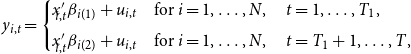
2. The model
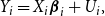
Consider the following heterogeneous SUR model
 \begin{equation} y_{i,t}=x'_{\!\!i,t} \beta _{i}+ u_{i,t}, \quad \text{for} \ i=1, \dots, N, \quad t=1, \dots, T, \end{equation}
where $x_{i,t}$
is a
$x_{i,t}$
is a $k \times 1$
vector of regressors, and
$k \times 1$
vector of regressors, and $u_{i,t}$
is the error term with zero mean that is allowed to have cross-sectional dependence as well as heteroskedasticity. The vector of coefficients,
$u_{i,t}$
is the error term with zero mean that is allowed to have cross-sectional dependence as well as heteroskedasticity. The vector of coefficients, $\beta _i$
, and the variance of the error term,
$\beta _i$
, and the variance of the error term, $u_{i,t}$
, are subject to a common break across individuals at time
$u_{i,t}$
, are subject to a common break across individuals at time $T_1$
, where
$T_1$
, where $b_1 \equiv T_1/T \in (0, 1)$
, such that
$b_1 \equiv T_1/T \in (0, 1)$
, such that
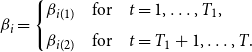 \begin{equation} \beta _{i}= \begin{cases} \beta _{i(1)} & \mbox{for} \quad t=1, \dots, T_1, \\[5pt] \beta _{i(2)} & \mbox{for} \quad t=T_1+1, \dots, T. \end{cases} \end{equation}
Let $Y_i, X_i, U_i$
denote the stacked data and errors for individuals
$Y_i, X_i, U_i$
denote the stacked data and errors for individuals $i=1, \dots, N$
over the time period observed. Then,
$i=1, \dots, N$
over the time period observed. Then,
 \begin{equation} Y_i= X_i \boldsymbol{\beta }_i+U_i, \end{equation}
where $Y_i= \big ( y'_{\!\!i(1)}, y'_{\!\!i(2)}\big )'$
is a vector of
$Y_i= \big ( y'_{\!\!i(1)}, y'_{\!\!i(2)}\big )'$
is a vector of $T \times 1$
dependent variable, with
$T \times 1$
dependent variable, with $y_{i(1)}= \big (y_{i,1}, \dots, y_{i,T_1}\big )'$
and
$y_{i(1)}= \big (y_{i,1}, \dots, y_{i,T_1}\big )'$
and $y_{i(2)}= \big (y_{i,T_1+1}, \dots, y_{i,T}\big )'$
. Also,
$y_{i(2)}= \big (y_{i,T_1+1}, \dots, y_{i,T}\big )'$
. Also, $X_i=\text{diag}\big (x_{i(1)}, x_{i(2)}\big )$
is a
$X_i=\text{diag}\big (x_{i(1)}, x_{i(2)}\big )$
is a $T \times 2k$
diagonal matrix in which
$T \times 2k$
diagonal matrix in which $x_{i(1)}= \big (x_{i,1}, \dots, x_{i,T_1}\big )'$
and
$x_{i(1)}= \big (x_{i,1}, \dots, x_{i,T_1}\big )'$
and $x_{i(2)}=\big (x_{i,T_1+1}, \dots, x_{i,T}\big )'$
.
$x_{i(2)}=\big (x_{i,T_1+1}, \dots, x_{i,T}\big )'$
. $\boldsymbol{\beta }_i= \big (\beta' _{\!\!i(1)}, \beta' _{\!\!i(2)}\big )'$
is a
$\boldsymbol{\beta }_i= \big (\beta' _{\!\!i(1)}, \beta' _{\!\!i(2)}\big )'$
is a $2k \times 1$
vector of the slope coefficients, and
$2k \times 1$
vector of the slope coefficients, and $U_i= \big (u_{i(1)}, u_{i(2)} \big )'$
is a
$U_i= \big (u_{i(1)}, u_{i(2)} \big )'$
is a $T \times 1$
vector of error terms with
$T \times 1$
vector of error terms with $u_{i(1)}= \big (u_{i,1}, \dots, u_{i,T_1}\big )'$
and
$u_{i(1)}= \big (u_{i,1}, \dots, u_{i,T_1}\big )'$
and $u_{i(2)}= \big (u_{i,T_1+1}, \dots, u_{i,T}\big )'$
. It is convenient to stack the equations over
$u_{i(2)}= \big (u_{i,T_1+1}, \dots, u_{i,T}\big )'$
. It is convenient to stack the equations over $N$
individuals as
$N$
individuals as
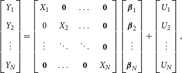 \begin{equation} \begin{bmatrix} Y_1 \\[5pt] Y_2 \\[5pt] \vdots \\[5pt] Y_N \end{bmatrix}= \left[\begin{array}{c@{\quad}c@{\quad}c@{\quad}c} X_1 & \mathbf{0} & \dots & \mathbf{0}\\[5pt] 0 & X_2 & \dots & \mathbf{0} \\[5pt] \vdots & \ddots & \ddots & \mathbf{0} \\[5pt] \mathbf{0} & \dots & \mathbf{0} & X_N \end{array}\right] \begin{bmatrix} \boldsymbol{\beta }_1 \\[5pt] \boldsymbol{\beta }_2 \\[5pt] \vdots \\[5pt] \boldsymbol{\beta }_N \end{bmatrix}+\begin{bmatrix} U_1 \\[5pt] U_2 \\[5pt] \vdots \\[5pt] U_N \end{bmatrix}, \end{equation}
or compactly in matrix notation as
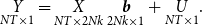 \begin{equation} \underset{NT \times 1}{Y}= \underset{NT \times 2Nk}{X} \ \underset{2Nk \times 1}{\boldsymbol{{b}}} + \underset{NT \times 1}{U}. \end{equation}
We make the following assumptions:
ASSUMPTION 1. $\{(\widetilde{x}_t, \widetilde{u}_t)\}$
is an i.i.d. sequence where
$\{(\widetilde{x}_t, \widetilde{u}_t)\}$
is an i.i.d. sequence where $\widetilde{x}_t=\text{diag}\big (x'_{\!\!1,t}, \dots, x'_{\!\!N,t}\big )$
,
$\widetilde{x}_t=\text{diag}\big (x'_{\!\!1,t}, \dots, x'_{\!\!N,t}\big )$
, $\widetilde{u}_t=\big (u_{1,t}, \dots, u_{N,t} \big )',$
and
$\widetilde{u}_t=\big (u_{1,t}, \dots, u_{N,t} \big )',$
and ${\mathbb{E}}(\widetilde{u}_t| \widetilde{x}_t)=0.$
ASSUMPTION 2. The disturbances are heteroscedastic across regimes and are uncorrelated across time but correlated across individual equations,
 \begin{equation} Var(U)\equiv \Omega =\left[\begin{array}{c@{\quad}c@{\quad}c@{\quad}c} \Omega _{11} & \Omega _{12} & \dots & \Omega _{1N} \\[5pt] \Omega _{21} & \Omega _{22} & \dots & \Omega _{2N} \\[5pt] \vdots & \vdots & \ddots & \vdots \\[5pt] \Omega _{N1} & \Omega _{N2}& \dots & \Omega _{NN} \end{array}\right] \end{equation}
where $\Omega _{ij}= \begin{bmatrix} \text{cov} \big (u_{i(1)},u_{j(1)}\big ) & \mathbf{0} \\[5pt] \mathbf{0}& \text{cov} \big (u_{i(2)},u_{j(2)}\big ) \end{bmatrix}= \begin{bmatrix} \sigma _{ij(1)} I_{T_1}& \mathbf{0} \\[5pt] \mathbf{0} & \sigma _{ij(2)} I_{(T-T_1)} \end{bmatrix}.$
ASSUMPTION 3.
The product moment matrix $\big (\frac{X' \Omega ^{-1} X}{T} \big )$
has full rank and tends to a finite non-singular matrix as
$\big (\frac{X' \Omega ^{-1} X}{T} \big )$
has full rank and tends to a finite non-singular matrix as $T \rightarrow \infty$
.
$T \rightarrow \infty$
.
We note that Assumption 1 implies that the observations are not correlated across time so that conventional central limit theory applies. Assumption 2 implies the cross-sectional dependence across individuals. Assumption 3 guarantees that the generalized least squares (GLS) estimation method used in Section 3 is uniquely defined.
We note that the method of break point estimation is based on the least-squares principle discussed in Bai and Perron (Reference Bai and Perron2003) for a univariate time series model, and the extensions to the multivariate regression setting are described in Qu and Perron (Reference Qu and Perron2007). It has been shown that the estimated break fraction, $\widehat{b}_1$
, converges to its true value,
$\widehat{b}_1$
, converges to its true value, $b_1$
, at a rate that is fast enough not to affect the
$b_1$
, at a rate that is fast enough not to affect the $\sqrt{T}$
consistency of the estimated parameters asymptotically, see Qu and Perron (Reference Qu and Perron2007).
$\sqrt{T}$
consistency of the estimated parameters asymptotically, see Qu and Perron (Reference Qu and Perron2007).
3. The proposed averaging estimators
This section introduces the Stein-like shrinkage estimator and the minimal MSE estimator. We also provide an analytical comparison of the two proposed estimators.
3.1. Stein-like shrinkage estimator
For the estimation of the slope parameters in model (5), we propose the Stein-like shrinkage estimator that can reduce the estimation error under structural breaks. Our proposed shrinkage estimator denoted by $\widehat{\boldsymbol{{b}}}_{w}$
is
$\widehat{\boldsymbol{{b}}}_{w}$
is
 \begin{equation} \widehat{\boldsymbol{{b}}}_{w} ={w_T} \widehat{\boldsymbol{{b}}}_{ur}+ (1-{w_T}) \widehat{\boldsymbol{{b}}}_{r}, \end{equation}
where $\widehat{\boldsymbol{{b}}}_{r}$
is called the restricted estimator, which is under the restriction of no break in the coefficients. Thus, it estimates the parameters by ignoring the break. Therefore, the restricted estimator is biased when there is a break while it is efficient. The unrestricted estimator,
$\widehat{\boldsymbol{{b}}}_{r}$
is called the restricted estimator, which is under the restriction of no break in the coefficients. Thus, it estimates the parameters by ignoring the break. Therefore, the restricted estimator is biased when there is a break while it is efficient. The unrestricted estimator, $\widehat{\boldsymbol{{b}}}_{ur}$
, estimates the coefficients by considering the common break point across all individuals, so this is the unbiased estimator but less efficient. As a result, the weighted average of the restricted and unrestricted estimators trades off between the bias and variance efficiency. The shrinkage weight takes the form of
$\widehat{\boldsymbol{{b}}}_{ur}$
, estimates the coefficients by considering the common break point across all individuals, so this is the unbiased estimator but less efficient. As a result, the weighted average of the restricted and unrestricted estimators trades off between the bias and variance efficiency. The shrinkage weight takes the form of
 \begin{equation} w_T= \Big (1- \frac{\tau }{D_{T}} \Big )_+, \end{equation}
where weight takes the form of positive part function, $(x)_+=x \ \text{I}(x\geq 0)$
. Also,
$(x)_+=x \ \text{I}(x\geq 0)$
. Also, $\tau$
is the shrinkage parameter that controls the degree of shrinkage, and
$\tau$
is the shrinkage parameter that controls the degree of shrinkage, and $D_{T}$
is a weighted quadratic loss equal to
$D_{T}$
is a weighted quadratic loss equal to
 \begin{equation} D_{T}= T (\widehat{\boldsymbol{{b}}}_{ur}- \widehat{\boldsymbol{{b}}}_{r})'{\mathbb{W}} (\widehat{\boldsymbol{{b}}}_{ur}- \widehat{\boldsymbol{{b}}}_{r}). \end{equation}
The loss function in (9) measures the distance between the restricted and unrestricted estimators, with $\mathbb{W}$
an arbitrary symmetric positive definite weight matrix. For example, when
$\mathbb{W}$
an arbitrary symmetric positive definite weight matrix. For example, when $\mathbb{W}$
is equal to the inverse of the variance of the unrestricted estimator,
$\mathbb{W}$
is equal to the inverse of the variance of the unrestricted estimator, $D_T$
is a Wald-type statistic. This is also an appropriate weight choice as it simplifies the theoretical calculations and makes the loss function invariant to the rotations of the coefficient vector
$D_T$
is a Wald-type statistic. This is also an appropriate weight choice as it simplifies the theoretical calculations and makes the loss function invariant to the rotations of the coefficient vector $\boldsymbol{{b}}$
.
$\boldsymbol{{b}}$
.
The idea behind the Stein-like shrinkage estimator in (7) is that for a large break size (a large value of $D_T$
), the shrinkage estimator assigns a higher weight to the unrestricted estimator and a lower weight to the restricted estimator, since the restricted estimator adds large bias under the large break size. However, for a small break size (a small value of
$D_T$
), the shrinkage estimator assigns a higher weight to the unrestricted estimator and a lower weight to the restricted estimator, since the restricted estimator adds large bias under the large break size. However, for a small break size (a small value of $D_T$
), the shrinkage estimator gives more weight to the restricted estimator to gain from its efficiency. In other words, depending on the magnitude of the break, the shrinkage estimator assigns appropriate weight to each of the restricted and unrestricted estimators to balance the trade-off between the bias and variance efficiency.
$D_T$
), the shrinkage estimator gives more weight to the restricted estimator to gain from its efficiency. In other words, depending on the magnitude of the break, the shrinkage estimator assigns appropriate weight to each of the restricted and unrestricted estimators to balance the trade-off between the bias and variance efficiency.
As mentioned earlier, the unrestricted estimator considers the common break and estimates the coefficients (pre- and post-break coefficients) using observations within each regime separately. This estimator is typically used for estimating the slope coefficients under structural break. Using the feasible GLS method for estimating the slope coefficients in (5), we have
 \begin{equation} \begin{aligned} \widehat{\boldsymbol{{b}}}_{ur} &= \big (X' \widehat{\Omega }^{-1} X \big )^{-1} X' \widehat{\Omega }^{-1} Y,\\[5pt] \end{aligned} \end{equation}
where $\widehat{\Omega }$
is the estimate of the unknown parameter
$\widehat{\Omega }$
is the estimate of the unknown parameter $\Omega$
defined in (6). We obtain the estimates of the elements in
$\Omega$
defined in (6). We obtain the estimates of the elements in $\Omega$
by using the Ordinary Least Squares (OLS) residuals for each equation. In practice,
$\Omega$
by using the Ordinary Least Squares (OLS) residuals for each equation. In practice, $\widehat{\sigma }_{ij(1)}= \frac{\widehat{u}'_{\!\!i(1)} \widehat{u}_{j(1)}}{T_1-k}$
is the estimate of the elements of
$\widehat{\sigma }_{ij(1)}= \frac{\widehat{u}'_{\!\!i(1)} \widehat{u}_{j(1)}}{T_1-k}$
is the estimate of the elements of $\Omega _{ij}$
, where
$\Omega _{ij}$
, where $\widehat{u}_{i(1)}=y_{i(1)}-x_{i(1)} \widehat{\beta }_{i(1)}^{\,ols}$
, and
$\widehat{u}_{i(1)}=y_{i(1)}-x_{i(1)} \widehat{\beta }_{i(1)}^{\,ols}$
, and $\widehat{\beta }_{i(1)}^{\,ols}= \big (x'_{\!\!i(1)} x_{i(1)} \big )^{-1} x'_{\!\!i(1)} y_{i(1)}$
is the pre-break estimator. Similarly,
$\widehat{\beta }_{i(1)}^{\,ols}= \big (x'_{\!\!i(1)} x_{i(1)} \big )^{-1} x'_{\!\!i(1)} y_{i(1)}$
is the pre-break estimator. Similarly, $\widehat{\sigma }_{ij(2)}= \frac{\widehat{u}'_{\!\!i(2)} \widehat{u}_{j(2)}}{T-T_1-k}$
, where
$\widehat{\sigma }_{ij(2)}= \frac{\widehat{u}'_{\!\!i(2)} \widehat{u}_{j(2)}}{T-T_1-k}$
, where $\widehat{u}_{i(2)}=y_{i(2)}-x_{i(2)} \widehat{\beta }_{i(2)}^{\,ols}$
, and
$\widehat{u}_{i(2)}=y_{i(2)}-x_{i(2)} \widehat{\beta }_{i(2)}^{\,ols}$
, and $\widehat{\beta }_{i(2)}^{\,ols}= \big (x'_{\!\!i(2)} x_{i(2)} \big )^{-1} x'_{\!\!i(2)} y_{i(2)}$
is the post-break estimator, for
$\widehat{\beta }_{i(2)}^{\,ols}= \big (x'_{\!\!i(2)} x_{i(2)} \big )^{-1} x'_{\!\!i(2)} y_{i(2)}$
is the post-break estimator, for $i=1, \dots, N.$
Alternatively, one can estimate the slope coefficients by imposing a restriction on the parameters, $R\boldsymbol{{b}} = \boldsymbol{{r}}_{p \times 1}$
in which
$R\boldsymbol{{b}} = \boldsymbol{{r}}_{p \times 1}$
in which $R$
is a
$R$
is a $p \times 2Nk$
restriction matrix with rank
$p \times 2Nk$
restriction matrix with rank $p$
. This is called the restricted estimator. By applying the feasible GLS method in (5), under the restriction
$p$
. This is called the restricted estimator. By applying the feasible GLS method in (5), under the restriction $R\boldsymbol{{b}} = \boldsymbol{{r}}$
, we have
$R\boldsymbol{{b}} = \boldsymbol{{r}}$
, we have
 \begin{equation} \begin{aligned} \widehat{\boldsymbol{{b}}}_r &=\widehat{\boldsymbol{{b}}}_{ur}- \big ( X' \widehat{\Omega }^{-1} X \big )^{-1} R' \ \Big [R \ \big ( X' \widehat{\Omega }^{-1} X\big )^{-1} R' \Big ]^{-1} (R \widehat{\boldsymbol{{b}}}_{ur}-\boldsymbol{{r}}).\\[5pt] \end{aligned} \end{equation}
Under the assumption of no break in the slope coefficients, $R\boldsymbol{{b}}=\textbf{0}$
where
$R\boldsymbol{{b}}=\textbf{0}$
where
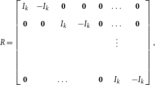 \begin{equation} R=\left[\begin{array}{c@{\quad}c@{\quad}c@{\quad}c@{\quad}c@{\quad}c@{\quad}c} I_k & -I_k & \mathbf{0} & \mathbf{0} & \mathbf{0} & \dots &\mathbf{0}\\[5pt] \mathbf{0} & \mathbf{0} & I_k & -I_k & \mathbf{0} &\dots &\mathbf{0}\\[5pt] & & & & &\vdots &\\[5pt] & & & & &&\\[5pt] \mathbf{0} & & \dots & & \mathbf{0}& I_k & -I_k \end{array}\right], \end{equation}
and $p=Nk$
.
$p=Nk$
.
3.1.1. Asymptotic results for the Stein-like shrinkage estimator
Our analysis is asymptotic as the time series dimension $T \rightarrow \infty$
while the number of individual units,
$T \rightarrow \infty$
while the number of individual units, $N$
, is fixed. Under the local alternative assumption, consider the parameter sequences of the form
$N$
, is fixed. Under the local alternative assumption, consider the parameter sequences of the form
 \begin{equation} \boldsymbol{{b}}=\boldsymbol{{b}}_0+\frac{\boldsymbol{{h}}}{\sqrt{T}}, \end{equation}
where $\boldsymbol{{b}}$
is the true parameter value,
$\boldsymbol{{b}}$
is the true parameter value, $\boldsymbol{{b}}_0$
is the slope coefficients under the assumption of no break (
$\boldsymbol{{b}}_0$
is the slope coefficients under the assumption of no break ( $\beta _{i(1)}=\beta _{i(2)}$
, for
$\beta _{i(1)}=\beta _{i(2)}$
, for $i=1, \dots N$
), and
$i=1, \dots N$
), and $\boldsymbol{{h}}$
shows the magnitude of the break size in the coefficients. Thus, for any fixed
$\boldsymbol{{h}}$
shows the magnitude of the break size in the coefficients. Thus, for any fixed $\boldsymbol{{h}}$
, the break size
$\boldsymbol{{h}}$
, the break size $\boldsymbol{{h}}/\sqrt{T}$
converges to zero as the sample size increases. We allow the size of the break to be different across individuals. That means that for each individual
$\boldsymbol{{h}}/\sqrt{T}$
converges to zero as the sample size increases. We allow the size of the break to be different across individuals. That means that for each individual $i=1, \dots, N$
, we have
$i=1, \dots, N$
, we have $\beta _{i(1)}=\beta _{i(2)}+ \frac{\delta _i}{\sqrt{T}}$
, or generally
$\beta _{i(1)}=\beta _{i(2)}+ \frac{\delta _i}{\sqrt{T}}$
, or generally
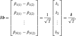 \begin{equation} R\boldsymbol{{b}}= \begin{bmatrix} \beta _{1(1)}-\beta _{1(2)} \\[5pt] \beta _{2(1)}-\beta _{2(2)} \\[5pt] \vdots \\[5pt] \beta _{N(1)}-\beta _{N(2)} \end{bmatrix}= \frac{1}{\sqrt{T}} \begin{bmatrix} \delta _1 \\[5pt] \delta _2 \\[5pt] \vdots \\[5pt] \delta _N \end{bmatrix} = \frac{\boldsymbol{\delta }}{\sqrt{T}}, \end{equation}
where $\boldsymbol{\delta }= (\delta'_{\!\!1}, \dots, \delta'_{\!\!N})'$
is a vector of
$\boldsymbol{\delta }= (\delta'_{\!\!1}, \dots, \delta'_{\!\!N})'$
is a vector of $Nk \times 1$
, and the restriction matrix
$Nk \times 1$
, and the restriction matrix $R$
is defined in (12). We note that
$R$
is defined in (12). We note that $R\boldsymbol{{h}}=\boldsymbol{\delta }$
, and
$R\boldsymbol{{h}}=\boldsymbol{\delta }$
, and $R\boldsymbol{{b}}_0=\textbf{0}$
under the assumption of no break. In the following theorem, we derive the asymptotic distributions of the unrestricted estimator, restricted estimator, and the Stein-like shrinkage estimator.
$R\boldsymbol{{b}}_0=\textbf{0}$
under the assumption of no break. In the following theorem, we derive the asymptotic distributions of the unrestricted estimator, restricted estimator, and the Stein-like shrinkage estimator.
THEOREM 1. Under Assumptions 1– 3 , along the sequences ( 13 ), the asymptotic distribution of the unrestricted estimator is
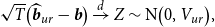 \begin{equation} \begin{aligned} \sqrt{T} \big ( \widehat{\boldsymbol{{b}}}_{ur}-\boldsymbol{{b}} \big ) \xrightarrow{d} Z \sim \text{N} \big (0, V_{ur} \big ),\\[5pt] \end{aligned} \end{equation}
where $V_{ur}=\Big ({\mathbb{E}} \big ( \frac{X'{\Omega }^{-1} X}{T}\big )\Big )^{-1}$
is the variance of the unrestricted estimator, and the asymptotic distribution of the restricted estimator is
$V_{ur}=\Big ({\mathbb{E}} \big ( \frac{X'{\Omega }^{-1} X}{T}\big )\Big )^{-1}$
is the variance of the unrestricted estimator, and the asymptotic distribution of the restricted estimator is
 \begin{equation} \sqrt{T} \big ( \widehat{\boldsymbol{{b}}}_{r}-\boldsymbol{{b}} \big ) \xrightarrow{d} Z-V_{ur} R' \big (R V_{ur} R' \big )^{-1} R (Z+\boldsymbol{{h}}). \end{equation}
In addition, the asymptotic distribution of the loss function, the weight, and the Stein-like shrinkage estimator is
 \begin{equation} D_T= T(\widehat{\boldsymbol{{b}}}_{ur}- \widehat{\boldsymbol{{b}}}_r)'{\mathbb{W}} (\widehat{\boldsymbol{{b}}}_{ur}- \widehat{\boldsymbol{{b}}}_r) \xrightarrow{d} (Z+\boldsymbol{{h}})' B (Z+\boldsymbol{{h}}), \end{equation}
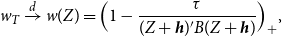 \begin{equation} w_T \xrightarrow{d} w(Z) = \Big (1- \frac{\tau }{(Z+\boldsymbol{{h}})' B (Z+\boldsymbol{{h}})} \Big )_+, \end{equation}
 \begin{align} \sqrt{T} \big (\widehat{\boldsymbol{{b}}}_w-\boldsymbol{{b}} \big ) \xrightarrow{d} Z-w(Z) V_{ur} R' \Big [RV_{ur} R' \Big ]^{-1} R (Z+\boldsymbol{{h}}), \end{align}
where $B \equiv R' \Big [R V_{ur} R' \Big ]^{-1} R V_{ur}{\mathbb{W}} V_{ur} R' \ \Big [R \ V_{ur} R' \Big ]^{-1} R$
is a
$B \equiv R' \Big [R V_{ur} R' \Big ]^{-1} R V_{ur}{\mathbb{W}} V_{ur} R' \ \Big [R \ V_{ur} R' \Big ]^{-1} R$
is a $2Nk \times 2Nk$
matrix.
$2Nk \times 2Nk$
matrix.
See Appendix A.1 for the proof of this theorem. Theorem 1 shows that the asymptotic distribution of the Stein-like shrinkage estimator is a nonlinear function of the normal random vector $Z$
and the non-centrality parameter
$Z$
and the non-centrality parameter $\boldsymbol{{h}}$
.
$\boldsymbol{{h}}$
.
REMARK 1. Lee et al. (Reference Lee, Parsaeian and Ullah2022a) consider a univariate time series model with a focus on forecasting. In this paper, we consider a SUR model and focus on improving the estimation of the slope coefficients within each regime and also improving forecasts utilizing the improved estimator of the slope coefficients. The theoretical derivations of asymptotic distributions of the estimators provided in Theorem 1 (and subsequent theorems) are significantly different from those of Lee et al. (Reference Lee, Parsaeian and Ullah2022a) due to differences in the models. Besides, the restricted estimator considered in this paper is general which can be obtained using different linear restrictions on the model parameters. For example, under two breaks, it may be the case that slope coefficients in the first and third regimes are equal while different with the second regime. Another restriction would be to allow for partial changes in the slope coefficients, or if one is interested to shrink part of the slope coefficients.
When an estimator has an asymptotic distribution, $\sqrt{T}(\widehat{\beta }-\beta ) \xrightarrow{d} \varpi$
, we define its asymptotic risk as
$\sqrt{T}(\widehat{\beta }-\beta ) \xrightarrow{d} \varpi$
, we define its asymptotic risk as $\rho (\widehat{\beta },{\mathbb{W}})={\mathbb{E}}(\varpi '{\mathbb{W}} \varpi )$
. See Lehmann and Casella (Reference Lehmann and Casella1998). Using Theorem 1, we derive the asymptotic risk for the Stein-like shrinkage estimator. Theorem 2 provides the result.
$\rho (\widehat{\beta },{\mathbb{W}})={\mathbb{E}}(\varpi '{\mathbb{W}} \varpi )$
. See Lehmann and Casella (Reference Lehmann and Casella1998). Using Theorem 1, we derive the asymptotic risk for the Stein-like shrinkage estimator. Theorem 2 provides the result.
THEOREM 2.
Under Assumptions
1–
3
, for $0 \lt \tau \leq 2 (Nk- 2)$
, and for
$0 \lt \tau \leq 2 (Nk- 2)$
, and for ${\mathbb{W}}=V_{ur}^{-1}$
, the asymptotic risk for the Stein-like shrinkage estimator is
${\mathbb{W}}=V_{ur}^{-1}$
, the asymptotic risk for the Stein-like shrinkage estimator is
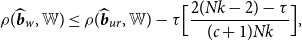 \begin{equation} \begin{aligned} \rho (\widehat{\boldsymbol{{b}}}_w,{\mathbb{W}}) \leq \rho (\widehat{\boldsymbol{{b}}}_{ur},{\mathbb{W}})- \tau \Big [ \frac{2 (Nk- 2) -\tau }{ (c+1) Nk}\Big ], \end{aligned} \end{equation}
where $0 \lt c \lt \infty$
.
$0 \lt c \lt \infty$
.
See Appendix A.2 for the proof of this theorem.Footnote
4
Theorem 2 shows that the asymptotic risk of the Stein-like shrinkage estimator is smaller than that of the unrestricted estimator. As the shrinkage parameter, $\tau$
, is unknown, we find it by minimizing the asymptotic risk. Theorem 3 shows the optimal value of the shrinkage parameter, denoted by
$\tau$
, is unknown, we find it by minimizing the asymptotic risk. Theorem 3 shows the optimal value of the shrinkage parameter, denoted by $\tau ^*_{opt}$
, and the associated asymptotic risk for the Stein-like shrinkage estimator.
$\tau ^*_{opt}$
, and the associated asymptotic risk for the Stein-like shrinkage estimator.
THEOREM 3.
When ${\mathbb{W}}= V_{ur}^{-1}$
and
${\mathbb{W}}= V_{ur}^{-1}$
and $Nk\gt 2$
, the optimal value of
$Nk\gt 2$
, the optimal value of $\tau$
is
$\tau$
is
 \begin{equation} \tau ^*_{opt}=Nk- 2, \end{equation}
where $\tau ^*_{opt}$
is positive as long as
$\tau ^*_{opt}$
is positive as long as $Nk\gt 2$
. Also, the asymptotic risk for the Stein-like shrinkage estimator after plugging the
$Nk\gt 2$
. Also, the asymptotic risk for the Stein-like shrinkage estimator after plugging the $\tau ^*_{opt}$
is
$\tau ^*_{opt}$
is
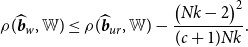 \begin{equation} \rho (\widehat{\boldsymbol{{b}}}_w,{\mathbb{W}}) \leq \rho (\widehat{\boldsymbol{{b}}}_{ur},{\mathbb{W}})- \frac{\big ( Nk- 2 \big )^2}{(c+1)Nk}. \end{equation}
Theorem 3 shows that the asymptotic risk of the Stein-like shrinkage estimator is smaller than that of the unrestricted estimator as long as $Nk\gt 2$
. Besides, the out-performance of the Stein-like shrinkage estimator over the unrestricted estimator will increase for small break sizes, large number of individuals, or large number of regressors.
$Nk\gt 2$
. Besides, the out-performance of the Stein-like shrinkage estimator over the unrestricted estimator will increase for small break sizes, large number of individuals, or large number of regressors.
3.2. Minimal MSE estimator
As an alternative to the shrinkage weight, we consider a weight between zero and one. Therefore, our second proposed estimator, the minimal MSE estimator, is
 \begin{equation} \widehat{\boldsymbol{{b}}}_{\gamma } ={\gamma } \widehat{\boldsymbol{{b}}}_{r}+ (1-\gamma ) \widehat{\boldsymbol{{b}}}_{ur}, \quad \gamma \in [0 \ 1] \end{equation}
where $\widehat{\boldsymbol{{b}}}_{ur}$
and
$\widehat{\boldsymbol{{b}}}_{ur}$
and $\widehat{\boldsymbol{{b}}}_{r}$
are defined in (10) and (11), respectively. Using the asymptotic distribution of the estimators in (15) and (16), we derive the asymptotic risk for the minimal MSE estimator as
$\widehat{\boldsymbol{{b}}}_{r}$
are defined in (10) and (11), respectively. Using the asymptotic distribution of the estimators in (15) and (16), we derive the asymptotic risk for the minimal MSE estimator as
 \begin{equation} \rho (\widehat{\boldsymbol{{b}}}_\gamma,{\mathbb{W}})= \rho (\widehat{\boldsymbol{{b}}}_{ur},{\mathbb{W}})+ \gamma ^2 \big (\boldsymbol{{h}}' B \boldsymbol{{h}}+ Nk \big ) -2 \gamma \ Nk. \end{equation}
By minimizing the asymptotic risk with respect to $\gamma$
in (24), the optimal value of the weight denoted by
$\gamma$
in (24), the optimal value of the weight denoted by $\gamma ^*_{opt}$
is
$\gamma ^*_{opt}$
is
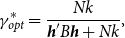 \begin{equation} \gamma ^*_{opt}=\frac{Nk}{\boldsymbol{{h}}' B \boldsymbol{{h}}+Nk}, \end{equation}
which by plugging the unbiased estimator of its denominator we have
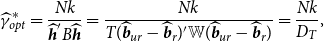 \begin{equation} \begin{aligned} \widehat{\gamma }^*_{opt}=\frac{Nk}{\widehat{\boldsymbol{{h}}}' B \widehat{\boldsymbol{{h}}}} & =\frac{Nk}{T(\widehat{\boldsymbol{{b}}}_{ur}- \widehat{\boldsymbol{{b}}}_r)'{\mathbb{W}} (\widehat{\boldsymbol{{b}}}_{ur}- \widehat{\boldsymbol{{b}}}_r)}= \frac{Nk}{D_T}, \end{aligned} \end{equation}
where the second equality holds noting that $V_{ur} R' \Big [R V_{ur} R' \Big ]^{-1} R (\widehat{\boldsymbol{{b}}}_{ur}- \widehat{\boldsymbol{{b}}}_r)=(\widehat{\boldsymbol{{b}}}_{ur}- \widehat{\boldsymbol{{b}}}_r)$
. Hence,
$V_{ur} R' \Big [R V_{ur} R' \Big ]^{-1} R (\widehat{\boldsymbol{{b}}}_{ur}- \widehat{\boldsymbol{{b}}}_r)=(\widehat{\boldsymbol{{b}}}_{ur}- \widehat{\boldsymbol{{b}}}_r)$
. Hence, $T(\widehat{\boldsymbol{{b}}}_{ur}- \widehat{\boldsymbol{{b}}}_r)' B (\widehat{\boldsymbol{{b}}}_{ur}- \widehat{\boldsymbol{{b}}}_r)=T(\widehat{\boldsymbol{{b}}}_{ur}- \widehat{\boldsymbol{{b}}}_r)'{\mathbb{W}} (\widehat{\boldsymbol{{b}}}_{ur}- \widehat{\boldsymbol{{b}}}_r)$
.Footnote
5
$T(\widehat{\boldsymbol{{b}}}_{ur}- \widehat{\boldsymbol{{b}}}_r)' B (\widehat{\boldsymbol{{b}}}_{ur}- \widehat{\boldsymbol{{b}}}_r)=T(\widehat{\boldsymbol{{b}}}_{ur}- \widehat{\boldsymbol{{b}}}_r)'{\mathbb{W}} (\widehat{\boldsymbol{{b}}}_{ur}- \widehat{\boldsymbol{{b}}}_r)$
.Footnote
5
REMARK 2. By comparing $\widehat{\gamma }^*_{opt}$
in (26) and
$\widehat{\gamma }^*_{opt}$
in (26) and $\tau ^*_{opt}/D_T$
using (21), we see that the difference between the averaging weights of the Stein-like shrinkage estimator and the minimal MSE estimator is in their numerators. In other words, the optimal weight in (26) also depends on the distance between the restricted and unrestricted estimators. Basically, the idea behind the averaging estimator in (23) is similar to the Stein-like shrinkage estimator in (7). That is, when the difference between the restricted and unrestricted estimator is small, the minimal MSE estimator gives more weight to the restricted estimator, which is efficient under
$\tau ^*_{opt}/D_T$
using (21), we see that the difference between the averaging weights of the Stein-like shrinkage estimator and the minimal MSE estimator is in their numerators. In other words, the optimal weight in (26) also depends on the distance between the restricted and unrestricted estimators. Basically, the idea behind the averaging estimator in (23) is similar to the Stein-like shrinkage estimator in (7). That is, when the difference between the restricted and unrestricted estimator is small, the minimal MSE estimator gives more weight to the restricted estimator, which is efficient under $R \boldsymbol{{b}}=\textbf{0}$
, and the opposite is true for the large distance between the two estimators. Therefore, the proposed averaging estimator in (23) is also a Stein-like shrinkage estimator that incorporates the trade-off between the bias and variance efficiency.
$R \boldsymbol{{b}}=\textbf{0}$
, and the opposite is true for the large distance between the two estimators. Therefore, the proposed averaging estimator in (23) is also a Stein-like shrinkage estimator that incorporates the trade-off between the bias and variance efficiency.
Given the optimal weight in (26), we derive the asymptotic risk for the minimal MSE estimator. Theorem 4 presents the results.
THEOREM 4.
Under Assumptions
1–
3
, and given the optimal value of the weight in (
26
), for ${\mathbb{W}}=V_{ur}^{-1}$
, the asymptotic risk of the minimal MSE is
${\mathbb{W}}=V_{ur}^{-1}$
, the asymptotic risk of the minimal MSE is
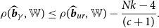 \begin{equation} \rho (\widehat{\boldsymbol{{b}}}_\gamma,{\mathbb{W}}) \leq \rho (\widehat{\boldsymbol{{b}}}_{ur},{\mathbb{W}})- \frac{Nk-4}{(c+1)}. \end{equation}
See Appendix A.4 for the proof of this theorem.Footnote
6
Theorem 4 shows that the asymptotic risk of the minimal MSE estimator is smaller than that of the unrestricted estimator as long as $Nk\gt 4$
.
$Nk\gt 4$
.
REMARK 3. Examining the results of Theorems 3 and 4, we find that the necessary condition for the out-performance of the Stein-like shrinkage estimator over the unrestricted estimator is $Nk\gt 2$
, while the condition is
$Nk\gt 2$
, while the condition is $Nk\gt 4$
for the minimal MSE estimator, which is slightly a stronger condition. Furthermore, the difference between their risks, for
$Nk\gt 4$
for the minimal MSE estimator, which is slightly a stronger condition. Furthermore, the difference between their risks, for ${\mathbb{W}}= V_{ur}^{-1}$
, is
${\mathbb{W}}= V_{ur}^{-1}$
, is
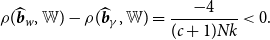 \begin{equation} \rho (\widehat{\boldsymbol{{b}}}_w,{\mathbb{W}})- \rho (\widehat{\boldsymbol{{b}}}_\gamma,{\mathbb{W}})= \frac{-4}{(c+1) Nk}\lt 0. \end{equation}
Therefore, the Stein-like shrinkage estimator has a smaller asymptotic risk than the minimal MSE estimator. In addition, for small break sizes, we expect to see a better performance for the Stein-like shrinkage estimator relative to the minimal MSE estimator, in the sense of a smaller asymptotic risk. For a large break size, a large number of regressors, or a large number of individuals, we expect to see an equal performance between them.Footnote 7
3.3. Forecasting under structural breaks
Generating accurate forecasts in the presence of structural breaks requires careful consideration of bias-variance trade-off. Our introduced Stein-like shrinkage estimator and the minimal MSE estimator consider the bias-variance trade-off in the estimation of parameters and can thus be used to generate forecasts. As the true parameters that enter the forecasting period are the coefficients in the post-break sample, we define a $Nk \times 2Nk$
selection matrix
$Nk \times 2Nk$
selection matrix $G$
such that
$G$
such that
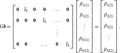 \begin{equation} G\boldsymbol{{b}}= \left[\begin{array}{c@{\quad}c@{\quad}c@{\quad}c@{\quad}c@{\quad}c} \mathbf{0} & I_k & \mathbf{0} & \mathbf{0} & \dots & \mathbf{0} \\[5pt] \mathbf{0} &\mathbf{0} & \mathbf{0} & I_k & \dots & \mathbf{0} \\[5pt] & & & &\vdots &\\[5pt] \mathbf{0} &\mathbf{0} & & \dots & \mathbf{0} & I_k \end{array}\right] \begin{bmatrix} \beta _{1(1)} \\[5pt] \beta _{1(2)} \\[5pt] \vdots \\[5pt] \beta _{N(1)} \\[5pt] \beta _{N(2)} \end{bmatrix} = \begin{bmatrix} \beta _{1(2)} \\[5pt] \beta _{2(2)} \\[5pt] \beta _{3(2)} \\[5pt] \vdots \\[5pt] \beta _{N(2)} \end{bmatrix}. \end{equation}
By multiplying $G$
to the Stein-like shrinkage estimator, we have
$G$
to the Stein-like shrinkage estimator, we have
 \begin{equation} G\widehat{\boldsymbol{{b}}}_w= w_T G\widehat{\boldsymbol{{b}}}_{ur}+ (1-w_T) G \widehat{\boldsymbol{{b}}}_{r}, \end{equation}
where $G\widehat{\boldsymbol{{b}}}_{ur}$
estimates the coefficients only by using the observations after the break point (also known as the post-break estimator), and
$G\widehat{\boldsymbol{{b}}}_{ur}$
estimates the coefficients only by using the observations after the break point (also known as the post-break estimator), and $ G \widehat{\boldsymbol{{b}}}_{r}$
is the restricted estimator under the assumption of no break in the model. The assumption of no break lines up with the fact that, with a small break, ignoring the break and estimating the coefficients using full-sample observations would result in a better forecast (lower MSFE), see Boot and Pick (Reference Boot and Pick2020).
$ G \widehat{\boldsymbol{{b}}}_{r}$
is the restricted estimator under the assumption of no break in the model. The assumption of no break lines up with the fact that, with a small break, ignoring the break and estimating the coefficients using full-sample observations would result in a better forecast (lower MSFE), see Boot and Pick (Reference Boot and Pick2020).
Define the MSFE of the Stein-like shrinkage estimator as
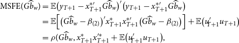 \begin{equation} \begin{aligned} \text{MSFE}(G \widehat{b}_w)&= {\mathbb{E}} \big ( y_{T+1}-x_{T+1}^{*\prime} G\widehat{b}_w \big )'\big ( y_{T+1}-x_{T+1}^{*\prime} G\widehat{b}_w \big ) \\&={\mathbb{E}} \Big [ \big (G\widehat{b}_w-\beta _{(2)}\big )' x_{T+1}^* x_{T+1}^{*\prime} \big (G\widehat{b}_w-\beta _{(2)}\big ) \Big ]+{\mathbb{E}} \big (u'_{\!\!T+1} u_{T+1} \big )\\&= \rho (G \widehat{b}_w, x_{T+1}^*x^{\prime*}_{T+1}+{\mathbb{E}} \big (u'_{\!\!T+1} u_{T+1} \big ) , \end{aligned} \end{equation}
where $y_{T+1}=(y_{1,T+1}, \dots, y_{N,T+1})'$
is an
$y_{T+1}=(y_{1,T+1}, \dots, y_{N,T+1})'$
is an $N \times 1$
vector of dependent variables at time
$N \times 1$
vector of dependent variables at time $T+1$
,
$T+1$
, $x_{T+1}^*=\text{diag}(x_{1,T+1}, \dots, x_{N,T+1})$
is an
$x_{T+1}^*=\text{diag}(x_{1,T+1}, \dots, x_{N,T+1})$
is an $Nk \times N$
matrix of regressors,
$Nk \times N$
matrix of regressors, $\beta _{(2)}=(\beta '_{\!\!1(2)}, \dots, \beta '_{\!\!N(2)})'$
, and
$\beta _{(2)}=(\beta '_{\!\!1(2)}, \dots, \beta '_{\!\!N(2)})'$
, and $u_{T+1}=(u_{1,T+1}, \dots, u_{N,T+1})'$
. Thus, by choosing
$u_{T+1}=(u_{1,T+1}, \dots, u_{N,T+1})'$
. Thus, by choosing $\mathbb{W}$
accordingly, we use the asymptotic risk,
$\mathbb{W}$
accordingly, we use the asymptotic risk, $\rho (G \widehat{b}_w,{\mathbb{W}})$
, to approximate the first term on the right-hand side of the MSFE. This along with
$\rho (G \widehat{b}_w,{\mathbb{W}})$
, to approximate the first term on the right-hand side of the MSFE. This along with ${\mathbb{E}} \big (u'_{\!\!T+1} u_{T+1} \big )$
corresponds to the one-step-ahead MSFE. As the second term in (31),
${\mathbb{E}} \big (u'_{\!\!T+1} u_{T+1} \big )$
corresponds to the one-step-ahead MSFE. As the second term in (31), ${\mathbb{E}} \big (u'_{\!\!T+1}u_{T+1} \big )$
, does not depend on
${\mathbb{E}} \big (u'_{\!\!T+1}u_{T+1} \big )$
, does not depend on $\tau$
, minimizing the MSFE is equivalent to minimizing the asymptotic risk. Similarly, we define the MSFE for the minimal MSE estimator. Theorem 5 summarizes the results of MSFE for the estimators.
$\tau$
, minimizing the MSFE is equivalent to minimizing the asymptotic risk. Similarly, we define the MSFE for the minimal MSE estimator. Theorem 5 summarizes the results of MSFE for the estimators.
THEOREM 5. Under Assumptions 1– 3 , the MSFEs of the Stein-like shrinkage estimator is
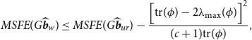 \begin{equation} \begin{aligned} MSFE(G\widehat{\boldsymbol{{b}}}_w) & \leq MSFE(G\widehat{\boldsymbol{{b}}}_{ur})- \frac{\Big [ \textrm{tr}(\phi )- 2\lambda _{\textrm{max}}(\phi ) \Big ]^2}{(c+1) \textrm{tr} (\phi )}, \end{aligned} \end{equation}
and the MSFE of the minimal MSEs estimator is
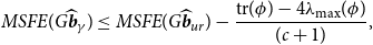 \begin{equation} \begin{aligned} MSFE(G\widehat{\boldsymbol{{b}}}_\gamma ) & \leq MSFE(G\widehat{\boldsymbol{{b}}}_{ur})- \frac{ \textrm{tr}(\phi )- 4\lambda _{\textrm{max}}(\phi )}{(c+1) }, \end{aligned} \end{equation}
where $\phi \equiv{\mathbb{W}}^{1/2} G V_{ur} R' \Big [R V_{ur} R' \Big ]^{-1} R V_{ur} G'{\mathbb{W}}^{1/2}$
, and
$\phi \equiv{\mathbb{W}}^{1/2} G V_{ur} R' \Big [R V_{ur} R' \Big ]^{-1} R V_{ur} G'{\mathbb{W}}^{1/2}$
, and ${\mathbb{W}}=x_{T+1}^* x_{T+1}^{*\prime}$
.
${\mathbb{W}}=x_{T+1}^* x_{T+1}^{*\prime}$
.
Theorem 5 shows that the MSFE of the Stein-like shrinkage estimator is smaller than that of the unrestricted estimator when $d=\frac{\text{tr}(\phi )}{\text{max}(\phi )}\gt 2$
, whereas the similar condition for the minimal MSE estimator is
$d=\frac{\text{tr}(\phi )}{\text{max}(\phi )}\gt 2$
, whereas the similar condition for the minimal MSE estimator is $d\gt 4$
.
$d\gt 4$
.
REMARK 4. The proposed Stein-like shrinkage estimator can be generalized to account for the possibility of multiple common breaks. Similar to the single break case, the unrestricted estimator uses the observations within each regime separately, and the restricted estimator uses the full sample of observations. In case of forecasting, the shrinkage estimator is the weighted average of the restricted estimator and the unrestricted estimator using the observations after the most recent break point.Footnote 8
4. Monte Carlo simulations
This section employs Monte Carlo simulations to examine the performance of the theoretical results obtained in this paper. To do this, we consider the following data generating process:
 \begin{equation} y_{i,t}= \begin{cases} x'_{\!\!i,t} \beta _{i(1)}+ u_{i,t} \quad \text{for} \ i=1, \dots, N, \quad t=1, \dots, T_1,\\[5pt] x'_{\!\!i,t} \beta _{i(2)}+ u_{i,t} \quad \text{for} \ i=1, \dots, N, \quad t=T_1+1, \dots, T, \end{cases} \end{equation}
where $x_{i,t} \sim \text{N}(0,1)$
, and we set the first column of that to be a vector of ones in order to allow for the fixed effect. Let the time series dimension be
$x_{i,t} \sim \text{N}(0,1)$
, and we set the first column of that to be a vector of ones in order to allow for the fixed effect. Let the time series dimension be $T=100$
, the number of individual units be
$T=100$
, the number of individual units be $N=5$
, and
$N=5$
, and $k \in \{1, 3\}$
. We consider different values for true break points, which are proportional to the sample size,
$k \in \{1, 3\}$
. We consider different values for true break points, which are proportional to the sample size, $b_1 \equiv \frac{T_1}{T} \in \{0.2, 0.8\}$
.Footnote
9
$b_1 \equiv \frac{T_1}{T} \in \{0.2, 0.8\}$
.Footnote
9
Let $\beta _{i(2)}$
be a vector of ones, and
$\beta _{i(2)}$
be a vector of ones, and $\delta _i= \beta _{i(1)}-\beta _{i(2)}= \frac{i}{N-1}\times s$
shows the true break size in the coefficients, where
$\delta _i= \beta _{i(1)}-\beta _{i(2)}= \frac{i}{N-1}\times s$
shows the true break size in the coefficients, where $s$
varies from
$s$
varies from $0$
to
$0$
to $1$
in increments of
$1$
in increments of $0.1$
. Moreover, define
$0.1$
. Moreover, define $\xi _{1(1)} \sim \text{N} \big (0,\sigma _{(1)}^2 \big )$
and
$\xi _{1(1)} \sim \text{N} \big (0,\sigma _{(1)}^2 \big )$
and $\xi _{1(2)} \sim \text{N}\big (0,\sigma _{(2)}^2 \big )$
, and let
$\xi _{1(2)} \sim \text{N}\big (0,\sigma _{(2)}^2 \big )$
, and let $q \equiv \sigma _{(1)}/ \sigma _{(2)}$
with
$q \equiv \sigma _{(1)}/ \sigma _{(2)}$
with $q \in \{ 0.5, 1, 2\}$
. To allow for the cross-sectional dependence, we consider
$q \in \{ 0.5, 1, 2\}$
. To allow for the cross-sectional dependence, we consider
 \begin{equation} \begin{cases} \begin{aligned} u_{i(1)}&=0.5\xi _{1(1)}+ v_{i(1)} \quad \text{for} \quad i=1, \dots, N, \quad t=1, \dots, T_1\\[5pt] u_{i(2)}&=0.5\xi _{1(2)}+ v_{i(2)} \quad \text{for} \quad i=1, \dots, N, \quad t=T_1+1, \dots, T, \end{aligned} \end{cases} \end{equation}
where $v_{i(1)} \sim \text{N}(0, \sqrt{i} \ \sigma _{(1)}^2)$
, and
$v_{i(1)} \sim \text{N}(0, \sqrt{i} \ \sigma _{(1)}^2)$
, and $v_{i(2)} \sim \text{N}(0, \sqrt{i} \ \sigma _{(2)}^2)$
. As the break point, break sizes in the slope coefficients and the error variances are unknown in practice, we estimate them to incorporate the uncertainty regarding the estimation of these parameters in our analysis. The break point is estimated using the method proposed by Qu and Perron (Reference Qu and Perron2007).
$v_{i(2)} \sim \text{N}(0, \sqrt{i} \ \sigma _{(2)}^2)$
. As the break point, break sizes in the slope coefficients and the error variances are unknown in practice, we estimate them to incorporate the uncertainty regarding the estimation of these parameters in our analysis. The break point is estimated using the method proposed by Qu and Perron (Reference Qu and Perron2007).
In this study, we compare the performance of the Stein-like shrinkage estimator, the minimal MSE estimator, the unrestricted estimator, and the pretest estimator. We calculate the pretest estimator, denoted by $\widehat{\boldsymbol{{b}}}_{\text{PT}}$
, as
$\widehat{\boldsymbol{{b}}}_{\text{PT}}$
, as
 \begin{equation} \widehat{\boldsymbol{{b}}}_{\text{PT}}= \widehat{\boldsymbol{{b}}}_r \ \text{I}(D_T \lt c_v)+\widehat{\boldsymbol{{b}}}_{ur} \ \text{I}(D_T \geq c_v), \end{equation}
where $c_v$
is the
$c_v$
is the $5\%$
critical value from the chi-square distribution, and
$5\%$
critical value from the chi-square distribution, and $D_T$
is the Wald-type test statistic in (9). Thus, the pretest estimator selects a restricted estimator when the Wald statistic is insignificant and selects the unrestricted estimator when the Wald statistic is significant. We report the relative MSE and set the unrestricted estimator as the benchmark estimator so that the relative MSE of the unrestricted estimator is equal to one, that is, the relative MSEs are
$D_T$
is the Wald-type test statistic in (9). Thus, the pretest estimator selects a restricted estimator when the Wald statistic is insignificant and selects the unrestricted estimator when the Wald statistic is significant. We report the relative MSE and set the unrestricted estimator as the benchmark estimator so that the relative MSE of the unrestricted estimator is equal to one, that is, the relative MSEs are $\frac{\rho (\widehat{\boldsymbol{{b}}}_w,{\mathbb{W}})}{\rho (\widehat{\boldsymbol{{b}}}_{ur},{\mathbb{W}})}$
,
$\frac{\rho (\widehat{\boldsymbol{{b}}}_w,{\mathbb{W}})}{\rho (\widehat{\boldsymbol{{b}}}_{ur},{\mathbb{W}})}$
, $\frac{\rho (\widehat{\boldsymbol{{b}}}_\gamma,{\mathbb{W}})}{\rho (\widehat{\boldsymbol{{b}}}_{ur},{\mathbb{W}})}$ $\frac{\rho (\widehat{\boldsymbol{{b}}}_{\text{PT}},{\mathbb{W}})}{\rho (\widehat{\boldsymbol{{b}}}_{ur},{\mathbb{W}})}$
, and
$\frac{\rho (\widehat{\boldsymbol{{b}}}_{\text{PT}},{\mathbb{W}})}{\rho (\widehat{\boldsymbol{{b}}}_{ur},{\mathbb{W}})}$
, and $\frac{\rho (\widehat{\boldsymbol{{b}}}_{\text{ur}},{\mathbb{W}})}{\rho (\widehat{\boldsymbol{{b}}}_{ur},{\mathbb{W}})}$
. The relative MSE is a good measure for evaluating the estimation accuracy of different methods. In addition, it measures how different methods are compared with each others and what are the gains of methods relative to each other. Fig. 1 shows the results over 1000 Monte Carlo replications when
$\frac{\rho (\widehat{\boldsymbol{{b}}}_{\text{ur}},{\mathbb{W}})}{\rho (\widehat{\boldsymbol{{b}}}_{ur},{\mathbb{W}})}$
. The relative MSE is a good measure for evaluating the estimation accuracy of different methods. In addition, it measures how different methods are compared with each others and what are the gains of methods relative to each other. Fig. 1 shows the results over 1000 Monte Carlo replications when $N=5$
. Since we consider different break sizes for individuals, we show the proportion of the break size in the coefficients (
$N=5$
. Since we consider different break sizes for individuals, we show the proportion of the break size in the coefficients ( $s$
) in the horizontal axis. The vertical axis shows the relative MSE.
$s$
) in the horizontal axis. The vertical axis shows the relative MSE.
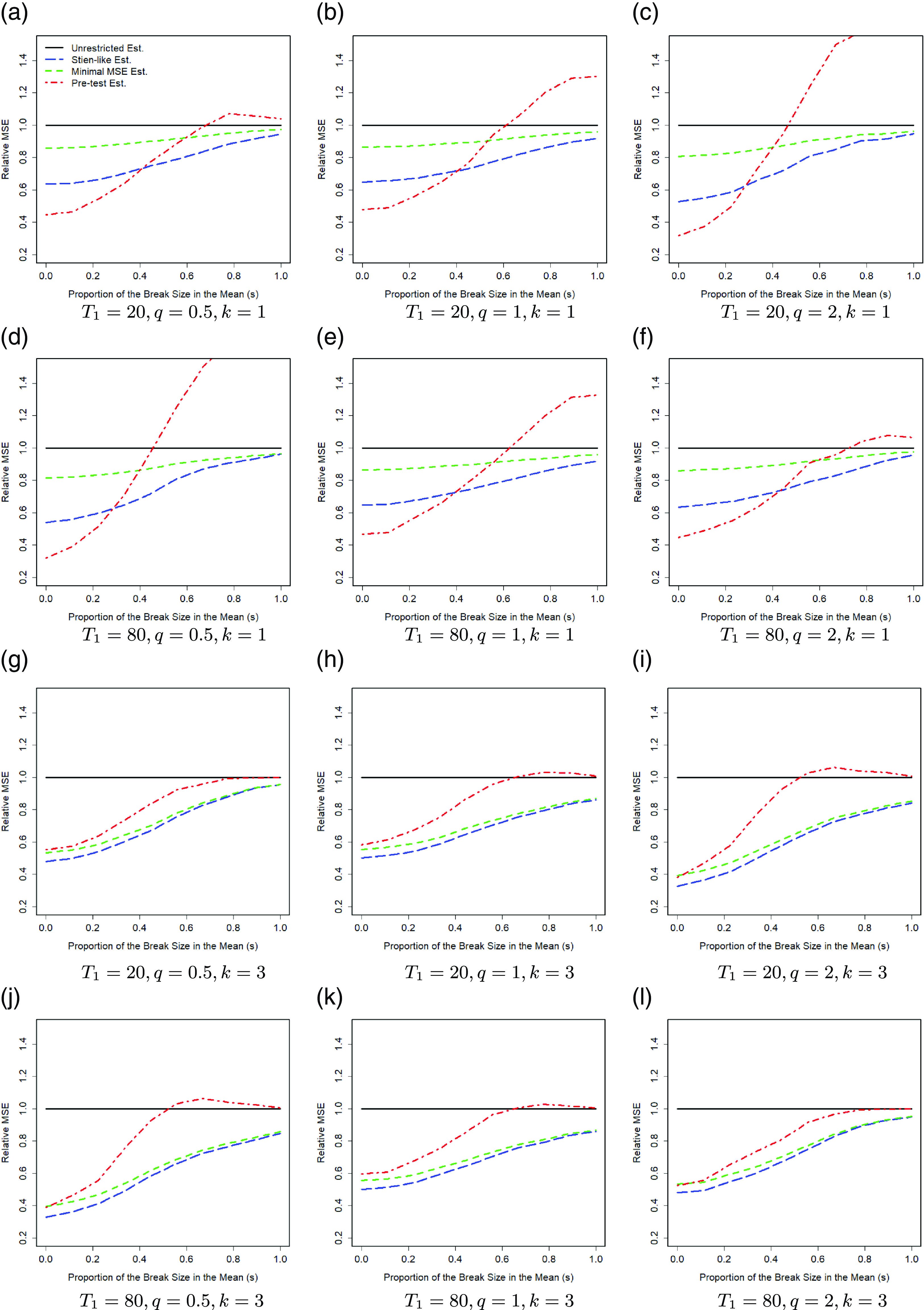
Figure 1. Monte Carlo results for $T=100$
,
$T=100$
, $N=5$
.
$N=5$
.
4.1. Simulation results
Based on the results of Fig. 1, the Stein-like shrinkage estimator has better performance than the unrestricted estimator, in the sense of having a smaller MSE, for any break sizes and break points. Fig. 1 shows the results with $k=1$
and
$k=1$
and $k=3$
. Based on Fig. 1, for the small-to-medium break sizes in the coefficients, the Stein-like shrinkage estimator performs much better than the unrestricted estimator. In this case, the shrinkage estimator assigns more weight to the restricted estimator to gain from its efficiency. As the break size in the coefficients increases, the Stein-like shrinkage estimator performs close to the unrestricted estimator, but still slightly better. This may be related to the large bias that the restricted estimator adds to the shrinkage estimator under large break sizes. Therefore, the shrinkage estimator assigns more weight to the unrestricted estimator and less weight to the restricted estimator. We note that even for the large break sizes, we still do not observe the under-performance of the Stein-like shrinkage estimator over the unrestricted estimator. When
$k=3$
. Based on Fig. 1, for the small-to-medium break sizes in the coefficients, the Stein-like shrinkage estimator performs much better than the unrestricted estimator. In this case, the shrinkage estimator assigns more weight to the restricted estimator to gain from its efficiency. As the break size in the coefficients increases, the Stein-like shrinkage estimator performs close to the unrestricted estimator, but still slightly better. This may be related to the large bias that the restricted estimator adds to the shrinkage estimator under large break sizes. Therefore, the shrinkage estimator assigns more weight to the unrestricted estimator and less weight to the restricted estimator. We note that even for the large break sizes, we still do not observe the under-performance of the Stein-like shrinkage estimator over the unrestricted estimator. When $q=0.5$
the error variance of the pre-break data is less than that of the post-break data while the opposite holds for
$q=0.5$
the error variance of the pre-break data is less than that of the post-break data while the opposite holds for $q=2$
. Looking at Fig. 1(a)–(c), we see the performance of the Stein-like shrinkage estimator is improving. When
$q=2$
. Looking at Fig. 1(a)–(c), we see the performance of the Stein-like shrinkage estimator is improving. When $q=0.5$
and
$q=0.5$
and $T_1 = 20$
, Fig. 1(a), the pre-break estimator performs poorly as it only has 20 observations. When we combine it with the restricted estimator, it cannot benefit significantly, as the post-break observations are more volatile (
$T_1 = 20$
, Fig. 1(a), the pre-break estimator performs poorly as it only has 20 observations. When we combine it with the restricted estimator, it cannot benefit significantly, as the post-break observations are more volatile ( $q = 0.5$
). However, for
$q = 0.5$
). However, for $q=2$
and
$q=2$
and $T_1=20$
, Fig. 1(c), when we combine the pre-break estimator with the restricted estimator, the estimator performs better, since the post-break observations are less volatile (
$T_1=20$
, Fig. 1(c), when we combine the pre-break estimator with the restricted estimator, the estimator performs better, since the post-break observations are less volatile ( $q = 2$
). For
$q = 2$
). For $T_1 =80$
and
$T_1 =80$
and $q = 0.5$
, Fig. 1(d), the post-break estimator performs poorly since it only has 20 observations. When we combine it with the restricted estimator, it benefits more compared to the previous case that
$q = 0.5$
, Fig. 1(d), the post-break estimator performs poorly since it only has 20 observations. When we combine it with the restricted estimator, it benefits more compared to the previous case that $T_1 = 20$
, because the pre-break observations are less volatile (
$T_1 = 20$
, because the pre-break observations are less volatile ( $q = 0.5$
). This pattern is observed for
$q = 0.5$
). This pattern is observed for $k=3$
as well. Besides, as we increase the number of regressors, the gain obtained from the Stein-like shrinkage estimator increases. In addition, the Stein-like shrinkage estimator performs better than the minimal MSE estimator for the small-to-medium break sizes in the coefficients. For large break sizes, these two estimators perform almost equally.
$k=3$
as well. Besides, as we increase the number of regressors, the gain obtained from the Stein-like shrinkage estimator increases. In addition, the Stein-like shrinkage estimator performs better than the minimal MSE estimator for the small-to-medium break sizes in the coefficients. For large break sizes, these two estimators perform almost equally.
All simulation results confirm the results of Theorems 3 and 4 that the performance of the Stein-like shrinkage estimator and the minimal MSE estimator are uniformly better than the unrestricted estimator in the sense of having lower MSE, for any break points, break sizes in the coefficients, and any $q$
. Generally, for large break sizes, large
$q$
. Generally, for large break sizes, large $N$
, or large number of regressors,
$N$
, or large number of regressors, $k$
, the shrinkage estimators have equal performance. This confirms our theoretical findings in Remark 3.
$k$
, the shrinkage estimators have equal performance. This confirms our theoretical findings in Remark 3.
The pretest estimator either uses the restricted estimator or the unrestricted estimator depending on the Wald test results. Generally, the MSE of the pretest estimator is similar to the restricted estimator for a small break size and is similar to the unrestricted estimator for a large break size, because these two extreme cases are better caught by the test statistic. For a moderate break size, however, the pretest estimator performs worse than the unrestricted estimator.
In order to see how the Stein-like shrinkage estimator assigns weights to the restricted and unrestricted estimators, we plot the estimated weights, $\widehat{w}_T$
, for the simulation results of Figs. 1(a) and (g). The estimated weights are shown in Fig. 2 in which the horizontal axis shows the break size in the mean, and the vertical axis shows the estimated Stein-like shrinkage weights. The results show that for small break sizes, the Stein-like shrinkage estimator mainly assigns a higher weight to the restricted estimator (estimated weight is small), while as the break size increases it assigns a larger weight to the unrestricted estimator (estimated weight is large). As the number of regressors increases, the range of the estimated weight becomes smaller. Similar patterns are seen under other specifications which are omitted to save space.
$\widehat{w}_T$
, for the simulation results of Figs. 1(a) and (g). The estimated weights are shown in Fig. 2 in which the horizontal axis shows the break size in the mean, and the vertical axis shows the estimated Stein-like shrinkage weights. The results show that for small break sizes, the Stein-like shrinkage estimator mainly assigns a higher weight to the restricted estimator (estimated weight is small), while as the break size increases it assigns a larger weight to the unrestricted estimator (estimated weight is large). As the number of regressors increases, the range of the estimated weight becomes smaller. Similar patterns are seen under other specifications which are omitted to save space.
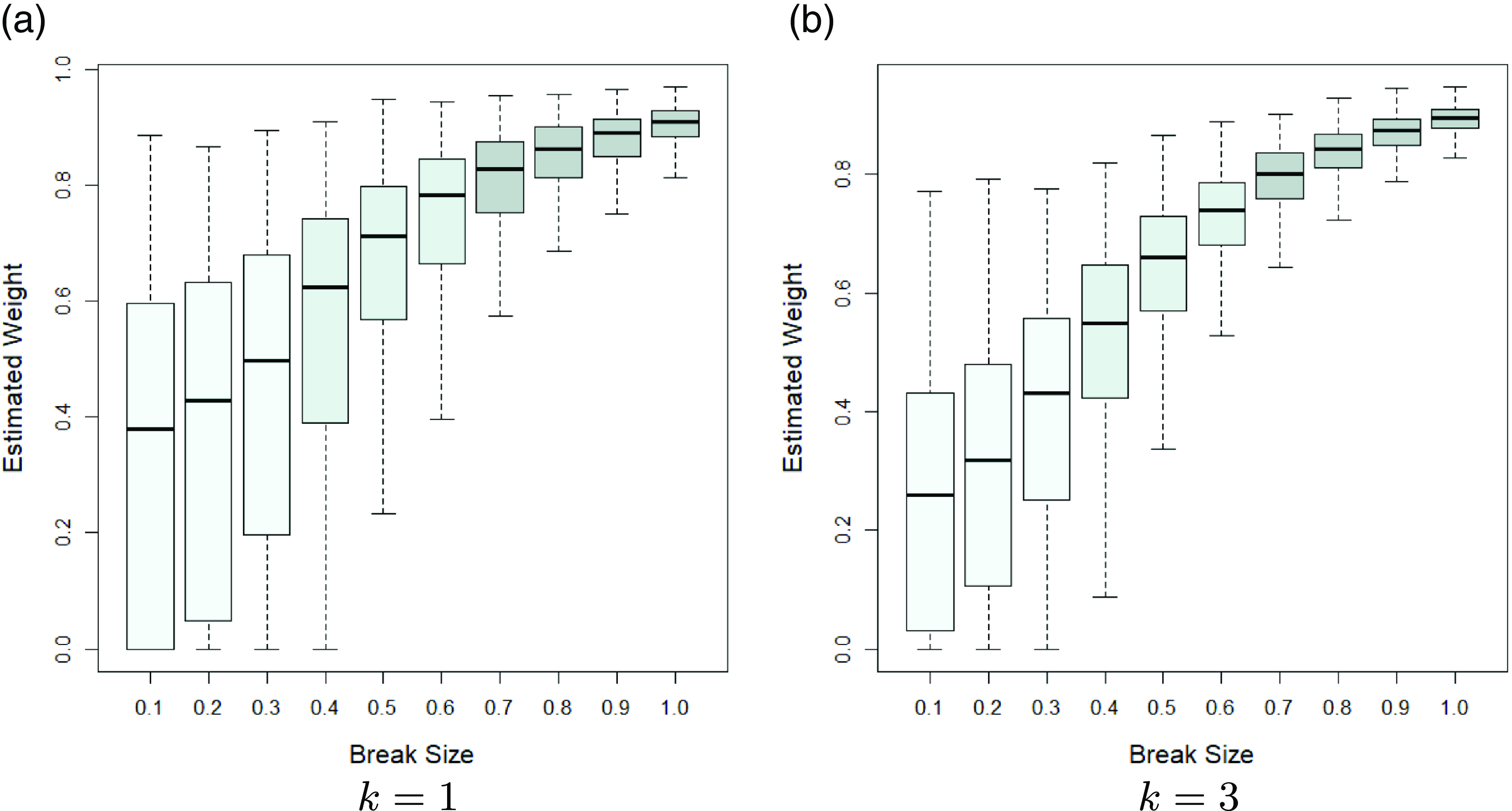
Figure 2. Boxplot for the estimated Stein-like shrinkage weight.
5. Empirical analysis
This section provides some empirical analysis for forecasting the growth rate of real output using a quarterly data set in G7 countries from 1995:Q1 to 2016:Q4.Footnote 10 The predictors for each country are the log real equity prices, the real short-term interest rate, and the difference between the long and short-term interest rates. The data are taken from the Global VAR (GVAR) dataset (2016 vintage). The data are available with the GVAR Toolbox, Mohaddes and Raissi (Reference Mohaddes and Raissi2018).
We evaluate the out-of-sample forecasting performance of the proposed Stein-like shrinkage estimator and the minimal MSE estimator with a range of alternative methods in terms of their MSFEs. The first two alternative methods are the SUR model that estimates the post-break slope coefficients across the entire cross-section (the unrestricted estimator) and the pretest estimator. We also consider some of the existing univariate time series forecasting approaches that provide forecasts independently in each cross-section series as alternative methods, that is, these time series methods ignore the cross-sectional dependence. These are the methods proposed by Pesaran et al. (Reference Pesaran, Pick and Pranovich2013) (labeled as “PPP” in tables), the five methods used in Pesaran and Timmermann (Reference Pesaran and Timmermann2007), namely, “Postbk,” “Troff,” “Pooled,” “WA,” “CV”, the full-sample forecast that ignores the break and uses the full-sample of observations (“Full”), the average window forecast proposed by Pesaran and Pick (Reference Pesaran and Pick2011) (“AveW”), the method proposed by Lee et al. (Reference Lee, Parsaeian and Ullah2022a) (“LPU”), and the forecast using the optimal window size proposed by Inoue et al. (Reference Inoue, Jin and Rossi2017) (“IJR”), which is designed for smoothly time-varying parameters.
We compute $h$
-step-ahead forecasts (
$h$
-step-ahead forecasts ( $h = 1, 2,3, 4$
) for different forecasting methods described above, using both rolling and expanding windows. The rolling window forecast is based on the most recent 10 years (40 quarters) of observations, the same window size used by Stock and Watson (Reference Stock and Watson2003). For the expanding window, we divide the sample of observations into two parts. The first
$h = 1, 2,3, 4$
) for different forecasting methods described above, using both rolling and expanding windows. The rolling window forecast is based on the most recent 10 years (40 quarters) of observations, the same window size used by Stock and Watson (Reference Stock and Watson2003). For the expanding window, we divide the sample of observations into two parts. The first $T$
observations are used as the initial in-sample estimation period, and the remaining observations are the pseudo out-of-sample evaluation period. The initial estimation period is from 1995:Q1 to 2004:Q4 (
$T$
observations are used as the initial in-sample estimation period, and the remaining observations are the pseudo out-of-sample evaluation period. The initial estimation period is from 1995:Q1 to 2004:Q4 ( $T=40$
), which leaves the out-of-sample period from 2005:Q1 to 2016:Q4. In both rolling and expanding window approaches, we initially estimate the break point using the Qu and Perron (Reference Qu and Perron2007) approach. Then, we generate
$T=40$
), which leaves the out-of-sample period from 2005:Q1 to 2016:Q4. In both rolling and expanding window approaches, we initially estimate the break point using the Qu and Perron (Reference Qu and Perron2007) approach. Then, we generate $h$
-quarters-ahead forecasts.Footnote
11
Furthermore, we present the forecasting results using the approach proposed by Clark and McCracken (Reference Clark and McCracken2010) (labeled as “CM” in tables), which is the equally weighted average of the rolling and expanding window forecasts.
$h$
-quarters-ahead forecasts.Footnote
11
Furthermore, we present the forecasting results using the approach proposed by Clark and McCracken (Reference Clark and McCracken2010) (labeled as “CM” in tables), which is the equally weighted average of the rolling and expanding window forecasts.
To evaluate the performance of our proposed estimators, we compute their MSFE and compare them with those of the alternative estimators. Tables 1–2 present the cross-country averages MSFE results for different methods across different forecast horizons. In the aggregation of the individual country MSFEs, we use both GDP with purchasing power parity-based weights (GDP-PPP) and the equal weights. The GDP weighted average uses weights $w_i = Y_i/(\sum _{j=1}^{s} Y_j)$
, where
$w_i = Y_i/(\sum _{j=1}^{s} Y_j)$
, where $Y_i$
is the 2008 GDP in purchasing power terms for country
$Y_i$
is the 2008 GDP in purchasing power terms for country $i$
available from the GVAR data set and
$i$
available from the GVAR data set and $s = 7$
is the number of countries. The equal weights average uses
$s = 7$
is the number of countries. The equal weights average uses $w_i=1/s$
. The results of cross-country averages with GDP-PPP scheme are presented in Table 1, while the results for the equal weights are presented in Table 2. In each of these tables, Panels A–C show the MSFE results of different methods using the rolling window of most recent 40 observations, the expanding window, and the Clark and McCracken (Reference Clark and McCracken2010) method, respectively.
$w_i=1/s$
. The results of cross-country averages with GDP-PPP scheme are presented in Table 1, while the results for the equal weights are presented in Table 2. In each of these tables, Panels A–C show the MSFE results of different methods using the rolling window of most recent 40 observations, the expanding window, and the Clark and McCracken (Reference Clark and McCracken2010) method, respectively.
Table 1. Empirical results for forecasting output growth
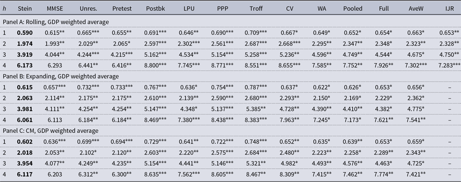
Note: This table presents the $1000 \times \text{MSFE}$
for different estimators.
$1000 \times \text{MSFE}$
for different estimators. $h$
in the first column shows the forecast horizon. Panels A–C report the results based on the GDP weighted average with rolling window of most recent 40 observations, the expanding window with the initial in-sample estimation period of 10 years, and the Clark and McCracken (Reference Clark and McCracken2010) method (CM), respectively. The GDP weighted average uses weights
$h$
in the first column shows the forecast horizon. Panels A–C report the results based on the GDP weighted average with rolling window of most recent 40 observations, the expanding window with the initial in-sample estimation period of 10 years, and the Clark and McCracken (Reference Clark and McCracken2010) method (CM), respectively. The GDP weighted average uses weights $w_i = Y_i/(\sum _{j=1}^{s} Y_j)$
, where
$w_i = Y_i/(\sum _{j=1}^{s} Y_j)$
, where $Y_i$
is the 2008 GDP in purchasing power terms for country
$Y_i$
is the 2008 GDP in purchasing power terms for country $i$
available from the GVAR database and
$i$
available from the GVAR database and $s = 7$
is the number of countries. In the heading of the table, Stein shows the MSFE for the proposed Stein-like shrinkage estimator, MMSE is for the proposed minimal mean squared error estimator, Unres. is for the unrestricted estimator, Pretest is for the pretest estimator, LPU is the one proposed by Lee et al. (Reference Lee, Parsaeian and Ullah2022a), PPP is the one proposed by Pesaran et al. (Reference Pesaran, Pick and Pranovich2013), Postbk, Troff, CV, WA, and Pooled are the five methods used in Pesaran and Timmermann (Reference Pesaran and Timmermann2007), Full uses the full sample of observations by ignoring the break, AveW is the method proposed by Pesaran and Pick (Reference Pesaran and Pick2011) with
$s = 7$
is the number of countries. In the heading of the table, Stein shows the MSFE for the proposed Stein-like shrinkage estimator, MMSE is for the proposed minimal mean squared error estimator, Unres. is for the unrestricted estimator, Pretest is for the pretest estimator, LPU is the one proposed by Lee et al. (Reference Lee, Parsaeian and Ullah2022a), PPP is the one proposed by Pesaran et al. (Reference Pesaran, Pick and Pranovich2013), Postbk, Troff, CV, WA, and Pooled are the five methods used in Pesaran and Timmermann (Reference Pesaran and Timmermann2007), Full uses the full sample of observations by ignoring the break, AveW is the method proposed by Pesaran and Pick (Reference Pesaran and Pick2011) with $w_{\text{min}}=0.1$
and 20 windows, and IJR is the optimal window method proposed by Inoue et al. (Reference Inoue, Jin and Rossi2017) with
$w_{\text{min}}=0.1$
and 20 windows, and IJR is the optimal window method proposed by Inoue et al. (Reference Inoue, Jin and Rossi2017) with $\underline{R}=\text{max}(1.5T^{2/3}, 20)$
and
$\underline{R}=\text{max}(1.5T^{2/3}, 20)$
and $\overline{R}=\text{min}(4T^{2/3}, T-h)$
. This table also shows the panel Diebold and Mariano (DM) test statistic for the Stein-like shrinkage forecast relative to each of the alternative methods as the benchmark. An asterisk represents statistically significance evidence in favor of the Stein-like shrinkage estimator according to the panel Diebold-Mariano test statistic. The
$\overline{R}=\text{min}(4T^{2/3}, T-h)$
. This table also shows the panel Diebold and Mariano (DM) test statistic for the Stein-like shrinkage forecast relative to each of the alternative methods as the benchmark. An asterisk represents statistically significance evidence in favor of the Stein-like shrinkage estimator according to the panel Diebold-Mariano test statistic. The $1\%$
,
$1\%$
, $5\%$
, and
$5\%$
, and $10\%$
significance levels are denoted by
$10\%$
significance levels are denoted by $^{***}$
,
$^{***}$
, $^{**}$
and
$^{**}$
and $^{*}$
, respectively.
$^{*}$
, respectively.
Table 2. Empirical results for forecasting output growth
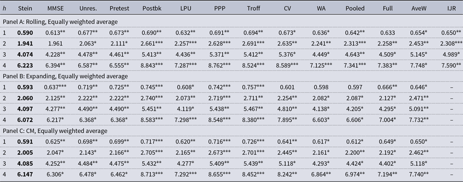
Note: See the notes to Table 1. The equal weights average uses $w_i = 1/s$
with
$w_i = 1/s$
with $s=7$
.
$s=7$
.
Based on the results in Tables 1–2, the forecasts based on the Stein-like shrinkage estimator and the minimal MSE estimator provide improved forecasts over the unrestricted estimator for different forecast horizons. With the GDP-PPP weighted average scheme, for the Stein-like shrinkage estimator (and the minimal MSE estimator), the improvement ranges from 2.7 to 11.3 (1.8 to 7.5) percent for the rolling window, from 2 to 16 (1.1 to 7.5) percent for the expanding window, and from 3.1 to 13.9 (1.7 to 7.6) percent for the CM method. With the equally weighted average scheme, these improvements range from 5.5 to 12.9 (2.9 to 9.5) percent for the rolling window, from 4.6 to 17.5 (2.4 to 8.6) percent for the expanding window, and from 5.1 to 15.3 (2.7 to 9.5) percent for the CM method. The results suggest that improvement using the equally weighted average scheme is slightly higher than those of the GDP-PPP weighted average scheme. Besides, the MSFE of the Stein-like shrinkage estimator is less than the minimal MSE estimator. All these results are consistent with our theoretical findings in Theorems 3–4, and Remark 3.
Furthermore, the MSFEs of the Stein-like shrinkage estimator outperform the other alternative estimators. To determine whether the Stein-like shrinkage estimator significantly outperforms the alternative methods, we report the panel version of the Diebold and Mariano (Reference Diebold and Mariano1995) test (DM) introduced by Pesaran et al. (Reference Pesaran, Schuermann and Smith2009) in Tables 1–2, in which we take each of the alternative methods as a benchmark (i.e., $DM_i$
is the benchmark method in which
$DM_i$
is the benchmark method in which $i$
represents the alternative methods such as MMSE, Unres., Pretest, Postbk, PPP, Troff, CV, WA, Pooled, Full, AveW, and IJR, respectively). In Tables 1–2, an asterisk represents statistically significance evidence in favor of the Stein-like shrinkage estimator according to the panel Diebold–Mariano test statistic. The
$i$
represents the alternative methods such as MMSE, Unres., Pretest, Postbk, PPP, Troff, CV, WA, Pooled, Full, AveW, and IJR, respectively). In Tables 1–2, an asterisk represents statistically significance evidence in favor of the Stein-like shrinkage estimator according to the panel Diebold–Mariano test statistic. The $1\%$
,
$1\%$
, $5\%$
, and
$5\%$
, and $10\%$
significance levels are denoted by
$10\%$
significance levels are denoted by $^{***}$
,
$^{***}$
, $^{**}$
, and
$^{**}$
, and $^{*}$
, respectively. The results show that the Stein-like shrinkage estimator significantly outperforms all benchmark models in the majority of cases at the
$^{*}$
, respectively. The results show that the Stein-like shrinkage estimator significantly outperforms all benchmark models in the majority of cases at the $1\%$
,
$1\%$
, $5\%$
, and
$5\%$
, and $10\%$
levels, for various forecast horizons,
$10\%$
levels, for various forecast horizons, $h = 1,2,3,4$
. Overall, the results show the advantages of using the SUR model in forecasting relative to a univariate time series model in terms of providing lower MSFE. As discussed in Bai et al. (Reference Bai, Lumsdaine and Stock1998) and Qu and Perron (Reference Qu and Perron2007), the break-point problem is one in which there are substantial payoffs for using multivariate rather than univariate techniques. The accuracy of break point estimation can be significantly improved by adding series that have common breaks, and the precision of the estimates increases with the number of equations in the system. The more accurate the break point is estimated, the better estimate of slope coefficients is obtained, which ultimately helps to have a better forecasts. Besides, the SUR model uses the cross-sectional information rather than ignoring them which helps to have a better estimate and hence forecast.
$h = 1,2,3,4$
. Overall, the results show the advantages of using the SUR model in forecasting relative to a univariate time series model in terms of providing lower MSFE. As discussed in Bai et al. (Reference Bai, Lumsdaine and Stock1998) and Qu and Perron (Reference Qu and Perron2007), the break-point problem is one in which there are substantial payoffs for using multivariate rather than univariate techniques. The accuracy of break point estimation can be significantly improved by adding series that have common breaks, and the precision of the estimates increases with the number of equations in the system. The more accurate the break point is estimated, the better estimate of slope coefficients is obtained, which ultimately helps to have a better forecasts. Besides, the SUR model uses the cross-sectional information rather than ignoring them which helps to have a better estimate and hence forecast.
6. Conclusion
In this paper, we introduce two estimators for estimating the slope coefficients of SUR models with cross-sectional dependence under structural breaks, which are then used for forecasting. The proposed Stein-like shrinkage estimator and the minimal MSE estimator are the weighted averages of the unrestricted estimator (i.e., using observations within each regime separately) and the restricted estimator. The averaging weight is proportional to the difference between the restricted and unrestricted estimators. Thus, for a large break size, a lower weight is assigned to the restricted estimator (which is biased) and more weight is assigned to the unrestricted estimator. The opposite is true for a small break size. We establish the asymptotic distribution and asymptotic risk for the proposed estimators and find the conditions under which they uniformly outperform the unrestricted estimator for any break size and break point. We also analytically and numerically compare the performance of the two proposed estimators. The results show that the Stein-like shrinkage estimator performs better than the minimal MSE estimator due to its smaller asymptotic risk. This out-performance is more clear under small break sizes. Monte Carlo simulations and the empirical application of forecasting output growth rates of G7 countries show the significant superiority of using the Stein-like shrinkage estimator over the alternative estimators.
Supplementary material
The supplementary material for this article can be found at http://doi.org/10.1017/S1365100523000329.
Acknowledgments
I would like to thank William A. Barnett (the editor), an associate editor, and anonymous referees for constructive comments on the paper.
A. Appendix: Mathematical details
LEMMA 1. Suppose $C$
and
$C$
and $D$
are two matrices, where
$D$
are two matrices, where $C_{n \times n}$
and
$C_{n \times n}$
and $D_{n \times m}$
, then
$D_{n \times m}$
, then
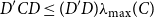 \begin{equation*} D'CD \leq (D'D) \lambda _{\text {max}}(C)\end{equation*}
in which $\lambda _{\text{max}}(C)$
is the maximum eigenvalue of
$\lambda _{\text{max}}(C)$
is the maximum eigenvalue of $C$
. See Bernstein (Reference Bernstein2005), p. 271 for the proof.
$C$
. See Bernstein (Reference Bernstein2005), p. 271 for the proof.
A.1. Proof of Theorem 1
Define $\widetilde{y}_t=\big (y_{1,t}, \dots, y_{N,t} \big )'$
,
$\widetilde{y}_t=\big (y_{1,t}, \dots, y_{N,t} \big )'$
, $\widetilde{x}_t=\text{diag}\big (x'_{\!\!1,t}, \dots, x'_{\!\!N,t}\big )$
, and
$\widetilde{x}_t=\text{diag}\big (x'_{\!\!1,t}, \dots, x'_{\!\!N,t}\big )$
, and $\widetilde{u}_t=\big (u_{1,t}, \dots, u_{N,t} \big )'$
. By stacking the model over individuals,
$\widetilde{u}_t=\big (u_{1,t}, \dots, u_{N,t} \big )'$
. By stacking the model over individuals, $i=1, \dots, N$
, for each time, we have
$i=1, \dots, N$
, for each time, we have
 \begin{equation} \widetilde{y}_t=\widetilde{x}_t \beta _{(t)}+\widetilde{u}_t, \quad \text{for} \quad t=1, \dots, T, \end{equation}
where
 \begin{equation} \beta _{(t)} \equiv \begin{cases} \beta _{(1)} & \mbox{for} \quad t=1, \dots, T_1, \\[5pt] \beta _{(2)} & \mbox{for} \quad t=T_1+1, \dots, T, \end{cases} \end{equation}
in which $\beta _{(1)}= \big (\beta' _{\!\!1(1)}, \dots, \beta' _{\!\!N(1)} \big )'$
and
$\beta _{(1)}= \big (\beta' _{\!\!1(1)}, \dots, \beta' _{\!\!N(1)} \big )'$
and $\beta _{(2)}= \big (\beta' _{\!\!1(2)}, \dots, \beta' _{\!\!N(2)} \big )'$
are
$\beta _{(2)}= \big (\beta' _{\!\!1(2)}, \dots, \beta' _{\!\!N(2)} \big )'$
are $Nk \times 1$
vectors of the slope coefficients. Define
$Nk \times 1$
vectors of the slope coefficients. Define $2Nk \times Nk$
selection matrices
$2Nk \times Nk$
selection matrices
 \begin{equation} G_1= \left[\begin{array}{c@{\quad}c@{\quad}c@{\quad}c@{\quad}c@{\quad}c} I_k & \mathbf{0} & \mathbf{0} & \mathbf{0} & \dots & \mathbf{0} \\[5pt] \mathbf{0} & \mathbf{0} & \mathbf{0} & \mathbf{0} & \dots & \mathbf{0} \\[5pt] \mathbf{0} &I_k & \mathbf{0} & \mathbf{0} & \dots & \mathbf{0} \\[5pt] & & & &\vdots &\\[5pt] \mathbf{0} & \mathbf{0} & \mathbf{0} & \mathbf{0} & \dots & \mathbf{0} \\[5pt] \end{array}\right], \end{equation}
and
 \begin{equation} G_2= \left[\begin{array}{c@{\quad}c@{\quad}c@{\quad}c@{\quad}c@{\quad}c} \mathbf{0} & \mathbf{0} & \mathbf{0} & \mathbf{0} & \dots & \mathbf{0} \\[5pt] I_k & \mathbf{0} & \mathbf{0} & \mathbf{0} & \dots & \mathbf{0} \\[5pt] \mathbf{0} & \mathbf{0} & \mathbf{0} & \mathbf{0} & \dots & \mathbf{0} \\[5pt] & & & &\vdots &\\[5pt] \mathbf{0} & \mathbf{0} & \mathbf{0} & \mathbf{0} & \dots & I_k \\[5pt] \end{array}\right], \end{equation}
such that $\boldsymbol{{b}}=G_1 \beta _{(1)}+G_2 \beta _{(2)}$
.
$\boldsymbol{{b}}=G_1 \beta _{(1)}+G_2 \beta _{(2)}$
.
Rewrite $\Omega$
in (6) as
$\Omega$
in (6) as $\Omega = \Sigma _{(1)} \otimes J_{(1)}+\Sigma _{(2)} \otimes J_{(2)}$
, where
$\Omega = \Sigma _{(1)} \otimes J_{(1)}+\Sigma _{(2)} \otimes J_{(2)}$
, where
 \begin{equation} \Sigma _{(1)}=\left[\begin{array}{c@{\quad}c@{\quad}c} \sigma _{11(1)} & \dots & \sigma _{1N(1)} \\[5pt] \vdots & \vdots & \vdots \\[5pt] \sigma _{N1(1)} & \dots & \sigma _{NN(1)} \end{array}\right], \end{equation}
 \begin{equation} \Sigma _{(2)}=\left[\begin{array}{c@{\quad}c@{\quad}c} \sigma _{11(2)} & \dots & \sigma _{1N(2)} \\[5pt] \vdots & \vdots & \vdots \\[5pt] \sigma _{N1(2)} & \dots & \sigma _{NN(2)} \end{array}\right], \end{equation}
are $N \times N$
matrices,
$N \times N$
matrices, $J_{(1)}= \begin{bmatrix} I_{T_1 } & \textbf{0}_{T_1 \times T-T_1} \\[5pt] \textbf{0}_{T-T_1 \times T_1} & \textbf{0}_{T-T_1 \times T-T_1} \end{bmatrix}$
, and
$J_{(1)}= \begin{bmatrix} I_{T_1 } & \textbf{0}_{T_1 \times T-T_1} \\[5pt] \textbf{0}_{T-T_1 \times T_1} & \textbf{0}_{T-T_1 \times T-T_1} \end{bmatrix}$
, and $J_{(2)}= \begin{bmatrix} \textbf{0}_{T_1 \times T_1 } & \textbf{0}_{T_1 \times T-T_1} \\[5pt] \textbf{0}_{T-T_1 \times T_1} & I_{T-T_1} \end{bmatrix}$
.
$J_{(2)}= \begin{bmatrix} \textbf{0}_{T_1 \times T_1 } & \textbf{0}_{T_1 \times T-T_1} \\[5pt] \textbf{0}_{T-T_1 \times T_1} & I_{T-T_1} \end{bmatrix}$
.
In the rest of the proof, we show the asymptotic normality of the feasible unrestricted estimator, $\widehat{\boldsymbol{{b}}}_{ur}= G_1 \widehat{\beta }_{(1)}^{\,fgls}+G_2 \widehat{\beta }_{(2)}^{\,fgls}$
. Initially, we derive the asymptotic distribution of the infeasible pre-break and post-break estimators, denoted by
$\widehat{\boldsymbol{{b}}}_{ur}= G_1 \widehat{\beta }_{(1)}^{\,fgls}+G_2 \widehat{\beta }_{(2)}^{\,fgls}$
. Initially, we derive the asymptotic distribution of the infeasible pre-break and post-break estimators, denoted by $\widehat{\beta }_{(1)}^{\,gls}$
and
$\widehat{\beta }_{(1)}^{\,gls}$
and $\widehat{\beta }_{(2)}^{\,gls}$
, respectively.
$\widehat{\beta }_{(2)}^{\,gls}$
, respectively.
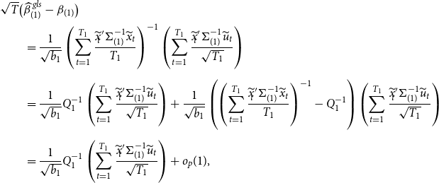 \begin{equation} \begin{aligned} & \sqrt{T}\big (\widehat{\beta }_{(1)}^{\,gls}-\beta _{(1)}\big ) \\ &\qquad = \frac{1}{\sqrt{b_1}} \left (\sum _{t=1}^{T_1} \frac{\widetilde{x}'_{\!\!t} \Sigma _{(1)}^{-1} \widetilde{x}_t}{T_1} \right)^{-1} \left (\sum _{t=1}^{T_1} \frac{\widetilde{x}'_{\!\!t} \Sigma _{(1)}^{-1} \widetilde{u}_t}{\sqrt{T_1}} \right)\\[5pt] &\qquad=\frac{1}{\sqrt{b_1}} Q_1^{-1} \left (\sum _{t=1}^{T_1} \frac{\widetilde{x}'_{\!\!t} \Sigma _{(1)}^{-1} \widetilde{u}_t}{\sqrt{T_1}} \right) +\frac{1}{\sqrt{b_1}} \left (\left (\sum _{t=1}^{T_1} \frac{\widetilde{x}'_{\!\!t} \Sigma _{(1)}^{-1} \widetilde{x}_t}{T_1} \right)^{-1}- Q_1^{-1} \right) \left (\sum _{t=1}^{T_1} \frac{\widetilde{x}'_{\!\!t} \Sigma _{(1)}^{-1} \widetilde{u}_t}{\sqrt{T_1}} \right)\\[5pt] &\qquad=\frac{1}{\sqrt{b_1}} Q_1^{-1} \left (\sum _{t=1}^{T_1} \frac{\widetilde{x}'_{\!\!t} \Sigma _{(1)}^{-1} \widetilde{u}_t}{\sqrt{T_1}} \right)+o_p(1), \end{aligned} \end{equation}
where the last equality holds because $\sum _{t=1}^{T_1} \frac{\widetilde{x}'_{\!\!t} \Sigma _{(1)}^{-1} \widetilde{x}_t}{T_1} \xrightarrow{p}{\mathbb{E}} \big (\widetilde{x}'_{\!\!t} \Sigma _{(1)}^{-1} \widetilde{x}_t \big ) \equiv Q_1$
which is implied by Assumptions 1 and 3. Also, we note that
$\sum _{t=1}^{T_1} \frac{\widetilde{x}'_{\!\!t} \Sigma _{(1)}^{-1} \widetilde{x}_t}{T_1} \xrightarrow{p}{\mathbb{E}} \big (\widetilde{x}'_{\!\!t} \Sigma _{(1)}^{-1} \widetilde{x}_t \big ) \equiv Q_1$
which is implied by Assumptions 1 and 3. Also, we note that
 \begin{equation} var \left (\sum _{t=1}^{T_1} \frac{\widetilde{x}'_{\!\!t} \Sigma _{(1)}^{-1} \widetilde{u}_t}{\sqrt{T_1}} \right)= \big (1/T_1 \big ){\mathbb{E}} \left (\sum _{t=1}^{T_1} \widetilde{x}'_{\!\!t} \Sigma _{(1)}^{-1} \widetilde{x}_t \right)= Q_1= O(1) \lt \infty, \end{equation}
which implies that $\sum _{t=1}^{T_1} \frac{\widetilde{x}'_{\!\!t} \Sigma _{(1)}^{-1} \widetilde{u}_t}{\sqrt{T_1}}=O_p(1)$
. Therefore, by central limit theorem,
$\sum _{t=1}^{T_1} \frac{\widetilde{x}'_{\!\!t} \Sigma _{(1)}^{-1} \widetilde{u}_t}{\sqrt{T_1}}=O_p(1)$
. Therefore, by central limit theorem,
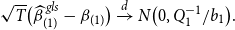 \begin{equation} \begin{aligned} \sqrt{T}\big (\widehat{\beta }_{(1)}^{\,gls}-\beta _{(1)}\big ) \xrightarrow{d} N \big (0, Q_1^{-1}/ b_1 \big ). \end{aligned} \end{equation}
Similarly, the asymptotic distribution of the infeasible post-break estimator is
 \begin{equation} \begin{aligned} \sqrt{T}\big (\widehat{\beta }_{(2)}^{\,gls}-\beta _{(2)}\big ) &= \frac{1}{\sqrt{1-b_1}} \left (\sum _{t=T_1+1}^{T} \frac{\widetilde{x}'_{\!\!t} \Sigma _{(2)}^{-1} \widetilde{x}_t}{T-T_1} \right)^{-1} \left (\sum _{t=T_1+1}^{T} \frac{\widetilde{x}'_{\!\!t} \Sigma _{(2)}^{-1} \widetilde{u}_t}{\sqrt{T-T_1}} \right)\\[5pt] &\xrightarrow{d} N \big (0, Q_2^{-1}/ (1-b_1) \big ), \end{aligned} \end{equation}
where $\sum _{t=T_1+1}^{T} \frac{\widetilde{x}'_{\!\!t} \Sigma _{(2)}^{-1} \widetilde{x}_t}{T-T_1} \xrightarrow{p}{\mathbb{E}} \big (\widetilde{x}'_{\!\!t} \Sigma _{(2)}^{-1} \widetilde{x}_t \big ) \equiv Q_2$
.
$\sum _{t=T_1+1}^{T} \frac{\widetilde{x}'_{\!\!t} \Sigma _{(2)}^{-1} \widetilde{x}_t}{T-T_1} \xrightarrow{p}{\mathbb{E}} \big (\widetilde{x}'_{\!\!t} \Sigma _{(2)}^{-1} \widetilde{x}_t \big ) \equiv Q_2$
.
Now, we provide the asymptotic distribution of the feasible pre-break estimator, $\widehat{\beta }_{(1)}^{\,fgls}$
.
$\widehat{\beta }_{(1)}^{\,fgls}$
.
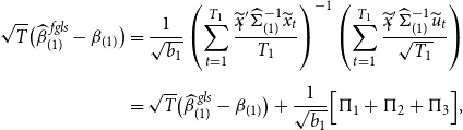 \begin{equation} \begin{aligned} \sqrt{T}\big (\widehat{\beta }_{(1)}^{\,fgls}-\beta _{(1)}\big )&= \frac{1}{\sqrt{b_1}} \left (\sum _{t=1}^{T_1} \frac{\widetilde{x}'_{\!\!t} \widehat{\Sigma }_{(1)}^{-1} \widetilde{x}_t}{T_1} \right)^{-1} \left (\sum _{t=1}^{T_1} \frac{\widetilde{x}'_{\!\!t} \widehat{\Sigma }_{(1)}^{-1} \widetilde{u}_t}{\sqrt{T_1}} \right)\\[5pt] &= \sqrt{T}\big (\widehat{\beta }_{(1)}^{\,gls}-\beta _{(1)}\big )+ \frac{1}{\sqrt{b_1}} \Big [\Pi _1+\Pi _2+\Pi _3\Big ], \end{aligned} \end{equation}
where
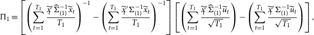 \begin{equation} \begin{aligned} \Pi _1 &\equiv \left[ \left (\sum _{t=1}^{T_1} \frac{\widetilde{x}'_{\!\!t} \widehat{\Sigma }_{(1)}^{-1} \widetilde{x}_t}{T_1} \right)^{-1}-\left (\sum _{t=1}^{T_1} \frac{\widetilde{x}'_{\!\!t}{\Sigma }_{(1)}^{-1} \widetilde{x}_t}{T_1} \right)^{-1} \right] \left[\left (\sum _{t=1}^{T_1} \frac{\widetilde{x}'_{\!\!t} \widehat{\Sigma }_{(1)}^{-1} \widetilde{u}_t}{\sqrt{T_1}} \right)-\left (\sum _{t=1}^{T_1} \frac{\widetilde{x}'_{\!\!t}{\Sigma }_{(1)}^{-1} \widetilde{u}_t}{\sqrt{T_1}} \right) \right], \end{aligned} \end{equation}
 \begin{equation} \begin{aligned} \Pi _2 & \equiv \left (\sum _{t=1}^{T_1} \frac{\widetilde{x}'_{\!\!t}{\Sigma }_{(1)}^{-1} \widetilde{x}_t}{T_1} \right)^{-1} \left[\left (\sum _{t=1}^{T_1} \frac{\widetilde{x}'_{\!\!t} \widehat{\Sigma }_{(1)}^{-1} \widetilde{u}_t}{\sqrt{T_1}} \right)-\left (\sum _{t=1}^{T_1} \frac{\widetilde{x}'_{\!\!t}{\Sigma }_{(1)}^{-1} \widetilde{u}_t}{\sqrt{T_1}} \right) \right], \end{aligned} \end{equation}
and
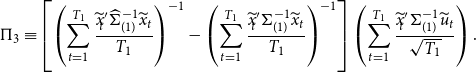 \begin{equation} \begin{aligned} \Pi _3 &\equiv \left[\left (\sum _{t=1}^{T_1} \frac{\widetilde{x}'_{\!\!t} \widehat{\Sigma }_{(1)}^{-1} \widetilde{x}_t}{T_1} \right)^{-1}-\left (\sum _{t=1}^{T_1} \frac{\widetilde{x}'_{\!\!t}{\Sigma }_{(1)}^{-1} \widetilde{x}_t}{T_1} \right)^{-1} \right]\left (\sum _{t=1}^{T_1} \frac{\widetilde{x}'_{\!\!t}{\Sigma }_{(1)}^{-1} \widetilde{u}_t}{\sqrt{T_1}} \right). \end{aligned} \end{equation}
We note that
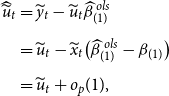 \begin{equation} \begin{aligned} \widehat{\widetilde{u}}_t &=\widetilde{y}_t-\widetilde{u}_t \widehat{\beta }_{(1)}^{\,ols}\\[5pt] &= \widetilde{u}_t-\widetilde{x}_t \big (\widehat{\beta }_{(1)}^{\,ols}-\beta _{(1)} \big )\\[5pt] &=\widetilde{u}_t+o_p(1), \end{aligned} \end{equation}
where $\widehat{\beta }_{(1)}^{\,ols}= \left (\widehat{\beta }_{1(1)}^{\,ols^{\prime}}, \dots, \widehat{\beta }_{N(1)}^{\,ols^{\prime}} \right)'$
. Therefore,
$\widehat{\beta }_{(1)}^{\,ols}= \left (\widehat{\beta }_{1(1)}^{\,ols^{\prime}}, \dots, \widehat{\beta }_{N(1)}^{\,ols^{\prime}} \right)'$
. Therefore, $\widehat{\Sigma }_{(1)}= \frac{1}{T_1} \sum _{1}^{T_1} \widehat{\widetilde{u}}_t \widehat{\widetilde{u}}_t'= \Sigma _{(1)}+o_p(1)$
. It follows that
$\widehat{\Sigma }_{(1)}= \frac{1}{T_1} \sum _{1}^{T_1} \widehat{\widetilde{u}}_t \widehat{\widetilde{u}}_t'= \Sigma _{(1)}+o_p(1)$
. It follows that $\left (\sum _{t=1}^{T_1} \frac{\widetilde{x}'_{\!\!t} \widehat{\Sigma }_{(1)}^{-1} \widetilde{x}_t}{T_1} \right)-\left (\sum _{t=1}^{T_1} \frac{\widetilde{x}'_{\!\!t}{\Sigma }_{(1)}^{-1} \widetilde{x}_t}{T_1} \right)=o_p(1)$
,
$\left (\sum _{t=1}^{T_1} \frac{\widetilde{x}'_{\!\!t} \widehat{\Sigma }_{(1)}^{-1} \widetilde{x}_t}{T_1} \right)-\left (\sum _{t=1}^{T_1} \frac{\widetilde{x}'_{\!\!t}{\Sigma }_{(1)}^{-1} \widetilde{x}_t}{T_1} \right)=o_p(1)$
, $\left (\sum _{t=1}^{T_1} \frac{\widetilde{x}'_{\!\!t} \widehat{\Sigma }_{(1)}^{-1} \widetilde{x}_t}{T_1} \right)^{-1}-\left (\sum _{t=1}^{T_1} \frac{\widetilde{x}'_{\!\!t}{\Sigma }_{(1)}^{-1} \widetilde{x}_t}{T_1} \right)^{-1}=o_p(1)$
, and
$\left (\sum _{t=1}^{T_1} \frac{\widetilde{x}'_{\!\!t} \widehat{\Sigma }_{(1)}^{-1} \widetilde{x}_t}{T_1} \right)^{-1}-\left (\sum _{t=1}^{T_1} \frac{\widetilde{x}'_{\!\!t}{\Sigma }_{(1)}^{-1} \widetilde{x}_t}{T_1} \right)^{-1}=o_p(1)$
, and $\left (\sum _{t=1}^{T_1} \frac{\widetilde{x}'_{\!\!t} \widehat{\Sigma }_{(1)}^{-1} \widetilde{u}_t}{\sqrt{T_1}} \right)-\left (\sum _{t=1}^{T_1} \frac{\widetilde{x}'_{\!\!t}{\Sigma }_{(1)}^{-1} \widetilde{u}_t}{\sqrt{T_1}} \right)=o_p(1)$
. Thus,
$\left (\sum _{t=1}^{T_1} \frac{\widetilde{x}'_{\!\!t} \widehat{\Sigma }_{(1)}^{-1} \widetilde{u}_t}{\sqrt{T_1}} \right)-\left (\sum _{t=1}^{T_1} \frac{\widetilde{x}'_{\!\!t}{\Sigma }_{(1)}^{-1} \widetilde{u}_t}{\sqrt{T_1}} \right)=o_p(1)$
. Thus, $\Pi _1=o_p(1), \Pi _2=o_p(1)$
and
$\Pi _1=o_p(1), \Pi _2=o_p(1)$
and $\Pi _3=o_p(1)$
. As a result, using central limit theorem, the asymptotic distribution of the feasible pre-break estimator in (A11) is
$\Pi _3=o_p(1)$
. As a result, using central limit theorem, the asymptotic distribution of the feasible pre-break estimator in (A11) is
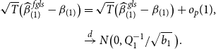 \begin{equation} \begin{aligned} \sqrt{T}\big (\widehat{\beta }_{(1)}^{\,fgls}-\beta _{(1)}\big ) &= \sqrt{T}\big (\widehat{\beta }_{(1)}^{\,gls}-\beta _{(1)}\big ) +o_p(1),\\[5pt] &\xrightarrow{d} N \big (0, Q_1^{-1}/ \sqrt{b_1} \ \big ). \end{aligned} \end{equation}
Similarly, the asymptotic distribution of the feasible post-break estimator is
 \begin{equation} \begin{aligned} \sqrt{T}\big (\widehat{\beta }_{(2)}^{\,fgls}-\beta _{(2)}\big ) \xrightarrow{d} N \big (0, Q_2^{-1}/ (1-b_1) \ \big ). \end{aligned} \end{equation}
Therefore, it immediately follows that
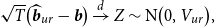 \begin{equation} \begin{aligned} \sqrt{T} \big ( \widehat{\boldsymbol{{b}}}_{ur}-\boldsymbol{{b}} \big ) \xrightarrow{d} Z \sim \text{N} \big (0, V_{ur} \big ), \end{aligned} \end{equation}
where $V_{ur}= \left ({\mathbb{E}} \big ( \frac{X'{\Omega }^{-1} X}{T}\big )\right)^{-1}.$
Furthermore, the asymptotic distribution of the restricted estimator is
 \begin{equation} \begin{aligned} \sqrt{T} \big (\widehat{\boldsymbol{{b}}}_r- \boldsymbol{{b}}\big ) &=\sqrt{T} \big ( \widehat{\boldsymbol{{b}}}_{ur} - \boldsymbol{{b}} \big )- \big ( X' \widehat{\Omega }^{-1} X \big )^{-1} R' \ \Big [R\big ( X' \widehat{\Omega }^{-1} X\big )^{-1} R' \Big ]^{-1} \sqrt{T} \big ( R\widehat{\boldsymbol{{b}}}_{ur}-\boldsymbol{{r}}-R\boldsymbol{{b}} + R\boldsymbol{{b}} \big )\\[5pt] & \xrightarrow{d} Z-V_{ur} R' \Big [R V_{ur} R' \Big ]^{-1} R (Z+\boldsymbol{{h}}), \end{aligned} \end{equation}
where $R\boldsymbol{{b}}=\boldsymbol{{r}}+R\boldsymbol{{h}}/\sqrt{T}$
. Thus, the difference between the restricted and unrestricted estimators is
$R\boldsymbol{{b}}=\boldsymbol{{r}}+R\boldsymbol{{h}}/\sqrt{T}$
. Thus, the difference between the restricted and unrestricted estimators is
 \begin{equation} \begin{aligned} \sqrt{T} \big (\widehat{\boldsymbol{{b}}}_{ur}- \widehat{\boldsymbol{{b}}}_r \big ) & \xrightarrow{d} V_{ur} R' \Big [R V_{ur} R' \Big ]^{-1} R (Z+\boldsymbol{{h}}). \end{aligned} \end{equation}
Using (A20), distribution of $D_T$
in (17) is straightforward. Also, using (A18) and (A20), the asymptotic distribution of the Stein-like shrinkage estimator is
$D_T$
in (17) is straightforward. Also, using (A18) and (A20), the asymptotic distribution of the Stein-like shrinkage estimator is
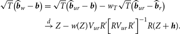 \begin{equation} \begin{aligned} \sqrt{T} \big (\widehat{\boldsymbol{{b}}}_w-\boldsymbol{{b}} \big ) &= \sqrt{T}\big (\widehat{\boldsymbol{{b}}}_{ur}-\boldsymbol{{b}} \big )- w_T \sqrt{T} \big (\widehat{\boldsymbol{{b}}}_{ur}-\widehat{\boldsymbol{{b}}}_{r} \big )\\[3pt] & \xrightarrow{d} Z-w(Z) V_{ur} R' \Big [R V_{ur} R' \Big ]^{-1} R (Z+\boldsymbol{{h}}). \end{aligned} \end{equation}
This completes the proof of Theorem 1.
A.2. Proof of Theorem 2
By having the results of Theorem 1, we follow along the lines of Hansen (Reference Hansen2016) to prove Theorem 2. We derive the asymptotic risk of the Stein-like shrinkage estimator for any positive definite weight matrix $\mathbb{W}$
. Ultimately, we set
$\mathbb{W}$
. Ultimately, we set ${\mathbb{W}}=V_{ur}^{-1}$
which gives the results presented in Theorem 2. The asymptotic risk of the Stein-like shrinkage estimator can be calculated as
${\mathbb{W}}=V_{ur}^{-1}$
which gives the results presented in Theorem 2. The asymptotic risk of the Stein-like shrinkage estimator can be calculated as
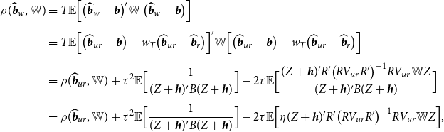 \begin{equation} \begin{aligned} \rho (\widehat{\boldsymbol{{b}}}_w,{\mathbb{W}}) &=T{\mathbb{E}} \Big [ \big (\widehat{\boldsymbol{{b}}}_w-\boldsymbol{{b}} \big )'{\mathbb{W}} \ \big (\widehat{\boldsymbol{{b}}}_w-\boldsymbol{{b}} \big ) \Big ]\\[4pt] &= T{\mathbb{E}} \Big [ \big (\widehat{\boldsymbol{{b}}}_{ur}-\boldsymbol{{b}}\big )-w_T \big (\widehat{\boldsymbol{{b}}}_{ur}-\widehat{\boldsymbol{{b}}}_{r} \big ) \Big ]'{\mathbb{W}} \Big [ \big (\widehat{\boldsymbol{{b}}}_{ur}-\boldsymbol{{b}} \big )-w_T \big (\widehat{\boldsymbol{{b}}}_{ur}-\widehat{\boldsymbol{{b}}}_{r} \big )\Big ]\\[4pt] &= \rho (\widehat{\boldsymbol{{b}}}_{ur},{\mathbb{W}})+ \tau ^2{\mathbb{E}} \Big [ \frac{1}{(Z+\boldsymbol{{h}})' B (Z+\boldsymbol{{h}})}\Big ] -2 \tau{\mathbb{E}} \Big [ \frac{(Z+\boldsymbol{{h}})' R' \big (R V_{ur} R' \big )^{-1} R V_{ur}{\mathbb{W}} Z}{(Z+\boldsymbol{{h}})' B (Z+\boldsymbol{{h}})}\Big ]\\[4pt] &= \rho (\widehat{\boldsymbol{{b}}}_{ur},{\mathbb{W}})+ \tau ^2{\mathbb{E}} \Big [ \frac{1}{(Z+\boldsymbol{{h}})' B (Z+\boldsymbol{{h}})}\Big ] -2 \tau{\mathbb{E}} \Big [\eta (Z+\boldsymbol{{h}})' R' \big (R V_{ur} R' \big )^{-1} R V_{ur}{\mathbb{W}} Z \Big ],\\[4pt] \end{aligned} \end{equation}
where $\eta (x)= \big (\frac{1}{x'Bx} \big )x$
. Using the Stein’s lemma (see lemma 2 in the appendix of Hansen (Reference Hansen2016)), we simplify the last term in (A22) as
$\eta (x)= \big (\frac{1}{x'Bx} \big )x$
. Using the Stein’s lemma (see lemma 2 in the appendix of Hansen (Reference Hansen2016)), we simplify the last term in (A22) as
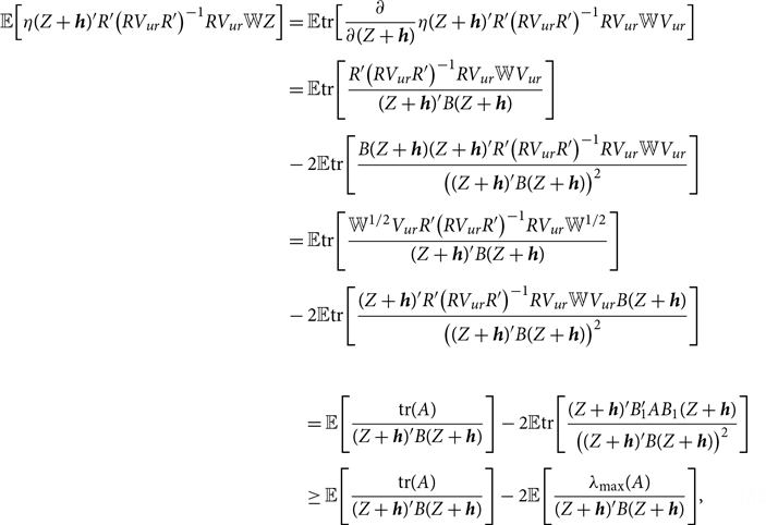 \begin{align}{\mathbb{E}} \Big [\eta (Z+\boldsymbol{{h}})' R' \big (R V_{ur} R' \big )^{-1} R V_{ur}{\mathbb{W}} Z \Big ] &={\mathbb{E}} \text{tr} \Big [ \frac{\partial }{\partial (Z+\boldsymbol{{h}})}\eta (Z+\boldsymbol{{h}})' R' \big (R V_{ur} R' \big )^{-1} R V_{ur}{\mathbb{W}} V_{ur} \Big ]\nonumber \\[4pt] &={\mathbb{E}} \text{tr} \Bigg [ \frac{R' \big (R V_{ur} R' \big )^{-1} R V_{ur}{\mathbb{W}} V_{ur}}{(Z+\boldsymbol{{h}})' B (Z+\boldsymbol{{h}})}\Bigg ] \nonumber \\[4pt] &-2{\mathbb{E}} \text{tr} \Bigg [ \frac{B (Z+\boldsymbol{{h}})(Z+\boldsymbol{{h}})'R' \big (R V_{ur} R' \big )^{-1} R V_{ur}{\mathbb{W}} V_{ur}}{\left ((Z+\boldsymbol{{h}})' B (Z+\boldsymbol{{h}})\right)^2}\Bigg ]\nonumber \\[4pt] &={\mathbb{E}} \text{tr} \Bigg [ \frac{{\mathbb{W}}^{1/2} V_{ur} R' \big (R V_{ur} R' \big )^{-1} R V_{ur}{\mathbb{W}}^{1/2}}{(Z+\boldsymbol{{h}})' B (Z+\boldsymbol{{h}})}\Bigg ] \nonumber \\[4pt] &-2{\mathbb{E}} \text{tr} \Bigg [ \frac{(Z+\boldsymbol{{h}})'R' \big (R V_{ur} R' \big )^{-1} R V_{ur}{\mathbb{W}} V_{ur} B(Z+\boldsymbol{{h}})}{\left ((Z+\boldsymbol{{h}})' B (Z+\boldsymbol{{h}})\right)^2}\Bigg ]\nonumber \\ &={\mathbb{E}} \Bigg [ \frac{\text{tr}(A) }{(Z+\boldsymbol{{h}})' B (Z+\boldsymbol{{h}})}\Bigg ]-2{\mathbb{E}} \text{tr} \Bigg [ \frac{(Z+\boldsymbol{{h}})' B'_{\!\!1}A B_1 (Z+\boldsymbol{{h}})}{\left ((Z+\boldsymbol{{h}})' B (Z+\boldsymbol{{h}})\right)^2}\Bigg ]\nonumber \\[4pt] & \geq{\mathbb{E}} \Bigg [ \frac{\text{tr}(A) }{(Z+\boldsymbol{{h}})' B (Z+\boldsymbol{{h}})}\Bigg ]-2{\mathbb{E}} \Bigg [ \frac{ \lambda _{\text{max}}(A)}{(Z+\boldsymbol{{h}})' B (Z+\boldsymbol{{h}})}\Bigg ], \end{align}
where $A \equiv{\mathbb{W}}^{1/2} V_{ur} R' \Big [R V_{ur} R' \Big ]^{-1} R V_{ur}{\mathbb{W}}^{1/2}$
,
$A \equiv{\mathbb{W}}^{1/2} V_{ur} R' \Big [R V_{ur} R' \Big ]^{-1} R V_{ur}{\mathbb{W}}^{1/2}$
, $B \equiv R' \Big [R V_{ur} R' \Big ]^{-1} R V_{ur}{\mathbb{W}} V_{ur} R' \ \Big [R \ V_{ur} R' \Big ]^{-1} R$
,
$B \equiv R' \Big [R V_{ur} R' \Big ]^{-1} R V_{ur}{\mathbb{W}} V_{ur} R' \ \Big [R \ V_{ur} R' \Big ]^{-1} R$
, $B_1 \equiv{\mathbb{W}}^{1/2} V_{ur} R' \big (R V_{ur} R' \big )^{-1} R$
,
$B_1 \equiv{\mathbb{W}}^{1/2} V_{ur} R' \big (R V_{ur} R' \big )^{-1} R$
, $R' \big (R V_{ur} R' \big )^{-1} R V_{ur}{\mathbb{W}} V_{ur} B=B'_{\!\!1}A B_1$
, and
$R' \big (R V_{ur} R' \big )^{-1} R V_{ur}{\mathbb{W}} V_{ur} B=B'_{\!\!1}A B_1$
, and $B'_{\!\!1}B_1=B$
. Note that
$B'_{\!\!1}B_1=B$
. Note that $\frac{\partial }{\partial x}\eta (x)'= \left(\frac{1}{x'Bx}\right) I - \frac{2}{(x'Bx)^2} Bxx'.$
Also, we use Lemma 1 to get the last inequality. Plugging (A23) into (A22) produces
$\frac{\partial }{\partial x}\eta (x)'= \left(\frac{1}{x'Bx}\right) I - \frac{2}{(x'Bx)^2} Bxx'.$
Also, we use Lemma 1 to get the last inequality. Plugging (A23) into (A22) produces
 \begin{equation} \begin{aligned} \rho (\widehat{\boldsymbol{{b}}}_w,{\mathbb{W}}) & \lt \rho (\widehat{\boldsymbol{{b}}}_{ur},{\mathbb{W}})+ \tau ^2{\mathbb{E}} \Big [ \frac{1}{(Z+\boldsymbol{{h}})' B (Z+\boldsymbol{{h}})}\Big ] -2 \tau \Big [ \frac{\text{tr}(A)-2 \lambda _{\text{max}}(A)}{(Z+\boldsymbol{{h}})' B (Z+\boldsymbol{{h}})}\Big ]\\[5pt] &= \rho (\widehat{\boldsymbol{{b}}}_{ur},{\mathbb{W}})- \tau{\mathbb{E}} \Big [ \frac{2 \big (\text{tr}(A)- 2\lambda _{\text{max}}(A)\big ) -\tau }{(Z+\boldsymbol{{h}})' B (Z+\boldsymbol{{h}})}\Big ]\\[5pt] & \lt \rho (\widehat{\boldsymbol{{b}}}_{ur},{\mathbb{W}})- \tau \Big [ \frac{2 \big (\text{tr}(A)-2 \lambda _{\text{max}}(A)\big ) -\tau }{{\mathbb{E}}(Z+\boldsymbol{{h}})' B (Z+\boldsymbol{{h}})}\Big ]\\[5pt] &= \rho (\widehat{\boldsymbol{{b}}}_{ur},{\mathbb{W}})- \tau \Big [ \frac{2 \big (\text{tr}(A)- 2\lambda _{\text{max}}(A)\big ) -\tau }{ (c+1) \text{tr} (A)}\Big ], \end{aligned} \end{equation}
where the last inequality is based on the Jensen’s inequality. Notice that
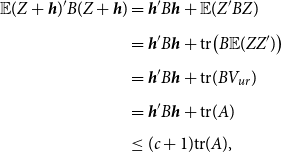 \begin{align}{\mathbb{E}}(Z+\boldsymbol{{h}})' B (Z+\boldsymbol{{h}}) &= \boldsymbol{{h}}'B\boldsymbol{{h}}+{\mathbb{E}} (Z'BZ) \nonumber \\[5pt] &=\boldsymbol{{h}}'B\boldsymbol{{h}}+ \text{tr} \big (B{\mathbb{E}} (ZZ')\big )\nonumber \\[5pt] &=\boldsymbol{{h}}'B\boldsymbol{{h}}+ \text{tr} (BV_{ur})\nonumber \\[5pt] &=\boldsymbol{{h}}'B\boldsymbol{{h}}+ \text{tr} (A)\nonumber \\[5pt] & \leq (c+1) \text{tr} (A), \end{align}
in which for any $0 \lt c \lt \infty$
, we define a ball such that
$0 \lt c \lt \infty$
, we define a ball such that $H(c)= \{ \boldsymbol{{h}}\;:\; \boldsymbol{{h}}'B\boldsymbol{{h}} \leq \text{tr} (A) \ c \}$
. When
$H(c)= \{ \boldsymbol{{h}}\;:\; \boldsymbol{{h}}'B\boldsymbol{{h}} \leq \text{tr} (A) \ c \}$
. When ${\mathbb{W}}=V_{ur}^{-1}$
,
${\mathbb{W}}=V_{ur}^{-1}$
, $\text{tr}(A)=Nk$
. This completes the proof of Theorem 2.
$\text{tr}(A)=Nk$
. This completes the proof of Theorem 2.
A.3. Proof of equation (26)
Here, we obtain the optimal weight, $\widehat{\gamma }^*_{opt}$
, for the minimal mean squared error estimator for any positive definite weight matrix
$\widehat{\gamma }^*_{opt}$
, for the minimal mean squared error estimator for any positive definite weight matrix $\mathbb{W}$
. Using the asymptotic distribution of the estimators in (15) and (16), the asymptotic risk for the minimal mean squared error estimator is
$\mathbb{W}$
. Using the asymptotic distribution of the estimators in (15) and (16), the asymptotic risk for the minimal mean squared error estimator is
 \begin{equation} \begin{aligned} \rho (\widehat{\boldsymbol{{b}}}_\gamma,{\mathbb{W}})&=\rho (\widehat{\boldsymbol{{b}}}_{ur},{\mathbb{W}})+ \gamma ^2{\mathbb{E}} \big [(Z+\boldsymbol{{h}})'R' \big (R V_{ur} R' \big )^{-1} R V_{ur}{\mathbb{W}} V_{ur} R' \big (R V_{ur} R' \big )^{-1} R (Z+\boldsymbol{{h}}) \big ]\\[5pt] &- 2 \gamma{\mathbb{E}} \big [(Z+\boldsymbol{{h}})'R' \big (R V_{ur} R' \big )^{-1} R V_{ur}{\mathbb{W}} Z \big ]\\[5pt] &= \rho (\widehat{\boldsymbol{{b}}}_{ur},{\mathbb{W}})+ \gamma ^2 \boldsymbol{{h}}'B\boldsymbol{{h}}+\gamma ^2 \ \text{tr}{\mathbb{E}} \big (ZZ' B\big )-2 \gamma \ \text{tr}{\mathbb{E}} \big ( ZZ'R' \big (R V_{ur} R' \big )^{-1} R V_{ur}{\mathbb{W}} \big )\\[5pt] &= \rho (\widehat{\boldsymbol{{b}}}_{ur},{\mathbb{W}})+ \gamma ^2 \big (\boldsymbol{{h}}' B \boldsymbol{{h}}+ \text{tr}(A) \big ) -2 \gamma \ \text{tr}(A), \end{aligned} \end{equation}
where $\text{tr}(V_{ur}B)=\text{tr}(A)$
. By minimizing the asymptotic risk with respect to
$\text{tr}(V_{ur}B)=\text{tr}(A)$
. By minimizing the asymptotic risk with respect to $\gamma$
in (A26), the optimal value of the weight denoted by
$\gamma$
in (A26), the optimal value of the weight denoted by $\gamma ^*_{opt}$
is
$\gamma ^*_{opt}$
is
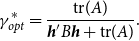 \begin{equation} \gamma ^*_{opt}=\frac{\text{tr}(A)}{\boldsymbol{{h}}' B \boldsymbol{{h}}+\text{tr}(A)}. \end{equation}
To find an unbiased estimator for the denominator of the weight in (A27), we note that
 \begin{equation} \begin{aligned}{\mathbb{E}}(\widehat{\boldsymbol{{h}}}' B \widehat{\boldsymbol{{h}}}) &= T{\mathbb{E}} \big [(\widehat{\boldsymbol{{b}}}_{ur}- \widehat{\boldsymbol{{b}}}_r)' B (\widehat{\boldsymbol{{b}}}_{ur}- \widehat{\boldsymbol{{b}}}_r) \big ]\\[5pt] &= \boldsymbol{{h}}' B \boldsymbol{{h}}+\text{tr}(A), \end{aligned} \end{equation}
where the unbiased estimator for $\boldsymbol{{h}}' B \boldsymbol{{h}}$
is
$\boldsymbol{{h}}' B \boldsymbol{{h}}$
is ${\mathbb{E}}(\widehat{\boldsymbol{{h}}}' B \widehat{\boldsymbol{{h}}})-\text{tr}(A)$
. By plugging this into the denominator of (A27), we have
${\mathbb{E}}(\widehat{\boldsymbol{{h}}}' B \widehat{\boldsymbol{{h}}})-\text{tr}(A)$
. By plugging this into the denominator of (A27), we have
 \begin{equation} \begin{aligned} \widehat{\gamma }^*_{opt}=\frac{\text{tr}(A)}{\widehat{\boldsymbol{{h}}}' B \widehat{\boldsymbol{{h}}}} & =\frac{\text{tr}(A)}{T(\widehat{\boldsymbol{{b}}}_{ur}- \widehat{\boldsymbol{{b}}}_r)'{\mathbb{W}} (\widehat{\boldsymbol{{b}}}_{ur}- \widehat{\boldsymbol{{b}}}_r)}= \frac{\text{tr}(A)}{D_T}, \end{aligned} \end{equation}
where the second equality holds noting that $V_{ur} R' \Big [R V_{ur} R' \Big ]^{-1} R (\widehat{\boldsymbol{{b}}}_{ur}- \widehat{\boldsymbol{{b}}}_r)=\widehat{\boldsymbol{{b}}}_{ur}- \widehat{\boldsymbol{{b}}}_r$
.
$V_{ur} R' \Big [R V_{ur} R' \Big ]^{-1} R (\widehat{\boldsymbol{{b}}}_{ur}- \widehat{\boldsymbol{{b}}}_r)=\widehat{\boldsymbol{{b}}}_{ur}- \widehat{\boldsymbol{{b}}}_r$
.
A.4. Proof of Theorem 4
The asymptotic risk of the minimal mean squared error estimator after plugging the optimal value of the weight in (A29) is
 \begin{align} \rho (\widehat{\boldsymbol{{b}}}_\gamma,{\mathbb{W}}) &= \rho (\widehat{\boldsymbol{{b}}}_{ur},{\mathbb{W}})+ \big ( \text{tr}(A) \big )^2{\mathbb{E}} \Big [ \frac{1}{(Z+\boldsymbol{{h}})' B (Z+\boldsymbol{{h}})}\Big ]\nonumber \\[5pt] & -2 \ \text{tr}(A){\mathbb{E}} \Big [\eta (Z+\boldsymbol{{h}})' R' \big (R V_{ur} R' \big )^{-1} R \big ( X'{\Omega }^{-1} X \big )^{-1}{\mathbb{W}} Z \Big ]\nonumber \\[5pt] &\leq \rho (\widehat{\boldsymbol{{b}}}_{ur},{\mathbb{W}})+ \big ( \text{tr}(A) \big )^2{\mathbb{E}} \Big [ \frac{1}{(Z+\boldsymbol{{h}})' B (Z+\boldsymbol{{h}})}\Big ] \nonumber \\[5pt] &-2 \ \text{tr}(A) \big [\text{tr}(A)-2 \lambda _{\text{max}}(A) \big ]{\mathbb{E}} \Big [ \frac{1}{(Z+\boldsymbol{{h}})' B (Z+\boldsymbol{{h}})}\Big ]\nonumber \\[5pt] &\leq \rho (\widehat{\boldsymbol{{b}}}_{ur},{\mathbb{W}})- \frac{\text{tr}(A)- 4\lambda _{\text{max}}(A)}{(c+1)}, \end{align}
where in the last two inequalities we use (A23) and the Jensen’s inequality, respectively. Plugging ${\mathbb{W}}=V_{ur}^{-1}$
completes the proof of Theorem 4.
${\mathbb{W}}=V_{ur}^{-1}$
completes the proof of Theorem 4.
Furthermore, the difference between the asymptotic risk of the Stein-like shrinkage estimator and that of the minimal mean squared error estimator for any positive definite matrix $\mathbb{W}$
is
$\mathbb{W}$
is
 \begin{equation} \rho (\widehat{\boldsymbol{{b}}}_w,{\mathbb{W}})- \rho (\widehat{\boldsymbol{{b}}}_\gamma,{\mathbb{W}})= \frac{-4 \ \lambda _{\text{max}}(A)}{(c+1) \ d}\lt 0, \end{equation}
where $d \equiv \text{tr}(A)/\lambda _{\text{max}}(A)$
. Therefore, the Stein-like shrinkage estimator has a smaller asymptotic risk than the minimal mean squared error estimator.
$d \equiv \text{tr}(A)/\lambda _{\text{max}}(A)$
. Therefore, the Stein-like shrinkage estimator has a smaller asymptotic risk than the minimal mean squared error estimator.


 Open access