


1. Introduction
This paper quantitatively examines how an economy’s wealth distribution shapes its labor market and human capital dynamics following a recession. We are motivated by two observations in doing so. First, large wealth inequality is a well-documented fact in US data. Second, a large body of research has argued that individuals’ wealth affects key labor market decisions, key among them job search, labor supply, and human capital accumulation. Taken together, these observations suggest that the economy’s wealth distribution at the onset of a recession affects how aggregate human capital, and therefore aggregate output, responds to the economic downturn.
To quantitatively examine the interaction between the wealth distribution, labor market dynamics, and aggregate human capital, we develop an incomplete-markets job ladder model with directed search off and on the job, life-cycle on-the-job human capital accumulation, and borrowing constraints. Finitely-lived individuals engage in directed search off and on the job similarly to Menzio and Shi (Reference Menzio and Shi2010, Reference Menzio and Shi2011) and Menzio et al. (Reference Menzio, Telyukova and Visschers2016), and face a production-training tradeoff while employed, similarly to Ben-Porath (Reference Ben-Porath1967) and Huggett et al. (Reference Huggett, Ventura and Yaron2011). There are two sources of idiosyncratic risk: unemployment risk, due to labor market frictions, and shocks to human capital, which further differ for the employed and unemployed. Individuals may self-insure against this risk through saving. There are two key channels in the model through which wealth affects subsequent earnings. First, an unemployed individual faces a tradeoff between the probability of finding a job and the subsequent wage received. Poorer individuals resolve this tradeoff in favor of jobs that pay lower wages but are easier to get. Lower wealth therefore results in more persistent earnings losses from unemployment. Second, employed individuals face a tradeoff between working and accumulating human capital. Crucially, this second tradeoff is affected by the first, because an employed individual anticipates the benefit of additional wealth in the event of a layoff. This creates an additional incentive for precautionary saving, which leads employed workers to work more and accumulate less human capital, more so for low-wealth individuals.
Next, we consider how these tradeoffs are impacted by a recession, which we model as a fall in aggregate productivity. For unemployed workers, a recession amplifies the tradeoff between wages and job-finding rates for unemployed workers. For employed workers, the effect of a recession on the on-the-job human capital decision is, in general, ambiguous. On one hand, lower productivity generates a substitution effect—the opportunity cost of human capital accumulation is lower when wages fall, creating an incentive to work less and invest more in human capital. On the other hand, the precautionary work motive described above is likewise stronger in a recession, because of heightened unemployment risk. We show that the first channel is more likely to dominate for high-wealth individuals, whereas the second is more likely to dominate for the low-wealth. As a result, human capital accumulation of high and low-wealth workers may respond in opposite directions to an aggregate shock.
We calibrate the model by matching aggregate moments and cross-sectional distributions of wealth, earnings, and worker transition rates. We then use the model to quantitatively evaluate the effect of a large economic downturn. We find that a productivity drop leads to a decline in human capital accumulation, which eventually leads to a persistent decrease in average human capital. On impact, human capital accumulation drops, primarily among the poor and young workers. As these workers gradually enter employment along the recovery phase, the composition of the employment pool shifts towards workers with lower human capital and persistenty flatter earnings trajectories. Heterogeneous responses of on-the-job learning by wealth thus act as an important propagation mechanism. Finally, we conduct counterfactual experiments in which we vary the pre-recession dispersion of wealth. A mean-preserving spread of the initial wealth distribution leads to a less persistent decline in average human capital.
1.1 Relationship to the literature
This paper integrates directed search, incomplete markets, and life-cycle human capital accumulation into a business cycle model. As such, it combines key model elements that have not been previously studied together. We next describe the contribution along each dimension and why the interaction of these elements is key for the results.
1.1.1 Directed search under incomplete markets
Our paper extends the literature studying the implications of worker wealth for job search decisions. Starting at least with Acemoglu and Shimer (Reference Acemoglu and Shimer1999), it has been recognized in the labor search literature that wealth affects the type of jobs workers apply for: poorer workers apply for jobs that pay lower wages but are easier to get. This tradeoff and its implications have recently been explored quantitatively by Griffy (Reference Griffy2021), Chaumont and Shi (Reference Chaumont and Shi2022), Eeckhout and Sepahsalari (Reference Eeckhout and Sepahsalari2024), Herkenhoff et al. (2023), and Huang and Qiu (2021), all in a steady state environment with no aggregate uncertainty. Our objective here is to consider the consequences of this tradeoff for business cycles. Aggregate shocks are introduced into similar frameworks in Herkenhoff (Reference Herkenhoff2019), who considers the effect of credit access on unemployment, and Birinci (Reference Birinci2019), who considers spousal responses to job displacement. However, their focus is quite different, as they do not consider the implications for endogenous human capital accumulation and the aggregate productivity effects of a downturn.Footnote 1
1.1.2 Human capital accumulation
Our modeling of human capital accumulation follows the classic theory of Ben-Porath (Reference Ben-Porath1967), in which workers divide their time between working and training. Huggett et al. (Reference Huggett, Ventura and Yaron2011) embed this human capital accumulation process into a life-cycle incomplete-markets framework; their framework is further extended to incorporate labor market search by Griffy (Reference Griffy2021), which is the closest paper to ours. Perhaps surprisingly, while this is a classic workhorse framework for understanding life-cycle earnings growth, its business-cycle implications have—to our knowledge—not been fully explored. As pointed out above, the effect of a negative productivity shock on human capital accumulation is, in general, ambiguous in this framework. On one hand, such a shock triggers an intertemporal substitution effect, whereby workers spend more time learning in periods when the opportunity cost (in terms of foregone wages) is low. On the other hand, credit constraints and precautionary savings motives may induce more work effort, and therefore less learning, when wages are low. As a result, human capital accumulation has ambiguous implications for the economy’s propagation mechanism, and these implications depend on the wealth distribution. In an important empirical contribution on this dimension, Méndez and Sepúlveda (Reference Méndez and Sepúlveda2012) document that on-the-job training is countercyclical for wealthy workers but procyclical for poor workers; as we argue, this is consistent with the mechanism of our model.
1.1.3 The wealth distribution and aggregate shocks
More broadly, our paper is related to a large literature examining how household heterogeneity matters for an economy’s aggregate dynamics. As explained, e.g., in Krueger et al. (Reference Krueger, Mitman and Perri2016), the economy’s wealth distribution is crucial for the response of aggregate consumption to an aggregate productivity shock. Our analysis shows that the response of aggregate human capital to an aggregate shock likewise depends significantly on the wealth distribution.
1.2 Organization of the paper
The paper is organized as follows: in section 2, we develop a model that incorporates employment and aggregate risk and discuss these margins in the context of this model. In section 3, we describe the model calibration. In section 4, we use the model to study the effect of a negative aggregate shock and the importance of the wealth distribution for it.
2. The model
The model has three key ingredients. First, there are overlapping generations of agents, who face idiosyncratic and aggregate risk and incomplete financial markets. Second, labor markets are frictional: agents engage in directed search both on and off the job. Third, while employed, agents choose how much time to allocate to human capital accumulation.
2.1 Environment
Time is discrete and continues forever. There is a continuum of overlapping generations of workers, each of whom participates in the labor market deterministically for $T \geq 2$
periods, before retiring. As described below, workers will also be heterogeneous with respect to exogenous learning ability
$T \geq 2$
periods, before retiring. As described below, workers will also be heterogeneous with respect to exogenous learning ability $\ell$
, employment status, eligibility for unemployment insurance (UI) when unemployed, piece-rate wage
$\ell$
, employment status, eligibility for unemployment insurance (UI) when unemployed, piece-rate wage $\mu$
when employed, human capital
$\mu$
when employed, human capital $h$
, and wealth
$h$
, and wealth $a$
. Each worker is born unemployed without unemployment insurance, and receives a draw from a correlated trivariate log-normal distribution
$a$
. Each worker is born unemployed without unemployment insurance, and receives a draw from a correlated trivariate log-normal distribution $\Psi \sim LN\left (\psi, \Sigma \right )$
of wealth, human capital, and learning ability:
$\Psi \sim LN\left (\psi, \Sigma \right )$
of wealth, human capital, and learning ability: $\left (a_{0}, h_{0},\ell \right )$
. Learning ability remains fixed throughout the worker’s lifetime. Once a worker reaches age
$\left (a_{0}, h_{0},\ell \right )$
. Learning ability remains fixed throughout the worker’s lifetime. Once a worker reaches age $T + 1$
, they face an exogenous death probability
$T + 1$
, they face an exogenous death probability $\delta _{D}$
from that period onward. Workers receive flow utility from consumption
$\delta _{D}$
from that period onward. Workers receive flow utility from consumption $u\left (c\right )$
where the utility function has the standard properties
$u\left (c\right )$
where the utility function has the standard properties $u'\left (c\right )\geq 0$
,
$u'\left (c\right )\geq 0$
, $u''\left (c\right )\leq 0$
, and
$u''\left (c\right )\leq 0$
, and $u'\left (0\right ) = \infty$
. Workers discount the future with the factor
$u'\left (0\right ) = \infty$
. Workers discount the future with the factor $\beta$
.
$\beta$
.
The evolution of employment is as follows. An employed worker separates from their job and becomes unemployed with exogenous separation probability $\delta$
. An unemployed worker engages in directed search, described below, that determines their probability of becoming employed. In addition, an employed worker is allowed to search on the job with probability
$\delta$
. An unemployed worker engages in directed search, described below, that determines their probability of becoming employed. In addition, an employed worker is allowed to search on the job with probability $\lambda _E\leq 1$
.
$\lambda _E\leq 1$
.
When employed, the worker has one unit of time, which they divide between working, $1-\tau$
, and human capital accumulation,
$1-\tau$
, and human capital accumulation, $\tau$
. An employed worker’s income is then
$\tau$
. An employed worker’s income is then $\mu \left (1 - \tau \right )zh$
, where
$\mu \left (1 - \tau \right )zh$
, where $\mu$
is their piece-rate wage,
$\mu$
is their piece-rate wage, $1 - \tau$
is the time allocated to work,
$1 - \tau$
is the time allocated to work, $h$
is the worker’s human capital, and
$h$
is the worker’s human capital, and $z$
is aggregate productivity. Human capital for the employed accumulates according to
$z$
is aggregate productivity. Human capital for the employed accumulates according to
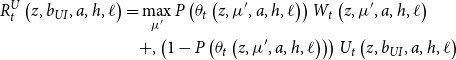
 \begin{equation} h' = e^{\epsilon'}\left (h + H\left (h,\ell, \tau \right )\right ), \end{equation}
where $H$
is a non-decreasing function of
$H$
is a non-decreasing function of $h$
,
$h$
, $\ell$
and
$\ell$
and $\tau$
; and
$\tau$
; and $\epsilon' \sim N\left (\mu _{\epsilon }^e,\sigma _{\epsilon }^e\right )$
is an i.i.d. shock to human capital. The unemployed do not accumulate human capital, but still face stochastic shocks, so that
$\epsilon' \sim N\left (\mu _{\epsilon }^e,\sigma _{\epsilon }^e\right )$
is an i.i.d. shock to human capital. The unemployed do not accumulate human capital, but still face stochastic shocks, so that
 \begin{equation} h' = e^{\epsilon^{\prime}}h, \end{equation}
where $\epsilon' \sim N\left (\mu _{\epsilon }^u,\sigma _{\epsilon }^u\right )$
. The human capital shock distribution for the unemployed is allowed to be different from that for the employed, to capture human capital depreciation during unemployment.
$\epsilon' \sim N\left (\mu _{\epsilon }^u,\sigma _{\epsilon }^u\right )$
. The human capital shock distribution for the unemployed is allowed to be different from that for the employed, to capture human capital depreciation during unemployment.
An unemployed worker receives unemployment benefit $b_{UI}$
if eligible for UI and a subsistence benefit
$b_{UI}$
if eligible for UI and a subsistence benefit $b_{L}\leq b_{UI}$
if ineligible. The amount
$b_{L}\leq b_{UI}$
if ineligible. The amount $b_{UI}$
is assumed to be a function of the worker’s last wage when employed. Specifically,
$b_{UI}$
is assumed to be a function of the worker’s last wage when employed. Specifically, $b_{UI} = \min \{\max \{bw,b_{L}\},\bar {b}\}$
, where
$b_{UI} = \min \{\max \{bw,b_{L}\},\bar {b}\}$
, where $w$
is the worker’s previous wage,
$w$
is the worker’s previous wage, $b$
is the replacement rate of unemployment insurance, and
$b$
is the replacement rate of unemployment insurance, and $\bar {b}$
is a cap on unemployment benefits. In other words, consistent with the actual UI system, unemployment benefits equal a fraction of the previous wage up to a maximum. An unemployed worker eligible for UI stochastically loses eligibility with probability
$\bar {b}$
is a cap on unemployment benefits. In other words, consistent with the actual UI system, unemployment benefits equal a fraction of the previous wage up to a maximum. An unemployed worker eligible for UI stochastically loses eligibility with probability $\gamma$
and regains eligibility upon becoming employed.
$\gamma$
and regains eligibility upon becoming employed.
Workers are allowed to smooth consumption over the life-cycle by borrowing and saving at exogenous rate $r_{F}$
. Workers are not allowed to default on debt obligations or exit the terminal period with negative asset holdings; we ensure this by assuming an age-dependent borrowing constraint
$r_{F}$
. Workers are not allowed to default on debt obligations or exit the terminal period with negative asset holdings; we ensure this by assuming an age-dependent borrowing constraint $\underline {a}'_t$
at each working age
$\underline {a}'_t$
at each working age $t$
. In retirement, workers may save, but are unable to borrow.
$t$
. In retirement, workers may save, but are unable to borrow.
There is a continuum of infinitely-lived risk-neutral firms, who discount the future with the same factor $\beta$
as workers. Firms post vacancies at cost
$\beta$
as workers. Firms post vacancies at cost $\kappa$
. Posted vacancies specify the piece rate wage
$\kappa$
. Posted vacancies specify the piece rate wage $\mu$
paid as earnings; the piece rate is restricted to be fixed for the duration of the contract. Search is directed, so that firms open vacancies for specific submarkets indexed by the characteristics of the workers. Each submarket is therefore identified by a tuple
$\mu$
paid as earnings; the piece rate is restricted to be fixed for the duration of the contract. Search is directed, so that firms open vacancies for specific submarkets indexed by the characteristics of the workers. Each submarket is therefore identified by a tuple $\left (\mu, a, h, \ell, t\right )$
. Once matched with a worker, a firm receives
$\left (\mu, a, h, \ell, t\right )$
. Once matched with a worker, a firm receives $\left (1 - \mu \right )\left (1 - \tau \right )zh$
in profits each period. The match dissolves either through exogenous separation or through the worker’s on-the-job search.
$\left (1 - \mu \right )\left (1 - \tau \right )zh$
in profits each period. The match dissolves either through exogenous separation or through the worker’s on-the-job search.
Matching in each submarket is characterized by a constant returns to scale matching function, $M\left (s, v\right )$
, where
$M\left (s, v\right )$
, where $s$
is the number of searchers in the submarket and
$s$
is the number of searchers in the submarket and $v$
is the number of posted vacancies in the submarket. Define the submarket tightness
$v$
is the number of posted vacancies in the submarket. Define the submarket tightness $\theta =v/s$
to be the vacancy-worker ratio in each submarket. Firms meet workers with probability
$\theta =v/s$
to be the vacancy-worker ratio in each submarket. Firms meet workers with probability $q\left (\theta \right ) = \frac {M\left (s, v\right )}{v}$
, which is twice continuously differentiable and strictly decreasing, and bounded between 0 and 1; workers meet firms with probability
$q\left (\theta \right ) = \frac {M\left (s, v\right )}{v}$
, which is twice continuously differentiable and strictly decreasing, and bounded between 0 and 1; workers meet firms with probability $p\left (\theta \right ) = \theta q\left (\theta \right ) = \frac {M\left (s, v\right )}{s}$
, which is twice continuously differentiable, strictly increasing and strictly concave, and likewise bounded between 0 and 1. We will denote the tightness in submarket
$p\left (\theta \right ) = \theta q\left (\theta \right ) = \frac {M\left (s, v\right )}{s}$
, which is twice continuously differentiable, strictly increasing and strictly concave, and likewise bounded between 0 and 1. We will denote the tightness in submarket $\left (\mu, a, h, \ell, t\right )$
by
$\left (\mu, a, h, \ell, t\right )$
by $\theta _{t}\left (\mu, a, h, \ell \right )$
.
$\theta _{t}\left (\mu, a, h, \ell \right )$
.
The aggregate productivity shocks $z$
evolve according to
$z$
evolve according to
 \begin{equation} \ln z' = \rho _{z}\ln z + \epsilon _{z}', \quad \text{where} \quad \epsilon _{z}'\sim N\left (\mu _{z},\sigma _{z}\right ). \end{equation}
The aggregate state of the economy consists of the aggregate productivity level $z$
as well as the distribution of workers across idiosyncratic characteristics. Following Menzio and Shi (Reference Menzio and Shi2011), we focus on block recursive equilibrium (BRE), in which decision rules depend on the aggregate state only through aggregate productivity
$z$
as well as the distribution of workers across idiosyncratic characteristics. Following Menzio and Shi (Reference Menzio and Shi2011), we focus on block recursive equilibrium (BRE), in which decision rules depend on the aggregate state only through aggregate productivity $z$
, but do not depend on the distribution of workers.
$z$
, but do not depend on the distribution of workers.
2.2 Worker’s problem
2.2.1 Production, savings, and human capital accumulation
Each period is divided into two stages: job search and production. During the production stage, workers choose consumption and savings allocations, and employed workers additionally choose the proportion of time spent accumulating human capital. Following these decisions, age advances, workers receive human capital shocks, and unemployment insurance benefits stochastically expire.
The problem of an unemployed worker eligible for unemployment insurance is given by
 \begin{align} U_{t}\left (z, b_{UI}, a, h, \ell \right ) &= \max _{c, a'\geq -\underline {a}'_t} u\left (c\right ) + \beta \mathbb{E}[\left (1 - \gamma \right )R_{t + 1}^{U}\left (z', b_{UI}, a', h', \ell \right ) + \gamma R_{t + 1}^{U}\left (z', b_{L}, a', h', \ell \right )] \end{align}
 \begin{align} \text{s.t. } c + a' &\leq \left (1 + r_{F}\right )a + b_{UI} \end{align}
 \begin{align} h' &= e^{\epsilon'}h, \text{ where } \epsilon' \sim N\left (\mu _{\epsilon }^u,\sigma _{\epsilon }^u\right ) \end{align}
 \begin{align} \ln z' &= \rho _{z}\ln z + \epsilon _{z}', \text{ where }\epsilon _{z}'\sim N\left (\mu _{z},\sigma _{z}\right ) \end{align}
Unemployed agents stochastically lose their benefits with probability $\gamma$
, and face shocks
$\gamma$
, and face shocks $\epsilon'$
to their human capital, both realized at the beginning of the search period. Unemployed agents without unemployment insurance face a similar problem:
$\epsilon'$
to their human capital, both realized at the beginning of the search period. Unemployed agents without unemployment insurance face a similar problem:
 \begin{align} U_{t}\left (z, b_{L}, a, h, \ell \right ) &= \max _{c, a'\geq -\underline {a}'_t} u\left (c\right ) + \beta \mathbb{E}[R_{t + 1}^{U}\left (z', b_{L}, a', h', \ell \right )] \end{align}
 \begin{align} \text{s.t. } c + a' &\leq \left (1 + r_{F}\right )a + b_{L} \end{align}
 \begin{align} h' &= e^{\epsilon'}h, \text{ where } \epsilon '\sim N\left (\mu _{\epsilon }^u,\sigma _{\epsilon }^u\right ) \end{align}
 \begin{align} \ln z' &= \rho _{z}\ln z + \epsilon _{z}', \text{ where }\epsilon _{z}'\sim N\left (\mu _{z},\sigma _{z}\right ) \end{align}
Once an unemployed worker loses UI eligibility, they must become employed again to regain it.
The problem of an employed worker is:
 \begin{align} W_{t} (z, \mu, a, h, \ell ) & = \! \max _{c, a'\geq -\underline {a}'_t, \tau \in [0,1]} u (c) + \beta \mathbb{E} \left[(1 - \delta )R_{t + 1}^{E} (z', \mu, a', h', \ell ) + \delta R_{t + 1}^{U} (z', b_{UI}, a', h', \ell )\right] \end{align}
 \begin{align} \text{s.t. } c + a' &\leq \left (1 + r_{F}\right )a + \mu \left (1 - \tau \right )f\left (z,h\right ) \end{align}
 \begin{align} h' &= e^{\epsilon '}\left (h + H\left (h, \ell, \tau \right )\right ), \text{ where } \epsilon '\sim N\left (\mu _{\epsilon }^e,\sigma _{\epsilon }^e\right ) \end{align}
 \begin{align} b_{UI} &= \min \{\max \{b\left (1 - \tau \right )\mu zh,b_{L}\},\bar {b}\} \end{align}
 \begin{align} \ln z' &= \rho _{z}\ln z + \epsilon _{z}', \text{ where }\epsilon _{z}'\sim N\left (\mu _{z},\sigma _{z}\right ) \end{align}
Newly unemployed agents are assumed to be eligible UI benefits, which are determined by a replacement rate $b$
of previous wages and capped at
$b$
of previous wages and capped at $\bar {b}$
.
$\bar {b}$
.
2.2.2 Job search
Age advances and shocks are realized following the production period. Unemployed agents in the job search period choose the piece-rate $\mu '$
the apply to by solving the problem given by Equation 2.17:
$\mu '$
the apply to by solving the problem given by Equation 2.17:
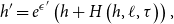
 \begin{align} \nonumber R_{t}^{U}\left (z, b_{UI}, a, h, \ell \right ) &=\max _{\mu '}P\left (\theta _{t}\left (z, \mu ', a, h, \ell \right )\right )W_{t}\left (z, \mu ', a, h, \ell \right )\\ &\quad +, \left (1 - P\left (\theta _{t}\left (z, \mu ', a, h, \ell \right )\right )\right )U_{t}\left (z, b_{UI}, a, h, \ell \right ) \end{align}
For agents without unemployment insurance, the problem is identical except that $b_{UI}$
is replaced by
$b_{UI}$
is replaced by $ b_{L}$
. Employed workers are allowed to search on the job, and solve the problem given by Equation 2.18:
$ b_{L}$
. Employed workers are allowed to search on the job, and solve the problem given by Equation 2.18:
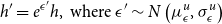
 \begin{align} \nonumber R_{t}^{E}\left (z, \mu, a, h, \ell \right ) &= \max _{\mu '}\lambda _{E}P\left (\theta _{t}\left (z, \mu ', a, h, \ell \right )\right )W_{t}\left (z, \mu ', a, h, \ell \right )\\ &\quad +\, \left (1 - \lambda _{E}P\left (\theta _{t}\left (z, \mu ', a, h, \ell \right )\right )\right )W_{t}\left (z, \mu, a, h, \ell \right ) \end{align}
2.3 Firm’s problem
Firms produce using a single worker as an input. They post piece-rate wage contracts in submarkets indexed by $\left (z, \mu, a, h, \ell, t\right )$
.
$\left (z, \mu, a, h, \ell, t\right )$
.
With probability $\left (1 - \delta \right )\left (1 - \lambda _{E}P\left (\left (\theta _{t + 1}\left (z, \mu ', a', h', \ell \right )\right )\right )\right )$
, the match does not separate exogenously and the worker does not find a new employer. The value function of a firm matched with a worker is given in Equation 2.19:
$\left (1 - \delta \right )\left (1 - \lambda _{E}P\left (\left (\theta _{t + 1}\left (z, \mu ', a', h', \ell \right )\right )\right )\right )$
, the match does not separate exogenously and the worker does not find a new employer. The value function of a firm matched with a worker is given in Equation 2.19:
 \begin{align} J_{t} (z, \mu, a, h, \ell ) &= (1 - \mu ) (1 - \tau )zh+ \beta E \left[ (1 - \delta ) (1 - \lambda _{E}P (\theta _{t + 1} (\mu ', a', h', \ell ) ) ) J_{t + 1} (\mu, a', h', \ell )\right], \end{align}
where $h'$
evolves according to (2.14),
$h'$
evolves according to (2.14), $a' = g_{a}\left (z, \mu, a, h, \ell \right )$
and
$a' = g_{a}\left (z, \mu, a, h, \ell \right )$
and $\tau = g_{\tau }\left (z, \mu, a, h, \ell \right )$
are the worker policy decisions over wealth and human capital accumulation, and
$\tau = g_{\tau }\left (z, \mu, a, h, \ell \right )$
are the worker policy decisions over wealth and human capital accumulation, and $\mu ' = g_{\mu '}\left (z, \mu, a', h', \ell \right )$
is the on-the-job application strategy of the worker conditional upon his asset and human capital policy rule. New firms have the option of posting a vacancy at cost
$\mu ' = g_{\mu '}\left (z, \mu, a', h', \ell \right )$
is the on-the-job application strategy of the worker conditional upon his asset and human capital policy rule. New firms have the option of posting a vacancy at cost $\kappa$
in any submarket. Each submarket offers a probability of matching with a worker given by
$\kappa$
in any submarket. Each submarket offers a probability of matching with a worker given by $q\left (\theta _{t}\left (z, \mu, a, h, \ell \right )\right )$
. By free entry the value of a vacancy is zero, and we have
$q\left (\theta _{t}\left (z, \mu, a, h, \ell \right )\right )$
. By free entry the value of a vacancy is zero, and we have
 \begin{equation} \kappa = q\left (\theta _{t}\left (z, \mu, a, h, \ell \right )\right )J_{t}\left (z, \mu, a, h, \ell \right ) \end{equation}
This free entry condition determines $\theta _t\left (z, \mu, a, h, l\right )$
.
$\theta _t\left (z, \mu, a, h, l\right )$
.
2.4 Equilibrium
A BRE in this model economy is a set of policy functions for workers, $\{c, \mu ', a', \tau \}$
, value functions for workers
$\{c, \mu ', a', \tau \}$
, value functions for workers $W_{t}, U_{t}$
, value functions for firms
$W_{t}, U_{t}$
, value functions for firms $J_{t}$
, as well as a market tightness function
$J_{t}$
, as well as a market tightness function $\theta _{t}\left (z, \mu, a, h, \ell \right )$
, that satisfy the following:
$\theta _{t}\left (z, \mu, a, h, \ell \right )$
, that satisfy the following:
-
1. The policy functions $\{c, \mu ', a', \tau \}$
solve the workers problems,
$W_{t}, U_{t}, R_{t}^{E}, R_{t}^{U}$
.
$\{c, \mu ', a', \tau \}$
solve the workers problems,
$W_{t}, U_{t}, R_{t}^{E}, R_{t}^{U}$
. -
2.
$\theta _{t}\left (z, \mu, a, h, \ell \right )$
satisfies the free entry condition for all submarkets
$\left (z,\mu, a, h, \ell, t\right )$
. -
3. The aggregate law of motion is consistent with all policy functions.


3. Estimation
Before describing our calibration procedure in detail, we lay out the overall estimation strategy and the intuition for identification of key parameters. The centerpiece of the calibration is identifying the joint distribution of initial conditions, which consist of wealth, human capital, and learning ability, together with the human capital production technology and the the matching technology. Since initial wealth observed directly, the marginal distribution of initial wealth is identified from initial wealth data. Next, both learning ability and the human capital production technology $\alpha$
affect the life-cycle earnings profile. To separately identify them, we target both the slope and the curvature of the earnings profile. We then target the earnings variance profile to discipline the dispersion of learning ability. Finally, the distribution of initial human capital is identified from the distribution of initial earnings. The non-trivial aspect of this is that workers are not paid their marginal product. However, the structure of the model disciplines the distribution of accepted piece rates, given other parameters, in particular the elasticity of the matching technology and the level of subsistence consumption. Intuitively, the subsistence level of consumption affects how selective workers of different wealth levels are in choosing what piece rates to apply for; in turn, the elasticity of the matching function governs the mapping between piece-rates and job finding probabilities. Therefore, we also target the distribution of job-to-job transition rates by wealth and the distribution earnings changes from job-to-job transitions by wealth to identify these two parameters.
$\alpha$
affect the life-cycle earnings profile. To separately identify them, we target both the slope and the curvature of the earnings profile. We then target the earnings variance profile to discipline the dispersion of learning ability. Finally, the distribution of initial human capital is identified from the distribution of initial earnings. The non-trivial aspect of this is that workers are not paid their marginal product. However, the structure of the model disciplines the distribution of accepted piece rates, given other parameters, in particular the elasticity of the matching technology and the level of subsistence consumption. Intuitively, the subsistence level of consumption affects how selective workers of different wealth levels are in choosing what piece rates to apply for; in turn, the elasticity of the matching function governs the mapping between piece-rates and job finding probabilities. Therefore, we also target the distribution of job-to-job transition rates by wealth and the distribution earnings changes from job-to-job transitions by wealth to identify these two parameters.
3.1 Functional forms and distributional assumptions
Worker utility is of the constant relative risk aversion form:
 \begin{equation} u\left (c\right ) = \frac {c^{1 - \sigma } - 1}{1 - \sigma } \end{equation}
We use the matching function assumed by den Haan et al. (Reference den, Wouter, Ramey and Watson2000), which guarantees well-defined probabilities:
 \begin{align} M\left (u, v\right ) &= \frac {uv}{\left (u^{\eta } + v^{\eta }\right )^{\frac {1}{\eta }}} \end{align}
The human capital accumulation technology takes the form
 \begin{equation} H(h, \ell, \tau ) = \ell \left (h\tau \right )^{\alpha },\quad {}\alpha \gt 0 \end{equation}
To rule out negative asset holdings in the terminal period, the age-dependent borrowing limit is set to the maximum amount a worker could repay if they experienced the worst-possible sequence of shocks up to retirement:
 \begin{align} \underline {a}_{t}' = \sum _{j = t}^{T}\frac {b_{L}}{(1 + r_{F})^{j}} \end{align}
Initial conditions $(a_{0}, h_{0}, \ell )$
are drawn from a trivariate log-normal distribution with mean
$(a_{0}, h_{0}, \ell )$
are drawn from a trivariate log-normal distribution with mean $\psi$
and variance-covariance
$\psi$
and variance-covariance $\Sigma$
. We allow for correlations between each marginal distribution using a Gaussian Copula. We also allow each marginal distribution to be “displaced” by constant,
$\Sigma$
. We allow for correlations between each marginal distribution using a Gaussian Copula. We also allow each marginal distribution to be “displaced” by constant, $-\underline {a}_{0}, h_{min}$
, and
$-\underline {a}_{0}, h_{min}$
, and $\ell _{min}$
, for wealth, human capital, and learning ability, respectively. Subtracting the initial borrowing constraint allows workers to enter the labor market with debt, while
$\ell _{min}$
, for wealth, human capital, and learning ability, respectively. Subtracting the initial borrowing constraint allows workers to enter the labor market with debt, while $h_{min}$
and
$h_{min}$
and $\ell _{min}$
ensure that all workers experience positive earnings and human capital growth.
$\ell _{min}$
ensure that all workers experience positive earnings and human capital growth.
3.2 Preset parameter values
The model period is a quarter, and agents live for $T = 168$
quarters. We set the minimum age in the model to 23, implying that the model covers ages 23–65. We choose the separation rate to match quarterly flows from employment to unemployment in Shimer (Reference Shimer2012),
$T = 168$
quarters. We set the minimum age in the model to 23, implying that the model covers ages 23–65. We choose the separation rate to match quarterly flows from employment to unemployment in Shimer (Reference Shimer2012), $\delta = 0.03$
. We set the quarterly interest rate to equal an annual rate of approximately 5% (
$\delta = 0.03$
. We set the quarterly interest rate to equal an annual rate of approximately 5% ( $r_{F} = 0.012$
) which is roughly its value for much of the period over which our model is calibrated, and set
$r_{F} = 0.012$
) which is roughly its value for much of the period over which our model is calibrated, and set $\beta = \frac {1}{1 + r_{F}}$
. The risk aversion parameter is set to a standard value
$\beta = \frac {1}{1 + r_{F}}$
. The risk aversion parameter is set to a standard value $\sigma =2$
. The average income of an employed 25-year old worker is normalized to 1.
$\sigma =2$
. The average income of an employed 25-year old worker is normalized to 1.
We calibrate the unemployment insurance system to closely resemble the system in the US prior to the Great Recession. We set the unemployment insurance replacement rate to its average in the data, $b = 0.42$
, and cap unemployment insurance at a weekly maximum of
$b = 0.42$
, and cap unemployment insurance at a weekly maximum of $\bar {b}=\$900$
, which is comparable to the higher caps on UI in the US. We assume that unemployment insurance can be lost stochastically with probability
$\bar {b}=\$900$
, which is comparable to the higher caps on UI in the US. We assume that unemployment insurance can be lost stochastically with probability $\gamma = 0.54$
, which matches the average weeks until expiration (
$\gamma = 0.54$
, which matches the average weeks until expiration ( $\approx 24.1$
weeks) for a new UI recipient in the US. We also set the retirement income to
$\approx 24.1$
weeks) for a new UI recipient in the US. We also set the retirement income to $b_{Ret}$
to the average Social Security income. We set the mortality rate after retirement to the US average after the age of 66,
$b_{Ret}$
to the average Social Security income. We set the mortality rate after retirement to the US average after the age of 66, $\delta _{D} = 0.02$
per quarter.
$\delta _{D} = 0.02$
per quarter.
3.3 Internally calibrated parameters
The remaining parameters are estimated using indirect inference, using a strategy similar (but not identical) to Griffy (Reference Griffy2021). We target parameters other than the aggregate productivity process in the steady state; conditional on these estimates, we calibrate the productivity process to match the persistence and volatility of output per worker.
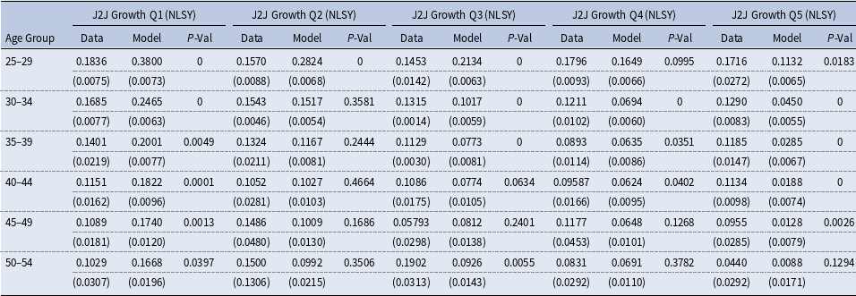
We target the unconditional distribution of initial net liquid wealth and the unconditional distribution of initial earnings at first employment, both drawn from the Panel Study of Income Dynamics (PSID). Matching the initial wealth distribution in the data identifies parameters from the marginal distribution of initial wealth in the model. Matching the initial earnings distribution in the data identifies the marginal distribution of initial human capital. Note that earnings do not equal human capital in the model, but the structure of the model puts discipline on the mapping between the two, through endogenous choice of piece rates and productive time. We also target the life-cycle earnings profile and the life-cycle variance profile to identify the human capital accumulation technology and the marginal distribution of learning ability. Intuitively, the life-cycle earnings profile identifies both the mean learning ability and the curvature parameter $\alpha$
of the human capital technology. The reason that mean learning ability and
$\alpha$
of the human capital technology. The reason that mean learning ability and $\alpha$
are separately identified is that the former affects earnings growth linearly, while the latter affects it non-linearly; they are thus jointly identified by the average earnings growth and the curvature of the earnings profile. In turn, the variance of learning ability is identified by the life-cycle profile of earnings variance: intuitively, if learning ability is more dispersed, then earnings variance increases more with age. To discipline the correlations between initial conditions, we target two Mincer regressions in which the slope and intercept are interacted with a worker’s initial wealth or learning ability quintile.Footnote 2 This identifies the correlations between initial wealth, initial human capital, and initial learning ability (
$\alpha$
are separately identified is that the former affects earnings growth linearly, while the latter affects it non-linearly; they are thus jointly identified by the average earnings growth and the curvature of the earnings profile. In turn, the variance of learning ability is identified by the life-cycle profile of earnings variance: intuitively, if learning ability is more dispersed, then earnings variance increases more with age. To discipline the correlations between initial conditions, we target two Mincer regressions in which the slope and intercept are interacted with a worker’s initial wealth or learning ability quintile.Footnote 2 This identifies the correlations between initial wealth, initial human capital, and initial learning ability ( $\rho _{AH}, \rho _{A\ell }, \rho _{H\ell }$
), which are estimated using a Gaussian Copula.Footnote 3
$\rho _{AH}, \rho _{A\ell }, \rho _{H\ell }$
), which are estimated using a Gaussian Copula.Footnote 3
Our model allows for shocks to human capital, which are further allowed to differ by employment status. To discipline these parameters ( $\mu _{\epsilon _{E}}$
,
$\mu _{\epsilon _{E}}$
, $\sigma _{\epsilon _{E}}$
,
$\sigma _{\epsilon _{E}}$
, $\mu _{\epsilon _{U}}$
,
$\mu _{\epsilon _{U}}$
, $\sigma _{\epsilon _{U}}$
), we modify the identification strategy used by Huggett et al. (Reference Huggett, Ventura and Yaron2011). Specifically, we target earnings changes as workers approach retirement, and do so separately by employment status. Between periods, human capital may change due to investment or depreciation. As workers approach retirement they are less likely to invest in human capital, which means that observed changes in earnings are due to human capital depreciation. Because we would like to isolate human capital depreciation for the employed and unemployed separately, we focus on earnings changes between ages-
$\sigma _{\epsilon _{U}}$
), we modify the identification strategy used by Huggett et al. (Reference Huggett, Ventura and Yaron2011). Specifically, we target earnings changes as workers approach retirement, and do so separately by employment status. Between periods, human capital may change due to investment or depreciation. As workers approach retirement they are less likely to invest in human capital, which means that observed changes in earnings are due to human capital depreciation. Because we would like to isolate human capital depreciation for the employed and unemployed separately, we focus on earnings changes between ages- $t-1$
and
$t-1$
and $t+n-1$
and use employment status at age-
$t+n-1$
and use employment status at age- $t$
.
$t$
.
Table 1. Preset parameter values
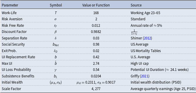
Table 2. Estimated parameters
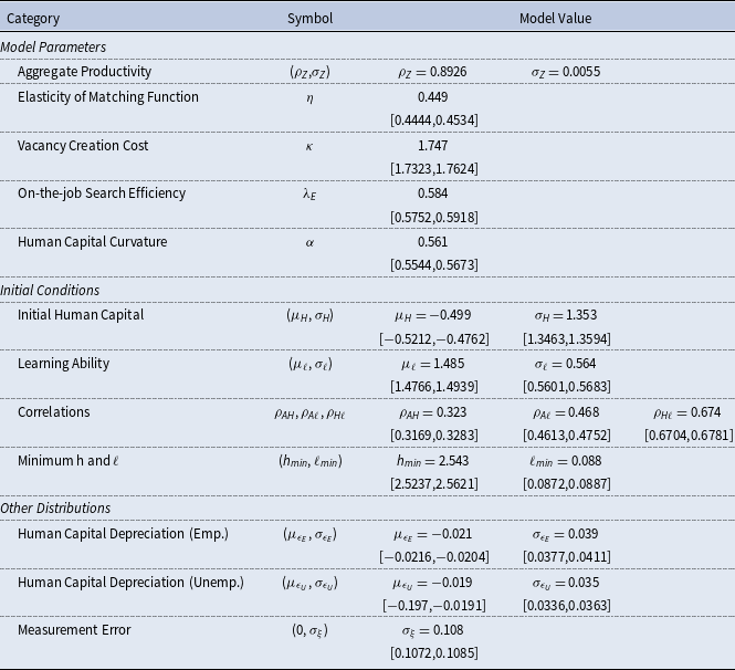
Note: The 95% confidence intervals of the estimates are shown in brackets beneath the structural parameters.
Table 3. Aggregate moments: labor productivity
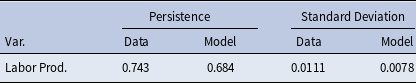
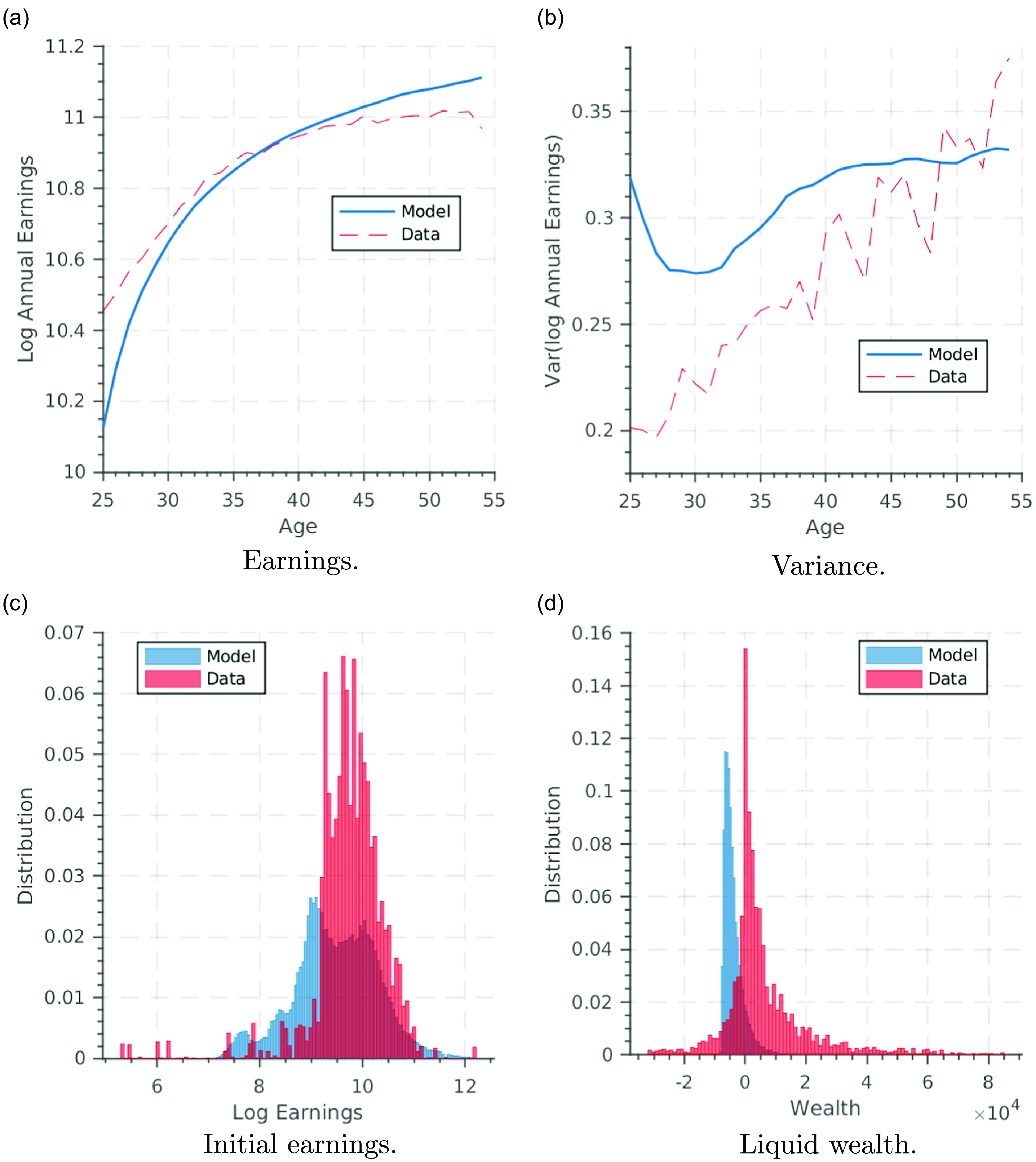
Figure 1. Model fit.
3.4 Estimation results and model fit
The parameter estimates are reported in Table 1 and Table 2. The estimation results of the auxiliary model are reported in Table 3, Table 8, Table 9. and Table 10. Despite having more than 200 auxiliary parameters, difference-in-means tests show that the model replicates the data along many dimensions. The model comes reasonably close to replicating the average earnings profile (Figure 1a), but overestimates the variance profile, despite capturing the overall shape (Figure 1b). The model also matches the initial distribution of earnings (Figure 1c) as well as the initial distribution of wealth (Figure 1d).
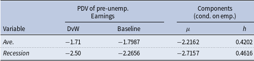
As an additional validation test, we compare our findings to the empirical results of Davis and von Wachter (Reference Davis and von Wachter2011) on the earnings costs of displacement. We focus on the average cost of displacement, and the cost of displacement during a recession, and calculate the earnings losses relative to their pre-displacement level. We present our results in Table 4, as well as the contribution of each component of income in our model, $\mu$
and
$\mu$
and $h$
.
$h$
.
We find that our model does a reasonable job replicating the magnitude of earnings losses on average, but understates the loss that results from a recesssion by roughly 25pp. Still, this provides an endorsement of the mechanism present in the model, where those who lose their job during a recession face a substantially weaker labor market. We provide a decomposition of the contributions of different components in Table 11.
4. Results
4.1 The impact of an aggregate productivity shock
We now assess the effects of a recession on aggregate human capital, productivity, and unemployment, and then explore the mechanisms driving these effects. To do so, we assume that the economy is struck by a 6 quarter downturn of 3.5%, after which productivity returns to the steady-state at a rate of $z_{t + 1} = \rho z_{t}$
. We assume that the economy was initially in steady state.
$z_{t + 1} = \rho z_{t}$
. We assume that the economy was initially in steady state.
Table 4. Comparison with Davis von Wachter (2011)
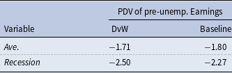
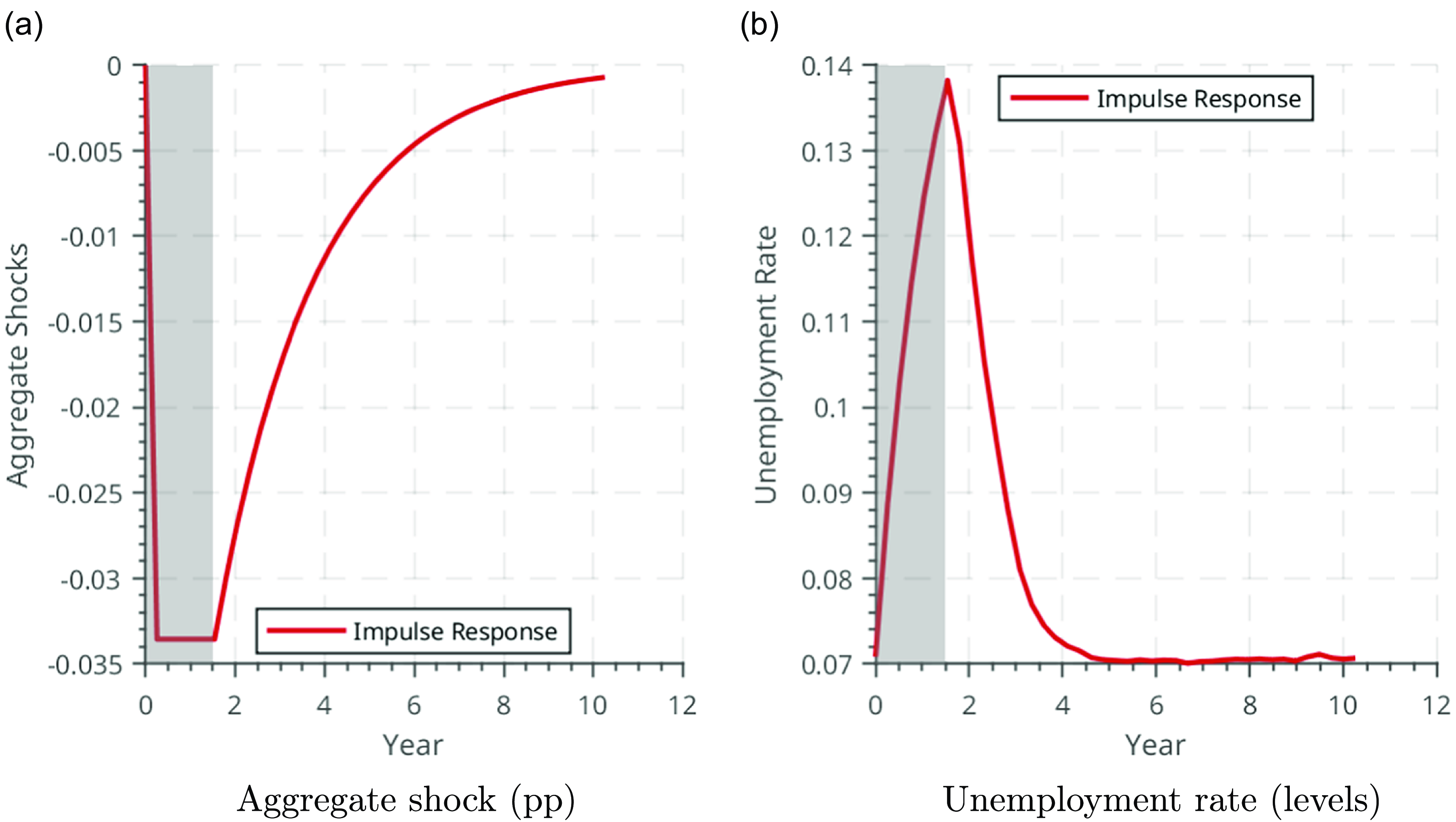
Figure 2. Effect of a negative productivity shock: unemployment.
Figure 2 shows the path of the exogenous shock $z_t$
(in panel 2a) and the resulting path of the unemployment rate (in panel 2b). The recession leads to a large increase and gradual recovery in unemployment. Figure 3 shows the corresponding paths of output (panel 3a), output per worker (panel 3b), and the average human capital of employed workers (panel 3c). The fall in output per worker is more persistent than the shock itself, due to the decline in average human capital. Notably, as shown in panel 3c, average human capital per employed worker rises during the period of the recession but then exhibits a persistent decline during the recovery. Table 5 illustrates a similar point by comparing the changes in key aggregates, relative to steady state, 6 quarters and 40 quarters after the initial shock. While output and earnings recover, the fall in average human capital is persistent. The subsequent figures explore why this is the case.
$z_t$
(in panel 2a) and the resulting path of the unemployment rate (in panel 2b). The recession leads to a large increase and gradual recovery in unemployment. Figure 3 shows the corresponding paths of output (panel 3a), output per worker (panel 3b), and the average human capital of employed workers (panel 3c). The fall in output per worker is more persistent than the shock itself, due to the decline in average human capital. Notably, as shown in panel 3c, average human capital per employed worker rises during the period of the recession but then exhibits a persistent decline during the recovery. Table 5 illustrates a similar point by comparing the changes in key aggregates, relative to steady state, 6 quarters and 40 quarters after the initial shock. While output and earnings recover, the fall in average human capital is persistent. The subsequent figures explore why this is the case.
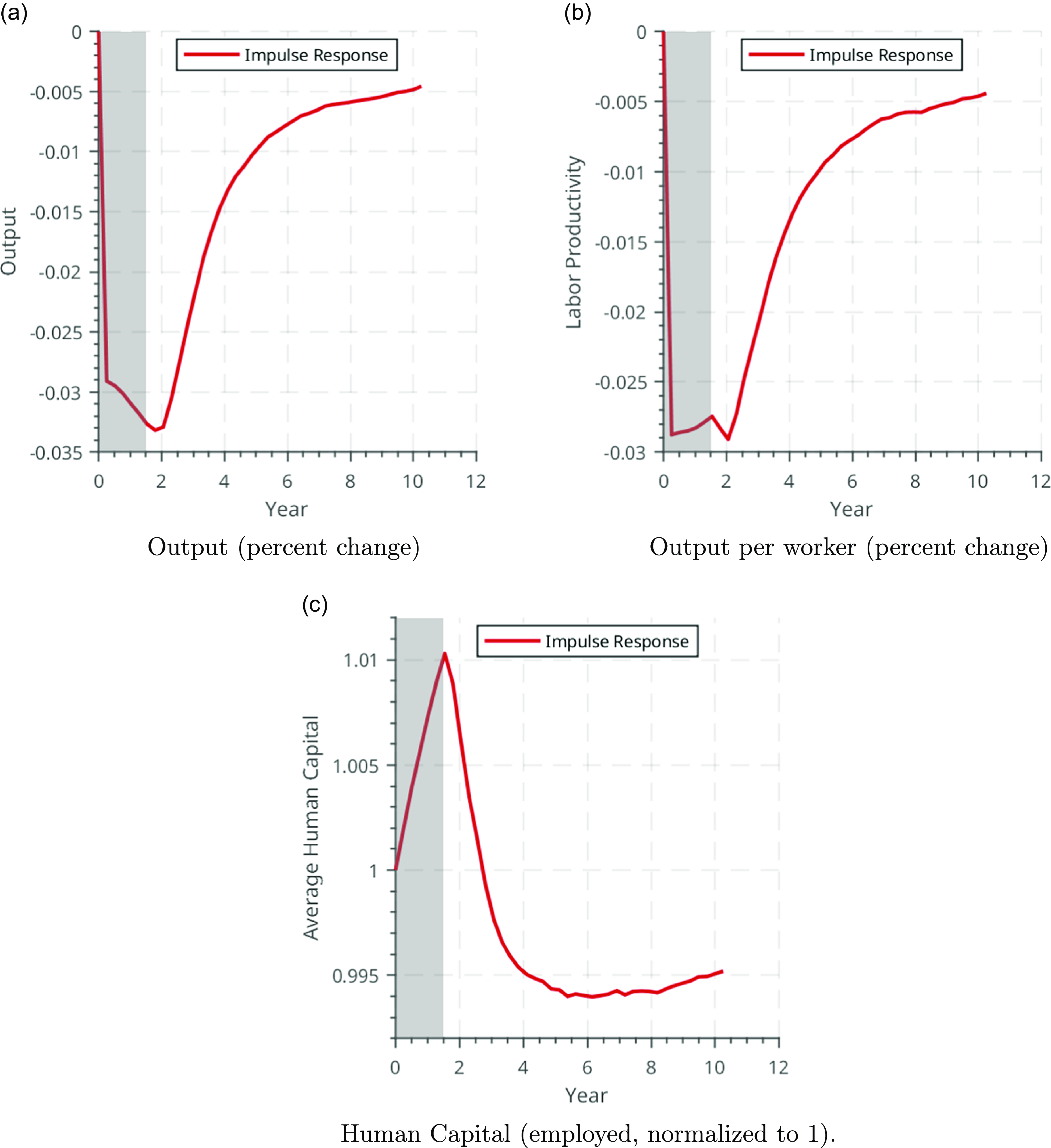
Figure 3. Effect of a negative productivity shock: output and average human capital.
Figure 4 illustrates how the key decisions of the unemployed and employed respond to the negative shock. Panel 4a shows that the average piece rate, $\mu$
, exhibits a gradual decline. Panel 4b shows that, unsurprisingly, this is largely driven by a large change in the application strategies of the unemployed, who apply for lower piece rates. At the same time, they remain unemployed for longer on average, as shown in panel 4c. These results are consistent with the theoretical predictions of a canonical directed search model, in which a drop in aggregate productivity exacerbates the wage/job-finding tradeoff, leading to both lower targeted wages and a lower job-finding rate. Panel 4e plots the job-to-job transition rates through on-the-job search, showing that employed individuals also suffer a slowdown in the progression up the job ladder.
$\mu$
, exhibits a gradual decline. Panel 4b shows that, unsurprisingly, this is largely driven by a large change in the application strategies of the unemployed, who apply for lower piece rates. At the same time, they remain unemployed for longer on average, as shown in panel 4c. These results are consistent with the theoretical predictions of a canonical directed search model, in which a drop in aggregate productivity exacerbates the wage/job-finding tradeoff, leading to both lower targeted wages and a lower job-finding rate. Panel 4e plots the job-to-job transition rates through on-the-job search, showing that employed individuals also suffer a slowdown in the progression up the job ladder.
Table 5. Effects of a negative productivity shock
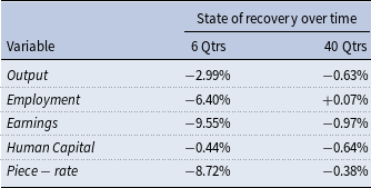
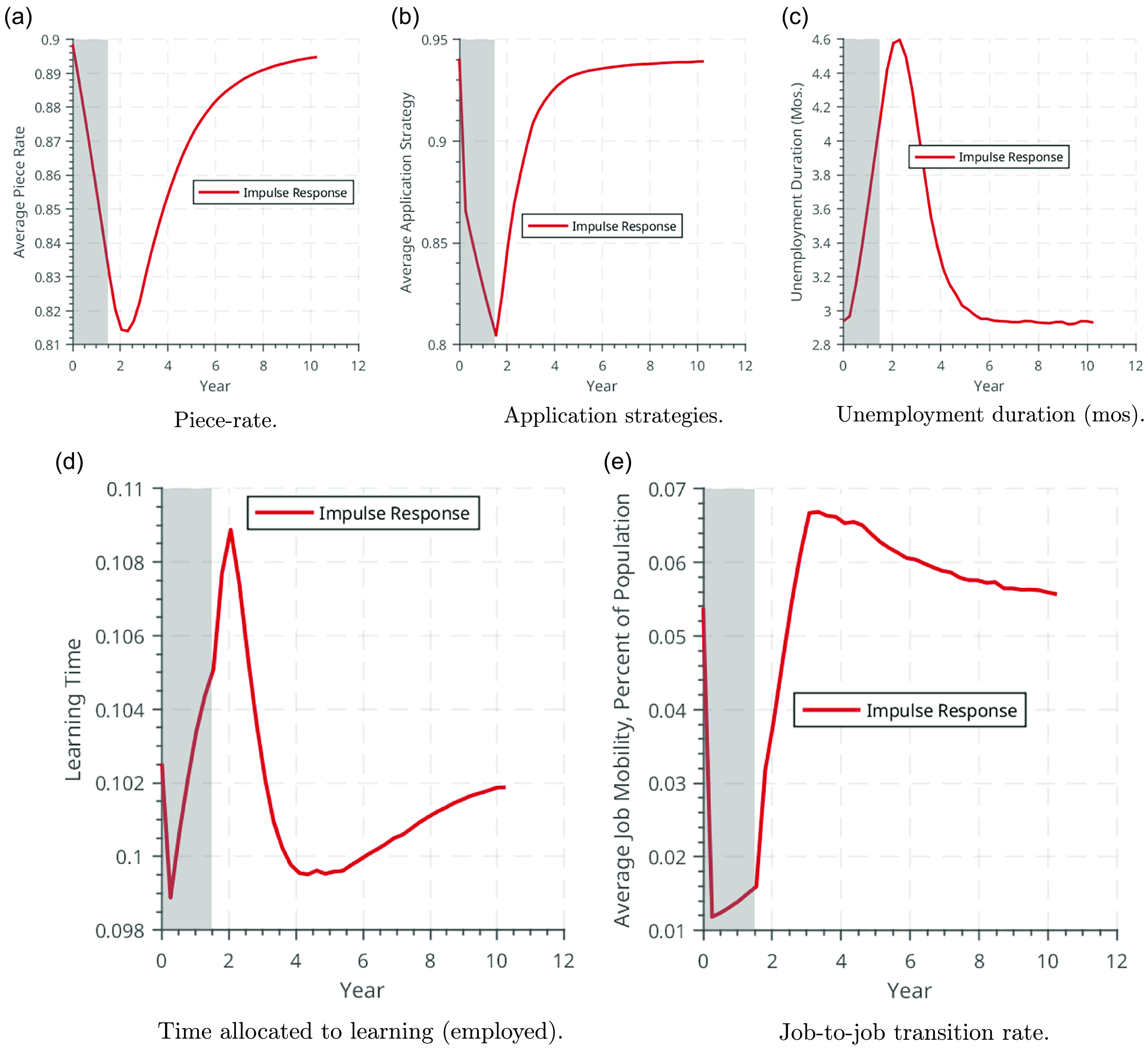
Figure 4. Effect of a negative productivity shock: search behavior and learning time.
Of particular interest is panel 4d, which shows the average learning time among the employed workers. Average learning time falls on impact, then exhibits a non-monotonic pattern. The fact that average learning time falls on impact in response to the shock but no such immediate fall is observed in average human capital in Figure 3c suggests that there are important composition effects driving the results. The negative aggregate shock leads to a “cleansing” effect: since unemployed workers with low human capital are less attractive to employers and have disproportionately low job-finding rates, the composition of the employment pool shifts toward workers of high human capital (indeed, the average human capital per worker in the population falls while average human capital per employed worker rises). Furthermore, as argued above, because wealth and age are correlated, the reduction in learning is concentrated among the poor and young workers, who—at the onset of the recession —account for only a small fraction of the employed and therefore of the average employed human capital.
Crucially, the fact that the drop in learning is concentrated among the young and poor, and that this drop appears temporary in Figure 4d, does not imply that this drop is unimportant for aggregate human capital dynamics: quite the opposite is true. This response is, in fact, critical for explaining the long-term decline in human capital in Figure 3c. Since the drop in human capital accumulation is concentrated among the young cohorts, these low human capital cohorts become progressively more important in the determination of the average human capital as the recession progresses. Moreover, as the aggregate shock recovers, the “cleansing” effect dissipates, and the low human-capital workers re-enter employment: the employment pool shifts toward workers who have lower human capital and are on persistently lower learning trajectories. This accounts for the eventual persistent drop in both average learning time (Figure 4d) and average human capital (Figure 3c). In other words, the interaction between heterogeneous responses and the composition of the employment pool is crucial for the propagation of the shock.
Last, we directly explore differences between cohorts. We examine a cohort who enters the labor market at the beginning of the recession and compare the impact on their lifetime earnings, placement, and human capital trajectories to a cohort who enters during the last quarter of the recession. We present each of these time series in Figure 5.
These figures demonstrate how severely a recession can impact new labor market entrants. While the final cohort who enters during a recession (the three right panels) experiences similar initial degrees of earnings loss, placement loss, and change in human capital, these losses dissipate more rapidly as the economy improves. The cohort who enters at the start of the recession (the left three panels) is left behind: while they entered the labor market prior to their younger peers, after 20 quarters, their younger peers are earning more, and are employed in jobs at higher rungs of the job ladder, despite having spent 6 fewer quarters in the labor market. The earlier entrants are also persistently behind their younger peers in terms of human capital. For long-exposed young cohorts, recessions cause palpable changes to their earnings trajectories. Crucially, these cohorts are young, only starting to invest in their future human capital, and have the least wealth to shield themselves against the downturn, leading to persistent effects. Similarly to Griffy (Reference Griffy2021), the persistent relative earnings loss of the older cohorts is primarily due to their failure to catch on human capital accumulation, relative to the younger ones. Note that these results are supported by empirical evidence (see, e.g., Kahn (Reference Kahn2010), Wee (Reference Wee2013), and Guo (Reference Guo2018)) that entering the labor market in a recession leads to persistent earnings losses relative to entering in a boom.
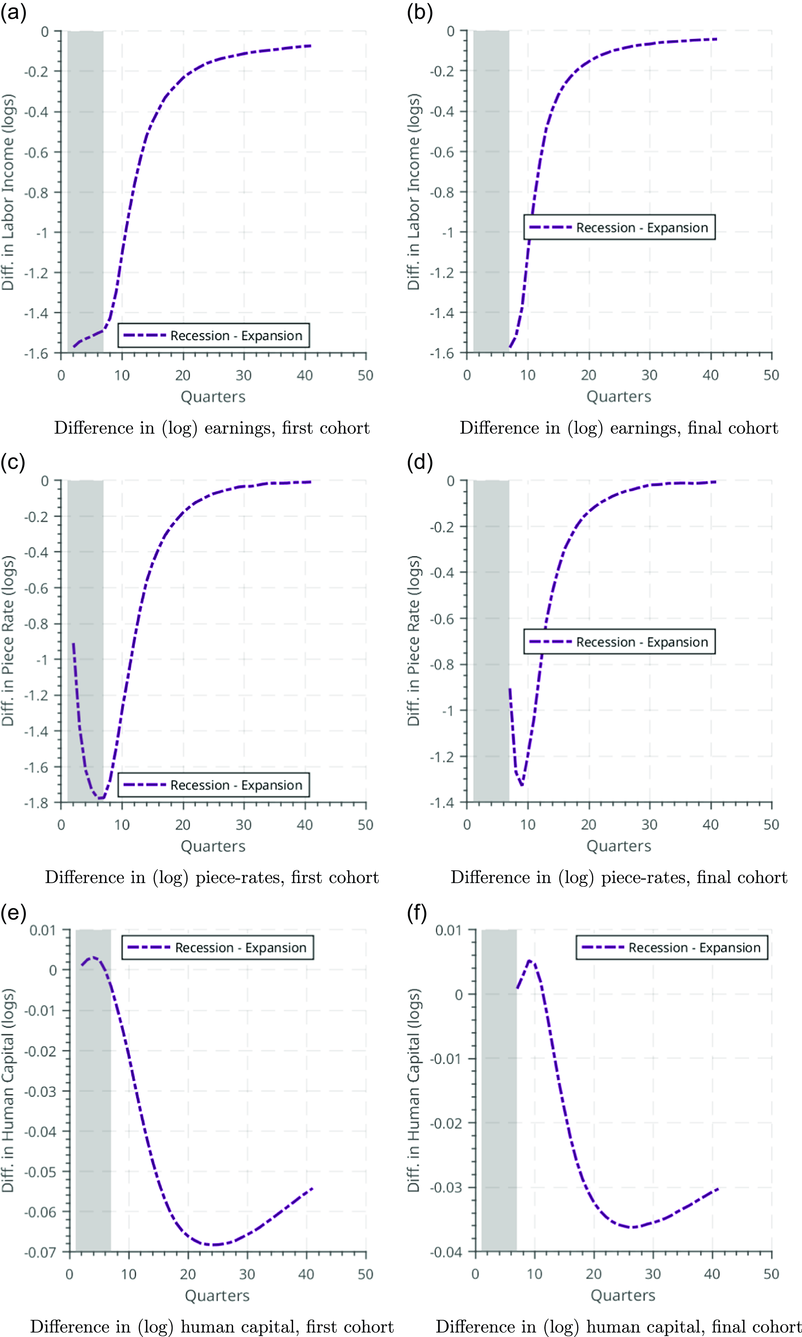
Figure 5. Impact of recession on key variables by cohort exposure to recession.
4.2 Differential effects by wealth
To further illustrate the mechanisms at play, we disaggregate the effects of a recession by wealth. As we will show, the aggregate results displayed above mask important heterogeneity in individual responses of human capital accumulation. This is because a decline in aggregate productivity leads to a fall in both wages and unemployment risk, which have opposing effects on behavior. On one hand, decline in wages during a downturn implies a lower opportunity cost of not working, leading to an increased propensity to invest in human capital. On the other hand, the decline in the job-finding rate induces precautionary work effort among workers who anticipate longer unemployment spells in the event of separation. The relative size of these effects determines whether a recession causes sustained declines in productivity for an individual worker.
Our key observation is that the magnitude of these effects systematically differs by wealth. The first effect, a substitution effect, is strongest for workers with ample savings who would like to invest in human capital. A large stock of precautionary savings allows a worker to take advantage of periods of low productivity by reducing hours worked and building human capital. The second effect dominates for workers who are ill-equipped to smooth consumption in the event of job separation. Because the drop in aggregate productivity causes a decline in the job-finding rate for all wages, workers require larger stocks of precautionary savings in order to smooth consumption during unemployment. The result is that low-wealth workers cannot take advantage of the low opportunity cost during periods of low productivity, and instead work additional hours to build up savings.
First, we argue that it is the low-wealth workers, all else equal, who are likely to reduce their learning time in response to the downturn. To this end, subsection 6b plots the learning times between a boom and a recession for workers of different wealth levels. Specifically, we consider the learning policy function of a worker for a fixed age and piece rate, and vary the worker’s wealth. We do this for a high and low aggregate productivity state and compute the difference between the two decision rules. The figure illustrates that, for high-wealth workers, optimal learning time is lower in booms than in recessions. This is because a low productivity state triggers a substitution effect, whereby the opportunity cost of learning falls, and this effect dominates for workers with ample wealth. On the other hand, for low-wealth workers, optimal learning investment is lower in recessions than in booms: a low aggregate productivty also amplifies the precautionary labor supply motive, which dominates for the wealth-poor. In our simulations, we also find that the wealth-poor are disproportionately likely to be young workers, for whom returns to learning are high, and who therefore matter a lot in determination of average learning time. The fall in average learning time on impact shown in Figure 4d therefore comes about because the reduction in learning for the poor dominates the increase in learning among the wealthy.
In both figures, a clear precautionary motive is evident: both application strategies and time allocation exhibit an increase as wealth increases. Furthermore, both figures show an additional precautionary motive that derives from the presence of a recession. The most wealth-poor are desperate for any employment, and work nearly all of their available time; this is further exacerbated by a sullen labor market in a downturn. For the wealthy-enough, pay little heed to the economic environment as they apply for work. However, for these wealthy individuals recessions present an opportunity to improve their skills at a low opportunity cost, as shown by the reversal in time allocation.
Next, we confirm this mechanism by computing the differential earnings impacts of a recession by wealth quintile. We present our findings by wealth quintile in Table 6 for the first, third and fifth quintiles of the wealth distribution, respectively.
Table 6. Impact of recession by wealth
Consistent with the above discussion and with the policy functions in Figure 6, the largest effects are borne by the first quintile of the wealth distribution. They experience a nearly 26% decline in earnings, which comes from lower average human capital leading to slower job finding rates, as well as a higher concentration of new entrants into the labor market, who struggle to find employment. This results in an employment rate 9.91% lower than in the steady-state. When first quintile workers are able to find jobs, their employers offer 12.45% lower piece-rates. While their wealthier peers experience worse placement and employment rates, they pale in comparison.
Notably, human capital exhibits a reversal across the wealth distribution. Poor workers experience a decline in their human capital, while wealthier workers see their human capital increase relative to the steady-state. This encapsulates precisely the trade-off present across the wealth distribution, and highlights the importance of the share of workers with a strong precautionary motive, those near the bottom, in driving aggregates.
Table 7. Impact of wealth effects

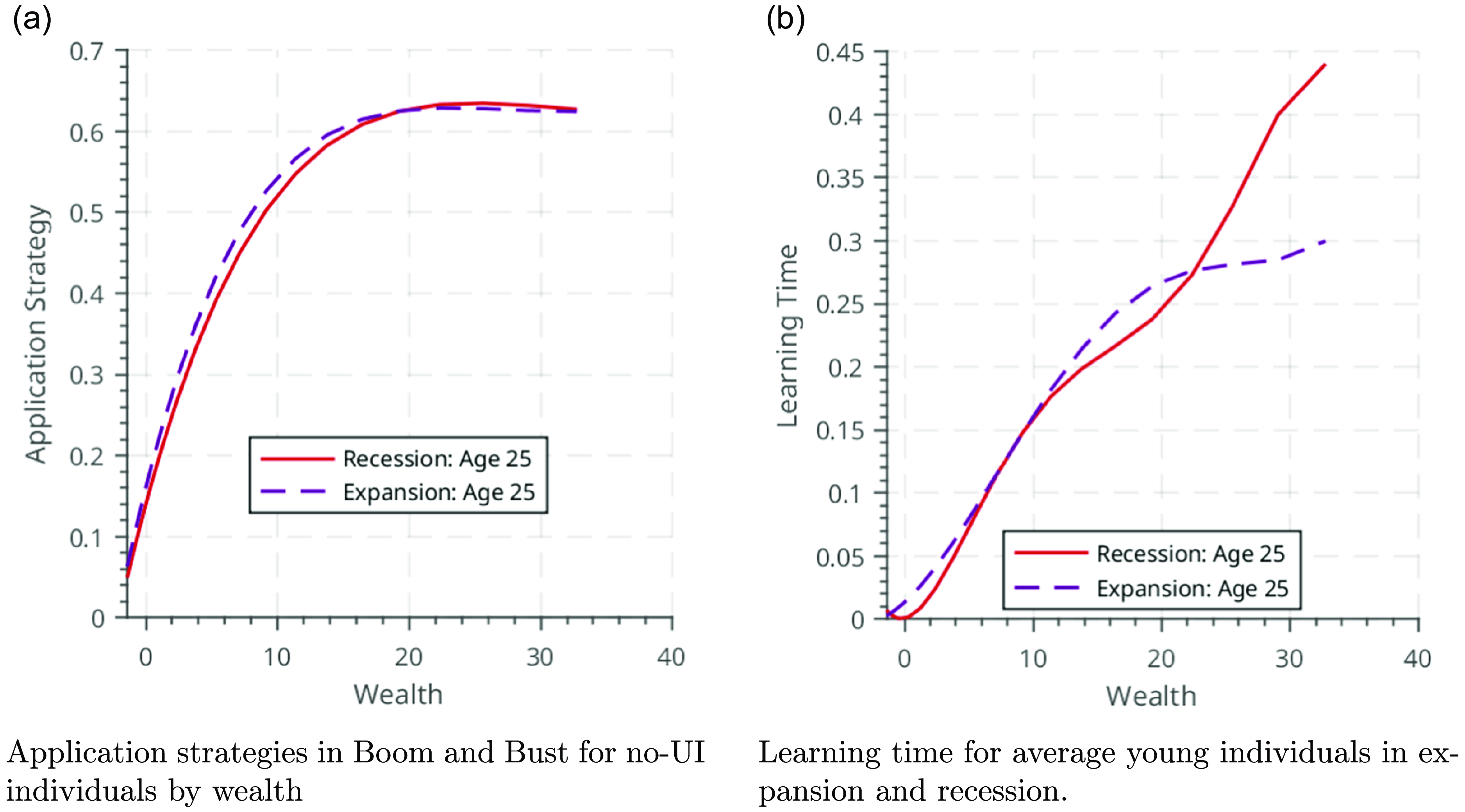
Figure 6. Decision rules by different dimensions of heterogeneity.
4.3 Impact of wealth inequality on recessions
To illustrate the importance of wealth heterogeneity in driving the aggregate response to a recession, we conduct counterfactual experiments in which we subject the economy to the same aggregate shock as above, but either increase or decrease wealth dispersion immediately prior to entering an identical-sized recession. Both counterfactuals take the form of a mean-preserving change in the wealth distribution.
Figure 7 reports the results; “spread decrease” and “spread increase” refer to a 10% narrower and 10% wider time- $0$
wealth distribution, respectively. The exercises illustrate that a wider time-
$0$
wealth distribution, respectively. The exercises illustrate that a wider time- $0$
wealth distribution amplifies the effect of a productivity shock on economic aggregates, in particular average human capital. Notably, the effect on average human capital manifests itself largely over the longer horizon rather than on impact. Lower wealth of the wealth-poor amplifies the reduction in their human capital accumulation, but this does not instantly produce large earnings losses as it takes time for these individuals to become a significant fraction of the employed human capital stock.
$0$
wealth distribution amplifies the effect of a productivity shock on economic aggregates, in particular average human capital. Notably, the effect on average human capital manifests itself largely over the longer horizon rather than on impact. Lower wealth of the wealth-poor amplifies the reduction in their human capital accumulation, but this does not instantly produce large earnings losses as it takes time for these individuals to become a significant fraction of the employed human capital stock.
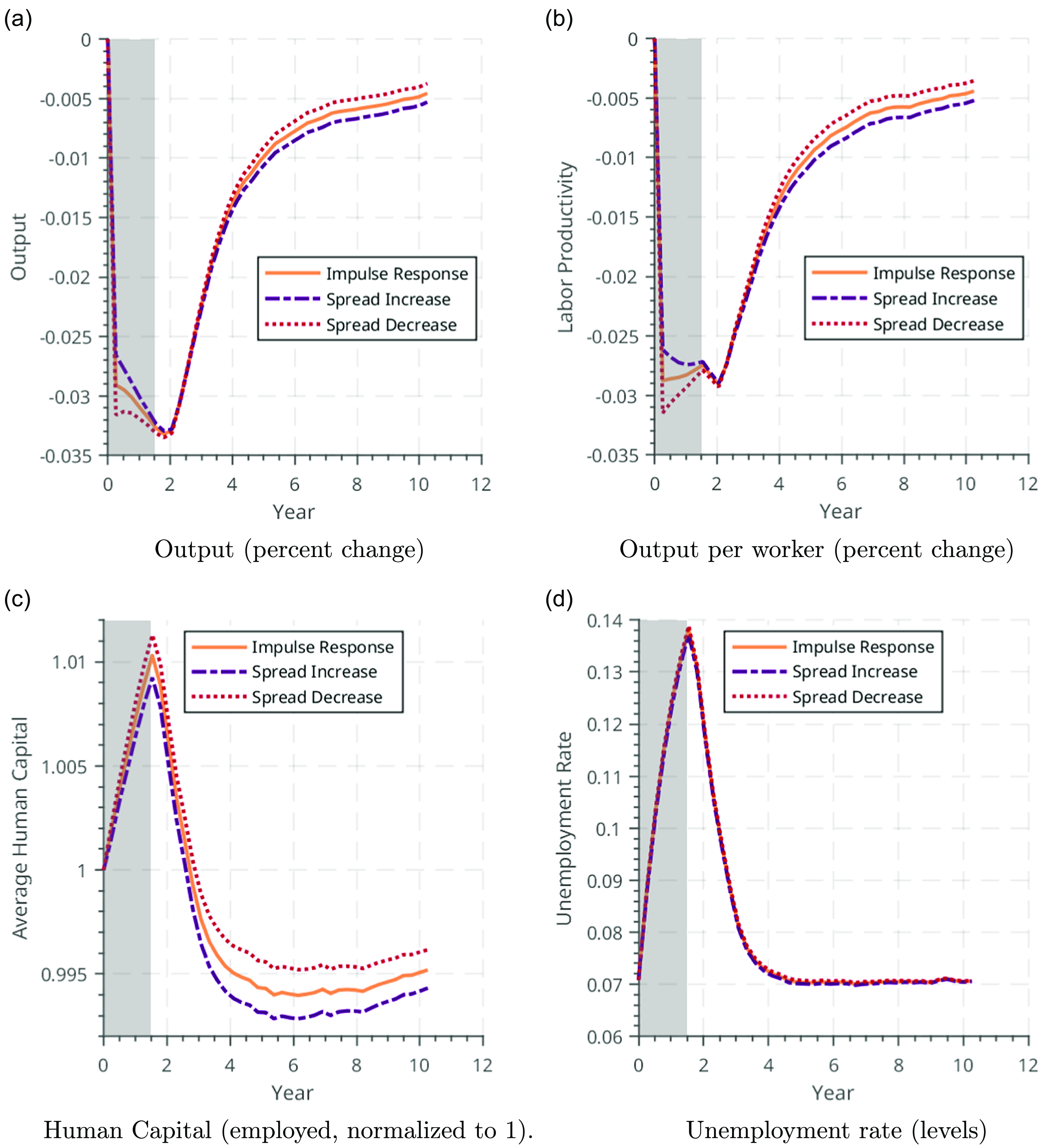
Figure 7. Effects of a negative productivity shock, various initial wealth distributions.
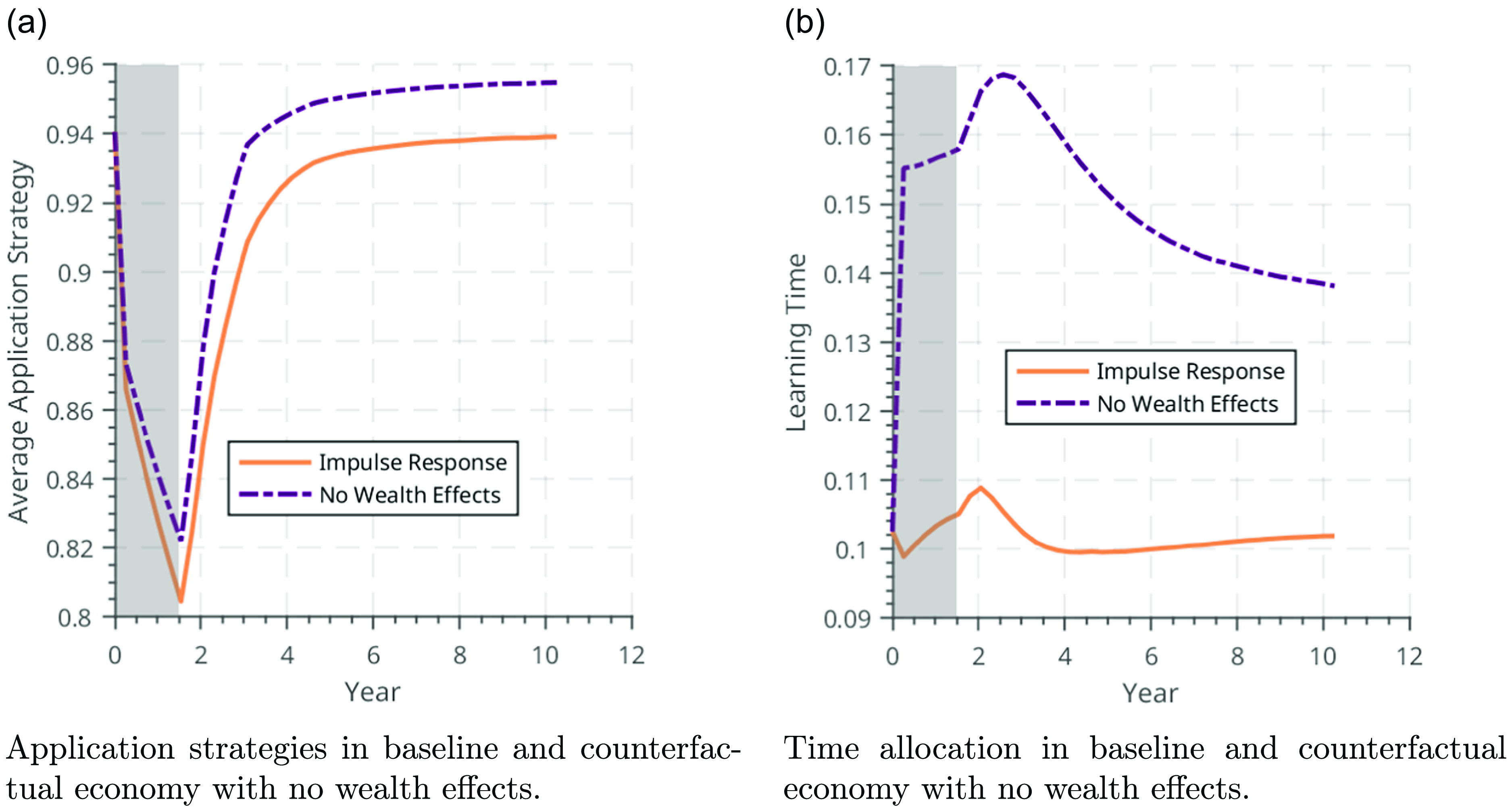
Figure 8. Impact of wealth effects on decision rules.
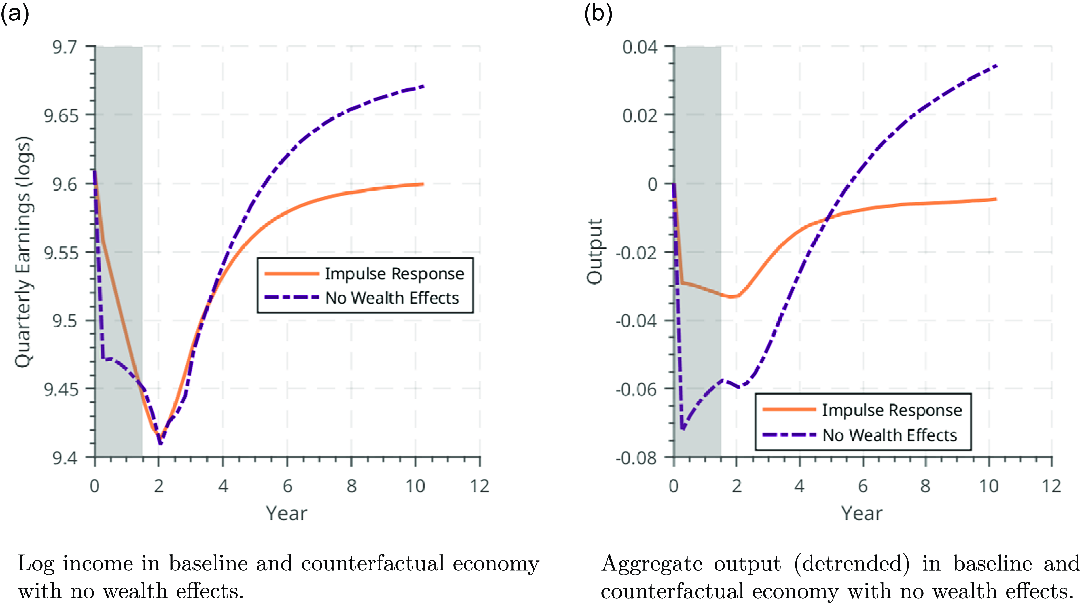
Figure 9. Impact of wealth effects on downturn and recovery.
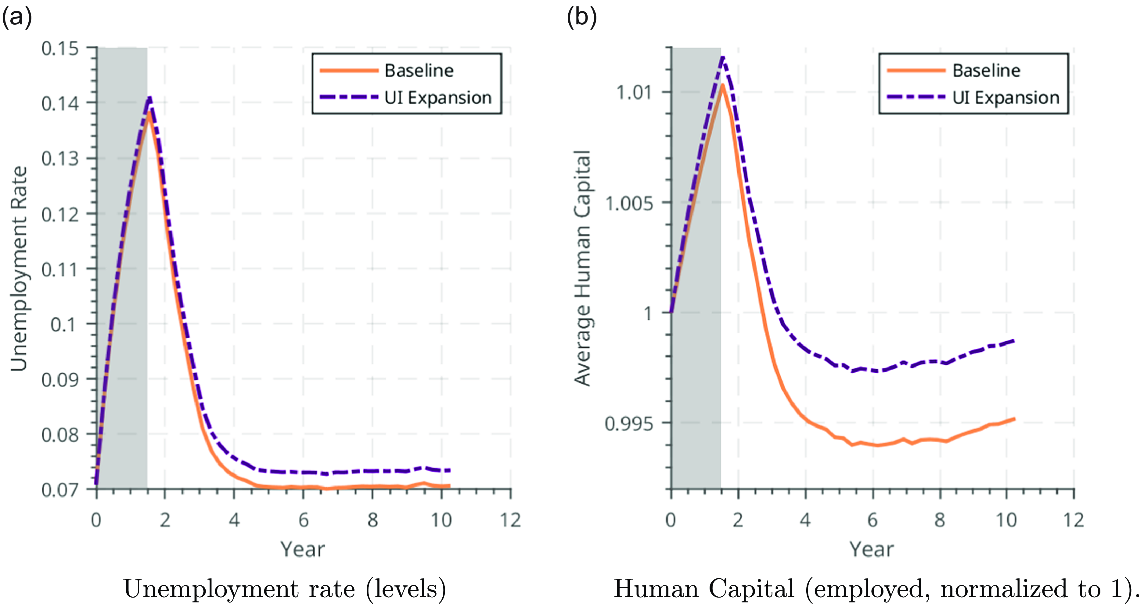
Figure 10. Effects of a negative productivity shock, increase in expected UI duration.
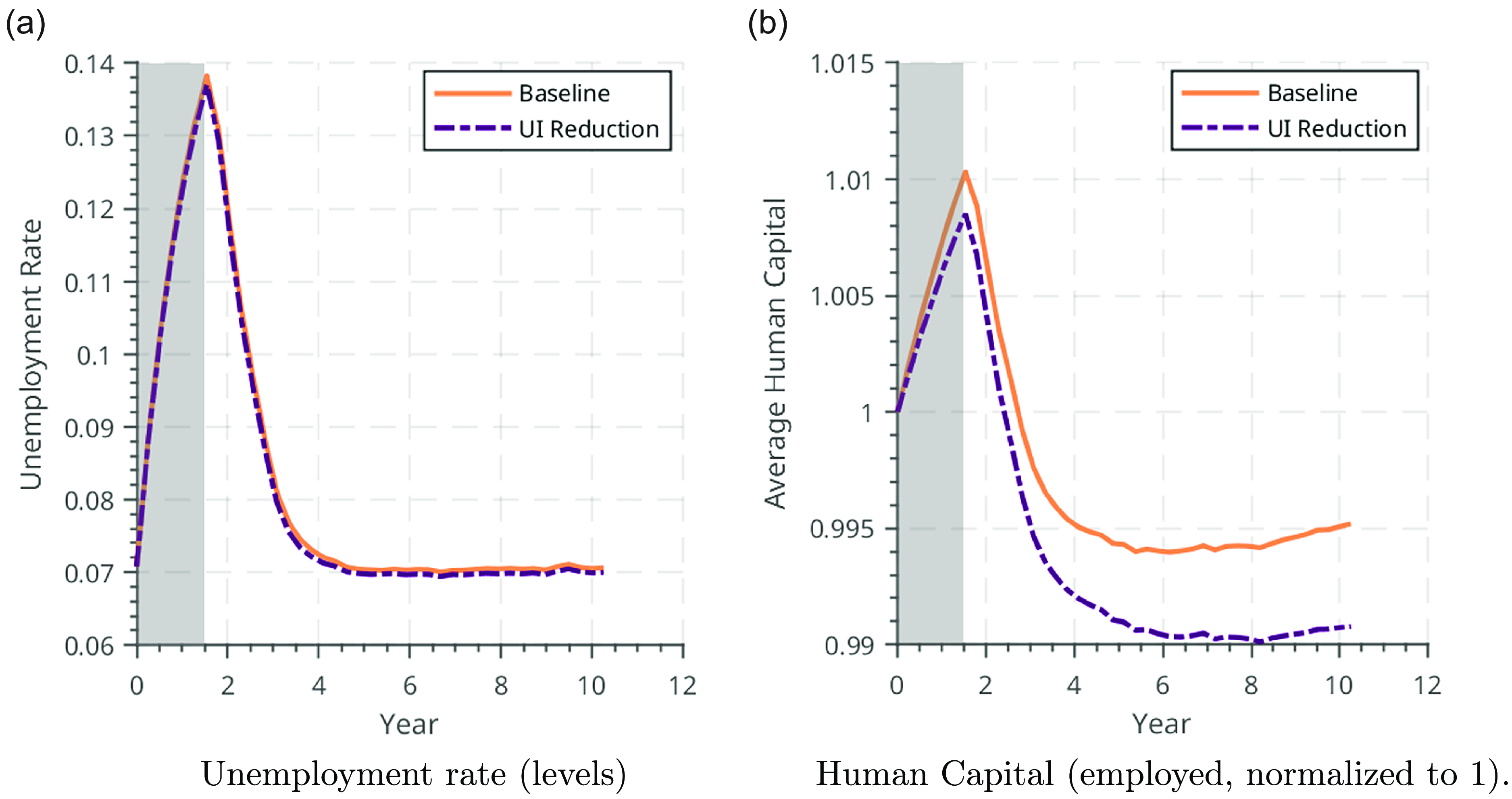
Figure 11. Effects of a negative productivity shock, decrease in expected UI duration.
Last, we conduct a decomposition exercise in which we eliminate the presence of wealth effects entirely. In this experiment, all agents behave as though they have the average steady-state level of wealth across the baseline simulation, but retain their other dimensions of initial heterogeneity. We plot the impact on application strategy (left panel) and time allocation (right panel) in Figure 8.
While the impact on application strategies is present, the change in time allocation is sizable: absent wealth effects, agents allocate a 33% more of their available time to building human capital during recessions. The resulting impact on the economy is tangible: the absence of wealth effects changes both the depth of the recession, and the size and speed of recovery. In Figure 9, we plot log income and aggregate output (detrended) for the baseline economy (gold, solid line) and counterfactual economy without wealth effects (purple, dash-dotted line), in the left and right panels, respectively.
On impact, employment falls more in the economy without wealth effects; output falls more on impact in the economy without wealth effects, but then exhibits a faster and stronger recovery. This results from two forces. First, without wealth effects, workers apply for higher pay, more difficult to obtain jobs, as shown in Figure 8a. Second, and more importantly, they allocate more time to human capital accumulation, which results in a larger initial drop in output (due to reallocation of time toward learning) but also in a larger and more rapid economic recovery, and therefore a smaller cumulative output drop. We quantify these differences between the economy with no wealth effects and the benchmark in Table 7.
Eliminating wealth effects leads to an increase in output and earnings of 0.2% and 0.25%, respectively. This occurs because human capital grows by 4.27% as a result of workers reallocating their time towards learning. Perhaps more notably, earnings and output increase despite a 39% increase in time allocated to human capital accumulation. Despite the resulting reduction in hours available for work, this counterfactual economy is more productive, showing the magnitude and importance of the wealth effects present in our model.
The above results highlight the interaction of wealth with human capital accumulation as the key propagation mechanism. This raises the question of what role search frictions play. While indirect, the effect of search frictions is crucial. Compared to a model with competitive labor markets, directed search generates endogenous dependence of future wages on wealth. Wealth-poor unemployed workers apply for jobs that pay less, but are easier to obtain. This means that low wealth when unemployed leads to persistent earnings losses. Anticipating this effect when employed, workers have an additional precautionary motive to accumulate savings—and therefore forego human capital accumulation—that would be absent in a model with competitive labor markets such as Huggett et al. (Reference Huggett, Ventura and Yaron2011). Indeed, as shown by Griffy (Reference Griffy2021), while the interaction between wealth and human capital is key, wealth affects human capital accumulation much more in a model with search frictions than without them.
4.4 Policy experiments: unemployment insurance
Table 8. Estimated auxiliary parameters from elasticity and age-regression moments
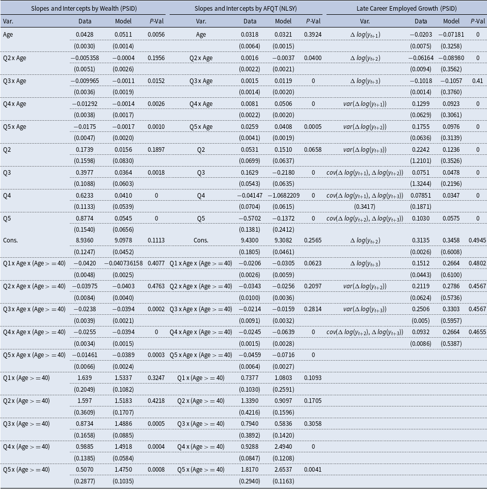
Table 9. Estimated auxiliary parameters from job-to-job transition rate by wealth
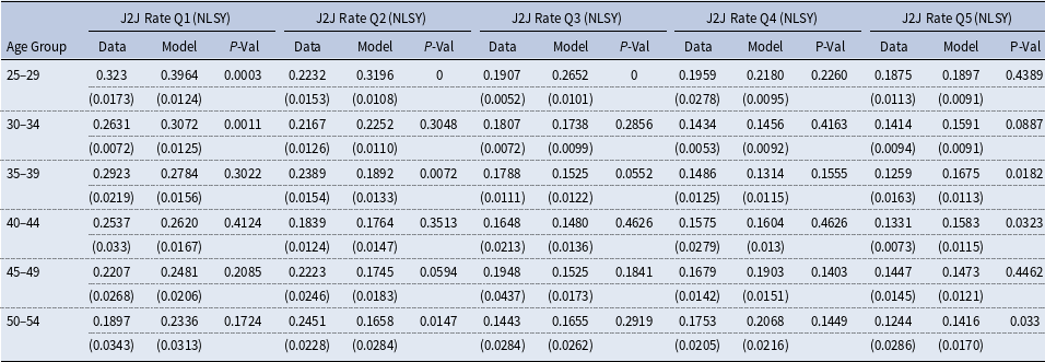
Table 10. Estimated auxiliary parameters from job-to-job earnings growth by wealth
This intuition suggests that policies insuring workers against unemployment risk will also impact human capital accumulation. We confirm this through policy experiments in which we vary the duration of unemployment insurance, $\gamma$
. The counterfactual experiments below, shown in Figure 10 and Figure 11, entail an increase or decrease in UI duration, respectively, contemporaneously with the negative productivity shock. Consistent with the mechanism described above, a UI increase dampens the decline in human capital in response to the negative productivity shock.
$\gamma$
. The counterfactual experiments below, shown in Figure 10 and Figure 11, entail an increase or decrease in UI duration, respectively, contemporaneously with the negative productivity shock. Consistent with the mechanism described above, a UI increase dampens the decline in human capital in response to the negative productivity shock.
5. Conclusion
Our analysis takes a step toward understanding how an economy’s wealth distribution shapes its labor market and productivity dynamics. The specific channel explored here has to do with heterogeneous responses of on-the-job training by wealth. We show that our heterogeneous-agent model implies a substantial drop in human capital in response to a recession, and that this drop in human capital would be dampened under a less dispersed wealth distribution.
Table 11. Comparison with Davis von Wachter (2011)
Our findings have important policy implications. Even in the absence of aggregate uncertainty, the framework used here implies that redistributive policies such as progressive taxation or unemployment insurance have the potential to not only provide insurance but also increase aggregate earnings and human capital. They can do so by changing both the job search strategies of the unemployed and the on-the-job training decisions of the employed. With aggregate shocks, our findings suggest that such policies may also serve to dampen the aggregate response to an aggregate downturn.
Our focus has been on the effects of the wealth distribution on economic aggregates. Methodologically, our framework also naturally lends itself to a related but distinct question: the heterogeneous effects of a recession by wealth. In particular, there is a well established set of important results empirically documenting persistent earnings costs of job displacement (Jacobson et al. (Reference Jacobson, LaLonde and Sullivan1993), Davis and von Wachter (Reference Davis and von Wachter2011)) and persistent earnings costs of entering the labor market in a recession (Kahn (Reference Kahn2010)), which has also spawned a substantial theoretical literature incorporating these channels into labor market search models (see e.g. Guo (Reference Guo2018), Wee (Reference Wee2013), Huckfeldt (Reference Huckfeldt2022), and Acabbi et al. (Reference Acabbi, Alati and Mazzone2023)). This literature has abstracted, however, from the effects of wealth on labor market decisions, often assuming risk neutral agents. Our analysis suggests that such scarring effects may differ systematically by wealth through its effect on both job search and human capital. A full examination of such heterogeneous effects is an important agenda for future research.
Acknowledgements
We would like to thank the editor as well as two anonymous referees for their helpful comments and feedback. We also thank seminar and conference participants at the University at Albany, SUNY, Saint Lawrence University, the University of Rochester, the University of Helsinki, the University of Bristol, the European Winter Meetings of the Econometric Society (2019), the Southern Economic Association meetings in Houston (2019), the Midwest Macroeconomics Fall Meeting (2019), the Econometric Society World Congress (2020), the Spanish Economic Association meetings in Barcelona (2021).


 Open access