

1. Introduction
Many (perhaps most) papers in top conferences these days propose methods and test them on standard benchmarks such as General Language Understanding Evaluation (GLUE)Footnote a (Wang et al. Reference Wang, Singh, Michael, Hill, Levy and Bowman2018), Multilingual Unsupervised and Supervised Embeddings (MUSE)Footnote b (Conneau et al. Reference Conneau, Lample, Ranzato, Denoyer and Jégou2017), and wordnet 18 reduced relations (WN18RR) (Dettmers et al. Reference Dettmers, Minervini, Stenetorp and Riedel2018). Some of these methods (Bidirectional Encoder Representations from Transformers (BERT) Devlin et al. Reference Devlin, Chang, Lee and Toutanova2019, enhanced representation through knowledge integration (ERINE) Sun et al. Reference Sun, Wang, Li, Feng, Tian, Wu and Wang2020) not only do well on benchmarks but also do well on tasks that we care about.Footnote c Unfortunately, despite large numbers of papers with promising performance on benchmarks, there is remarkably little evidence of generalizations beyond benchmarks.
In my last Emerging Trends column (Church Reference Church2020), I complained about reviewing. Reviewers do what reviewers do. They love papers that are easy to review. Reviewers give high grades to boring incremental papers that do slightly better than SOTA (state of the art) on an established benchmark. No one ever questions whether the benchmark is still relevant (or whether it was ever relevant). Generalizing beyond the benchmark is of little concern. Precedent is good (and simple to review). Impact is too much work for the reviewers to think about.
Benchmarks have a way of taking on a life of their own. Benchmarks tend to evolve over time. When the benchmark is first proposed, there is often a plausible connection between the benchmark and a reasonable goal that is larger than the benchmark. But this history is quickly forgotten as attention moves to SOTA numbers, and away from sensible (credible and worthwhile) motivations.
2. The goal
Before discussing some of the history behind MUSE and WN18RR, benchmarks for bilingual lexicon induction (BLI) and knowledge graph completion (KGC), it is useful to say a few words about goals. It is important to remember where we have been, but even more important to be clear about where we want to go.
I do not normally have much patience for management books, but “The Goal” (Goldratt 1984) is an exception.Footnote d The point is that one should focus on what matters and avoid misleading internal metrics. Goldratt invents a fictional factory to make his point. The fictional factory is losing money because of misleading internal metrics. They should be focused on end-to-end profit, a combination of three factors: (1) throughput (sales), (2) inventory costs, and (3) operational expense. But in the story, they introduced a misleading metric (output per hour), which appeared to be moving in the right direction when they introduced automation (robots), but in fact, the robots were increasing cost, because most of the output was ending up in inventory. The moral of the story is that we need to focus on what matters (end-to-end results). It can be helpful to factor a complicated system into simpler units that are easier to work with (unit testing is often easier and more actionable than system testing), but we need to make sure the simplification is on the critical path toward the goal.
Another exampleFootnote e is a jewelry business. Unlike the fictional factory, this is a real example. This jewelry business has lots of products (and consequently, lots of inventory). Products have a long tail. Some products sell faster than others. The right metrics helped the business focus on key bottlenecks. Two simple process improvements increased sales:
1. The business had been prioritizing too many products, but better metrics encouraged them to prioritize products by sales. Make sure that shelves are stocked with fast movers, before stocking shelves with other products.
2. In addition, if a product has been in a store for a while and has not sold, rotate it to another store. Some products sell better in some markets and other products sell better in other markets.
The moral, again, is to focus on the right metrics. Without focus, there is a tendency to optimize everything. But most systems are constrained by a few bottlenecks. Optimize bottlenecks (and nothing else). Misleading metrics are worse than useless because of opportunity costs. The wrong metrics distract attention from what matters (addressing bottlenecks) and encourage wasted effort optimizing steps that are not on the critical path toward the goal. Resist the temptation to optimize everything (because most things are not on the critical path toward the goal).
What does this have to do with benchmarks? Benchmarks can be a useful step toward the goal (when the benchmark is on the critical path), as demonstrated by the GLUE benchmark, and deep nets such as BERT and ERNIE. The case for other benchmarks such as MUSE and WN18RR is less well established. Survey articles (Nguyen Reference Nguyen2017) mention many KGC algorithms: Trans[DEHRM], KG2E, ConvE, Complex, DistMult, and more (Bordes et al. Reference Bordes, Usunier, Garcia-Duran, Weston and Yakhnenko2013; Wang et al. Reference Wang, Zhang, Feng and Chen2014; Yang et al. 2015; Lin et al. Reference Lin, Liu, Sun, Liu and Zhu2015; Trouillon et al. Reference Trouillon, Welbl, Riedel, Gaussier and Bouchard2016; Nguyen et al. Reference Nguyen2017; Nickel, Rosasco, and Poggio Reference Nickel, Rosasco and Poggio2019; Sun et al. Reference Sun, Deng, Nie and Tang2019). Many of these perform well on the benchmark, but it remains to be seen how this work improves coverage of WordNet (Miller Reference Miller1998). Will optimizing P@10 on WN18RR produce more complete knowledge graphs? Has WordNet coverage improved as a result of all this work on the KGC WN18RR benchmark? If not, why not? When should we expect to see such results?
3. Background: Rotation matrices, BLI and KGC
Rotation matrices play an important role in both BLI and KGC. Benchmarks in both cases provide various resources (embeddings Mikolov, Le, and Sutskever Reference Mikolov, Le and Sutskever2013; Pennington, Socher, and Manning Reference Pennington, Socher and Manning2014; Mikolov et al. Reference Mikolov, Grave, Bojanowski, Puhrsch and Joulin2017) as well as test and train sets. In particular, MUSEFootnote f provides embeddings in 45 languages, as well as training and test dictionaries (in both directions) between English (en) and 44 other languages: af, ar, bg, bn, bs, ca, cs, da, de, el, es, et, fa, fi, fr, he, hi, hr, hu, id, it, ja, ko, lt, lv, mk, ms, nl, no, pl, pt, ro, ru, sk, sl, sq, sv, ta, th, tl, tr, uk, vi, zh. In addition, MUSE provides bilingual dictionaries for all pairs of six languages: en, de, es, fr, it, pt. (This paper will use ISO 639-1 for languages).Footnote g
The training dictionaries are also known as seed dictionaries. Seed dictionaries, S, consist of  $|S|$ pairs of translation equivalents, $<x_i , y_j >$
, where
$<x_i , y_j >$
, where  $x_i$
is a word in source language x and
$x_i$
is a word in source language x and  $y_j$
is a word in target language y. These dictionaries are used to train a rotation. That is, we construct two arrays, X and Y, both with dimensions
$y_j$
is a word in target language y. These dictionaries are used to train a rotation. That is, we construct two arrays, X and Y, both with dimensions  $|S| \times K$
. Rows of X are
$|S| \times K$
. Rows of X are  $vec(E_x , x_i)$
and rows of Y are
$vec(E_x , x_i)$
and rows of Y are  $vec(E_y , y_i)$
, where
$vec(E_y , y_i)$
, where  $vec(E_x,x_i)$
looks up the word
$vec(E_x,x_i)$
looks up the word  $x_i$
in the embedding,
$x_i$
in the embedding,  $E_x$
for language x. Embeddings,
$E_x$
for language x. Embeddings,  $E_x$
and
$E_x$
and  $E_y$
have dimensions,
$E_y$
have dimensions,  $V_x \times K$
and
$V_x \times K$
and  $V_y \times K$
, respectively, where
$V_y \times K$
, respectively, where  $V_x$
and
$V_x$
and  $V_y$
are the sizes of the vocabularies for the two languages.
$V_y$
are the sizes of the vocabularies for the two languages.
The training process solves the objective:
 \begin{equation} \min_{R_{x,y}} \|X R_{x,y} - Y\|_F^2 \ \ \ \text{where} \ \ \ R_{x,y} \in \mathcal{R}^{K\times K}\end{equation} $R_{x,y}$
is a
$R_{x,y}$
is a  $K \times K$
rotation matrix that translates vectors in language x to vectors in language y. A simple solution for R is the Orthogonal Procrustes problem.Footnote h
$K \times K$
rotation matrix that translates vectors in language x to vectors in language y. A simple solution for R is the Orthogonal Procrustes problem.Footnote h
At inference time, we are given a new source word,  $x_i$
in the source language x. The task is to infer
$x_i$
in the source language x. The task is to infer  $trans_{x,y} (x_i) = y_j$
, where
$trans_{x,y} (x_i) = y_j$
, where  $y_i$
is the appropriate translation in target language y. The standard method is to use Equation (2), where
$y_i$
is the appropriate translation in target language y. The standard method is to use Equation (2), where  $vec^{-1}$
is the inverse of vec. That is,
$vec^{-1}$
is the inverse of vec. That is,  $vec^{-1}$
looks up a vector in an embedding and returns the closest word.
$vec^{-1}$
looks up a vector in an embedding and returns the closest word.
 \begin{equation} trans_{x,y} (x_i) \approx vec^{-1}( E_y, \, vec(E_x,x_i) \, R_{x,y} )\end{equation}
Much of the BLI literature improves on this method by taking advantage of constraints such as hubness (Smith et al. Reference Smith, Turban, Hamblin and Hammerla2017). Most words have relatively few translations, and therefore, the system should learn a bilingual lexicon with relatively small fan-in and fan-out. Hubs are undesirable; we do not want one word in one language to translate to too many words in the other language (and vice versa).
Consider random walks over MUSE dictionaries. If we start with bank in English, we can translate that to banco and banca in Spanish. From there, we can get back to bank in English, as well as bench.
 \begin{equation} bank \rightarrow banco|banca \rightarrow bank|bench\end{equation}
Table 1 shows that most words (in the MUSE challenge) have very limited fan-out. In fact, most words are disconnected islands, meaning they back-translate to themselves and nothing else (via random walks over 45 language pairs).
Fan-out for 168k English words in MUSE, most of which (115k) are disconnected islands that back-translate to themselves (and nothing else). The majority of the rest back-translate to five or more words

Taking advantage of hubness clearly improves performance on the MUSE challenge, but why? Hopefully, the explanation is the one above (most words have relatively few translations), but it is also possible that hubness is taking advantage of flaws in the benchmark such as gaps in MUSE (most words should have many more translations than those in MUSE (Kementchedjhieva, Hartmann, and Søgaard Reference Kementchedjhieva, Hartmann and Søgaard2019)).
3.1 Knowledge Graph Completion (KGC)
KGC benchmarks (WN18RR) are similar to BLI mechmarks (MUSE). Many of these KGC algorithms (and evaluation sets) are now available in pykg2vec (Yu et al. Reference Yu, Rokka Chhetri, Canedo, Goyal and Faruque2019), a convenient Python package.Footnote i The goal of KCG, presumably, is to improve coverage of knowledge graphs such as WordNet.
KGC starts with  $<h,r,t>$
triples, where h (head) and t (tail) are entities (words, lemmas, or synsets) connected by a relation r. For example, the antonymy relationship
$<h,r,t>$
triples, where h (head) and t (tail) are entities (words, lemmas, or synsets) connected by a relation r. For example, the antonymy relationship  $<$
inexperienced,
$<$
inexperienced,  $\ne$
, experienced
$\ne$
, experienced  $>$
, is a triple where h is inexperienced, r is
$>$
, is a triple where h is inexperienced, r is  $\neq$
and t is experienced. Heads and tails are typically represented as vectors, and relations are represented as rotation matrices. Thus, for example, antonymy could be modeled as a regression task: vec(inexperienced
$\neq$
and t is experienced. Heads and tails are typically represented as vectors, and relations are represented as rotation matrices. Thus, for example, antonymy could be modeled as a regression task: vec(inexperienced  $) \sim vec$
(experienced), where the slope of this regression is a rotation matrix. In this case, the rotation matrix is an approximation of the meaning of negation.
$) \sim vec$
(experienced), where the slope of this regression is a rotation matrix. In this case, the rotation matrix is an approximation of the meaning of negation.
Benchmarks such as WN18RR are incomplete subsets of WordNet. WN18RR consists of 41k entities (WordNet synsets) and 11 relations, though just 2 of the relations cover most of the test set. We can model triples as graphs,  $G_{r} = (V,E)$
, one for each relation r, where V is a set of vertices (h and t), and E is a set of edges connecting h to t. WN18RR splits edges, E, into train, validation and test randomly, with 60% in train, and 20% in each of the other two sets. At training time, we learn a model from the training set. At inference time, we apply that model to a query from the test set,
$G_{r} = (V,E)$
, one for each relation r, where V is a set of vertices (h and t), and E is a set of edges connecting h to t. WN18RR splits edges, E, into train, validation and test randomly, with 60% in train, and 20% in each of the other two sets. At training time, we learn a model from the training set. At inference time, we apply that model to a query from the test set,  $\lt h,r,? \gt $
or
$\lt h,r,? \gt $
or  $<?,r,t>$
. The task is to fill in the missing value. N-best candidates are scored by precision at ten (P@10).
$<?,r,t>$
. The task is to fill in the missing value. N-best candidates are scored by precision at ten (P@10).
This setup is more meaningful when edges are iid, though WordNet makes considerable use of equivalence relations (synonyms), apartness relations (antonyms), partial orders (is-a, part-of), and other structures that are far from iid.
Unstructured: Edges are iid. If we tell you there is (or is not) an edge between h and t, we have provided no information about the rest of the graph.
Structured: Edges are not iid. Examples: equivalence classes and partial orders.
WN18RR is an improvement over an earlier benchmark, WN18, which suffered from information leakage (Dettmers et al. Reference Dettmers, Minervini, Stenetorp and Riedel2018). WordNet documentationFootnote j makes it clear that various links come in pairs (by construction). If a car is a vehicle, for example, then there will be both a hypernym link in one direction, as well as a hyponym link in the other direction. Similar comments apply to other relations such as part-of. WN18 originally had 18 relations, but the 18 were reduced down to 11 in WN18RR.
WN18RR addresses some of the leakage, but there is more. Most of the test set is dominated by 2 of the 11 relations, hyperym and derivationally related forms. The former is a partial order (is-a) and the latter is (nearly) an equivalence relation, combining aspects of morphology with synonymy. We recently submitted a paper questioning the use of iid assumptions for equivalence relations. It turns out that one can do very well on the benchmark (without addressing the goal of improving WordNet coverage) because much of the test set can be inferred from random walks (and transitivity) from triples in the training set.
4. WordNet is incomplete because it is too English-centric
The missing at random model does not pay enough respect to Miller, an impressive researcher (and Chomsky’s mentor). One is unlikely to improve his work much by the kinds of methods that have been discussed thus far such as rotation matrices and random walks. To make meaningful progress, we need to bring something to the table (such as more languages) that goes well beyond the topics that Miller was thinking about.
Miller was focused on English. WordNets are now available in German (Hamp and Helmut Reference Hamp and Feldweg1997), Chinese (Dong, Dong, and Hao Reference Dong, Dong and Hao2010), and many other languages.Footnote k The Natural Language Toolkit (NLTK) interface to WordNetFootnote l supports 29 languages: ar, bg, ca, da, el, en, es, eu, fa, fi, fr, gl, he, hr, id, it, jp, ms, nb, nl, nn, pl, pt, qc, sl, sq, sv, th, zh.Footnote m Coverage varies considerably by language. Few languages have as much coverage as English. Some have considerably less.
Table 2 illustrates glosses in English (en) and French (fr) for five synsets of bank. All five synsets have a single gloss in English. Two synsets have two glosses in French, and one has none.
Five synsets in two (of 29) languages

The basic framework was developed for English. As WordNet becomes more and more multilingual, it needs to move away from viewing English as a pivot language toward a more language universal inter-lingua view of world knowledge. Ultimately, the knowledge completion goal should aim higher than merely capturing what is already in WordNet (English-centric knowledge) to something larger (world knowledge). Benchmarks such as WN18RR distract us away from the larger goal (capturing world knowledge that goes beyond the English-centric view that Miller was working with), to something smaller than what Miller was thinking about (how to capture subsets of English from other subsets of English).
Other languages bring new insights to the table. We recently submitted a paper proposing a new similarity metric, backsim (back-translation similarity). Backsim uses bilingual dictionaries in MUSE to find 316k pairs of words like similarly and likewise that have similar translations in other languages. We suggested that many (271k) of these pairs should be added to WordNet under four relations: M (morph), S (synonym), H (hypernym), and D (derived form). In this way, other languages help us move from our own view of our language toward world knowledge.
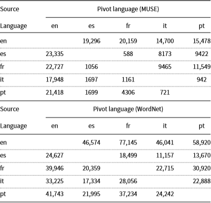
Vocabulary Sizes (excluding disconnected islands). Numbers are larger for WordNet than MUSE, suggesting WordNet has better coverage. Numbers are also larger for English (en) than other languages, suggesting both WordNet and MUSE have better coverage of English than other languages
4.1 Comparisons of WordNet and MUSE
We have an embarrassment of riches now that WordNet is available in 29 languages, and MUSE is available in 45 languages. Comparisons of the two (Tables 3–5) suggest WordNet has remarkably good coverage, probably better than MUSE. Researchers in BLI would be well advised to consider WordNet in addition to (or perhaps as a substitute for) the bilingual dictionaries in MUSE.
Table 3 compares MUSE and WordNet vocabulary sizes after removing disconnected islands. Let  $M_{x,y}$
be a sparse matrix with a non-zero value in cell i, j if there is a translation from
$M_{x,y}$
be a sparse matrix with a non-zero value in cell i, j if there is a translation from  $x_i$
to
$x_i$
to  $y_j$
, where
$y_j$
, where  $x_i$
is a word in language x and
$x_i$
is a word in language x and  $y_j$
is a word in language y. We then form
$y_j$
is a word in language y. We then form  $M_{x,x} = M_{x,y} M_{y,x}$
. This matrix,
$M_{x,x} = M_{x,y} M_{y,x}$
. This matrix,  $M_{x,x}$
, tells us how words in language x can back-translate via the pivot language y. Most words back-translate to themselves and nothing else. We refer to these words as disconnected islands. We are more interested in words with more translation possibilities.
$M_{x,x}$
, tells us how words in language x can back-translate via the pivot language y. Most words back-translate to themselves and nothing else. We refer to these words as disconnected islands. We are more interested in words with more translation possibilities.
Table 3 suggests WordNet has better coverage than MUSE since numbers are larger for WordNet than MUSE. In addition, the table suggests that both WordNet and and MUSE have better coverage of English (en) than other languages.
Some of the numbers in Table 3 are embarrassingly small, especially for MUSE. Numbers under 10k are suspiciously low. In MUSE, some languages have only 1k words with more than one back translation ( $\approx 1\%$
of the total vocabulary). In other words, some of the MUSE dictionaries are close to a substitution cipher. This may explain why hubness has been so effective for MUSE. But if this is the explanation, it may cast doubt on how effective hubness methods will be for generalizing beyond the benchmark.
$\approx 1\%$
of the total vocabulary). In other words, some of the MUSE dictionaries are close to a substitution cipher. This may explain why hubness has been so effective for MUSE. But if this is the explanation, it may cast doubt on how effective hubness methods will be for generalizing beyond the benchmark.
WordNet (WN) has more French glosses than MUSE

WordNet has more French glosses than MUSE. Each cell, i, j, counts the number of words with i glosses in WordNet and j glosses in MUSE
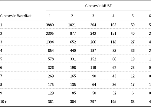
Tables 4–5. dive deeper into French glosses. These tables show the number of glosses for nearly 18k English words that have at least 1 gloss in both collections. Of these, there are 10,330 words with more French glosses in WordNet, and 2266 with more in MUSE, and 5125 with the same number of French glosses in both collections.
In addition to simple counts, we would like to know if we are covering the relevant distinctions. One motivation for word senses is translation. Bar-Hillel (Reference Bar-Hillel1960) left the field of machine translation because he could not see how to make progress on word sense disambiguation (WSD). The availability of parallel corpora in the early 1990s created an opportunity to make progress on Bar-Hillel’s concerns. WSD could be treated as a supervised machine learning problem because of an interaction of word senses and glosses, as illustrated in Table 6 (Gale, Church, and Yarosky Reference Gale, Church and Yarosky1992).
Interaction between word sense (English) and glosses (French)

How effective are WordNet and MUSE on examples such as those in Table 6? Unfortunately, WordNet glosses both bank.n.01 and bank.n.06 with banque, even though the definitions and examples make it clear that bank.n.01 is a river bank, and bank.n.06 is a money bank. Similarly, WordNet glosses for drug mention drogue but not médicament, possibly because this legal/illegal distinction is less salient in English. It is well known in lexicography that monolingual concerns are different from bilingual concerns. One should not expect a taxonomy of English synsets to generalize very well to all the worlds’ languages. Thus, we see gaps across languages as a better opportunity to improve WordNet than gaps within English. Miller already thought quite a bit about coverage within English, but not so much about coverage across languages.
In short, spot checks are not encouraging; the coverage of glosses in WordNet and MUSE are probably inadequate for WSD applications, at least in the short term, where other approaches to WSD are more promising. Longer term, we see WSD applications, especially in a bilingual context, as an opportunity to test KGC, with less risk of leakage than benchmarks such as WN18RR. That is, the task is not to predict held-out edges but to predict translations of polysemous words into other languages. There is no shortage of testing and training material for this task, given how much text is translated, and how many of those words are polysemous. For a task like this, one might expect methods based on Machine Translation (Wu et al. Reference Wu, Schuster, Chen, Le, Norouzi, Macherey, Krikun, Cao, Gao, Macherey, Klingner, Shah, Johnson, Liu, Kaiser, Gouws, Kato, Kudo, Kazawa, Stevens, Kurian, Patil, Wang, Young, Smith, Riesa, Rudnick, Vinyals, Corrado, Hughes and Dean2016) and/or BERT/ERNIE Transformers (Devlin et al. Reference Devlin, Chang, Lee and Toutanova2019; Sun et al. Reference Sun, Wang, Li, Feng, Tian, Wu and Wang2020) to offer stronger baselines than traditional KGC methods.
4.2 WordNet as a database: Unifying BLI and KGC
Thus far, we have been treating bilingual lexicons and knowledge representation as separate problems, but there are aspects of both in WordNet, which become more salient when we view WordNet as a simple database. The proposed database view factors some facts into tables that depend on language, and other facts into tables that are language universal.
This database view of WordNet combines various aspects of both MUSE and WN18RR. WordNet has glosses over multiple languages (like MUSE), as well as relations over entities (like WN18RR). The schema is a bit more complicated than both MUSE and WN18RR because there are multiple tables (some depend on language and some do not), and three types of entities: synsets, lemmas, and strings (glosses, examples, and definitions).
1. Synset relations: $< h, r, t>$
where h (head) and t (tail) are synsets and r is a member of a short list of relations on synsets (e.g., is-a, part-of).
$< h, r, t>$
where h (head) and t (tail) are synsets and r is a member of a short list of relations on synsets (e.g., is-a, part-of).2. Definitions: maps 118k synsets to definitions (English strings).
3. Examples: maps 33k (of 118k) synsets to examples (English strings).
4. Synset2lemmas: maps synset to 0 or more lemmas in 29 languages
5. Lemma Glosses: maps lemma objects to glosses (strings) in 29 languages
6. Lemma Relations:
$< h, r, t, lang>$
, where h and t are lemmas and r is a member of a short list of relations on lemmas (e.g., derivationally related forms, synonyms, antonyms, and pertainyms), and lang is one of 29 languages.


Sizes of these tables are reported in Table 7. This view was extracted using a very simple program based on the NLTK interface to WordNet.Footnote n
Sizes of WordNet tables

It would be worthwhile to move some relations from the language-specific Lemma Relations table to the language universal Synset Relations table, but doing so would require refactoring WordNet in ways that probably require considerable effort. For example, there are many more antonyms in English than in other languages, not because English has more antonyms, but because the community has not yet made the effort to port antonym relations to other languages. It would be even better, perhaps, to move antonym relations from the language-specific Lemma Relations table to the language universal Synset Relations table, but that is likely to be a substantial undertaking.
In short, while WordNet is far from complete, and remains, very much, a work in progress, it is, nevertheless, an amazing resource. In comparison to benchmarks such as MUSE and WN18RR, WordNet has a number of advantages. In addition to coverage, the schema reflects that fact that considerable thought went into WordNet. WordNet is not only Miller’s last (and perhaps greatest) accomplishment, but it has also benefited by years of hard work by a massive team working around the world in many languages. There are undoubtedly ways for machine learning to contribute, but such contributions are unlikely to involve simple techniques such as rotations and transitivity. There are likely to be more opportunities for machine learning to capture generalizations across languages than within English because Miller was thinking more about English and less about other languages.
5. History and motivation for BLI and MUSE benchmark
The previous section proposed a unified view of BLI and KGC, where WordNet can be viewed as combining aspects of both literatures. Obviously, the two literatures have quite different histories.
BLI has received considerable attention in recent years (Mikolov et al. Reference Mikolov, Le and Sutskever2013; Irvine and Callison-Burch Reference Irvine and Callison-Burch2013; Irvine and Callison-Burch Reference Irvine and Callison-Burch2017; Ruder, Vulić, and Søgaard Reference Ruder, Vulić and Søgaard2017; Artetxe, Labaka, and Agirre Reference Artetxe, Labaka and Agirre2018; Huang, Qiu, and Church Reference Huang, Qiu and Church2019), though the idea is far from new (Rapp Reference Rapp1995; Fung Reference Fung1998). BLI starts with comparable corpora (similar domains, but different language and different content), which are easier to come by than parallel corpora (literal sentence-for-sentence translations of the same content).
BLI is not on the critical path toward the goal when there are other methods that work better. When we have parallel corpora, we should use them. The technology for parallel corpora (Brown et al. Reference Brown, Della Pietra, Della Pietra and Mercer1993; Koehn et al. Reference Koehn, Hoang, Birch, Callison-Burch, Federico, Bertoldi, Cowan, Shen, Moran, Zens, Dyer, Bojar, Constantin and Herbst2007) is better understood and more effective than the technology for comparable corpora. The opportunity for comparable corpora and BLI methods should be a Plan B. Plan A is to get what we can from parallel corpora, and Plan B is to get more from comparable corpora.
Much of the recent BLI work focuses on general vocabulary, but the big opportunity for BLI is probably elsewhere. It is unlikely that BLI will be successful going head-to-head with parallel corpora on what they do best. Hopefully, terminology is a better opportunity for BLI.
Comparable corpora were proposed in the 1990s, as interest in parallel corpora was beginning to take off. It was clear, even then, that availability of parallel corpora would be limited to unbalanced collections such as parliamentary debates, (Canadian HansardsFootnote o United Nations,Footnote p Europarl Koehn Reference Koehn2005). Lexicographers believe that balance is very important, as discussed in Section 6.1 of Church and Mercer (Reference Church and Mercer1993). Fung proposed comparable corpora to address concerns with balance. She realized early on that it will be easier to collect balanced comparable corpora than balanced parallel corpora.
If one wants to translate medical terms such as MeSH,Footnote q parliamentary debates are unlikely to be helpful. It is better to start with corpora that are rich in medical terminology such as medical journals. There are some small sources of parallel data such as the New England Journal of Medicine (NEJM),Footnote r and much larger sources of monolingual data such as PubMed.Footnote s At Baidu, we can find some comparable monolingual data in Chinese (though it is difficult to share that data).
We would love to use BLI methods to translate the more difficult terms in PubMed abstracts. Obviously, many of these terms are not well covered in parallel corpora mentioned above (NEJM is too small, and parliamentary debates are too irrelevant). Unfortunately, technical terms are challenging for SOTA BLI methods, because BLI methods are more effective for more frequent words (and technical terminology tends to be less frequent than general vocabulary, even in medical abstracts).
Lexicographers distinguish general vocabulary from technical terminology. Dictionaries focus on general vocabulary, the words that speakers of the language are expected to know. Dictionaries avoid technical terms, because there are too many technical terms (too much inventory), and the target market of domain experts is too small (insufficient sales). Only a relatively small set of domain experts care about technical terms, but everyone cares about general vocabulary. The marketing department can reasonably plan on selling a dictionary on general vocabulary to a large market; it is harder to make the business case work for specialized vocabulary given the smaller market (and larger inventory costs). If BLI could make a serious dent on inventory costs, that might change the business case.
There is a need for a solution for specialized vocabulary. People are not very good at translating terminology. Professional translators live in fear of terminology. Everyone in the audience knows the subject better than the translators. Translators would rather not make it clear to the audience that they do not know what they are talking about. Terminology mistakes are worse than typos. With a typo, there is a possibility that the author knew how to spell the word but failed to do so. On the other hand, terminology mistakes make it clear to all that the translator is unqualified in the subject matter.
In computational linguistics, there is a tendency to gloss over the difference between specialized vocabulary and technical terminology. Benchmarks like MUSE make it easy to view the BLI task as a simple machine learning task, with no need to distinguish specialized vocabulary from general vocabulary. But students that study in America have more appreciation for the translators’ predicament. These students know they cannot give their job talk in their first language because they do not know the terminology in their first language.
Current BLI technology may be effective for general vocabulary (the top 50k words), but BLI is less likely to be effective for relatively infrequent terminology as shown in Table 8. None of the P@1 scores in Table 8 are encouraging. P@1 is better when embeddings are trained on relevant data than irrelevant data, but P@1 is not particularly encouraging for difficult terms, even when trained on relevant data.
MLI (monolingual lexicon induction) results for challenging test set of 10k PubMed terms (ranks 50–60k). P@1 is disappointing when embeddings are trained on relevant data (and worse when trained on irrelevant data)

Table 8 and Figure 1 are based on a method we call monolingual lexicon induction (MLI). MLI is like BLI except that both the source and target embeddings are in the same language. In this case, the two embeddings were trained on two samples of PubMed abstracts (in English). The task is to learn the identity function. Can BLI methods discover that technical terms translate to themselves (when the source and target language are the same)? If not, BLI methods are even less likely to work when the source and target language are different. The plots in Figure 1 are smoothed with a simple logistic regression model for clarity.
BLI technology is more effective for high-frequency words. Accuracy is better for high rank (top), large  $score_1$
(middle) and large gap between
$score_1$
(middle) and large gap between  $score_1$
and
$score_1$
and  $score_2$
(bottom).
$score_2$
(bottom).

The main point of Figure 1 is the decline of BLI effectiveness with rank. BLI is relatively effective for low-rank (high-frequency) words, but less effective for high-rank (low-frequency) words. This may well be a fundamental problem for BLI. There may not be a sweet spot. BLI may not be on the critical path toward any goal. For high-frequency words (general vocabulary), there are better alternatives (parallel corpora), and for low-frequency words (specialized vocabulary), BLI is relatively ineffective.
Figure 1 makes a couple of additional points: BLI is more effective when (a)  $score_1$
is large and (b)
$score_1$
is large and (b)  $score_2$
is not.
$score_2$
is not.
1.
$score_1$
: cosine of query term and top candidate (appropriately rotated), and2.
$score_2$
: cosine of query and next best candidate.


This might suggest a more promising way forward toward a reasonable goal. There is hope that we could use features such as  $score_1$
and
$score_1$
and  $score_2$
to know which terms are likely to be translated correctly and which are not. BLI might be useful, even with fairly low accuracy, if we knew when it is likely to work, and when it is not. Unfortunately, benchmarks such as MUSE encourage optimizations that are not on the critical path toward a reasonable goal and discourage work on more promising tasks such as reject modeling.
$score_2$
to know which terms are likely to be translated correctly and which are not. BLI might be useful, even with fairly low accuracy, if we knew when it is likely to work, and when it is not. Unfortunately, benchmarks such as MUSE encourage optimizations that are not on the critical path toward a reasonable goal and discourage work on more promising tasks such as reject modeling.
Currently, machines are better than people for some tasks (e.g., spelling), and people are better than machines for other tasks (e.g., creative writing). Machines have an unfair advantage over people with spelling because machines can process more text. If BLI really worked, then terminology would be more like spelling than creative writing.
To conclude, comparable corpora were introduced almost 30 years ago to address lexicographers’ concern with balance and translators’ concerns with terminology. Since then, the emphasis has moved onto benchmarks and SOTA numbers. But this emphasis on numbers is probably not addressing realistic goals such as the original motivations: balance and terminology.
BLI should not compete with parallel corpora on general vocabulary, where BLI is not on the critical path (because parallel corpora work better than comparable corpora for general vocabulary). BLI could be useful, if it returned to the original motivations. In particular, there may be opportunities for BLI technology to play a role in terminology, especially in relatively modest glossary construction tools (Dagan and Church Reference Dagan and Church1994; Justeson and Katz Reference Justeson and Katz1995; Smadja, McKeown, and Hatzivassiloglou Reference Smadja, McKeown and Hatzivassiloglou1996; Kilgariff et al. Reference Kilgarriff, Rychly, Smrz and Tugwell2004).
6. Conclusions
Benchmarks have a way of taking on a life of their own. We have a tendency to take our benchmarks too seriously. Feynman warned us not to fool ourselves:
The first principle is that you must not fool yourself—and you are the easiest person to fool
Benchmarks can be like the misleading internal metrics that Goldratt warned us about. Given how much work has gone into developing methods based on the benchmarks, there should be more concern in the literature about goals. Why do we believe that optimizing scores on MUSE and WN18RR will bring us closer to larger goals like BLI and KGC? Is there evidence that systems that do well on these benchmarks generalize to problems that we care about?


 Open access