


1. Introduction
House price prediction is an important task for many individuals and organizations. For house buyers, knowing the estimated house price could help them have a better plan for real estate purchases. For house sellers, it is beneficial to understand the estimated house price on the market to propose a proper asking price. Organizations can also benefit from a model for house price prediction. For instance, corporations, such as the Canada Mortgage and Housing Corporation (CMHC),Footnote a can use the predicted house price value to adjust their policies to help people facing economic disadvantages achieve the goal of home ownership.
The real estate market has a huge impact worldwide and in Canada. For instance, recent statistics released by the Canadian Real Estate Association (CREA) show that national home sales are rising. In February 2022, an increase of 4.6% was verified on a month-over-month basis.Footnote b In Canada, in 2019, residential real estate transactions reached 486,800, a 6.2% increase when considering a 5-year low recorded in 2018. This increase reflects the growth witnessed in Ontario and Quebec, where activity was up by 9% and 11%, respectively.Footnote c
The fast-changing real estate market poses important challenges to individuals trying to find affordable places, and to selling companies, that try to match the clients’ expectations. For instance, Toronto, a major Canadian city, is witnessing more apparent surges in house prices since 2016, as reported in the related work of Du et al. (Reference Du, Yin and Zhang2022). In 2017, a new tax took effect and caused a significant drop in house prices in Greater Golden Horseshoe Region, which includes Toronto census metropolitan area and some neighboring cities. This tax was imposed by the government of Ontario on the purchase of residential property located in this region by non-citizens or non-permanent residents of Canada. Therefore, the complexity and constant change of the real estate market brings important difficulties to individuals and companies.
The described characteristics of the real estate market also make the problem of predicting house prices difficult. This motivated several research works in this field, that aim at building models that are more robust to this specific setting. Other additional challenges to this predictive task should also be considered and include the increase in mortgage rates, and the rise verified in home prices nationwide by 18.8% annually in December. Given this context, building a robust predictive model becomes a difficult and complex task.
In this paper, we considered the following five main Canadian cities: Ottawa, Toronto, Mississauga, Brampton, and Hamilton. All these cities, with the exception of Ottawa, are localized in the Greater Golden Horseshoe Region, the region most densely populated and industrialized in Canada. This is a key region of interest in Canada for multiple aspects. In fact, the Golden Horseshoe Region accounts for over 20% of the Canadian population and more than 54% of the population of Ontario.Footnote d All the selected cities are in the top 10 Canadian municipalities with the largest population in 2021. Toronto reached a population number of 2,794,356 and was the first ranked city. Ottawa is ranked fourth with a population of 1,017,449 in 2021. In seventh place on the list is Mississauga, with 717,961 residents in the same year. Finally, Brampton and Hamilton come in ninth and tenth place with a population number of 656,480 and 569,353, respectively.Footnote e All the cities, with the exception of Mississauga, had growth in their populations between 2016 and 2021. These are sought-after areas, with an important localization, and thus, the importance of accurately predicting the price of the houses located in these cities is also highly relevant.
The most common model for house price prediction is the hedonic price model, where a house is seen as an aggregation of individual attributes (Limsombunchai Reference Limsombunchai2004). Attributes such as the number of rooms, size, and location are commonly used for price prediction. However, the house description text, which often contains unique and detailed information about a house, is not used in this model. The house description text has the potential to be leveraged by text mining techniques to further improve the performance of the predictive models. Natural language processing techniques can be used to convert unstructured text data into structured data, such as word vectors, and find useful patterns and key information.
In this paper, we study the problem of building a robust predictive model for house price prediction that is able to incorporate the house description text. To achieve this, the house textual description data are converted into structured numerical data using word embedding techniques, which will allow the use of this information to boost the predictive power of the models. We carry out experiments with three popular word embedding techniques, namely term frequency-inverse document frequency (TF-IDF), Word2Vec, and bidirectional encoder representations from transformers (BERT). Our main objective is to predict a continuous value (a regression task) representing the asking price for a property. A total of four regression algorithms have been experimented with support vector machine (SVM) (Vapnik Reference Vapnik1999), random forest (RF) (Breiman Reference Breiman2001), gradient boosting (GB) (Friedman Reference Friedman2001), and deep neural network (DNN) (LeCun et al. Reference LeCun, Bottou, Bengio and Haffner1998).
The experiments were conducted for three subsets of input features, each one reflecting an aspect of a house online entry. These subsets include only textual description data, only non-textual data, and both textual description and non-textual features. The dataset was obtained from a Canadian real estate listing website using a web scraper. The collected data were cleaned and preprocessed. The three best final models are derived for each of the three types of attributes. Our experiments show that the addition of textual description data to the model’s non-textual features improves the performance of the SVM, GB, and DNN algorithms. The experimental results also show that the features extracted solely based on the textual description data could generate a strong predictive model for the house price when using deep learning models. With only textual description as attributes, our customized DNN model with self-trained Word2Vec word embedding obtains the best results, generating a testing $R^2$
score of 0.7904. However, the best overall results are obtained when using both attributes: non-description and description data. To allow the use and testing of our solution, we developed a freely available Python Flask Web Application that hosts our final developed deep learning model using only house textual description data. This may be useful for interested end-users who can simply enter the house description and obtain the corresponding predicted asking price easily without the need to understand the underlying mechanisms.
$R^2$
score of 0.7904. However, the best overall results are obtained when using both attributes: non-description and description data. To allow the use and testing of our solution, we developed a freely available Python Flask Web Application that hosts our final developed deep learning model using only house textual description data. This may be useful for interested end-users who can simply enter the house description and obtain the corresponding predicted asking price easily without the need to understand the underlying mechanisms.
The main contributions of the work presented in this paper are as follows.
We collect, clean, and preprocess a large dataset containing up-to-date information about house listings, including standard features and house description text, from an online resource providing entries related to five cities in Canada.
We perform an extensive experimental comparison of the impact of using three different sets of features for predicting house prices: only textual description data; only non-textual description data; or both.
We carry out an extensive comparison and analysis of the impact of different feature extraction methods that can be applied to house textual descriptive data.
We explore the impact of using different learning algorithms for house price prediction and determine the best combination of feature set and learning algorithm.
We implement and deploy a freely available web application for predicting the price of a house given its textual description.
We provide all code used in our experiments in a GitHub repository to allow easy reproducibility of our work.
This paper is organized as follows. Section 2 provides a literature review on the main topics related to our work. Section 3 presents the data collection process, as well as the cleaning and preprocessing techniques applied. Section 4 documents the materials and methods, including the experimental setting description, the results obtained, and their discussion. In Section 5, we present the web application developed that allows to obtain a house price prediction using only the house textual description data. Finally, Section 6 concludes this paper and presents future research directions.
2. Related work
In this section, we describe the three main topics related to our work: statistical-based hedonic price models, machine learning models, and models that specifically make use of natural language processing techniques to tackle the house price prediction problem.
2.1. Hedonic price models
Since the 1970s, house price prediction has been researched using traditional statistical methods. The hedonic price theory is a popular statistical method that was proposed in 1974 by the economist Rosen (Reference Rosen1974). This has been the most traditional and widely used algorithm for real estate price prediction. In this theory, a house is represented as a set of attributes (Limsombunchai Reference Limsombunchai2004) that explain the house price. The attributes are ranked according to how much they affect the utility function of a house. The price of a house encapsulates the collection of attributes of a house. For instance, when a house has a market value of $\$1$
million, this price encapsulates the set of attributes of the house, such as the number of bedrooms and the number of bathrooms. The assumption is that both home buyers and sellers achieve a balance on the market that is represented by the price because both want to maximize the utility function of the house.
$\$1$
million, this price encapsulates the set of attributes of the house, such as the number of bedrooms and the number of bathrooms. The assumption is that both home buyers and sellers achieve a balance on the market that is represented by the price because both want to maximize the utility function of the house.
In the original hedonic price theory, only implicit attributes are considered, which means that the characteristics of the house are used, but other external factors are not considered in the original hedonic model (Rosen Reference Rosen1974). However, this was found to not be enough to represent the house price, which led to changes in this model. For instance, the location of the property can be an important external factor to be considered. In effect, the assumption that the location of a property can affect the property price is reasonable and valid. For this reason, Frew and Wilson (Reference Frew and Wilson2002) changed the hedonic price model by adding location as an attribute. The authors also found a strong connection between the location attribute and the property value (Frew and Wilson Reference Frew and Wilson2002).
In order to develop a regression model using hedonic price theory, several constraints exist that may lead to important drawbacks. For instance, it is necessary to have a team of experts in statistics and economics that can study the data manually and explicitly develop a mathematical model. Among the most relevant drawbacks of this model is its inability to handle non-linearity well, that is, to deal with a non-linear relationship between the house features and the house price, as shown by Limsombunchai (Reference Limsombunchai2004). Moreover, we expect that a generalizable out-of-the-box machine learning model would be more efficient than humans in estimating house prices at scale or in real time.
2.2. Standard machine learning models
Multiple machine learning algorithms have been employed for house price prediction. SVM, RF, and GB have been popular options, while several researchers have also experimented with neural network-based approaches. Some works explore time series data associated with this task. The majority of the existing solutions use solely numerical house attributes, while a smaller set employs text mining on real estate textual description data for price prediction.
Wang et al. (Reference Wang, Wen, Zhang and Wang2014) proposed two SVM algorithms to forecast the house price in a large Chinese city. An SVM with default parameters was tested, as well as the PSO-SVM algorithm that uses particle swarm optimization (PSO) to determine the parameters for SVM (Wang et al. Reference Wang, Wen, Zhang and Wang2014). The selected SVM achieves better results than a backpropagation neural network that is used for comparison (Wang et al. Reference Wang, Wen, Zhang and Wang2014) while the proposed PSO-SVM achieves an even more competitive result.
More recently, Hong, Choi, and Kim (Reference Hong, Choi and Kim2020) evaluated the attributes in house price forecasting using RF and compared it against the hedonic model with ordinary least squares. In the experiment, the authors used 11 years of data from Gangnam, South Korea. The RF has a clear advantage in this scenario, showing that it is able to capture the non-linearity of the house prediction problem better than the hedonic price model (Hong et al. Reference Hong, Choi and Kim2020).
Boosting-based solutions have also been used to tackle the price prediction problem. Extreme gradient boosting (XGBoost) algorithm was used with success to predict house prices in Karachi City, Pakistan (Ahtesham, Bawany, and Fatima Reference Ahtesham, Bawany and Fatima2020). Zhao, Chetty, and Tran (Reference Zhao, Chetty and Tran2019) replaced the last layer of a convolutional neural network model for house price prediction with an XGBoost model. In this study, both historical sale data and house images are used to predict the house price. A convolutional neural network extracts features from the house images, while XGBoost is the final regression algorithm that predicts the house price using all the processed features. The XGBoost model outperforms the multilayer perceptron and k-nearest neighbor model (Zhao et al. Reference Zhao, Chetty and Tran2019). In this scenario, a boosting algorithm outperformed the other algorithms, including a deep learning solution.
Other systems have also been developed, such as the solution proposed by Varma et al. (Reference Varma, Sarma, Doshi and Nair2018) where three different algorithms, namely linear regression, RF, and neural networks, are integrated to predict house prices in Mumbai. In this proposal, the neural networks are not used alone. Instead, the output from the linear regression and RF models is fed into the neural network as input features to obtain the final prediction.
A different research direction adopts deep learning approaches widely used for time series prediction. For instance, Chen et al. (Reference Chen, Wei and Xu2017) predict the average house price in the four largest cities in China in the last 2 months of 2016 using data collected between 2004 and the fall of 2016. The authors used only numerical attributes and applied a recurrent neural network (RNN) and a Long Short-Term Memory (LSTM) model. The experiments show that the RNN and stacked LSTM achieved a better result when compared against the traditional statistical prediction model, autoregressive integrated moving average.
In the context of house price prediction using time series forecasting, deep learning solutions have shown an advantage when compared against traditional statistical models. However, this was not verified for traditional house price prediction, where models such as XGBoost can provide better performance.
2.3. Text mining techniques
There are some works on house price prediction that explore the use of text mining on house textual description data. Stevens (Reference Stevens2014) employed multiple Naïve Bayes, SVM, GB, and other methods that use stochastic gradient descent (SGD) as a loss minimization technique as algorithms for predicting the house selling price. In this work, house textual description data were transformed using text mining techniques, including TF-IDF and Bag-of-Words (Stevens Reference Stevens2014). The SGD-based algorithm was the best-performing algorithm among all regression models, and the results indicate that house textual description data are an important addition to the data. In another work presented by Abdallah and Khashan (Reference Abdallah and Khashan2016), the house price prediction scenario was explored when text mining was used on the title and description of real estate classifieds on three real estate websites. The authors propose a two-stage model, where the first stage uses structured numerical attributes, and the second stage adds the text mining features extracted from the title and description text (Abdallah and Khashan Reference Abdallah and Khashan2016). A linear regression model was trained, and the text mining process extracted the keywords using TF-IDF techniques. These keywords are shown to impact the house price, making it higher or lower (Abdallah and Khashan Reference Abdallah and Khashan2016). This work confirmed that the textual descriptive text of a real estate unit has great potential to be used to predict house prices accurately. However, the solution proposed is limited to using specific text mining techniques such as TF-IDF and does not explore other novel text mining techniques. Moreover, the textual features are combined with only three numeric and one categorical feature. Guo et al. (Reference Guo, Chiang, Liu, Yang and Guo2020) presented a solution for house price prediction in China that uses text mining techniques. The predictive task is a time series prediction on regional average house prices using data from 2011 to early 2017 to predict the house price in late 2017. The authors used a web crawler to collect data from the Chinese search engine Baidu. In this work, 29 Chinese keywords were identified as critical data that could influence the house price, and the authors represent the level of influence by a coefficient (Guo et al. Reference Guo, Chiang, Liu, Yang and Guo2020). Three learning models, namely the generalized linear regression model, the elastic net model, and the RF model, were tested. This research has an important outcome: the authors show that relevant keywords could be extracted from unstructured text data and provide important information for the house price prediction task. Abdallah (Reference Abdallah2018) proposed a system that is able to identify the words that have more influence in real estate classifieds by using a two-stage regression model. This system uses TF-IDF to deal with the problem of rare and common words. However, alternative frameworks such as BERT were not included in the experiments.
Text mining techniques exhibit a high potential in multiple tasks. However, so far, their application in the field of house price prediction has been more limited. Hence, this is an important gap that needs to be addressed as it can provide relevant improvements to the models developed for this problem. In fact, the potential of text mining techniques is well-known in other related tasks such as sentiment analysis on customer reviews of hotels (Bachtiar, Paulina, and Rusydi Reference Bachtiar, Paulina and Rusydi2020) or housing rental price monitoring using social media data (Hu et al. Reference Hu, He, Han, Xiao, Su, Weng and Cai2019). However, this is an under-explored avenue in the context of house price prediction.
In this paper, we take the use of house textual description data a step further and explore the application of multiple text mining techniques that were not previously considered in this context that allow the usage of this information to predict the house price. We use data that was recently collected and use medium-length house textual descriptions, as opposed to other works that used only texts from house classifieds, from which only a few keywords were extracted to be used. Moreover, we combine the textual information with other numeric and categorical features. Regarding the textual data, instead of focusing only on a set of keywords, we try to use more textual description data information and compare the performance of models that use different information. Namely, we compare models that use exclusively the textual description data information against models that use non-textual descriptive attributes and that use both textual and non-textual description data in the predictive task. This is a wider exploration of the usage of the different types of information available while using recently collected data. Finally, we also compare different types of learning algorithms including standard machine learning, ensembles, and DNNs.
3. Data collection, cleaning, and preprocessing
This section provides an overview of the data collection procedure, as well as the subsequent cleaning and preprocessing procedures. We start by providing a detailed description of the different steps involved in our data collection. Then, we describe the necessary data cleaning and preprocessing. Finally, we provide some insights regarding the final cleaned data obtained by providing some statistics, analyzing the importance of different features, and providing some data visualization.
3.1. Data collection
For this paper, we collect a large volume of diversified real estate data, including the standard numeric features, which we will refer to as non-textual description data, and the description text associated with each house, which we named non-textual description data. In effect, although several datasets exist with housing information, such as the Boston housing dataset (Harrison Jr and Rubinfeld Reference Harrison and Rubinfeld1978), there are only a few datasets that also contain data on the house description. Due to our requirements of having a recent and large dataset, including as many numeric standard features as possible, as well as the house textual description data, and the house advertising price, we implemented a web crawler for this purpose. This allowed to collect, for each real estate listing/advertised house, multiple commonly used attributes such as the number of bedrooms and bathrooms and also allowed capturing the corresponding house textual description data and the house asking price. Figure 1 displays an example of the description text collected for a house that was obtained from the real estate listings we selected for this work.

Figure 1. Example of the description text of a house listing obtained from the real estate listings.
All the information was extracted exclusively from the website of a real estate company. Thus, only the advertised price was accessible, and this is the price used as our target variable. All types of houses were considered as long as they were located in the selected cities and were being advertised by the selected real estate company. This means that we included in this study not only new dwellings but also second-hand houses.
As we have mentioned, we selected one of Canada’s most popular real estate companies and collected all the data available online from five different cities in Ontario. Because we focused on one particular real estate company, the textual description data collected was more homogeneous, not exhibiting noticeable differences between the several cities. This made our task related to the use of textual description data easier as we did not have to deal with the use of different styles in the house description. The web crawler was developed using Python and Selenium. This web crawler was used to extract all the real estate listing data from the following five selected cities (and their corresponding populations in 2021): Ottawa (1,017,449), Toronto (2,794,356), Mississauga (717,961), Brampton (656,480), and Hamilton (569,353). The resulting raw dataset contains 10,418 real estate listings, 57 features, and the advertising house price (target variable) before data processing and cleaning. One of the 57 features is the unprocessed textual data describing the house. At the extraction step, all the missing values are filled in with the string “NotListed.” In the next section, we describe all the data cleaning and preprocessing.
Our web crawler is a modification of the implementation available through GitHub.Footnote f The web scraping is carried out using a Windows 10 Laptop, with Jupyter Notebook and Python 3 installed. The information was collected between May and June 2021.
3.2. Data cleaning and preprocessing
The collected data have two main types of features: the standard non-textual description features and the textual description data. The data cleaning process and data preprocessing applied to both are explained separately in the two following subsections.
3.2.1. Non-textual description data
There are 56 non-textual description features before the preprocessing. Among these, we distinguish between two main types: numerical features, such as the number of bedrooms, and string-based features, such as the type of basement. After cleaning and preprocessing the 56 non-textual description features, a total of 85 features are obtained. Among the 85 final non-textual description features, there are 10 numerical features, 58 Boolean features, and 17 categorical features. Multiple cleaning and preprocessing techniques were applied based on the different problems detected.
A total of nine cleaning and preprocessing steps are applied to the raw data. These main steps are detailed below.
Remove features. We removed a total of 32 features from the initial raw feature set. The main reasons that led to this decision are as follows: (i) the feature has more than 50% of missing values, and there is no mechanism that allows to fill those values; (ii) the feature has no meaning for our problem because it is irrelevant (e.g., the company code for the listings); (iii) the feature is duplicated and thus redundant; and (iv) the feature has a direct correlation with the target value and may disclose the target house price. For case (i), we analyzed each individual feature to determine if the values could be filled even in this case. For example, we found that the feature “bathroomPartial,” which records the number of partial bathrooms that a house has, contains a large number of missing values. However, we observed that this happened because the house has no partial bathroom. Thus, in this case, we filled the missing values with zero. For case (ii), we removed irrelevant features such as the house listing ID in Ontario. Regarding the duplicate information, we removed, for instance, the features “address” and “communityName,” because the postal code was already present and had fewer missing values. Finally, we removed the feature “propertyTaxes” as property tax is directly related to the house price.
Process outliers. We carried out an outlier analysis and observed the presence of houses with a very low price. After further investigating, we concluded that these outliers corresponded to locker space or parking space. Thus, we decided to remove these listings from our dataset. Other outliers corresponding to input errors were detected, for which we adopted an imputation method adequate for each case.
Merge features. Some features were merged into a single feature, as this allowed to encapsulate the knowledge brought by the individual features and also allowed to deal with some missing values. For instance, the raw data set contained the “propertyType” and “buildingType” features, representing, respectively, if a property is vacant land or not and the type of building in case the property is not vacant land. These two features were merged into one single feature encoding the general property type (Vacant Land, Apartment, House, etc.). This also tackled the missing value problem of “buildingType” that occurred every time the property was vacant land.
Simplify categorical features. We observed that some categorical features contained a high number of different labels, and some of those labels are scarcely represented. We decided to split those features into more categorical features containing a lower number of categories, whenever that made sense in terms of feature decomposition. For example, we converted the raw “heatingType” into “heatingType” and “heatingSource” representing the primary heating type and heating source, respectively. The new categories for these features are extracted from the raw data using regular expressions. This procedure was applied to the following features: “cooling,” “heatingType,” “basementType,” “buildingFeatures,” and “style.” Another simplification step applied regards the encoding of categorical features with a large number of categories as multiple Boolean features. For example, the value for the feature “parkingType” has multiple categories, such as “Attached Garage,” “Carport,” “Visitor Parking,” and a house can have both a “Visitor Parking" and an “Attached Garage.” In these cases, we converted the feature into multiple new features, where each original category is a new feature name, and the Boolean value represents whether the category exists in that house or not. For instance, the “parkingType” feature was converted into 3 new columns named “Attached Garage,” “Carport,” and “Visitor Parking” each with a value of “True” or “False.” We selected the raw features “parkingType,” “exteriorFinish,” “buildingAmenities,” and “amenitiesNearby” to be converted into Boolean features. This encoding increased the total number of features in the dataset.
Handle missing values. Features with more than 50% of missing values were previously removed. However, several other features still had a smaller percentage of missing values that needed to be handled. We processed the missing values in the different features differently, making a case-by-case decision. For some features, a missing value represented the non-existence of that feature, and thus, it was inputted with zero. In other cases, we used the average to input the missing value, and in other situations, the missing values were checked on the textual description data feature. For instance, if the “typeBuilding” is missing, different keywords are researched for the description. If one is found, then the feature category is filled.
Synonyms in categorical features. Several raw feature values are not uniform because of the use of synonyms or terms in the housing industry that have the same meaning. For instance, Condo and Strata are interchangeable terms in Ontario (CondoGenie, 2021) for the ownership of the building. All detected synonym terms were converted into one single representative category.
Convert numeric units. For the feature representing the land size, the values are not uniform and could be provided in the form of width by length in feet, the value in square feet, square meters, or acres. All these values were converted into the same square foot measurement.
Location data. For the house location, the raw data contain both the city and postal code information. We converted this information into latitude and longitude values using the Python package “pgeocode.” Features “city,” “longitude,” and “latitude” are used to represent each house location.
Numerical features normalization. Because the numerical features have different value ranges, we convert them to the same range. Therefore, all numerical features, except the longitude and latitude, are normalized using MinMaxScaler available in the Python package “sklearn.preprocessing” to the 0 and 1 range. The longitude and latitude values are normalized into a range between -1 and 1. The price is also normalized to the scale between 0 and 1.
We must highlight that collecting the textual description data of the houses also brings advantages for the preprocessing and cleaning steps of the standard features. In effect, we were able to use the textual description data to complete some missing values of the non-textual description features as described above in the “handle missing values” step. This way, the textual description information also allowed for more accurate and less noisy data.
3.2.2. Feature importance analysis
After carrying out the cleaning and preprocessing, we analyzed the importance of features. We used a feature selection method named SelectKBest which uses univariate linear regression tests to derive a score for each feature. The top 10 features and their F-values are shown in Table 1. We highlight that we did not apply any feature selection to our data. Instead, we used this method to inspect our transformed data and observe the most relevant features. It is interesting to observe that the top features represent different characteristics of the house and include, for instance, bathrooms, bedrooms, parking, house finishing, and outdoor space components.
Table 1. The 10 top non-textual description features and corresponding F-values.

3.2.3. Data summarization and visualization
In this section, we display some characteristics of the previously cleaned and preprocessed dataset containing the non-textual description features. From the analysis provided in the previous section, we observed the top 10 most important features (cf. Table 1). We now complement the previous information by adding key statistics for these features. Table 2 shows the mean, standard deviation, minimum, and maximum values of each numeric feature in the top 10 most important ones. Table 3 aggregates the information on the non-numeric features and displays the four most frequent labels for the features in the mentioned top 10. For each one of these features, we show the label and the respective observed frequency. Figure 2 shows the distribution of house prices when considering all the cities selected for our study. The house prices do not follow a normal distribution which we confirmed through a Quantile–Quantile plot shown in Figure 3 and also by performing a D’Agostino and Pearson omnibus normality test (D’agostino et al. Reference D’agostino, Belanger and D’agostino1990) that provided a p-value of $3.4814e-217 < 0.05$
. Figure 4 shows the decomposition of the house price distribution over each of the considered cities. We observe a large discrepancy between the price distribution between the different cities. Moreover, we also note that inside each city there is a high degree of variability in the prices, and the distributions are far from smooth.
$3.4814e-217 < 0.05$
. Figure 4 shows the decomposition of the house price distribution over each of the considered cities. We observe a large discrepancy between the price distribution between the different cities. Moreover, we also note that inside each city there is a high degree of variability in the prices, and the distributions are far from smooth.

Figure 2. Overall house price distribution across all five cities.
Table 2. Main characteristics of the numeric features on the top 10 most important features determined in Table 1

Max, maximum; Min, minimum; Stand.dev., standard deviation.
Table 3. Main characteristics of the non-numeric features on the top 10 most important features determined in Table 1.


Figure 3. Quantile–Quantile plot of the house price distribution.
Figure 5 shows the overall distribution of the feature “bathroomTotal,” the most important feature as displayed in Table 1. In this figure, it is clear that some of the values are more represented for houses with a higher price, while other values are concentrated on less expensive houses and then fade as the house price rises. For instance, there is a higher concentration of one bathroom in the lower-priced houses, while three or four bathrooms have a growing tendency in houses with higher prices.

Figure 4. House prices distribution by city (top left: Toronto; top right: Ottawa middle left: Hamilton; middle right: Mississauga; bottom: Brampton).

Figure 5. Overall distribution of feature ”bathroomTotal.”
A similar tendency is observed for the features “totalParkingSpaces” and “bedroomAboveGrade” which are ranked as the second and fifth top features in Table 1, respectively. Figures 6 and 7 show the distribution of these two features across the different house prices for the five considered cities.

Figure 6. Overall distribution of feature “totalParkingSpaces.”

Figure 7. Overall distribution of feature “bedroomAboveGrade.”
3.2.4. House textual description data
The textual description data extracted are a paragraph of text that is used to describe the house for interested buyers. This text data are provided on the house listing webpage for each house. An example of this text can be seen in Figure 1.
Our goal is to use three different types of word embedding techniques: TF-IDF, Word2Vec, and BERT. Thus, we adopt different data preprocessing procedures for each of the word embedding techniques. In the following subsections, each of the special purpose preprocessing steps that were applied for each word embedding technique is described.
a. Data preprocessing of the textual description data for TF-IDF.
TF-IDF requires clean text input. This means that the data preprocessing of textual description data that we applied for TF-IDF is the most extensive one. The steps carried out, in this case, include the following: cleaning numbers, abbreviations, and acronyms; fixing typos; removing punctuation and single alphabetical characters; lemmatization; stemming; removing stop words; and tokenization. We briefly describe these steps.
Numbers. There are four types of numbers in the house textual description. In each description, there is a number at the end of the description in parentheses, which we removed from our text (this number was also omitted in Figure 1). For abbreviated ordinal numbers, they were converted into their full words. Cardinal numbers that were written in words were converted into a numeric representation. For example, “one” is converted to “1.” Finally, we also found a number representing the value spent on home renovations. In this case, they were converted into Arabic numerals without abbreviation or punctuation. For example, the numbers “10,000” and “10k” are converted to “10,000.”
Abbreviations, acronyms, and jargons. All abbreviations, acronyms, and their full word forms were converted to one single format so that the TF-IDF algorithm could identify them as matching words. For example, “c-vac,” “central vac,” and “central vacuum system” reflect the same concept and are converted into “central vacuum.” Because of the nature of the English language, abbreviations for one word could be vastly different. For example, “bdrm,” “br,” “bed,” and “bed room” all represent the same “bedroom” notion. In order to identify the various possibilities of abbreviations and acronyms, a manual inspection of roughly 10% of all the textual description data was carried out. For all the abbreviations found, all occurrences in the entire textual description data were converted into the full word form.
Typos and misspellings. We fixed all the detected typos and misspellings to make sure the data were clean.
Punctuation. Punctuation marks and special characters are replaced with a single space. An exception is that the “+” sign is replaced with the word “plus.”
Lemmatization and stemming. To decide if lemmatization or stemming should be applied, we carried out some preliminary tests. We trained the GB algorithm with the following 3 strategies: apply only lemmatization, apply only stemming, and apply lemmatization followed by stemming. The preliminary results show that the best performance results are obtained when applying solely lemmatization. Therefore, we used only lemmatization at this step, which was carried out with the NLTK’s WordNetLemmatizer that is based on the WordNet corpus.
Stop words. We removed stop words from two types: English stop words and real estate stop words. English stop words are very common English words that usually do not help the algorithm with prediction. We also removed real estate stop words, which are words that are very common in this context, such as “area” and “location,” and usually do not provide much information to the algorithm. The list of real estate stop words that we used is a modified version of the list of stop words provided in Data4help (2020). The full list of real estate stop words that we used is provided in https://github.com/hansonchang2008/house-price-prediction-web-app.
Tokenization. To tokenize the words in the textual description data, the string of the textual description paragraph is converted into a list that contains all words in the same order. The tokens are then separated by a space.
b. Data preprocessing of the textual description data for Word2Vec
The data preprocessing applied to the textual description data for Word2Vec is the same as the preprocessing for TF-IDF described above. The only exception is the stop word removal. In this case, we decided not to remove any stop words due to the contextual information of the word or phrase that is taken into account by the Word2Vec algorithm.
c. Data preprocessing of the textual description data for BERT
When using BERT for feature extraction, no preprocessing of the text data is required. Being a pre-trained model on large corpora of raw text including English Wikipedia and BooksCorpus (Devlin et al. Reference Devlin, Chang, Lee and Toutanova2018) enables BERT model to “understand” better text information given their contextual information. Moreover, the BERT model has a preprocessing module embedded in the encoder, and one application of the module called “BertTokenizer” transforms the raw text data automatically into a numerical form ready for the BERT model to use. Thus, no preprocessing was applied in this case.

Figure 8. Word Cloud generated using the textual description data from the 5% cheapest houses.

Figure 9. Word Cloud generated using the textual description data from the 5% most expensive houses.
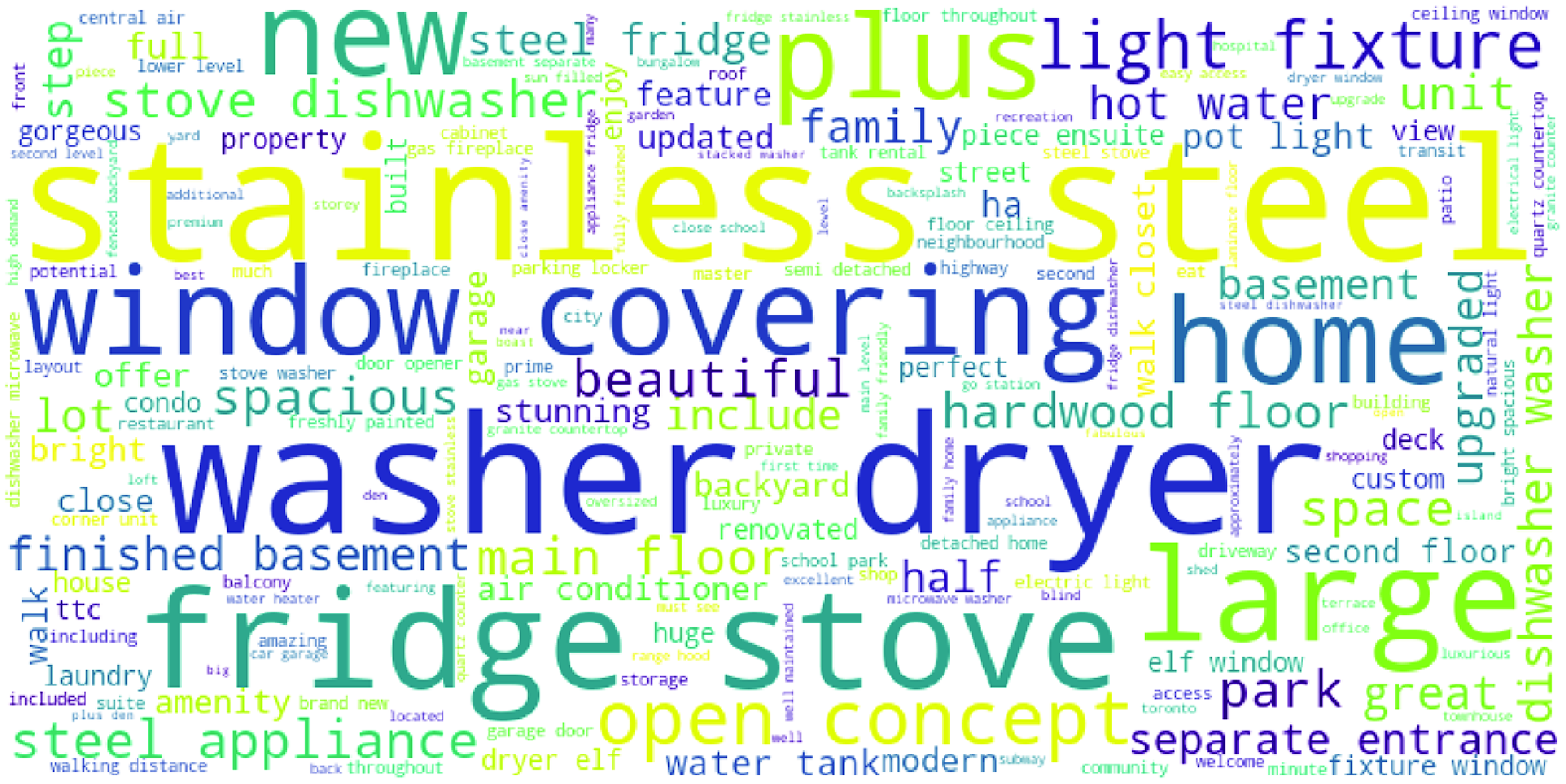
Figure 10. Word Cloud generated using the textual description data from the houses with average price.
3.2.5. Visualization of house textual description data
This section displays a small summary of the textual description data collected. Figures 8–10 show the word clouds obtained from different clusters of textual description data. Figure 8 shows the most frequent words that are present in the houses with the 5% lowest prices. Figure 9 shows the most frequent words that are present in the houses with the 5% highest prices. Finally, Figure 10 shows the most common words that we can observe in the textual description data of the 10% houses that have a price near the overall average value. It is apparent that for different price ranges, the word clouds have very different characteristics. For example, the properties with the lowest price have “unit,” “large,” “condo” as the most frequent words, while the most expensive properties have “home,” “plus,” “private” as the most frequent words. For the average price properties, the words describing the appliances “stainless steel,” “washer,” “dryer” are the most frequent. It is interesting to observe that the focus of the textual description varies as the price changes, which indicates a potential relation between the house textual description and its price. Therefore, this shows the importance of also considering the textual description data when predicting the house prices. We must highlight that the potential bias present in the textual data is an aspect that needs to be considered. As we have mentioned, the textual descriptions of the houses were obtained from a text directed to potential buyers. This text is written by domain experts with a specific target: selling houses. Thus, specific characteristics may have been highlighted to enhance the house quality. This means that some bias on the textual description may be included. We do not provide an analysis of this aspect, but we recognize that this might have some impact on the models built with this data. This aspect should be further investigated in future work.
4. Materials and methods
In this section, we describe the experiments carried out and the results obtained. We start by describing the word embedding methods used for the house textual description data. We present the experimental setup, including a description of the machine learning algorithms selected and performance assessment metrics estimated. Finally, we present and discuss the results obtained.
4.1. Word embedding for house listing description
Textual data need to be converted into numerical vectors using word embedding techniques so that machine learning algorithms can use them as input. We selected the following word embedding techniques for our experiments: TF-IDF, Word2Vec, and BERT.
TF-IDF provides a notion of how important a particular word is in a given document. To achieve this, the TF-IDF increases as the word frequency increases, while adjusting these results to take into account that some words have an overall higher frequency that is not necessarily associated with a higher importance of the word. This is a widely used and popular technique, as confirmed, for instance, by Beel et al. (Reference Beel, Gipp, Langer and Breitinger2016), who showed that the TF-IDF technique is widely used in recommender systems based on text in the context of digital libraries. To implement TF-IDF word embedding, we used the function TF-IDF Vectorizer in the Sklearn package to convert the textual description to TF-IDF values (Pedregosa et al. Reference Pedregosa, Varoquaux, Gramfort, Michel, Thirion, Grisel, Blondel, Prettenhofer, Weiss, Dubourg, Vanderplas, Passos, Cournapeau, Brucher, Perrot and Duchesnay2011). The words that have appeared in less than 3% of all the documents are ignored because these words could be part of an address or name that does not have significant meanings. In addition, the words that have appeared in more than 95% of all the documents are ignored as well, since these words are too common and do not help the model learn from the data. By setting the frequency threshold lower than 3% and higher than 95%, we can also significantly reduce embedding space from $\mathbb{R}^{15,280 \times d}$
to
$\mathbb{R}^{15,280 \times d}$
to $\mathbb{R}^{412 \times d}$
, thus alleviating computation cost in the overall process.Footnote
g
After the application of the TF-IDF Vectorizer, we obtained 412 words with the corresponding TF-IDF values. This will serve as the input for the regression algorithms. The list of the 412 words obtained for our study is provided at https://github.com/hansonchang2008/house-price-prediction-web-app/.
$\mathbb{R}^{412 \times d}$
, thus alleviating computation cost in the overall process.Footnote
g
After the application of the TF-IDF Vectorizer, we obtained 412 words with the corresponding TF-IDF values. This will serve as the input for the regression algorithms. The list of the 412 words obtained for our study is provided at https://github.com/hansonchang2008/house-price-prediction-web-app/.
The second technique we used is Word2Vec embedding. We used the Continuous Skip-gram architecture to train the Word2Vec embedding with all the collected house textual description data. The Skip-gram is a technique that stores n-grams in order to model the language. However, it allows to “skip” some tokens (Mikolov et al. Reference Mikolov, Chen, Corrado and Dean2013). We used the implementation of this architecture provided through the Gensim package (Rehurek and Sojka Reference Rehurek and Sojka2010). The target dimension of the word vectors is set to 300, which means that each word is converted into a 300-dimensional numerical vector. The window size is set to 8, which means the largest distance between the word to be analyzed and its neighboring words is 8. The minimum number of occurrences for a word to be considered is 1, and the number of training iterations is 30. We set these values after some preliminary tests. Finally, we transform each token in the textual description into a vector using the pre-trained Word2Vec. Then, we obtain the sentence embedding by calculating the mean pooling of all token embeddings from each specific sentence. This allows us to obtain the required sentence’s embedding by averaging over the previously obtained word vectors.
In addition to the pre-trained Word2Vec word embedding (which is trained using our target application data), we also experimented with other popular pre-trained word embedding models, including the Word2Vec and GloVe models. Word2Vec models include Google News and Fast Text. Regarding the GloVe model, Global Vectors for Word Representation model, we used their pre-trained models, that include Glove Wiki and Gigaword, and Glove Twitter word embedding. They were all implemented using the Gensim package (Rehurek and Sojka Reference Rehurek and Sojka2010).
We have run experiments on the converted word vectors to check the performance of all the word embedding models mentioned above. We used a single model to test the performance of these word embedding models: the GB regressor (Friedman Reference Friedman2001). We selected this learner as it is a well-known ensemble of trees that has shown good results in other tasks. We used the Scikit Learn package implementation of the GB regressor with default parameters. The performance estimation was carried out with 4 repetitions of 10-fold cross-validation on 90% of all data.
Table 4. Word2Vec and GloVe model results with the mean value of 10-fold cross-validation over four runs.

Table 4 shows the results obtained in this experiment. We observe that the self-trained continuous Skip-gram model clearly outperforms all the remaining 5 pre-trained Word2Vec and GloVe models regarding $R^2$
score and root mean squared error (
$R^2$
score and root mean squared error ( $\text{RMSE}$
). We carried out statistical significance test to confirm these results. The Friedman test results are reported in Table 4, and the Nemenyi post hoc test results are depicted in Figure 11.Footnote
h
There was a significant difference between the self-trained continuous Skip-gram model and both the Fasttext and GloVe-Twitter models. There was not a significant difference between the other groups of models. These results are consistent for both the
$\text{RMSE}$
). We carried out statistical significance test to confirm these results. The Friedman test results are reported in Table 4, and the Nemenyi post hoc test results are depicted in Figure 11.Footnote
h
There was a significant difference between the self-trained continuous Skip-gram model and both the Fasttext and GloVe-Twitter models. There was not a significant difference between the other groups of models. These results are consistent for both the $R^2$
score and the
$R^2$
score and the $\text{RMSE}$
. Note that the higher the
$\text{RMSE}$
. Note that the higher the $R^2$
score, the better the performance, while the lower the
$R^2$
score, the better the performance, while the lower the $\text{RMSE}$
, the better the performance.
$\text{RMSE}$
, the better the performance.
We believe that these results may be due to the fact that the Word2Vec model trained on the house textual description data has embedded more real estate industry-specific knowledge and thus achieved a better performance. As a result, we selected the self-trained continuous Skip-gram among the tested Word2Vec models. This is the only Word2Vec model we will use in the predictive model training and testing for the house price.
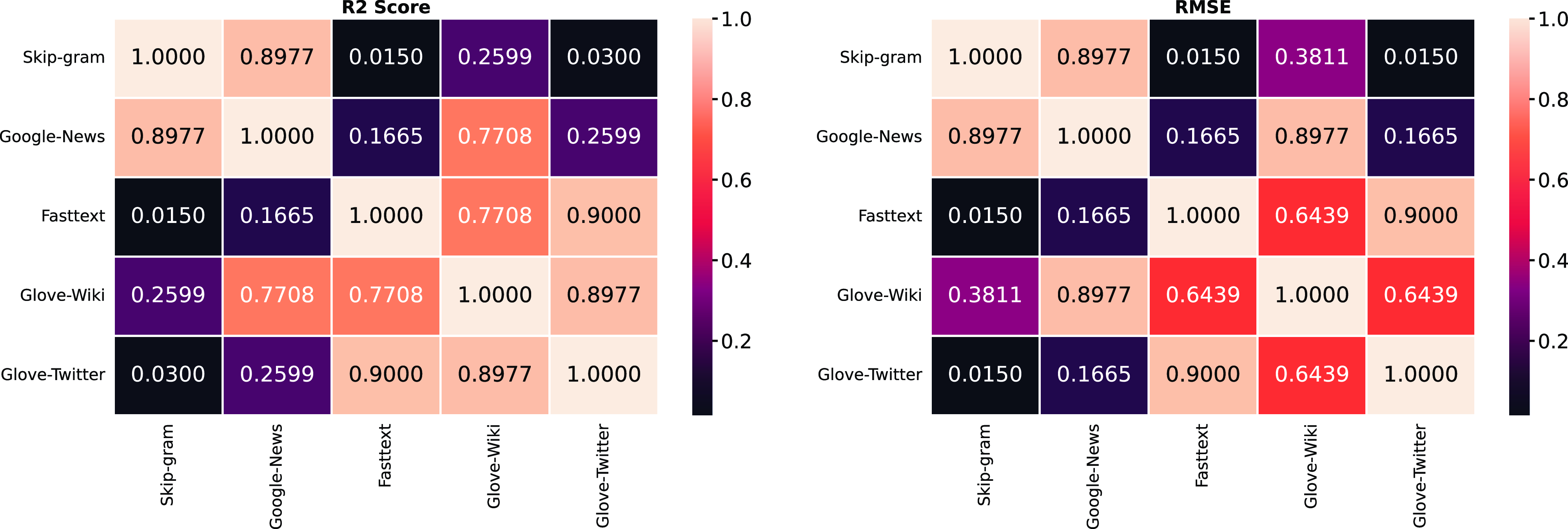
Figure 11. Nemenyi post hoc test of word embedding models with the mean of four repetitions of 10-fold cross-validation.
Finally, we also use BERT (Devlin et al. Reference Devlin, Chang, Lee and Toutanova2018) as an encoder of the textual description to obtain a set of features. To maximize the efficiency of the experiments, the pre-trained BERT base model is used to convert words into numerical feature vectors. The BERT model parameters are not changed, as this model is only used as a feature extractor to convert words into numerical vectors. The BERT model converts each house textual description into a numerical vector with a dimension of 768. The BERT base model is implemented using the transformers package (Wolf et al. Reference Wolf, Chaumond, Debut, Sanh, Delangue, Moi, Cistac, Funtowicz, Davison, Shleifer, von Platen, Ma, Jernite, Plu, Xu, Le Scao, Gugger, Drame, Lhoest and Rush2020).
4.2. Experimental setting
The main goal of our experiments is to determine the best algorithm to use to predict the asking house price while studying the use of different types of features for building the model. We want to understand if using the house textual description data has advantages and if the advantages vary for the different predictive models. To this end, we trained and tested four algorithms, using the described word embedding strategies, on three different feature subsets of the dataset: using only the features extracted from the textual description data, using only the other features without the textual description data, and using all the features extracted.
Table 5. Grid search parameters and values

DNN, deep neural network; GB, gradient boosting; L-SVR, linear support vector regression; RF, random forest.
When only textual description data is used, the output word vectors converted from description text would serve as the input for the algorithms. When all the textual description data and non-textual description data are used, the word vectors converted from the textual description data would be concatenated with the preprocessed non-textual description data and serve as the input features to the algorithm.
The four learning algorithms selected for this task are support vector regression (SVR), RF, GB, and DNN. All the algorithm parameters tested and tuned in our grid search are displayed in Table 5. This table shows the algorithms, parameters, and their values and provides a brief explanation regarding each parameter in each algorithm. For all the parameters that are not mentioned in Table 5, we used the default values in their corresponding algorithm implementation.
For the SVR, we selected the linear kernel. The motivation for this choice is that, in preliminary studies, non-linear kernels had an unsatisfactory performance. In these preliminary experiments, we observed that when using non-linear kernels, including “rbf,” “poly,” and “sigmoid” (Pedregosa et al. Reference Pedregosa, Varoquaux, Gramfort, Michel, Thirion, Grisel, Blondel, Prettenhofer, Weiss, Dubourg, Vanderplas, Passos, Cournapeau, Brucher, Perrot and Duchesnay2011), the $R^2$
score is always lower than 0, which means the model failed to learn from the textual description word vector data. For this reason, we did not apply them in this study. SVR with linear kernel was applied using the LinearSVR function in Scikit Learn package (Pedregosa et al. Reference Pedregosa, Varoquaux, Gramfort, Michel, Thirion, Grisel, Blondel, Prettenhofer, Weiss, Dubourg, Vanderplas, Passos, Cournapeau, Brucher, Perrot and Duchesnay2011).
$R^2$
score is always lower than 0, which means the model failed to learn from the textual description word vector data. For this reason, we did not apply them in this study. SVR with linear kernel was applied using the LinearSVR function in Scikit Learn package (Pedregosa et al. Reference Pedregosa, Varoquaux, Gramfort, Michel, Thirion, Grisel, Blondel, Prettenhofer, Weiss, Dubourg, Vanderplas, Passos, Cournapeau, Brucher, Perrot and Duchesnay2011).
For the RF algorithm, we used the RandomForestRegressor function available through the Scikit Learn package (Pedregosa et al. Reference Pedregosa, Varoquaux, Gramfort, Michel, Thirion, Grisel, Blondel, Prettenhofer, Weiss, Dubourg, Vanderplas, Passos, Cournapeau, Brucher, Perrot and Duchesnay2011). We varied four parameters in this algorithm as described in Table 5.
The regression version of GB was employed using the Scikit Learn function Gradient BoostingRegressor (Pedregosa et al. Reference Pedregosa, Varoquaux, Gramfort, Michel, Thirion, Grisel, Blondel, Prettenhofer, Weiss, Dubourg, Vanderplas, Passos, Cournapeau, Brucher, Perrot and Duchesnay2011). In this implementation, all base weak learners are decision trees. We varied four parameters for this learning algorithm.
Finally, we also used DNN models because this model is known for exhibiting good performance across multiple tasks and domains. The architecture of the DNN developed includes three hidden layers, two dropout layers, and one output layer. This architecture was implemented using the sequential model in the Keras package (Chollet et al. Reference Chollet2015). The number of neurons in each dense layer and their activation function are explained in Table 5. The output layer is a single node layer with a sigmoid activation function. The dropout layer is a regularization technique that prevents the DNN from overfitting by deactivating some percentage of the neurons randomly in the training process. We used the Adam optimizer (Kingma and Ba Reference Kingma and Ba2014), which typically outperforms other optimizers and shows good results. The loss function and the performance metric during training are both mean squared error ( $\text{MSE}$
).
$\text{MSE}$
).
Our experiments are run on a Windows 10 PC, with 16.0 GB of RAM, Intel Core i7-9750H CPU, and a NVIDIA GeForce RTX 2060 GPU. A storage space of 2 GB is needed for the data. To install the software, Anaconda version 2021.05 with Python 3 is needed. The code is Python code in Jupyter Notebook format. The following packages are also required: Scikit learn version 0.24.1, Pandas version 1.2.4, Gensim version 3.8.3, TensorFlow version 2.3.0, and Keras version 2.4.3. For reproducibility purposes, the code for all the experiments is freely available on GitHub at https://github.com/hansonchang2008/house-price-prediction-web-app/.
After finishing the data preprocessing, we have a total of 10,251 house listings in the dataset. The dataset is randomly split into two parts, 90% is used as the training data, and the remaining 10% is used as the testing data. Our first setup is to determine the best hyperparameters of the algorithms tested using a grid search procedure. In the grid search, we used only the training data and applied four repetitions of 10-fold cross-validation to estimate the performance and determine the best hyperparameters. To implement this, GridSearchCV of the Scikit Learn package was used (Pedregosa et al. Reference Pedregosa, Varoquaux, Gramfort, Michel, Thirion, Grisel, Blondel, Prettenhofer, Weiss, Dubourg, Vanderplas, Passos, Cournapeau, Brucher, Perrot and Duchesnay2011).
Overall, we assessed the performance on 28 combinations of problems: four regression algorithms were tested on three types of input data, with two of these having three different word embeddings applied. The first type of input uses only non-textual description data, which includes numerical, Boolean, and categorical data as previously described in Subsection 3.2.1. In this case, we do not consider a specific word embedding technique because no text data are involved. The non-textual description data are directly fed into the four regression algorithms. The second type of data is the textual description data. In this case, the textual description data are converted into word vectors by one of the three possible word embedding techniques described. Each one of the word vectors is then fed into the four regression algorithms. The third type of input data is to use all the features available. This includes both non-textual description data and textual description data. Non-textual description data are concatenated with one of the three word vectors obtained from the textual description data and then fed into the four regression algorithms.
In terms of the performance evaluation metrics, we evaluated both the $R^2$
score and the
$R^2$
score and the $\text{RMSE}$
. These metrics were applied to each configuration tested. To select the best set of hyperparameters for the learning algorithms,
$\text{RMSE}$
. These metrics were applied to each configuration tested. To select the best set of hyperparameters for the learning algorithms, $R^2$
is used. Equations (1) and (2) provide the formulas for computing both performance assessment metrics. In these equations,
$R^2$
is used. Equations (1) and (2) provide the formulas for computing both performance assessment metrics. In these equations, $y_i$
represents the true target variable value,
$y_i$
represents the true target variable value, $f_i$
represents the predicted target variable value,
$f_i$
represents the predicted target variable value, $\bar{y}$
is the average of the target variable value, and
$\bar{y}$
is the average of the target variable value, and $n$
is the total number of listings.
$n$
is the total number of listings.
 \begin{equation} R^2 = 1-\frac{\sum _{i=1}^n (y_i-f_i)^2}{\sum _{i=1}^n (y_i-\bar{y})^2} \end{equation}
 \begin{equation} \text{RMSE}=\sqrt{\frac{\sum _{i=1}^n (f_i-y_i)^2}{n}} \end{equation}
4.3. Results and discussion
This section presents the results obtained in our experiments. We begin by displaying the grid search results which were obtained based on the training data. These results allow us to determine the best parameters for the learning algorithms. Then, we use the $\text{RMSE}$
results to select the best combination of learning algorithm and word embedding strategy for each of the three possible types of data input (non-textual description data, textual description data, all features). The selected combination is applied to obtain the results on the test set.
$\text{RMSE}$
results to select the best combination of learning algorithm and word embedding strategy for each of the three possible types of data input (non-textual description data, textual description data, all features). The selected combination is applied to obtain the results on the test set.
4.3.1. Grid search results
Regarding the grid search results, the best validation $R^2$
score and
$R^2$
score and $\text{RMSE}$
score for all settings are shown in Tables 6 and 7, respectively. The determined sets of best parameters for each setting are provided in the Appendix in Table A1.
$\text{RMSE}$
score for all settings are shown in Tables 6 and 7, respectively. The determined sets of best parameters for each setting are provided in the Appendix in Table A1.
Table 6. Best $R^2$
scores for all algorithms
$R^2$
scores for all algorithms

DNN, deep neural network; GB, gradient boosting; L-SVR, linear support vector regression; RF, random forest. Best result per each feature set considered in bold and second-best underlined.
Table 7. Best $\text{RMSE}$
scores for all algorithms
$\text{RMSE}$
scores for all algorithms

DNN, deep neural network; GB, gradient boosting; L-SVR, linear support vector regression; RF, random forest. Best result per each feature set considered in bold and second-best underlined.
We begin the analysis of the grid search results by considering each input feature set: only non-textual description data, only textual description data, and both (textual and non-textual description data). When using non-textual description features only, which are the frequently used features in the traditional house prediction model, we observe that RF and GB are the best-performing algorithms when considering $\text{RMSE}$
and
$\text{RMSE}$
and $R^2$
scores, respectively. In this case, the DNN ranks third, while the linear SVR is the worst-performing model. We observe that the deep learning model we selected did not perform well in this case, which we hypothesize to be potentially related to the architecture selected.
$R^2$
scores, respectively. In this case, the DNN ranks third, while the linear SVR is the worst-performing model. We observe that the deep learning model we selected did not perform well in this case, which we hypothesize to be potentially related to the architecture selected.
When all features are used to build a model, we found that the best solution is the GB regression algorithm with TF-IDF word embedding. This gives the highest $R^2$
score of 0.7214 and the lowest
$R^2$
score of 0.7214 and the lowest $\text{RMSE}$
score of 0.0192. The addition of textual description data provides an increase of 5.9% over the baseline GB model with no textual description data when the
$\text{RMSE}$
score of 0.0192. The addition of textual description data provides an increase of 5.9% over the baseline GB model with no textual description data when the $R^2$
score is considered. GB performs better than any other regression algorithms, regardless of the word embedding option, with the exception of DNNs with Word2Vec embedding, which exhibits an
$R^2$
score is considered. GB performs better than any other regression algorithms, regardless of the word embedding option, with the exception of DNNs with Word2Vec embedding, which exhibits an $R^2$
score of 0.7029.
$R^2$
score of 0.7029.
It is also important to notice that the worst-performing regression algorithm is linear SVR, which is significantly outperformed by the other three regression algorithms. We hypothesize that the linear SVR’s lowest complexity when compared against the other algorithms explains why this solution is not able to model the non-linearity of the problem well.
In addition, for the setting where all features are used, we observe that DNN models rank second while RF models rank third in terms of performance. An interesting outcome from the evaluation using all features is that for RF, adding the textual description data to the non-textual description input data does not impact the model’s performance. This is also the case with the GB algorithm with Word2Vec or BERT. We hypothesize that a possible information overlap between non-textual description features and the house description text can be a possible explanation for this outcome. For example, the building type “condo” is one of the non-textual description features that can also be included in the house description text. We would like to highlight that using both textual and non-textual description data generally provides performance improvements. A deeper investigation of the impact of the different features in these cases needs to be carried out. Moreover, an assessment of the features’ importance carried out for the different learning algorithms can also be beneficial to understand how they are impacted by the features.
Our final analysis concerns the performance assessment of the models that only use textual description data. DNN model with Word2Vec word embedding stands out in this case by generating the highest $R^2$
score of 0.6041 and the lowest
$R^2$
score of 0.6041 and the lowest $\text{RMSE}$
score of 0.0220. We observe that when learning only from the textual description data, the solutions using deep learning provide the best results showing a good fit for this task. Using house description text alone produces an
$\text{RMSE}$
score of 0.0220. We observe that when learning only from the textual description data, the solutions using deep learning provide the best results showing a good fit for this task. Using house description text alone produces an $R^2$
score 28.77% higher than using only non-textual description features in this setting. This shows that the description text itself is a powerful predictive feature. The GB model with Word2Vec word embedding is the second best-performing model with an
$R^2$
score 28.77% higher than using only non-textual description features in this setting. This shows that the description text itself is a powerful predictive feature. The GB model with Word2Vec word embedding is the second best-performing model with an $R^2$
score of 0.5219. This shows that the self-trained Word2Vec word embedding is a powerful tool to extract features from the house description text. An interesting finding is that DNN performs better than any other regression algorithm when compared based on the same word embedding technique. However, we must highlight that the best performance achieved when using only textual description data is still worse than the one achieved when using both textual and non-textual description data.
$R^2$
score of 0.5219. This shows that the self-trained Word2Vec word embedding is a powerful tool to extract features from the house description text. An interesting finding is that DNN performs better than any other regression algorithm when compared based on the same word embedding technique. However, we must highlight that the best performance achieved when using only textual description data is still worse than the one achieved when using both textual and non-textual description data.
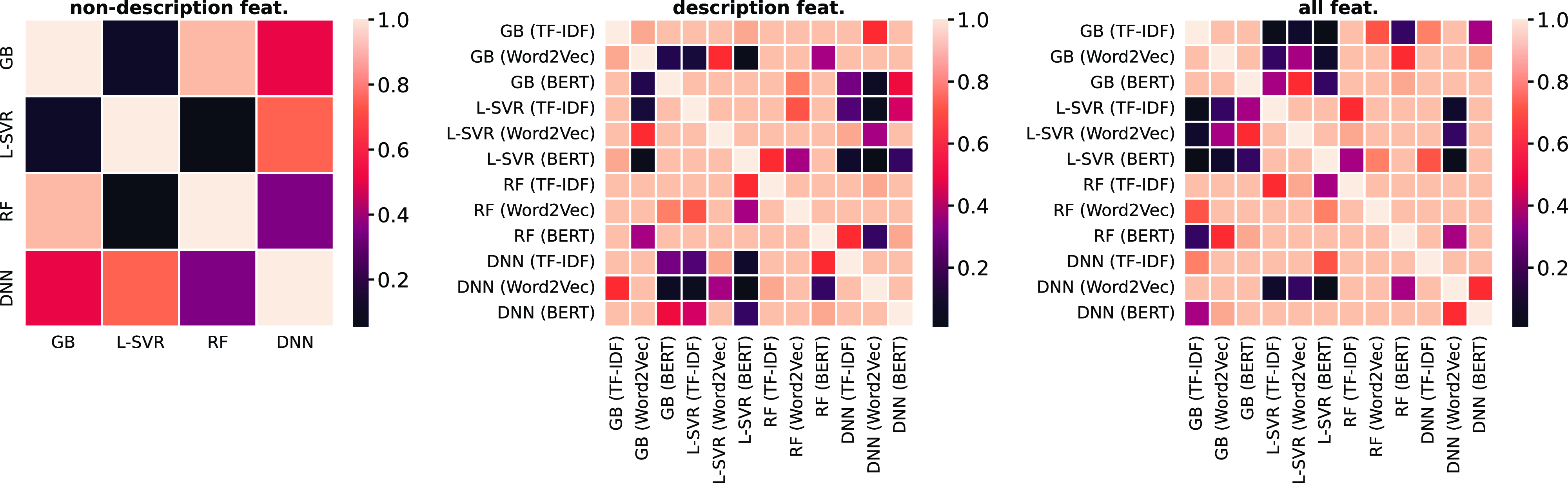
Figure 12. Nemenyi post hoc test of $R^2$
scores for all algorithms with the mean of four repetitions of 10-fold cross-validation.
$R^2$
scores for all algorithms with the mean of four repetitions of 10-fold cross-validation.
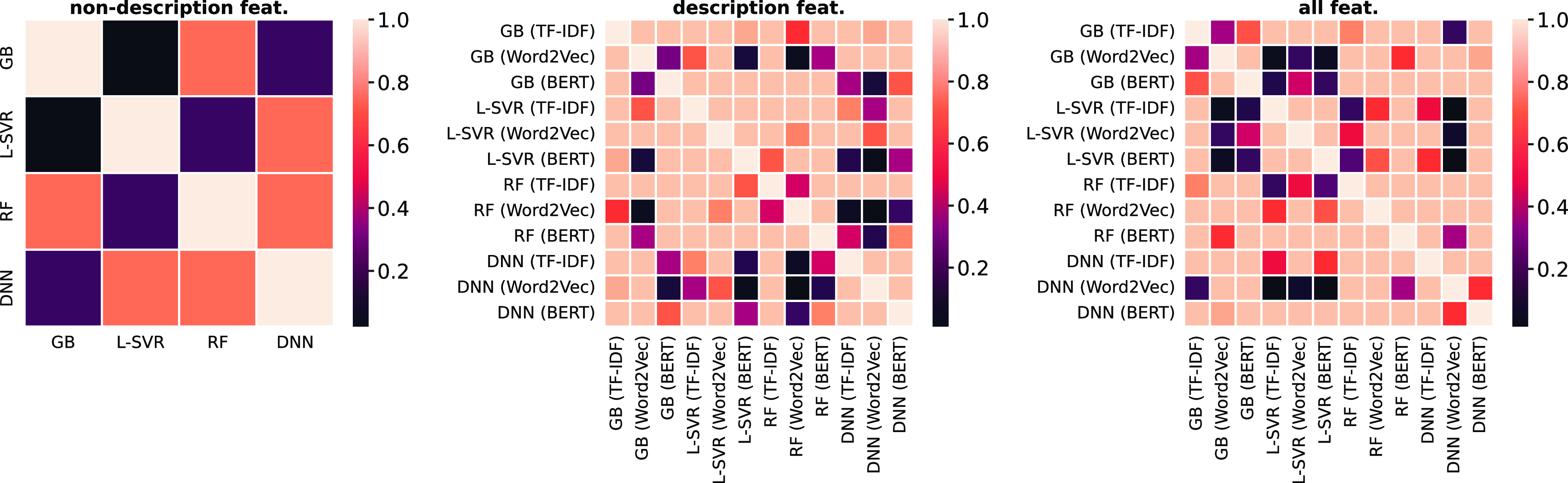
Figure 13. Nemenyi post hoc test of $\text{RMSE}$
scores for all algorithms with the mean of four repetitions of 10-fold cross-validation.
$\text{RMSE}$
scores for all algorithms with the mean of four repetitions of 10-fold cross-validation.
In terms of the statistical significance, we observed the Friedman Test and then applied the Nemenyi post hoc test that is shown in Figure 12 for the $R^2$
score and in Figure 13 for the
$R^2$
score and in Figure 13 for the $\text{RMSE}$
.Footnote
i
These two figures are displayed in the appendix with the color scheme and the corresponding p-value. We observe that there was a significant difference between the SVR and RF for
$\text{RMSE}$
.Footnote
i
These two figures are displayed in the appendix with the color scheme and the corresponding p-value. We observe that there was a significant difference between the SVR and RF for $R^2$
and between SVR and GB for
$R^2$
and between SVR and GB for $\text{RMSE}$
, when applying models that use non-textual description features. For the models that use textual description features, there was a significant difference between the DNN with TF-IDF and SVR with BERT; SVR with BERT and GB with Word2Vec; and between DNN with Word2Vec and the following models: GB with BERT, SVR with TF-IDF, SVR with BERT for the
$\text{RMSE}$
, when applying models that use non-textual description features. For the models that use textual description features, there was a significant difference between the DNN with TF-IDF and SVR with BERT; SVR with BERT and GB with Word2Vec; and between DNN with Word2Vec and the following models: GB with BERT, SVR with TF-IDF, SVR with BERT for the $R^2$
. For the
$R^2$
. For the $\text{RMSE}$
there was a significant difference between the following models: RF with Word2Vec and GB with Word2Vec; DNN with TF-IDF and RF with Word2Vec; and, DNN with Word2Vec and both SVR with BERT, RF with Word2Vec. Finally, for the models using all features there was a significant difference between the following groups for the
$\text{RMSE}$
there was a significant difference between the following models: RF with Word2Vec and GB with Word2Vec; DNN with TF-IDF and RF with Word2Vec; and, DNN with Word2Vec and both SVR with BERT, RF with Word2Vec. Finally, for the models using all features there was a significant difference between the following groups for the $R^2$
score: all three SVR models and the GB with TF-IDF; SVR with BERT and GB with Word2Vec; and DNN with Word2Vec and SVR with both TF-IDF and BERT. For the
$R^2$
score: all three SVR models and the GB with TF-IDF; SVR with BERT and GB with Word2Vec; and DNN with Word2Vec and SVR with both TF-IDF and BERT. For the $\text{RMSE}$
and the models using all features, there was a significant difference between the following groups: SVR, with both BERT and TF-IDF, and BG with Word2Vec; and DNN with Word2Vec and the three SVR models.
$\text{RMSE}$
and the models using all features, there was a significant difference between the following groups: SVR, with both BERT and TF-IDF, and BG with Word2Vec; and DNN with Word2Vec and the three SVR models.
We also analyze the results from the perspective of the applied word embedding technique to observe its potential impact on the performance. When only the textual description features are used, the Word2Vec word embedding shows the best performance among the three, followed by TF-IDF. The Word2Vec shows the best improvement over TF-IDF in GB, where Word2Vec outperforms the TF-IDF by 43.54% in the $R^2$
score. When all the features are used, Word2Vec and TF-IDF are both the best for word embedding, and there is no clear winner. For GB and RF, TF-IDF gives the best
$R^2$
score. When all the features are used, Word2Vec and TF-IDF are both the best for word embedding, and there is no clear winner. For GB and RF, TF-IDF gives the best $R^2$
score. However, for linear SVR and DNN, Word2Vec performs the best.
$R^2$
score. However, for linear SVR and DNN, Word2Vec performs the best.
Overall, BERT is the worst-performing word embedding technique. In fact, this technique consistently displays the worst scores for both $R^2$
and
$R^2$
and $\text{RMSE}$
when compared against the TF-IDF and Word2Vec techniques. We hypothesize that this may be due to the fact that, in our experiments, TF-IDF and Word2Vec both have been trained using the domain description textual data, while BERT is a pre-trained model trained on different textual data. This seems to indicate that these two techniques are able to help achieve a better understanding of the language used in the real estate industry. In comparison, the BERT model is pre-trained on two broad corpora of Wikipedia and BooksCorpus documents, which may explain BERT’s difficulty understanding well the vocabulary meaning within the specific real estate industry.
$\text{RMSE}$
when compared against the TF-IDF and Word2Vec techniques. We hypothesize that this may be due to the fact that, in our experiments, TF-IDF and Word2Vec both have been trained using the domain description textual data, while BERT is a pre-trained model trained on different textual data. This seems to indicate that these two techniques are able to help achieve a better understanding of the language used in the real estate industry. In comparison, the BERT model is pre-trained on two broad corpora of Wikipedia and BooksCorpus documents, which may explain BERT’s difficulty understanding well the vocabulary meaning within the specific real estate industry.
4.3.2. Final models’ results and discussion
Based on the results obtained from the grid search (in Tables 6 and 7), we selected the best algorithm with the best set of parameters to build the final model for each of the 3 feature sets: only textual description data, only non-textual description data, and both. For each type of input data, one algorithm is selected to build one model. GB is selected as the best algorithm for non-textual description features because it has the lowest $\text{RMSE}$
among all the regression algorithms. For textual description data input, the best approach is a DNN with Word2Vec word embedding. When we consider all the features, GB with TF-IDF word embedding has the best performance. The three algorithms and their best set of parameters are shown in Table 8.
$\text{RMSE}$
among all the regression algorithms. For textual description data input, the best approach is a DNN with Word2Vec word embedding. When we consider all the features, GB with TF-IDF word embedding has the best performance. The three algorithms and their best set of parameters are shown in Table 8.
Table 8. Best algorithms and the best parameters for all three input data types.

DNN, deep neural network; GB, gradient boosting.
After determining the best combination of approaches, we use the entire training data available to build a model. This will allow us to efficiently take advantage of all the data to build a more robust model that can achieve the best performance. Thus, the three built final models are trained with the algorithms and parameters as shown in Table 8 using the entire training data available. These models are then evaluated based on the testing data.
The final models’ experimental results are shown in Table 9. We observe that Model 2, which was built using only textual description data, has achieved the highest testing $R^2$
score of 0.7904. This indicates that this model achieves a good relative fit for the data. The testing
$R^2$
score of 0.7904. This indicates that this model achieves a good relative fit for the data. The testing $\text{RMSE}$
score is the highest, which means the absolute fit for the data of the model is not as good as Model 1 or 3 under this metric perspective. When observing the relative fit of the models, we notice that Model 3, which uses all available features, gives the best testing
$\text{RMSE}$
score is the highest, which means the absolute fit for the data of the model is not as good as Model 1 or 3 under this metric perspective. When observing the relative fit of the models, we notice that Model 3, which uses all available features, gives the best testing $\text{RMSE}$
score and the second highest testing
$\text{RMSE}$
score and the second highest testing $R^2$
score. In comparison to Model 1 which only uses non-textual description features, it can be observed that Model 3 has better performance in terms of both
$R^2$
score. In comparison to Model 1 which only uses non-textual description features, it can be observed that Model 3 has better performance in terms of both $R^2$
and
$R^2$
and $\text{RMSE}$
scores. The testing
$\text{RMSE}$
scores. The testing $R^2$
score increases from 0.6738 to 0.7184, while the testing
$R^2$
score increases from 0.6738 to 0.7184, while the testing $\text{RMSE}$
score decreases from 0.0155 to 0.0144.
$\text{RMSE}$
score decreases from 0.0155 to 0.0144.
To provide a better understanding of the errors these models are making, we converted the results of test RMSE presented in Table 9 to the value in Canadian Dollars (CAD). Model 1 test RMSE error of 0.0155 corresponds to $\$$
86,037.55 CAD, Model 2 test RMSE error of 0.0238 corresponds to
$\$$
86,037.55 CAD, Model 2 test RMSE error of 0.0238 corresponds to $\$$
122,007.98 CAD, and Model 3 test RMSE error of 0.0144 corresponds to
$\$$
122,007.98 CAD, and Model 3 test RMSE error of 0.0144 corresponds to $\$$
72,234.24 CAD. It is clear that these values still need to be further improved. This indicates that the addition of the house textual description feature to the input features could improve the performance of the traditional model that only uses non-textual description features. The possible bias present in the textual description data can also be a factor to consider in these results. We observe that this data can be useful, but the consideration of the bias should be taken into account in the future. We hypothesize that the usage of unbiased textual description data can have a more positive impact on the models.
$\$$
72,234.24 CAD. It is clear that these values still need to be further improved. This indicates that the addition of the house textual description feature to the input features could improve the performance of the traditional model that only uses non-textual description features. The possible bias present in the textual description data can also be a factor to consider in these results. We observe that this data can be useful, but the consideration of the bias should be taken into account in the future. We hypothesize that the usage of unbiased textual description data can have a more positive impact on the models.
Table 9. Result for final models.

DNN, deep neural network; GB, gradient boosting.
4.3.3. Experimental results summary
This section summarizes the thorough analysis carried out. Our main findings are as follows:
the best performance is achieved when using both textual and non-textual description data;
RF and GB are the best models to use when we consider only non-textual description data;
GB was the best-performing model when both textual and non-textual description data were taken into account;
deep learning models provide a performance advantage when learning only from textual description data;
on the final test set, the deep learning model with Word2Vec using only textual description data achieved the best performance in terms of $R^2$
;
$R^2$
;also on the final test set, when observing the
$\text{RMSE}$
, the best model was GB with TF-IDF as a word embedding technique using both textual and non-textual description features;the model using only non-textual description data from the final test set was never the best-performing model for the two metrics considered.


Overall, we observe that this is a complex problem that still needs further research to be carried out. The complexity and richness of the textual description data can be an interesting avenue to explore in the future. More attention should be given to the use of deep learning models, which explore more architectures and ways to extract useful features. Finally, the potential bias including the textual data should also be further investigated.
5. Web application developed
Making our developed model freely available to all interested users by deploying it on a website could help real estate sellers and buyers evaluate the house’s asking price using the description text. Moreover, this model can also help home sellers build texts that highlight features important for a targeted selling price. This way, it may help in finding house description texts targeting specific audiences. A web application has been developed to serve this purpose. The chosen model is Model 2, as determined in Section 4.3.2. We used the programming language Python and the Flask web framework in our implementation. Both are suitable for small-scale web application development. The developed web application is freely available at https://house-price-predict-dnn-model.herokuapp.com/. Moreover, a GitHub repository associated with the developed application, which also contains all the code developed in this paper, is also provided at the following link: https://github.com/hansonchang2008/house-price-prediction-web-app/.
The web application developed uses three model files. First, the DNN model trained with the description text input has been serialized to a model file. The second saved model is the MinMaxScaler used to normalize the price to the range of 0 and 1. Finally, the self-trained Word2Vec model is also saved. These three files will be used to obtain the predicted house price given the input text provided by the application user.
Figure 14 (on the left) displays the web application start page. Our web application works as follows. The user first enters the text containing the house description in the text box and presses the prediction button. Then, the web application does the preprocessing step for Word2Vec on the user input, uses the self-trained Word2Vec model to convert the description text into word vectors, and then applies the serialized deep learning model for prediction.
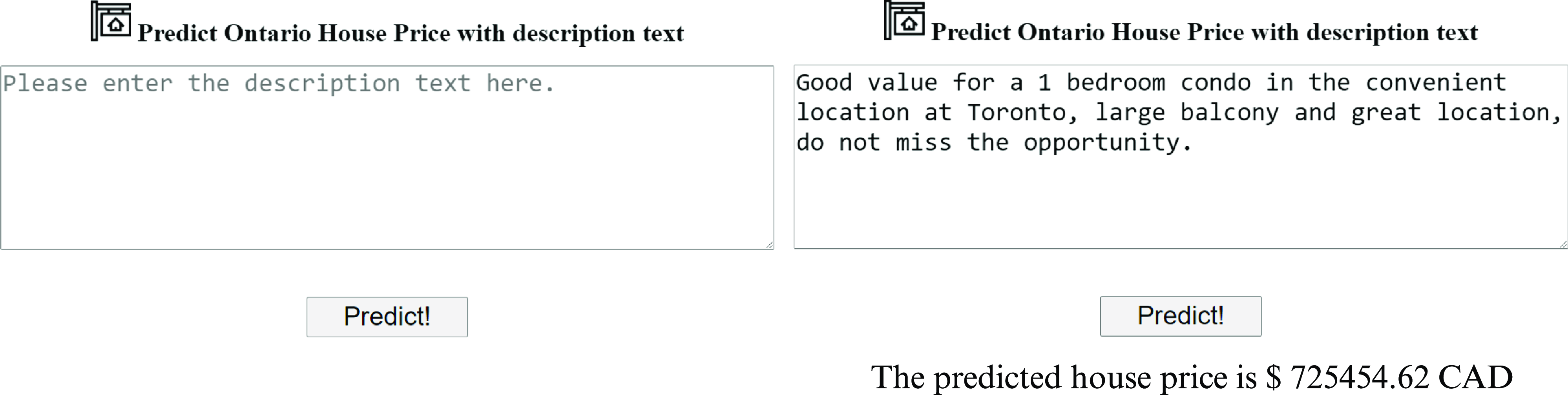
Figure 14. Web application initial page (left) and example of a price prediction for a 1-bedroom condo (right), using the developed App.
We refer to the previously trained and saved deep learning model as the serialized model. This is the best deep learning model that we obtained in our previous experiments and that we now reuse to obtain the new prediction for the text entered by the end-user. We use Python capabilities to extract this model and store it for reuse in the web application. We used Python’s pickle format for storing the model. The output of the model is the normalized house price. To show the user the non-normalized predicted house price, the MinMaxScaler model is used reversely with the inverse transform function to convert the normalized house price to the actual predicted house price. The final predicted house price is pushed to the website as the result is shown to the user. An example can be seen in Figure 14 (right-hand side), where a textual description text for a 1-bedroom condo in Toronto is inputted and the house’s predicted price is shown.
In the left-hand side of Figure 15, we provide the same input text for a house textual description that is provided in Figure 14 but change the city from Toronto to Ottawa. In this case, we observe that the model now predicts a lower price of about 603 thousand dollars. This is consistent with the fact that house prices in Ottawa are generally lower than in Toronto. We also show an example of entering a house listing textual description for a detached house that the buyer can customize. In this setting, the asking price predicted would be much higher than the previous example with a condo. This can be seen in Figure 15 on the right side, where the 3-bedroom house close to the river in Ottawa has a predicted asking price of $\$$
1.34 million. This reflects the fact that a 3-bedroom house is more expensive than a 1-bedroom condo in Ottawa.
$\$$
1.34 million. This reflects the fact that a 3-bedroom house is more expensive than a 1-bedroom condo in Ottawa.
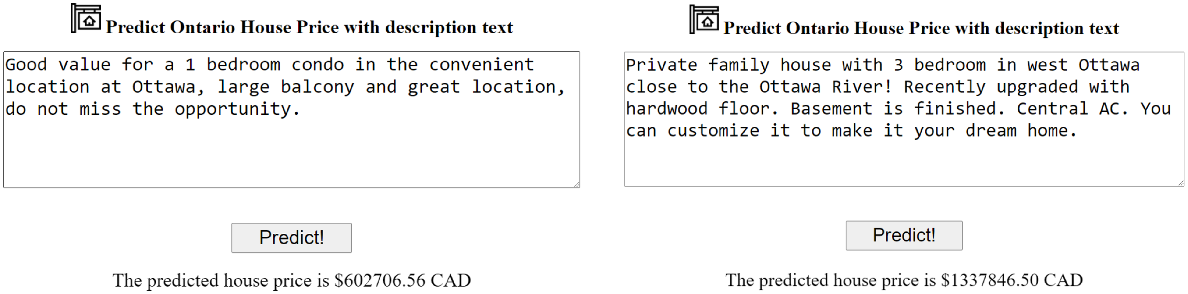
Figure 15. Price prediction for a 1-bedroom condo in Ottawa (left), and price prediction for a 3-bedroom house in Ottawa near the Ottawa River (right), using the developed App.
6. Conclusion
In this paper, we tackle the problem of predicting house prices by studying the use of different features, including textual and non-textual description data. In order to obtain a large set of real-world and updated examples, a web scraper was developed to collect data from a Canadian house listing website.
An extensive and detailed data cleaning and preprocessing were applied to obtain a high-quality dataset. We studied three different word embedding techniques. Thus, we applied data preprocessing procedures to the textual description data that were specially tailored to each one of the word embedding techniques.
Four regression algorithms were used in Grid Search. The result shows that for textual description data input, DNNs have the best performance when paired with Word2Vec word embedding. However, when all features are used, the GB algorithm is the best among the four when it is paired with the TF-IDF word embedding model. Linear support vector regressor is inferior in all criteria. Grid search results showed that the textual description data itself could be a strong predictor for the asking price of a house, where a high validation $R^2$
score of 0.6016 was produced by the DNN with the Word2Vec algorithm.
$R^2$
score of 0.6016 was produced by the DNN with the Word2Vec algorithm.
Our experiments strongly suggest that using both textual and non-textual description data can improve the performance of the majority of the regression models when compared to models that use only non-textual description data. When textual description data are used as input, Word2Vec embedding is the best strategy to use, followed by TF-IDF and then BERT. The BERT model is pre-trained on a large corpus. However, our research showed that even though BERT is known for having a generally good performance, this model might not be suitable for our specific problem with house textual description data. We hypothesize that this may be due to the fact that it is not trained on a real estate corpus and thus exhibits difficulties in this special scenario. Training a word embedding model on an industry-specific corpus may be vital for the learning of word associations.
Three final models are derived for the evaluation, each one corresponding to a type of input data. The testing results show that while the deep learning model using textual description input could produce the highest $R^2$
score, the
$R^2$
score, the $\text{RMSE}$
score obtained was not the best. This might be due to the fact that the model could have a very good relative fit on the data but not a very good absolute fit. Relative fit is more valuable than absolute fit in price prediction, for absolute price differences depend on the price range of a property as well.
$\text{RMSE}$
score obtained was not the best. This might be due to the fact that the model could have a very good relative fit on the data but not a very good absolute fit. Relative fit is more valuable than absolute fit in price prediction, for absolute price differences depend on the price range of a property as well.
Finally, a web application for house price prediction using description text has been developed and hosted on the Internet for free. This application is powered by the best-determined model that uses textual description data: the DNN model with Word2Vec word embedding. The web application has a simple design and an intuitive interface and is freely available to interested users and the research community.
In the future, we will further validate the generalizability of our proposed house price prediction model regarding different data sources (i.e., varying from different cities to different countries) as well as other datasets obtained by other researchers. Besides that, we also plan to explore the possibility of training some of the last layers in the BERT model and evaluate the performance. The development of a BERT model specialized in the particular context of texts describing houses could be interesting to explore. We will also carry out a comparative study using multiple different neural network architectures to deal with the textual description data in order to find which network works better in this problem domain. Moreover, we plan to conduct research on the use of GANs as an oversampling strategy and the usage of reinforcement learning as a feature selection strategy. The investigation of the bias in the textual description data collected from different sources is another interesting future research path. Comparing the impact on the performance of texts extracted from multiple websites, potentially containing different writing styles, and/or targeting different audiences is a relevant future work. Since the neural network is a black box, more algorithms could be explored for providing an explainability of the predicted values. For example, the neural network-based decision tree algorithm (Wan et al. Reference Wan, Dunlap, Ho, Yin, Lee, Jin, Petryk, Bargal and Gonzalez2020) could be studied to develop a machine learning prediction model with a high level of explainability. The problem of overfitting should also be investigated, and several tests should be carried out. We plan to include in the webapp not only more models but also several tools for the interpretability and explainability of the different models. The usage of this webapp as a tool for helping human annotators is a potentially interesting path to explore, especially if it is improved to include more explainability and interpretability of the results. Finally, another interesting research direction is related to the collection of house textual description data from multiple sources, which may provide a more diversified perspective of the houses and thus can lead to interesting outcomes.
Competing interests
The author(s) declare none.
Appendix A
Table A1 contains the results obtained on the best parameters found on the grid search carried out in Section 4.
Table A1. Detailed results of the algorithms and respective best parameter settings found through the grid search.
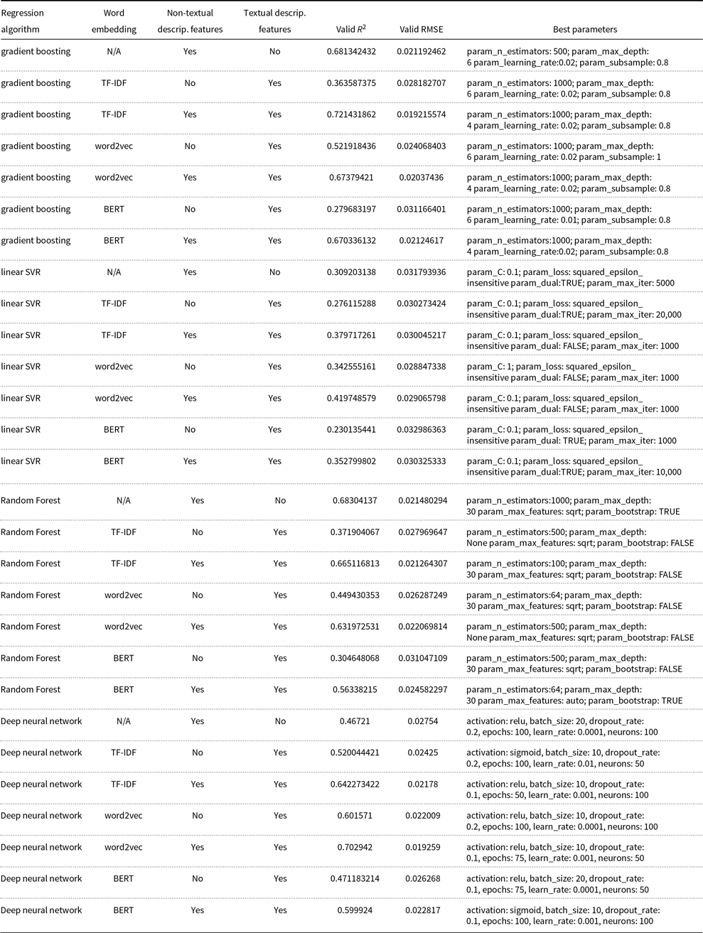
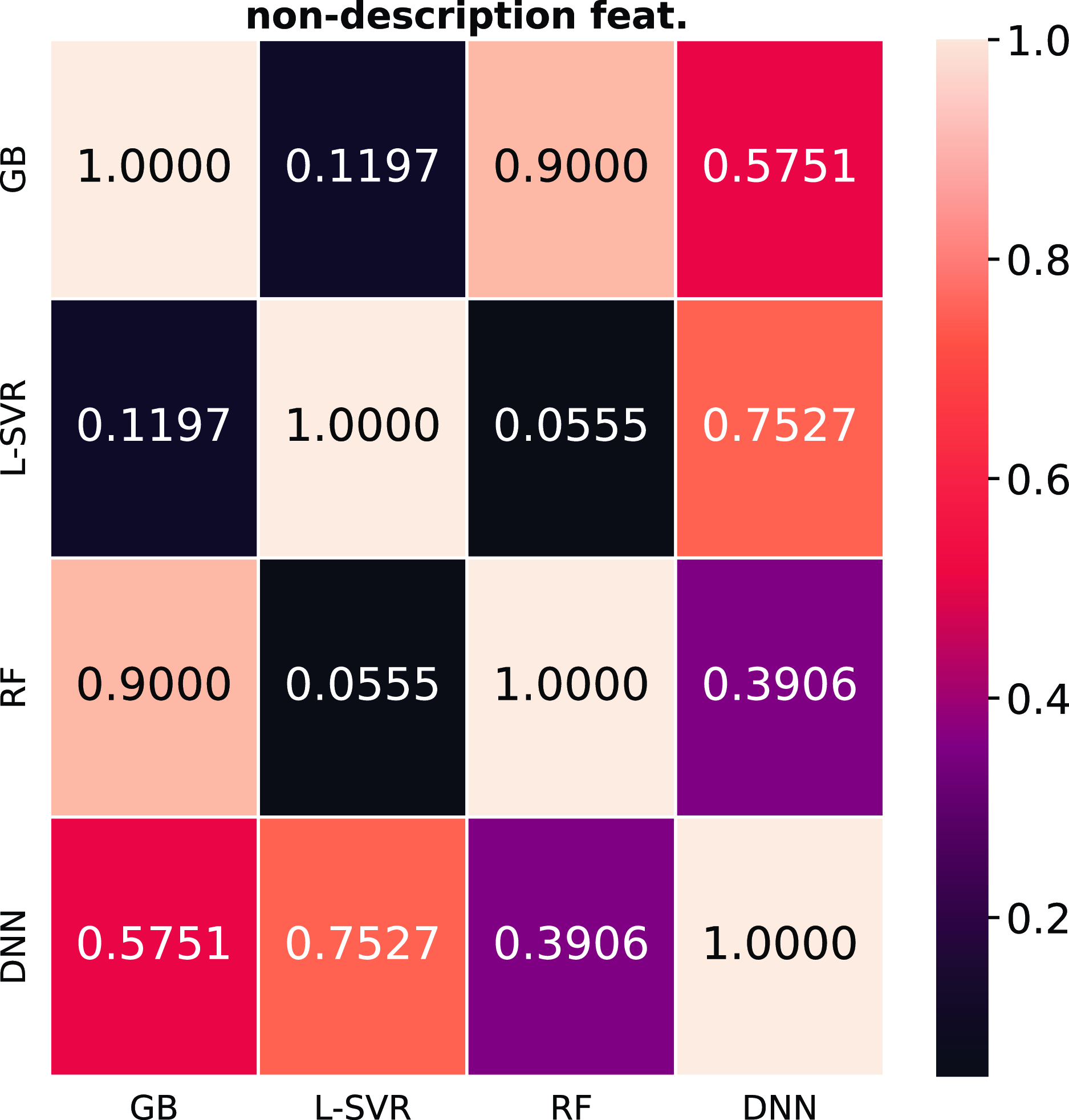
Figure A1. Nemenyi post hoc test of $R^2$
scores for non-textual description features.
$R^2$
scores for non-textual description features.
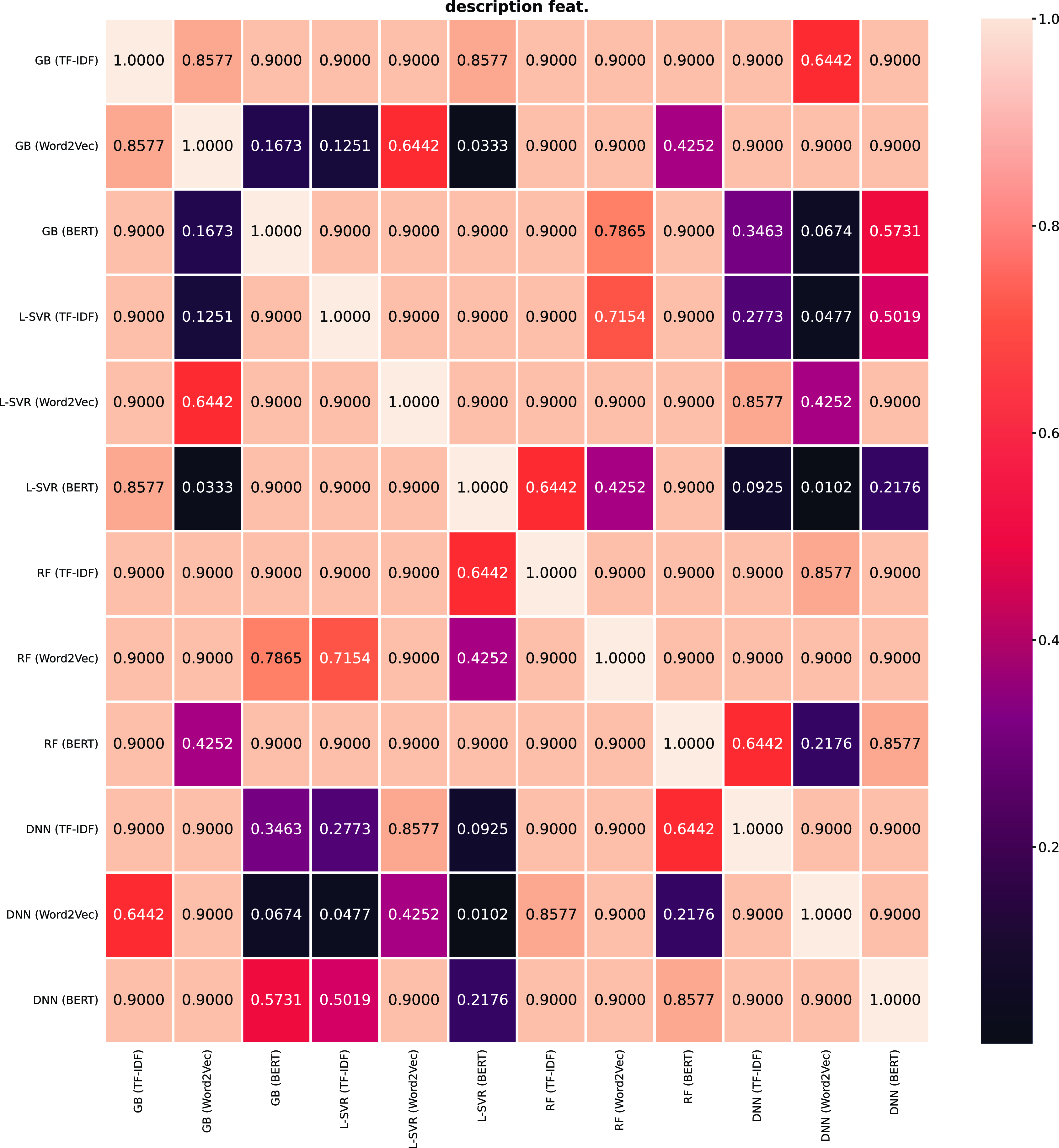
Figure A2. Nemenyi post hoc test of $R^2$
scores for textual description features.
$R^2$
scores for textual description features.

Figure A3. Nemenyi post hoc test of $R^2$
scores for all features.
$R^2$
scores for all features.
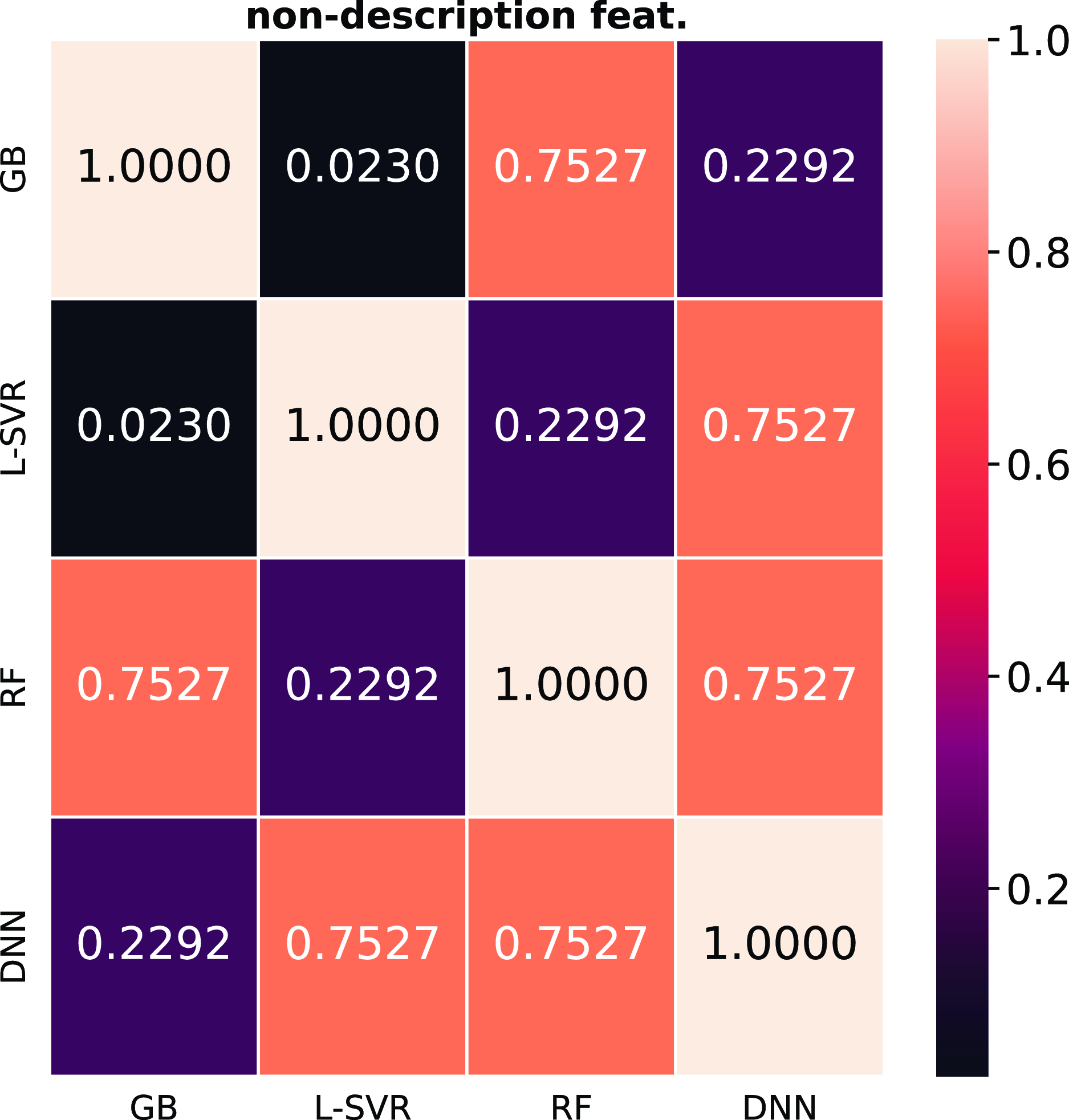
Figure A4. Nemenyi post hoc test of $\text{RMSE}$
scores for non-textual description features.
$\text{RMSE}$
scores for non-textual description features.
Figures A1–A3 show the results of the p-values of the Nemenyi Test carried out for the $R^2$
score considering only models using non-textual description features, textual description features, and all features, respectively. These three figures complement Figure 12 displayed in the main manuscript.
$R^2$
score considering only models using non-textual description features, textual description features, and all features, respectively. These three figures complement Figure 12 displayed in the main manuscript.
Figures A4–A6 show the results of the p-values of the Nemenyi Test carried out for the $\text{RMSE}$
considering only models using non-textual description features, textual description features, and all features, respectively. These three figures complement Figure 13 displayed in the main manuscript.
$\text{RMSE}$
considering only models using non-textual description features, textual description features, and all features, respectively. These three figures complement Figure 13 displayed in the main manuscript.
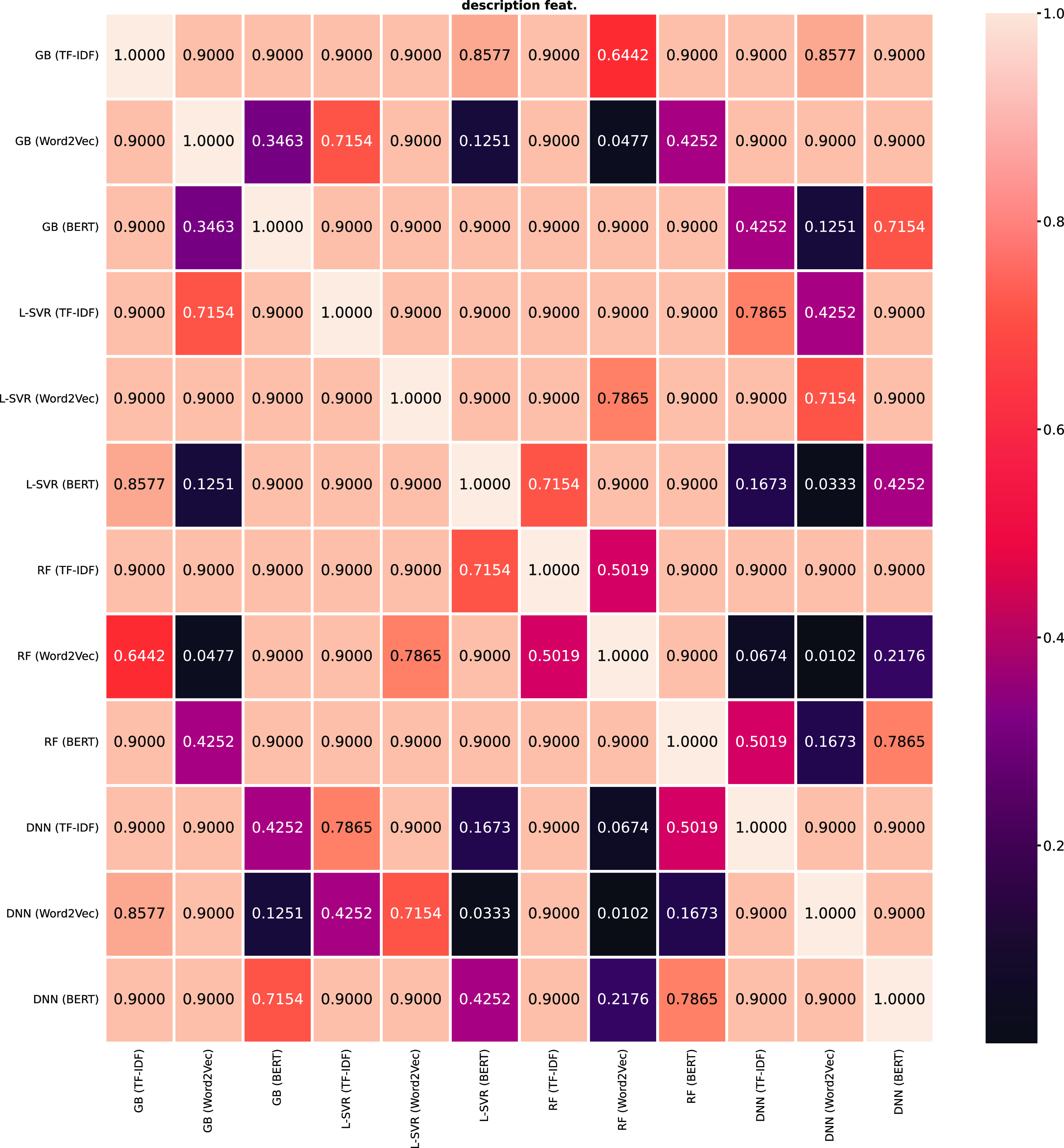
Figure A5. Nemenyi post hoc test of $\text{RMSE}$
scores for textual description features.
$\text{RMSE}$
scores for textual description features.
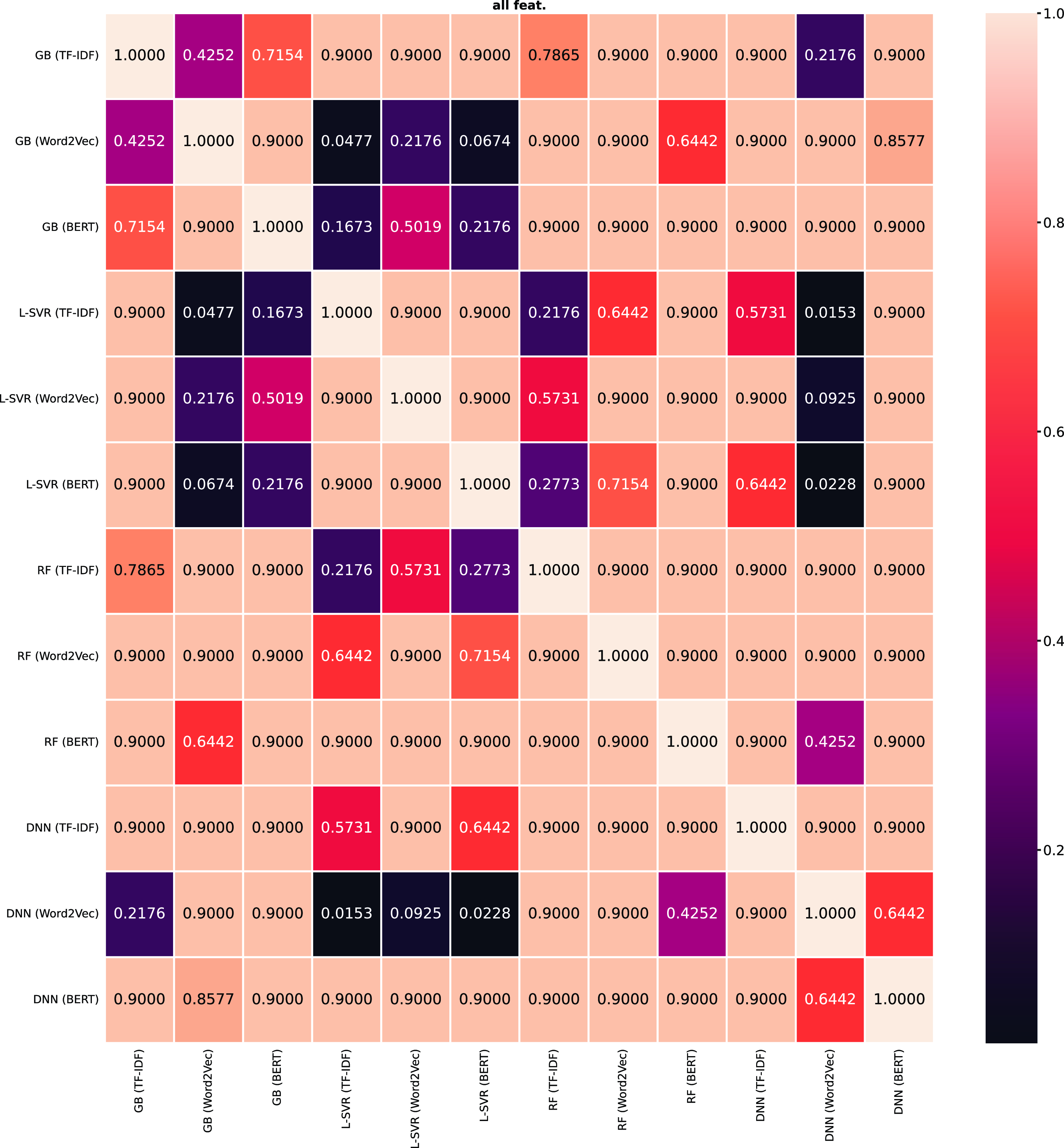
Figure A6. Nemenyi post hoc test of $\text{RMSE}$
scores for all features.
$\text{RMSE}$
scores for all features.


 Open access