


1. Introduction
The latest generation of masked language models (MLMs), which have demonstrated great success in practical applications, has also been the object of direct study (Belinkov et al., Reference Belinkov, Durrani, Dalvi, Sajjad and Glass2017a; Bisazza and Tump, Reference Bisazza and Tump2018; Conneau et al., Reference Conneau, Kruszewski, Lample, Barrault and Baroni2018a; Warstadt et al., Reference Warstadt, Cao, Grosu, Peng, Blix, Nie, Alsop, Bordia, Liu, Parrish, Wang, Phang, Mohananey, Htut, Jeretic and Bowman2019; Liu et al., Reference Liu, Gardner, Belinkov, Peters and Smith2019a; Tenney et al., Reference Tenney, Xia, Chen, Wang, Poliak, McCoy, Kim, Durme, Bowman, Das and Pavlick2019b; Ravichander, Belinkov, and Hovy, Reference Ravichander, Belinkov and Hovy2021; Belinkov, Reference Belinkov2022). To what extent do these models play the role of grammarians, rediscovering, and encoding linguistic structures like those found in theories of natural language syntax? In this paper, our focus is on morphology; since morphological systems vary greatly across languages, we turn to the multilingual variants of such models, exemplified by mBERT (Devlin et al., Reference Devlin, Chang, Lee and Toutanova2019) and XLM-RoBERTa (Conneau et al., Reference Conneau, Khandelwal, Goyal, Chaudhary, Wenzek, Guzmàn, Grave, Ott, Zettlemoyer and Stoyanov2020).
We first introduce a new morphological probing dataset of 247 probes, covering 42 languages from 10 families (Section 3) sampled from the Universal Dependencies (UD) Treebank (Nivre et al., Reference Nivre, de Marneffe, Ginter, Hajič, Manning, Pyysalo, Schuster, Tyers and Zeman2020).Footnote a As we argue in Section 2, this new dataset, which includes ambiguous word forms in context, enables substantially more extensive explorations than those considered in the past. To the best of our knowledge, this is the most extensive multilingual morphosyntactic probing dataset.
Our second contribution is an extensive probing study (Sections 4–8), focusing on mBERT and XLM-RoBERTa. We find that the features they learn are quite strong, outperforming an LSTM that treats sentences as sequences of characters, but which does not have the benefit of language model pre-training. Among other findings, we observe that XLM-RoBERTa’s larger vocabulary and embedding are better suited for a multilingual context than mBERT’s, and, extending the work of Zhang and Bowman (Reference Zhang and Bowman2018) on recurrent networks, Transformer-based MLMs may memorize word identities and their configurations in the training data. Our study includes several ablations (Section 8) designed to address potential shortcomings of probing studies raised by Belinkov (Reference Belinkov2022) and Ravichander et al. (Reference Ravichander, Belinkov and Hovy2021).
Finally, we aim to shed light not only on the models, but on how linguistic context cues morphological categorization. Specifically, where in the context does the information reside? Because our dataset offers a large number (247) of tasks, emergent patterns may correspond to general properties of language. Our first method (Section 6) perturbs probe task instances (both at training time and test time). Perturbations include masking the probe instance’s target word, words in the left and/or right context, and permuting the words in a sentence. Unsurprisingly, the target word itself is most important. We measure the effect on the probe’s accuracy and find that patterns of these effects across different perturbations tend to be similar within typological language groups.
The second method (Section 7) builds on the notion of perturbations and seeks to assign responsibility to different positions in the context of a word, using Shapley (Reference Shapley1951) values. We find a tendency across most tasks to rely more strongly on left context than on right context.Footnote b Given that there is no directional bias in Transformer-based models like mBERT and XLM-RoBERTa, this asymmetry—that morphological information appears to spread progressively—is quite surprising but significant.Footnote c Moreover, the few cases where it does not hold have straightforward linguistic explanations.
Though there are limitations to this study (e.g., the 42 languages we consider are dominated by Indo-European languages), we believe it exemplifies a new direction in corpus-based study of phenomena across languages, through the lens of language modeling, in combination with longstanding annotation and analysis methods (e.g., Shapley values). Remarkably, we can generally tie the exceptions to the dominant Shapley pattern to language-specific typological facts (see Section 7.3), which goes a long way toward explaining the reasonable (though imperfect) recovery (see Section 6) of the standard linguistic typology based on perturbation effects alone.
2. Related work and background
The observation that morphosyntactic features can simultaneously impact more than one word goes back to antiquity: Apollonius Dyscolus in the Greek and Pāṇini in the Indian tradition both explained the phenomenon by agreement rules that are typically not at all sensitive to linear order (Householder, Reference Householder1981; Kiparsky, Reference Kiparsky2009). This is especially clear for the Greek and Sanskrit cases, where the word order is sufficiently free for the trigger to come sometimes before, and sometimes after, the affected (target) word.Footnote d
The direction of control can be sensitive to the linking category as well (Deal, Reference Deal2015), but in this paper we will speak of directionality only in terms of temporal “before-after” order, using “left context” to mean words preceding the target and “right context” for words following it. Also, we use “target” only to mean the element probed, irrespective of whether it is controlling or controlled (a decision not always easy to make).
Qualitative micro-analysis of specific cases has been performed on many languages with diametrically different grammars (Lapointe, Reference Lapointe1990, Reference Lapointe1992; Brown, Reference Brown2001; Adelaar, Reference Adelaar2005; Anderson, Reference Anderson2005; Anderson et al., Reference Anderson, Brown, Gaby and Lecarme2006), but quantitative analyses supported by larger datasets are largely absent (Can et al., Reference Can, Aleçakır, Manandhar and Bozşahin2022). Even if so, the models in question are attention-free ones which are shown to be insufficient to deal with long-term dependencies (Li, Fu, and Ma, Reference Li, Fu and Ma2020).
Here we take advantage of the recent appearance of both data and models suitable for large-scale quantitative analysis of the directional spreading of morphosyntactic features. The data, coming from UD treebanks (see Section 3.2), have suitable per-token but contextual representations for full sentences or paragraphs.
The models take advantage of the recent shift from the standard, identity-based, categorical variable-like unary treatment of the words. This shift was, perhaps, the main factor contributing to the success of neural network-based language modeling. The internal representations of such models, often manifested in their hidden activations, proved to be a fruitful encoding (Bengio, Ducharme, and Vincent, Reference Bengio, Ducharme and Vincent2000). These word embeddings, as they came to be known, are low-dimensional numerical representations, typically real-valued vectors. Thanks to their ability to solve semantic and linguistic analogies both Word2Vec (Mikolov et al., Reference Mikolov, Chen, Corrado and Dean2013) and GloVe (Pennington, Socher, and Manning, Reference Pennington, Socher and Manning2014) gathered great interest. For a recent granular survey of progress toward pre-trained language models, see Qiu et al. (Reference Qiu, Sun, Xu, Shao, Dai and Huang2020) and Belinkov and Glass (Reference Belinkov and Glass2019), and for reviewing the literature on probing internal representations see Belinkov (Reference Belinkov2022).
2.1 Contextual language models
Contextual language models took the relevance of the context further in that they take a long sequence of words (even multiple sentences) as their input and assign a vector to each segment, typically a subword, so that the same word has distinct representations depending on its context. One of the first widely available contextual models was ELMo (Peters et al., Reference Peters, Neumann, Iyyer, Gardner, Clark, Lee and Zettlemoyer2018), which handled homonymy and polysemy much better than the context-independent embeddings, resulting in a significant performance increase on downstream NLP tasks when used in combination with other neural text classifiers (Peters et al., Reference Peters, Neumann, Iyyer, Gardner, Clark, Lee and Zettlemoyer2018; Qiu et al., Reference Qiu, Sun, Xu, Shao, Dai and Huang2020). Another major improvement in line was the introduction of Transformer-based (Vaswani et al., Reference Vaswani, Shazeer, Parmar, Uszkoreit, Jones, Gomez, Kaiser and Polosukhin2017) MLMs and their embeddings.
2.1.1 Multilingual BERT
BERT is a language model built on Transformer layers. Devlin et al. (Reference Devlin, Chang, Lee and Toutanova2019) introduced two BERT “sizes,” a base model and a large model. BERT-base has 12 Transformer layers with 12 attention heads. The hidden size of each layer is 768. BERT-large has 24 layers with 16 heads and 1024 hidden units. BERT-base has 110M/86M parameters with/without the embeddings; BERT-large has 340M/303M parameters with/without the embeddings. The size of the embedding depends on the size of the vocabulary which is specific to each pre-trained BERT model.
Multilingual BERT (mBERT) was released along with BERT, supporting 104 languages. The main difference is that mBERT is trained on text from many languages. In particular, it was trained on resource-balancedFootnote e Wikipedia dumps with a shared vocabulary across the supported languages. As a BERT-base model, its 12 Transformer layers have 86M parameters, while its large vocabulary requires an embedding with 92M additional parameters.Footnote f
2.1.2 XLM-RoBERTa
XLM-RoBERTa is a hybrid model mixing together features of two popular Transformer-based models, XLM (Conneau and Lample, Reference Conneau and Lample2019) and RoBERTa (Liu et al., Reference Liu, Ott, Goyal, Du, Joshi, Chen, Levy, Lewis, Zettlemoyer and Stoyanov2019b).
XLM is trained on both MLM and translation language modeling objective on parallel sentences. In contrast, XLM-RoBERTa is trained using the MLM objective only, like RoBERTa. The main difference between XLM-RoBERTa and RoBERTa remains the scale of the corpora they were trained on: XLM-RoBERTa’s multilingual training corpora counts five times more tokens and more than twice as many (278M with embeddings) parameters than RoBERTa’s 124M (Conneau et al., Reference Conneau, Khandelwal, Goyal, Chaudhary, Wenzek, Guzmàn, Grave, Ott, Zettlemoyer and Stoyanov2020). Another major difference between these two models is that XLM-RoBERTa is trained in self-supervised manner, while the parallel corpora for XLM is a supervised teaching signal. In the Cross-lingual Natural Language Interface (Conneau et al., Reference Conneau, Rinott, Lample, Williams, Bowman, Schwenk and Stoyanov2018b) evaluation of mBERT, XLM, and XLM-RoBERTa, the latter outperformed the other MLMs in all the languages tested by Conneau et al. (Reference Conneau, Khandelwal, Goyal, Chaudhary, Wenzek, Guzmàn, Grave, Ott, Zettlemoyer and Stoyanov2020).
2.1.3 Directionality
One of the Transformer architecture’s main novelties was the removal of recurrent connections, thereby discarding the ordering of the input symbols. Instead of recurrent connections, word order is expressed through positional encoding, a simple position-dependent value added to the subword embedding. Transformers have no inherent bias toward directionality. This means that our results on the asymmetrical nature of morphosyntax (c.f. Section 9) can only be attributed to the language, rather than the model.
2.1.4 Tokenization
The idea of an intermediate subword unit between character and word tokenization is common to mBERT and XLM-RoBERTa. The inventory of subwords is learned via simple frequency-based methods starting with byte pair encoding (BPE; Gage, Reference Gage1994). Initially, characters are added to the inventory, and BPE repeatedly merges the most frequent bigrams. This process ends when the inventory reaches a predefined size. The resulting subword inventory contains frequent character sequences, often full words, as well as the character alphabet as a fallback when longer sequences are not present in the input text. During inference time, the longest possible sequence is used starting from the beginning of the word. mBERT uses the WordPiece algorithm (Wu et al., Reference Wu, Schuster, Chen, Le, Norouzi, Macherey, Krikun, Cao, Gao, Macherey, Klingner, Shah, Johnson, Liu, Kaiser, Gouws, Kato, Kudo, Kazawa, Stevens, Kurian, Patil, Wang, Young, Smith, Riesa, Rudnick, Vinyals, Corrado, Hughes and Dean2016), a modification of BPE. XLM-RoBERTa uses the Sentence Piece algorithm (Kudo and Richardson, Reference Kudo and Richardson2018), another variant of BPE.
Each BERT model has its own vocabulary. The vocabulary is trained before the model, not in an end-to-end fashion like the rest of the model parameters. mBERT and XLM-RoBERTa both share the vocabulary across 100 languages with no distinction between the languages. This means that a subword may be used in multiple languages that share the same script. The subwords are differentiated whether they are word-initial or continuation symbols. mBERT marks the continuation symbols by prefixing them with ##. In contrast, XLM-RoBERTa marks the word-initial symbols rather than the continuation symbols, with a Unicode lower eighth block (2581). The idea is that both these marks are almost non-existent in natural text so it is easy to recover the original token boundaries.
mBERT uses a vocabulary with 118k subwords, while XLM-RoBERTa’s vocabulary has 250k subwords. This means that XLM-RoBERTa tends to generate fewer subwords for a given token, because longer partial matches are found more easily. Ács (Reference Ács2019) defines a tokenizer’s fertility as the proportion of subwords to tokens. The higher this number is, the more often the tokenizer splits a token. mBERT’s average fertility on our full probing dataset is 1.9, while XLM-RoBERTa’s fertility is 1.7. The target words that we probe have much higher fertility (3.1 for mBERT and 2.6 for XLM-RoBERTa). We attribute this to the fact that morphology is often expressed in affixes, making the word longer, and that longer words tend to have more morphological labels. Both tokenizers have the highest fertility in Belarusian (2.6 and 2.2) out of the 42 languages we consider in this paper. mBERT has the lowest fertility in English (1.7) and XLM-RoBERTa in Urdu (1.4).
2.2 Probing
Learning general-purpose language representations (embeddings) is a significant thread of the NLP research (Conneau and Kiela, Reference Conneau and Kiela2018). According to Devlin et al. (Reference Devlin, Chang, Lee and Toutanova2019), there are two major strategies to exploit the linguistic abilities of these internal representations of language models pre-trained either for neural machine translation (NMT) or language modeling in general. The feature-based approach, such as ELMo (Peters et al., Reference Peters, Neumann, Iyyer, Gardner, Clark, Lee and Zettlemoyer2018), uses dedicated model architectures for each downstream task, where pre-trained representations are included but remain unchanged. The fine-tuning approach, exemplified by GPT (Radford et al., Reference Radford, Narasimhan, Salimans and Sutskever2018), strives to modify all the LM’s parameters with as few new task-specific parameters as possible.
From this perspective, probing is a feature-based approach, with few new parameters. The goal of probing is not to enrich, but rather to explain the neural representations of the model. Probes use auxiliary classifiers (also called diagnostic classifiers) hooked to a pre-trained model that has frozen weights to train a minimal-architecture classifier—typically linear or an multilayer perceptron (MLP)—to predict a specific linguistic feature of the input. The performance of the classifier is considered indicative of the model’s “knowledge” in a particular task.
Probing as an explanation method was first used to evaluate static embeddings for part-of-speech and morphological features by Köhn (Reference Köhn2015) and Gupta et al. (Reference Gupta, Boleda, Baroni and Padó2015), paving the way for other studies to extend the body of research to semantic tasks (Shi, Padhi, and Knight, Reference Shi, Padhi and Knight2016; Ettinger, Elgohary, and Resnik, Reference Ettinger, Elgohary and Resnik2016; Veldhoen, Hupkes, and Zuidema, Reference Veldhoen, Hupkes and Zuidema2016; Qian, Qiu, and Huang, Reference Qian, Qiu and Huang2016; Adi et al., Reference Adi, Kermany, Belinkov, Lavi and Goldberg2017; Belinkov et al., Reference Belinkov, Màrquez, Sajjad, Durrani, Dalvi and Glass2017b; Conneau and Kiela, Reference Conneau and Kiela2018), syntax (Hewitt and Manning, Reference Hewitt and Manning2019; Goldberg, Reference Goldberg2019; Arps et al., Reference Arps, Samih, Kallmeyer and Sajjad2022), and multimodal tasks as well (Karpathy and Fei-Fei, Reference Karpathy and Fei-Fei2017; Kádár et al., Reference Kádár, Chrupala and Alishahi2017). With MLMs constantly improving the state of the art in most of the NLP benchmark tasks (Qiu et al., Reference Qiu, Sun, Xu, Shao, Dai and Huang2020), the embedding evaluation studies turned to probe these LMs (Conneau et al., Reference Conneau, Kruszewski, Lample, Barrault and Baroni2018a; Warstadt et al., Reference Warstadt, Cao, Grosu, Peng, Blix, Nie, Alsop, Bordia, Liu, Parrish, Wang, Phang, Mohananey, Htut, Jeretic and Bowman2019; Liu et al., Reference Liu, Gardner, Belinkov, Peters and Smith2019a; Tenney et al., Reference Tenney, Xia, Chen, Wang, Poliak, McCoy, Kim, Durme, Bowman, Das and Pavlick2019b) and contextual NMT models (Belinkov et al., Reference Belinkov, Durrani, Dalvi, Sajjad and Glass2017a; Bisazza and Tump, Reference Bisazza and Tump2018).
Although the analysis of NMT models provided many insights by comparing NMTs’ performance in probing tasks for multiple languages, the objective to compare the morphosyntactic features of multiple languages (Köhn, Reference Köhn2015) with the models trained on multilingual corpora. For a wider range of model architectures, mostly recurrent ones, see Conneau and Kiela (Reference Conneau and Kiela2018), Şahin et al. (Reference Şahin, Vania, Kuznetsov and Gurevych2020), and Edmiston (Reference Edmiston2020); for Transformer-based architectures, see Liu et al. (Reference Liu, Gardner, Belinkov, Peters and Smith2019a), Ravishankar et al. (Reference Ravishankar, Gökırmak, Øvrelid and Velldal2019), Reif et al. (Reference Reif, Yuan, Wattenberg, Viegas, Coenen, Pearce and Kim2019), Chi, Hewitt and Manning (Reference Chi, Hewitt and Manning2020), Mikhailov, Serikov and Artemova (Reference Mikhailov, Serikov and Artemova2021), and Shapiro, Paullada and Steinert-Threlkeld (Reference Shapiro, Paullada and Steinert-Threlkeld2021). Probing multilingual models (as opposed to NMT models) had the advantage of not requiring huge parallel corpora for training. As a result, most of the research community has turned to multilingual MLM probing in recent years (Ravishankar et al., Reference Ravishankar, Gökırmak, Øvrelid and Velldal2019; Şahin et al., Reference Şahin, Vania, Kuznetsov and Gurevych2020; Chi et al., Reference Chi, Hewitt and Manning2020; Mikhailov et al., Reference Mikhailov, Serikov and Artemova2021; Shapiro et al., Reference Shapiro, Paullada and Steinert-Threlkeld2021; Arps et al., Reference Arps, Samih, Kallmeyer and Sajjad2022). Our work adds morphology to this field of NLP engineering by:
-
• Extending the number of languages included in morphological probing to 42 languages.Footnote g
-
• Inclusion of ambiguous word forms Footnote h in the probing dataset in order to make the task more realistic. The MLMs we probe are capable of disambiguating such word forms based on the context.
-
• Inclusion of infrequent words as well, as opposed to Şahin et al. (Reference Şahin, Vania, Kuznetsov and Gurevych2020), whose study only considers frequent words.
-
• Novel ablations and probing controls (see Section 6).
-
• Bypassing auxiliary pseudo-tasks such as Character bin, Tag count, SameFeat, Oddfeat (Şahin et al., Reference Şahin, Vania, Kuznetsov and Gurevych2020). Such downstream tasks target proxies (artificial features, which are indicative of morphological ones) rather than the actual morphological features we concentrate on.
-
• Supporting our findings with in-depth analysis of the results by means of Shapley values.
3. Data
We define a probing task as a triple of $\langle$
language, POS, morphological feature
$\langle$
language, POS, morphological feature $\rangle$
, following UD’s naming conventions for morphological features (tags). Each sample is a sentence with a particular target word and a morphological feature value for it. For example, a sample from the task
$\rangle$
, following UD’s naming conventions for morphological features (tags). Each sample is a sentence with a particular target word and a morphological feature value for it. For example, a sample from the task $\langle$
English, VERB, Tense
$\langle$
English, VERB, Tense $\rangle$
, would look like “I read your letter yesterday,” where read is the target word and Past is the correct tag value.
$\rangle$
, would look like “I read your letter yesterday,” where read is the target word and Past is the correct tag value.
3.1 Choice of languages and tags
UD 2.9 (Nivre et al., Reference Nivre, de Marneffe, Ginter, Hajič, Manning, Pyysalo, Schuster, Tyers and Zeman2020) has treebanks in 122 languages. mBERT supports 104 languages while XLM-RoBERTa supports 100 languages. There are 55 languages in the intersection of these three sets. We include every language from this set except those where it is impossible to sample enough probing data. This was unfortunately the case for Chinese, Japanese, and Vietnamese due to the lack of data with morphosyntactic information and in Korean due to the different tagset used in the largest treebanks. 11 other languages have insufficient data for sampling. In contrast with for example Şahin et al. (Reference Şahin, Vania, Kuznetsov and Gurevych2020), who used UniMorph for morphological tasks, a type-level morphological dataset, UD allows studying morphology in context (often expressed through syntax). Moreover, we extended UD 2.9 with Kote et al. (Reference Kote, Biba, Kanerva, Rönnqvist and Ginter2019), an Albanian treebank and with a silver standard Hungarian dataset (Nemeskey, Reference Nemeskey2020). The resulting probing dataset includes 42 languages.
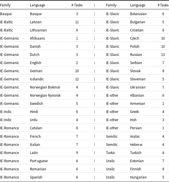
Table 1. List of languages and the number of tasks in each language.
UD has over 130 different morphosyntactic tags but most of them are only used for a couple of languages. In this work, we limit our analysis to four major tags that are available in most of the 42 languages: Case, Gender, Number, and Tense, and four open POS classes ADJ, NOUN, PROPN, and VERB. Out of the $4 \times 4 = 16$
POS-tag combinations, 14 are attested in our set of languages. The missing two,
$4 \times 4 = 16$
POS-tag combinations, 14 are attested in our set of languages. The missing two, $\langle$
NOUN, Tense
$\langle$
NOUN, Tense $\rangle$
and
$\rangle$
and $\langle$
PROPN, Tense
$\langle$
PROPN, Tense $\rangle$
, are linguistically implausible. One task,
$\rangle$
, are linguistically implausible. One task, $\langle$
ADJ, Tense
$\langle$
ADJ, Tense $\rangle$
, is only available in Estonian. The most common tasks are
$\rangle$
, is only available in Estonian. The most common tasks are $\langle$
NOUN, Number
$\langle$
NOUN, Number $\rangle$
,
$\rangle$
, $\langle$
NOUN, Gender
$\langle$
NOUN, Gender $\rangle$
, and
$\rangle$
, and $\langle$
VERB, Number
$\langle$
VERB, Number $\rangle$
, available in 37, 32, and 27 languages, respectively. 60% of the tasks are binary (e.g.,
$\rangle$
, available in 37, 32, and 27 languages, respectively. 60% of the tasks are binary (e.g., $\langle$
English, NOUN, Number
$\langle$
English, NOUN, Number $\rangle$
), 20.6% are three-way (e.g.,
$\rangle$
), 20.6% are three-way (e.g., $\langle$
German, NOUN, Gender
$\langle$
German, NOUN, Gender $\rangle$
) classification problems. The rest of the tasks have four or more classes.
$\rangle$
) classification problems. The rest of the tasks have four or more classes. $\langle$
Hungarian, NOUN, Case
$\langle$
Hungarian, NOUN, Case $\rangle$
has the most classes with 18 distinct noun cases, followed by
$\rangle$
has the most classes with 18 distinct noun cases, followed by $\langle$
Estonian, NOUN, Case
$\langle$
Estonian, NOUN, Case $\rangle$
,
$\rangle$
, $\langle$
Finnish, NOUN, Case
$\langle$
Finnish, NOUN, Case $\rangle$
, and
$\rangle$
, and $\langle$
Finnish, VERB, Case
$\langle$
Finnish, VERB, Case $\rangle$
with 15, 12, and 12 cases, respectively.
$\rangle$
with 15, 12, and 12 cases, respectively.
Table 1 lists the 42 languages included in the probing dataset. The task counts vary greatly. We only have one task in Afrikaans, Armenian, and Persian, while we sample 13 tasks in Russian and 12 in Icelandic.Footnote i The resulting dataset of 247 tasks is highly skewed toward European languages as evidenced by Figure 1. The Slavic family in particular accounts for almost one-third of the full dataset. This is due to two facts. First, Slavic languages have rich morphology so most POS-tag combinations exist in them (unlike, e.g., the Uralic languages which lack gender). Second, there are many Slavic languages, and their treebanks are very large, the Czech treebanks are over 2M tokens, while the Russian treebanks have 1.8M tokens. The modest number of non-European tasks is an important limitation of our study. Fortunately, the Indo-European language family is large and diverse enough that we have examples for many different morphosyntactic phenomena.
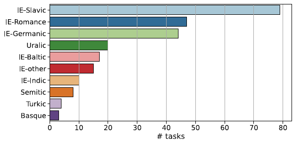
Figure 1. Number of tasks by language family.
3.2 Data generation
UD treebanks use the CoNLL-U format, where one line corresponds to one token and the token descriptors are separated by tabs. One such descriptor is the morphosyntactic analysis of the token where the standard format looks like this: MorphoTag1=Value1—MophoTag2=Value2. This field may be empty but in practice most non-punctuation tokens have multiple morphosyntactic tags. Some treebanks do not include morphosyntactic tags or they use a different tagset; we excluded these. To generate the probing tasks, we use all data available in sufficient quantity with UD tags.
We merge treebanks in the same language but keep the train/development/test splits and use them to sample our train, development, and test sets until we obtain 2000 training, 200 development, and 200 test samples so that there is no overlap between the target words in the resulting sets. We exclude languages with fewer than 500 sentences. We limit sentence length to be between 3 and 40 tokens in the gold standard tokenization of UD. Of the candidate triples that remain, we generate tasks where class imbalance is limited to 3:1. We attain this by two operations: by downsampling large classes and by discarding small classes that occur fewer than 200 times in all UD treebanks in a particular language.Footnote j We discard tasks where these sample counts are impossible to attain with our constraints. This leaves 247 tasks across 42 languages from 10 language families. Additional statistics are included in Appendix A.
4. Methods
In principle, both mBERT and XLM-RoBERTa are trainable, but the number of parameters is large (178M and 278M, respectively), and morphologically tagged data are simply not available in quantities that would make this feasible. We therefore keep the models fixed and train only a small auxiliary classifier, a MLP, typically with a single hidden layer and 50 neurons (for variations see Section 8.1) that operates on the weighted sum of the vectors returned by each layer of the large model that is being probed. This setup is depicted for mBERT in Figure 2.
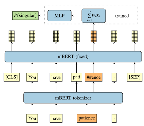
Figure 2. Probing architecture. Input is tokenized into wordpieces, and a weighted sum of the mBERT layers taken on the last wordpiece of the target word is used for classification by an MLP. Only the MLP parameters and the layer weights $w_i$
are trained.
$w_i$
are trained. $\mathbf{x}_i$
is the output vector of the
$\mathbf{x}_i$
is the output vector of the $i$
th layer,
$i$
th layer, $w_i$
is the learned layer weight. The example task here is
$w_i$
is the learned layer weight. The example task here is $\langle$
English, NOUN, Number
$\langle$
English, NOUN, Number $\rangle$
.
$\rangle$
.
Probing as a methodology for learning about representations has had its share of criticism (Ravichander et al., Reference Ravichander, Belinkov and Hovy2021; Belinkov, Reference Belinkov2022). In particular, Belinkov (Reference Belinkov2022) argues that probing classifiers often tell us more about the classifier itself or the dataset than the probed model. We run several controls and show that our results are more robust. In particular, the probing accuracy is largely independent of the classifier hyperparameters, linear probes are similar to non-linear probes (see Section 8.1); layer effects are consistent with other probes (see Section 8.2); fine-tuning the models is time intensive and the results are significantly worse (see Section 8.3); and the probes work significantly better on pre-trained checkpoints than on randomly initialized BERT models (see Section 8.4).
4.1 Baselines
Our main baseline is chLSTM, a bidirectional characterFootnote k LSTM over the probing sentence. The input character sequence (including spaces) is passed through an embedding that maps each character to a 30 dimensional continuous vector. This vector is passed along to a one-layered LSTM with 100 hidden units. We extract the output corresponding to the first or the last character (see Section 4.3) and pass it to an MLP with one hidden layer with 50 neurons (identical to the MLM probing setup). The embedding, the LSTM, and the MLP are randomly initialized and trained end-to-end on the probing data alone. The parameter count is close to the MLM auxiliary classifiers’ parameter count (40k). Our motivation for this model can be summarized as:
-
• it is contextual;
-
• it is only trained on the probing data and we can assume that if a MLM performs better than chLSTM, it is probably due to the MLM’s pre-training, especially as the SIGMORPHON shared tasks are dominated by LSTM models;
-
• LSTMs are good at morphological inflection (Kann and Schütze, Reference Kann and Schütze2016; Cotterell et al., Reference Cotterell, Kirov, Sylak-Glassman, Walther, Vylomova, Xia, Faruqui, Kübler, Yarowsky, Eisner and Hulden2017), a related but more difficult task than morphosyntactic classification;
-
• it is a different model family than the Transformer-based MLMs, so any similarity in behavior, particularly our findings using Shapley values explored in Section 7, is likely due to linguistic reasons rather than some modeling bias.
Our secondary baseline is fastText (Bojanowski et al., Reference Bojanowski, Grave, Joulin and Mikolov2017), a multilingual word embedding trained on bags of character n-grams. We use the same type of MLP on top of fastText vectors. FastText is pre-trained, though less extensively than the MLMs.
Finally, we also run Stanza,Footnote l a high-quality NLP toolchain for many languages. Although there are undoubtedly better language-specific tools than Stanza for certain languages, it is outside the scope of this paper to find the best morphosyntactic tagger for 42 languages. The details of our Stanza setup are listed in Appendix B.
4.2 Experimental setup
All experiments including the baselines are trained using the Adam optimizer (Kingma and Ba, Reference Kingma and Ba2015) with $\text{lr}=0.001, \beta _1=0.9, \beta _2=0.999$
. We use early stopping based on development loss and accuracy. We use a 0.2 dropout between the input and hidden layer of the MLP and between the hidden and the output layers. The batch size is always set to 128 except in the fine-tuning experiments where it is set to 8. All results throughout the paper are averaged over 10 runs with different random seeds except the ones presented in Section 7 since they require an exponentially large number of experiments.
$\text{lr}=0.001, \beta _1=0.9, \beta _2=0.999$
. We use early stopping based on development loss and accuracy. We use a 0.2 dropout between the input and hidden layer of the MLP and between the hidden and the output layers. The batch size is always set to 128 except in the fine-tuning experiments where it is set to 8. All results throughout the paper are averaged over 10 runs with different random seeds except the ones presented in Section 7 since they require an exponentially large number of experiments.
4.3 Subword pooling
FastText maps every word to a single vector and can generate vectors for OOV words with an offline script. On the other hand, mBERT and chLSTM may assign multiple vectors to the target word. mBERT assigns a vector to each subword and chLSTM assigns a vector to each character. These models require a way to pool multiple vectors that correspond to the target word. Devlin et al. (Reference Devlin, Chang, Lee and Toutanova2019) used the first wordpiece of every token for named entity recognition. kondratyuk and straka (Reference Kondratyuk and Straka2019) and Kitaev et al. (Reference Kitaev, Cao and Klein2019) found no difference between using first, last, or max pooling for dependency parsing and constituency parsing in many languages. Ács et al. (Reference Ács, Kádár and Kornai2021) showed that the last subword is usually the best for morphology and more sophisticated pooling choices do not improve the results, so we only compare the first and the last subword for both mBERT and XLM-RoBERTa and use the better choice based on development accuracy. This turns out to be the last subword for 98% of the tasks. Similarly, we consider the first and the last character for chLSTM. The last character is the better choice in 82% of the tasks.
5. Results
5.1 Morphology in pre-trained language models
We first examine how well morphology can be recovered from the model representations. Table 2 shows the average probing accuracy on each morphological task. The average is computed over all languages each task is available in. XLM-RoBERTa is slightly better than mBERT, and both are clearly superior to chLSTM and fastText. The baselines are also close to each other but chLSTM is 0.6% better than fastText. Out of the 14 $\langle$
POS, tag
$\langle$
POS, tag $\rangle$
combinations, mBERT is only better than XLM-RoBERTa in
$\rangle$
combinations, mBERT is only better than XLM-RoBERTa in $\langle$
ADJ, Gender
$\langle$
ADJ, Gender $\rangle$
but the difference is not statistically significant (
$\rangle$
but the difference is not statistically significant ( $p\gt 0.05$
with Bonferroni correction).Footnote m In fact, XLM-RoBERTa is only statistically significantly better than mBERT at 5 POS-tag combinations out of the 14:
$p\gt 0.05$
with Bonferroni correction).Footnote m In fact, XLM-RoBERTa is only statistically significantly better than mBERT at 5 POS-tag combinations out of the 14: $\langle$
ADJ, Case
$\langle$
ADJ, Case $\rangle$
,
$\rangle$
, $\langle$
NOUN, Case
$\langle$
NOUN, Case $\rangle$
,
$\rangle$
, $\langle$
NOUN, Number
$\langle$
NOUN, Number $\rangle$
,
$\rangle$
, $\langle$
VERB, Number
$\langle$
VERB, Number $\rangle$
, and
$\rangle$
, and $\langle$
VERB, Tense
$\langle$
VERB, Tense $\rangle$
. Since chLSTM is the better baseline and it is a practical estimation of the maximum performance achievable with the probing data alone, we limit our analysis to chLSTM and the two MLMs.
$\rangle$
. Since chLSTM is the better baseline and it is a practical estimation of the maximum performance achievable with the probing data alone, we limit our analysis to chLSTM and the two MLMs.
Table 2. Average test accuracy over all languages by task and model
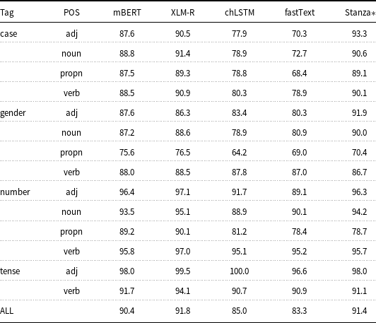
The last row is the average of all 247 tasks. Stanza does not support Albanian, so the six Albanian tasks are not included in the Stanza results.
Perhaps the most salient fact about these results is that the MLM-based systems perform in the high 80–90% level (only one task, $\langle$
PROPN, Gender
$\langle$
PROPN, Gender $\rangle$
is at 76%), something quite remarkable compared to the state of the art only a decade ago (Kurimo et al., Reference Kurimo, Virpioja, Turunen and Lagus2010). In fact, those current models that are tuned to individual tasks and languages can often go beyond the performance of the generic models presented here, but our interest is with universal morphological claims one can distill from adapting generic MLM models to highly language-specific tasks.Footnote n The auxiliary classifier has relatively few (40k) parameters, no more than the fully task-specifically trained baselines, nevertheless outperforms both chLSTM and fastText. This indicates clearly that the morphological knowledge is not in the auxiliary classifier alone, some of it must already be present in the pre-trained weights that come with mBERT and XLM-RoBERTa. For detailed comparison with randomized baselines, see Section 8.
$\rangle$
is at 76%), something quite remarkable compared to the state of the art only a decade ago (Kurimo et al., Reference Kurimo, Virpioja, Turunen and Lagus2010). In fact, those current models that are tuned to individual tasks and languages can often go beyond the performance of the generic models presented here, but our interest is with universal morphological claims one can distill from adapting generic MLM models to highly language-specific tasks.Footnote n The auxiliary classifier has relatively few (40k) parameters, no more than the fully task-specifically trained baselines, nevertheless outperforms both chLSTM and fastText. This indicates clearly that the morphological knowledge is not in the auxiliary classifier alone, some of it must already be present in the pre-trained weights that come with mBERT and XLM-RoBERTa. For detailed comparison with randomized baselines, see Section 8.
Figures 3 and 4 show the difference between the accuracy of the MLMs and chLSTM averaged over language families. chLSTM is only better than one or both of the pre-trained models in 8 tasks out of the 247, and the difference is never large.
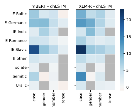
Figure 3. Difference in accuracy between mBERT (left) and chLSTM, and XLM-RoBERTa (right) and chLSTM grouped by language family and morphological category. Gray cells represent missing tasks.
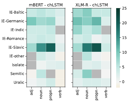
Figure 4. Difference in accuracy between mBERT (left) and chLSTM, and XLM-RoBERTa (right) and chLSTM grouped by language family and POS. Gray cells represent missing tasks.
We find a large number of tasks at the other end of the scale. Particularly, Slavic case and gender probes work much better in both mBERT and XLM-RoBERTa than in chLSTM. Slavic languages have highly complex declension with three genders, six to eight cases, and frequent syncretism. This explains why chLSTM is struggling to pick up the pattern from 2000 training samples alone. mBERT and XLM-RoBERTa were both trained on large datasets in each language and therefore may have picked up a general representation of gender and case.Footnote o It is also worth mentioning that among the 100 languages that these models support, Slavic languages are one of the largest language families with 10 or more languages. Figure 5 shows the differences for each Slavic language and task. The similarities appear more areal (Ukrainian and Belarus, Czech and Polish) than historical, though the major division into Eastern, Western, and Southern Slavic is still somewhat perceptible.
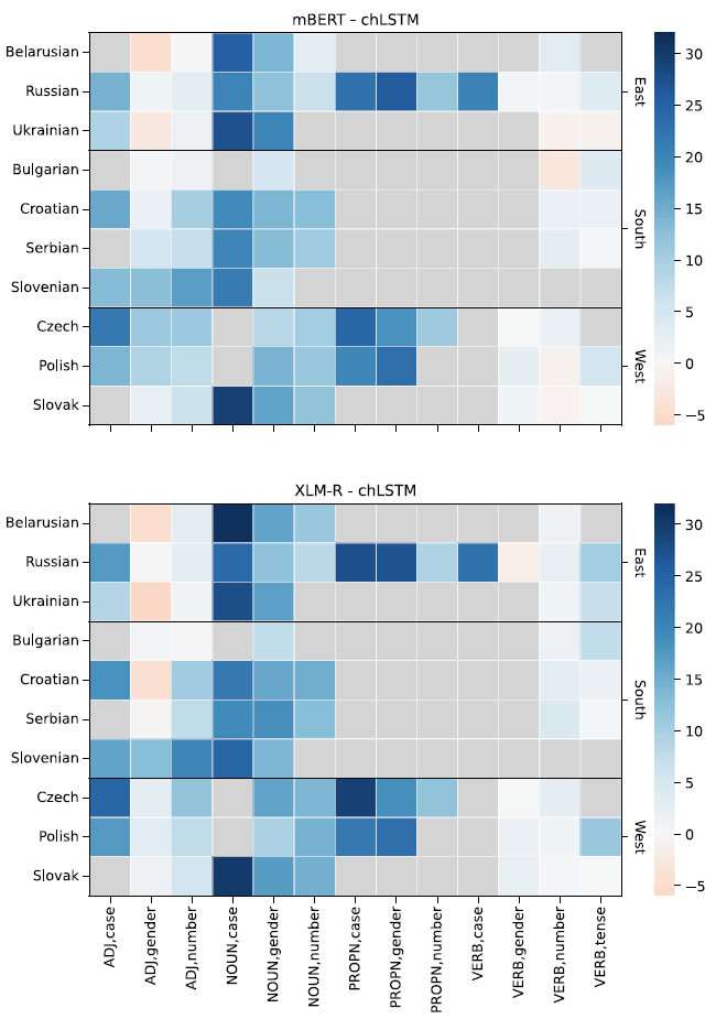
Figure 5. Task-by-task difference between the MLMs and chLSTM in Slavic languages. Gray cells represent missing tasks.
5.2 Comparison between mBERT and XLM-RoBERTa
Table 2 showed that XLM-RoBERTa is slightly better than mBERT on average and in every POS-tag category except $\langle$
ADJ, Gender
$\langle$
ADJ, Gender $\rangle$
. However, this advantage is not uniform over tag and POS as evidenced by Figure 6, which shows the number of tasks where one model is significantly better than the other. XLM-RoBERTa is always better or no worse than mBERT at case and tense tasks with the exception of
$\rangle$
. However, this advantage is not uniform over tag and POS as evidenced by Figure 6, which shows the number of tasks where one model is significantly better than the other. XLM-RoBERTa is always better or no worse than mBERT at case and tense tasks with the exception of $\langle$
Swedish, NOUN, Case
$\langle$
Swedish, NOUN, Case $\rangle$
and
$\rangle$
and $\langle$
Romanian, VERB, Tense
$\langle$
Romanian, VERB, Tense $\rangle$
, where mBERT is the stronger model.
$\rangle$
, where mBERT is the stronger model.
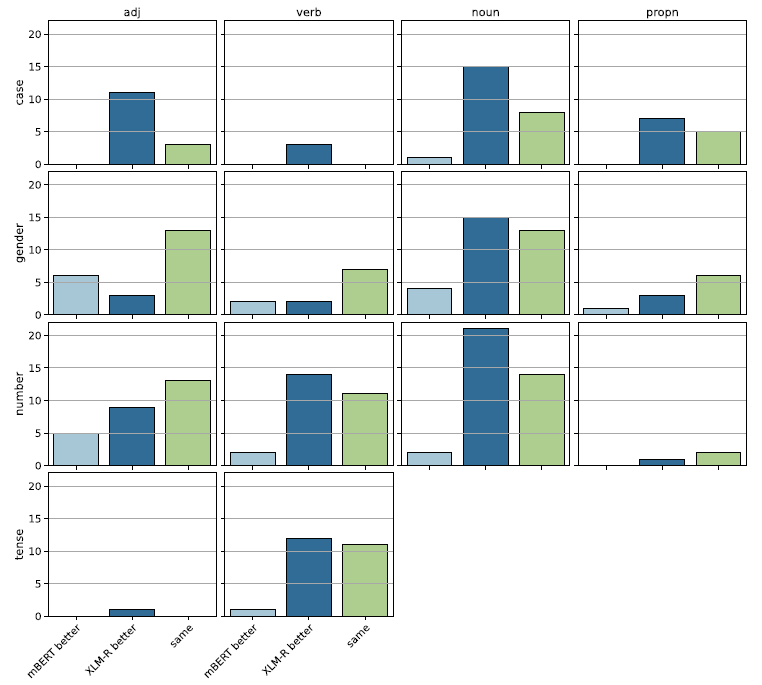
Figure 6. mBERT XLM-RoBERTa comparison by tag and by POS.
Figure 7 illustrates the same task counts by language family. We observe the same performance in most tasks from the Germanic and Romance language families. XLM-RoBERTa is better at the majority of the tasks from the Semitic, Slavic, and Uralic families, and the rest are more even. Interestingly, the two members of the Indic family in our dataset, Hindi and Urdu, behave differently. XLM-RoBERTa is better at five out of six Hindi tasks and the models are the same at the sixth task. mBERT, on the other hand, is better at one Urdu task and the models are the same at other three Urdu tasks. This might be due to the subtle differences in mBERT and XLM-RoBERTa subword tokenization introduced in 2.1.4.
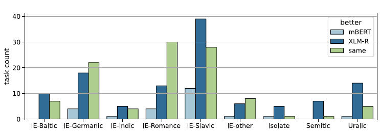
Figure 7. mBERT XLM-RoBERTa comparison by language family.
5.3 Difficult tasks
Some morphosyntactic tags are hard to retrieve from the model representations. In this section, we examine such tags and the results in more detail. Table 3 lists the 10 hardest tasks measured by the average accuracy of mBERT and XLM-RoBERTa. $\langle$
German, PROPN, Case
$\langle$
German, PROPN, Case $\rangle$
is difficult for two reasons. First, nouns are not inflected in German;Footnote p case is marked in the article of the noun. The article depends on both the case and the gender, and syncretism (ambiguity) is very high. This is reflected in the modest results for
$\rangle$
is difficult for two reasons. First, nouns are not inflected in German;Footnote p case is marked in the article of the noun. The article depends on both the case and the gender, and syncretism (ambiguity) is very high. This is reflected in the modest results for $\langle$
German, NOUN, Case
$\langle$
German, NOUN, Case $\rangle$
as well (72.9% for mBERT, 80.7% for XLM-RoBERTa). Second, proper nouns are often multiword expressions. Since all tokens of a multiword proper noun are tagged PROPN in UD, our sampling method may pick any of those tokens as a target token of a probing task.
$\rangle$
as well (72.9% for mBERT, 80.7% for XLM-RoBERTa). Second, proper nouns are often multiword expressions. Since all tokens of a multiword proper noun are tagged PROPN in UD, our sampling method may pick any of those tokens as a target token of a probing task.
Table 3. 10 hardest tasks.
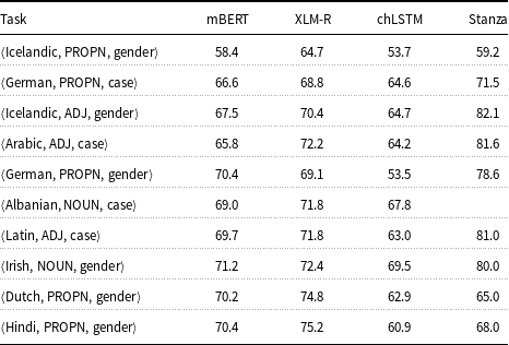
Another outlier is $\langle$
Arabic, ADJ, Case
$\langle$
Arabic, ADJ, Case $\rangle$
. Arabic adjectives usually follow the noun they agree with in case. There is no agreement with the elative case, and sometimes, the adjective precedes the noun which is in genitive, but the adjective is not. This kind of exceptionality may simply be too much to learn based on relatively few examples—it is still fair to say that grammarians (humans) are better pattern recognizers than MLMs.
$\rangle$
. Arabic adjectives usually follow the noun they agree with in case. There is no agreement with the elative case, and sometimes, the adjective precedes the noun which is in genitive, but the adjective is not. This kind of exceptionality may simply be too much to learn based on relatively few examples—it is still fair to say that grammarians (humans) are better pattern recognizers than MLMs.
6. Perturbations
In Section 6.1, we analyze the MLMs’ knowledge of morphology in more detail through a set of perturbations that remove some source of information from the probing sentence. We compare the different perturbations to the unperturbed MLMs, but observe that perturbation often reduces performance to the level of the contextual baseline (chLSTM) or even below. The effect of major perturbations is unmistakable. Table 4 exemplifies each perturbation.
Table 4. List of perturbation methods with examples.
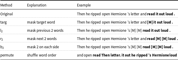
The target word is in bold. The mask symbol is abbreviated as [M].
Target masking
Languages with rich inflectional morphology tend to encode most, if not all, morphological information in the word form alone. We test this by hiding the word form, while keeping the rest of the sentence intact. Recall that BERT is trained with a cloze-style language modeling objective, that is 15% of tokens are replaced with a [MASK] token and the goal is to predict these. We employ this mask token to hide the target word (targ) from the auxiliary classifier. This means that all orthographic cues present in the word form are removed.Footnote q
Context masking
Many languages encode morphology in short phrases that span a few words, for example person/number agreement features on a verb that is immediately preceded by a subject. The verb tense of read, while ambiguous on its own, can often be disambiguated by looking at a few surrounding words, such as the presence of an auxiliary (didn’t), or a temporal expression. We use the relative position of a token to the target word, left context refers to the part of the sentence before the target word, while right context refers to the part after it. We try masking the left (l $_N$
), the right (r
$_N$
), the right (r $_N$
), and both sides (b
$_N$
), and both sides (b $_N$
), where
$_N$
), where $N$
refers to the number of masked tokens. We expand this analysis using Shapley values in Section 7.
$N$
refers to the number of masked tokens. We expand this analysis using Shapley values in Section 7.
Permute
Many languages have strict constraints on the order of words. A prime example is English, where little morphology is present at the word level, but reordering the words can change the meaning of a sentence dramatically. Consider the examples Mary loves John versus John loves Mary: in languages with case inflection, the distinction is made by the cases rather than the word order. It has been shown (Ettinger, Reference Ettinger2020; Sinha et al., Reference Sinha, Parthasarathi, Pineau and Williams2021) that BERT models are sensitive to word order in a variety of English and Mandarin tasks. We quantify the importance of word order by shuffling the words in the sentence.
6.1 Results
Perturbations change the input sequence or the probing setup in a way that removes information and should result in a decrease in probing accuracy. Given the large number of tasks and multiple perturbations, instead of listing all individual data points, we average the results over POS, tags, and language families and point out the main trends and outliers. The overall average perturbation results are listed in Table 5.

Our main group of perturbations involves masking one or more words in the input sentence. Both models have dedicated mask symbols, which we use to replace certain input words. In particular, targ masks the target word, where most of the information is contained—precisely how much will be discussed in Section 7. Permute shuffles the entire context, leaving the target word fixed, l $_{2}$
masks the two words preceding that target word, r
$_{2}$
masks the two words preceding that target word, r $_{2}$
masks the two words following the target and b
$_{2}$
masks the two words following the target and b $_{2}$
masks both the preceding two and the following two words. Remarkably, permute and b
$_{2}$
masks both the preceding two and the following two words. Remarkably, permute and b $_{2}$
are highly correlated, a matter we shall return to in 6.1.2. Figure 8 shows the average test accuracy of the probes by perturbation grouped by POS.
$_{2}$
are highly correlated, a matter we shall return to in 6.1.2. Figure 8 shows the average test accuracy of the probes by perturbation grouped by POS.
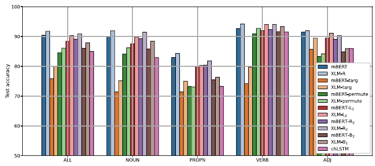
Figure 8. Test accuracy of the perturbed probes grouped by POS. The first group is the average of all 247 tasks. The first two bars in each group are the unperturbed probes’ accuracy.
Since the net changes caused by masking are often quite small, particularly for verbs, we define the effect of perturbation $p$
on task
$p$
on task $t$
when probing model
$t$
when probing model $m$
as:
$m$
as:
 \begin{equation} E(m, t, p) = 1 - \frac{\text{Acc}(m, t, p)}{\text{Acc}(m, t)}, \end{equation}
where $\text{Acc}(m, t)$
is the unperturbed probing accuracy on task
$\text{Acc}(m, t)$
is the unperturbed probing accuracy on task $t$
by model
$t$
by model $m$
. We present the effect values as percentages of the original accuracy. 50% effect means that the probing accuracy is reduced by half. Negative effect means that the probing accuracy improves due to a perturbation.
$m$
. We present the effect values as percentages of the original accuracy. 50% effect means that the probing accuracy is reduced by half. Negative effect means that the probing accuracy improves due to a perturbation.
6.1.1 Context masking
Proper nouns seem to be affected the most by context masking perturbations. This is probably caused by the lack of morphological information in the word form itself, at least in Slavic languages, where proper nouns are often indeclinable. The models pick up much of the information from the context. We shall examine this in more detail in Section 7.
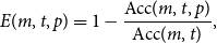
Although the average effect is rather modest, there are some tasks that are affected significantly by context masking perturbations. Figure 9 shows the effect (as defined in Equation 1) by tag.
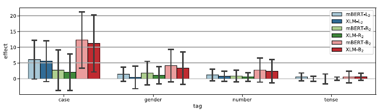
Figure 9. The effect of context masking perturbations by tag. Error bars indicate the standard deviation.
Since case is affected the most, we examine it a little closer. Figure 10 shows the effect of context masking on case tasks grouped by language family. Uralic results are barely affected by context masking, which confirms that the target word alone is indicative of the case in Uralic languages. Germanic, Semitic, and Slavic case probes are moderately affected by l $_{2}$
, and somewhat surprisingly, we find a small improvement in probing accuracy, by r
$_{2}$
, and somewhat surprisingly, we find a small improvement in probing accuracy, by r $_{2}$
. Indic probes are the opposite, r
$_{2}$
. Indic probes are the opposite, r $_{2}$
has over 20% effect, while l
$_{2}$
has over 20% effect, while l $_{2}$
is close to 0. Indic word order is quite complex, with a basic SOV word order affected both by split ergativity and communicative dynamism (topic/focus) effects (Jawaid and Zeman, Reference Jawaid and Zeman2011). Again, we suspect that these complexities overwhelm the MLMs, which work best with mountains of data, typically multi-gigaword corpora, three to four orders of magnitude more than what can reasonably be expected from primary linguistic data, less than thirty million words during language acquisition (Hart and Risley, Reference Hart and Risley1995).
$_{2}$
is close to 0. Indic word order is quite complex, with a basic SOV word order affected both by split ergativity and communicative dynamism (topic/focus) effects (Jawaid and Zeman, Reference Jawaid and Zeman2011). Again, we suspect that these complexities overwhelm the MLMs, which work best with mountains of data, typically multi-gigaword corpora, three to four orders of magnitude more than what can reasonably be expected from primary linguistic data, less than thirty million words during language acquisition (Hart and Risley, Reference Hart and Risley1995).
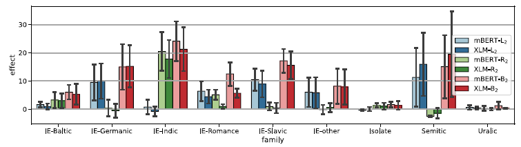
Figure 10. The effect of context masking on case tasks grouped by language family. Error bars indicate the standard deviation.
6.1.2 Target masking and word order
We discuss targ and permute in conjunction since they often have inverse effect for certain languages and language families. Target masking or targ is by far the most destructive perturbation with an average effect of 16.1% for mBERT and 12.7% for XLM-RoBERTa. Permute is also a significant perturbation, particularly for case tasks and adjectives. As Figure 11 shows, the effects differ widely among tasks but some trends are clearly visible. targ clearly plays an important role in many if not all tasks. Verbal tasks rely almost exclusively on the target form and permute has little to no effect. Verbal morphology is most often marked on the verb form itself, so this not surprising. Nouns and proper nouns behave similarly with the exception of case tasks. Case tasks show a mixed picture for all four parts of speech. targ and permute both have a moderate effect. This might be explained by the fact that case is expressed in two distinct ways depending on the language. Agglutinative languages express case through suffixes, while analytic languages, such as English, express case with prepositions. In other words, the context is unnecessary for the first group and indispensable for the second.

Figure 11. The effect of targ and permute. Error bars indicate the standard deviation.
Both targ and permute are markedly small for gender and number tasks in adjectives. This is likely due to the fact that adjectives do not determine the gender or the number of the nominal head but rather copy (agree with) it.
Figure 12 shows the effect of targ and permute by language family. Although the standard deviations are often larger than the mean effects, the trends are clear for multiple language families. The Uralic family is barely affected by permute while targ has over 20% effect for both models. Targ has a larger effect than permute for the Baltic and the Romance family and isolate languages. Indic tasks on the other hand tend to have little change due to targ, while permute has the largest effect for this family.
Figure 12. The effect of targ and permute by language family. Error bars indicate the standard deviation.
6.1.3 Relationship between perturbations
In the previous section, we showed that targ and permute often have an inverse correlation. Here we quantify their relationship as well as the relationship between all perturbations across the two models. First, we show that the effects across models are highly correlated as evidenced by Figure 13, which shows the pairwise Pearson’s correlation of the effects of each perturbation pair. The matrix is almost symmetrical. The main diagonal is close to one, which means that the same perturbation affects the two models in a very similar way. This suggests not just that the models are quite similar (see also Figure 14 depicting the correlation between perturbations in each model side by side) but also that the perturbations tell us more about morphology than about the models themselves.
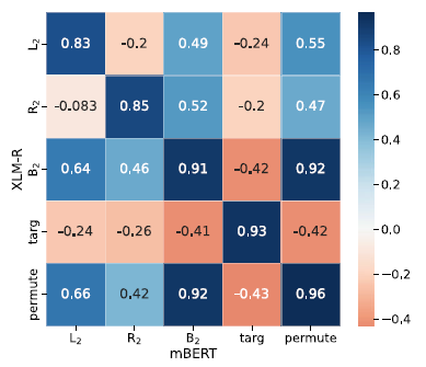
Figure 13. The pairwise Pearson correlation of perturbation effects between the two models.
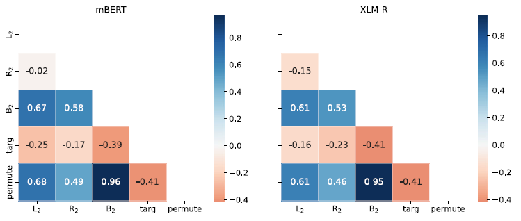
Figure 14. The pairwise Pearson correlation of perturbation effects by model.
6.2 Typology
While our dataset is too small for drawing far-reaching conclusions, we are beginning to see an emerging typological pattern in the effects of perturbation as defined in Equation (1). We cluster the languages by the effects of the perturbations on each task. There are five perturbations and 14 tasks, available as input features for the clustering algorithm, but many are missing in most languages. We use the column averages as imputation values. Since a single clustering run shows highly unstable results, we aggregate over 100 runs of $K$
-means clustering with
$K$
-means clustering with $K$
drawn uniformly between three and eight clusters. We then count how many times each pair of languages were clustered into the same cluster. Figure 15 illustrates the co-occurrence counts for XLM-RoBERTa. Since mBERT results are very similar, we limit our analysis to XLM-RoBERTa for simplicity.
$K$
drawn uniformly between three and eight clusters. We then count how many times each pair of languages were clustered into the same cluster. Figure 15 illustrates the co-occurrence counts for XLM-RoBERTa. Since mBERT results are very similar, we limit our analysis to XLM-RoBERTa for simplicity.
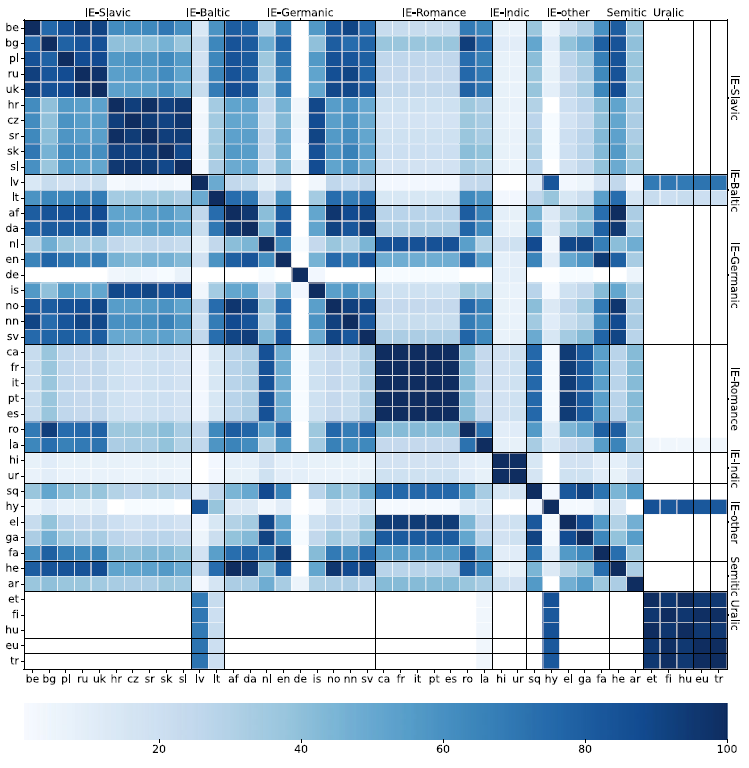
Figure 15. Co-occurrence counts for each language pair over 100 clustering runs. Languages are sorted by family and a line is added between families.
Language families tend to be clustered together with some notable exceptions. German is seldom clustered together with other languages, including other members of the Germanic family, except perhaps for Icelandic. To a lesser extent, Latin is an outlier in the Romance family—it clusters better with Romanian than with Western or Southern Romance. The two Indic languages are almost always in a single cluster without any other languages, but the two Semitic languages are almost never in the same cluster. Arabic tends to be in its own cluster, while Hebrew is often grouped with Indo-European languages. The Uralic family forms a strong cluster along with Basque and Turkish. These languages have highly complex agglutination and they all lack gender, so this is not surprising.
7. Shapley values
Having measured the (generally harmful) effect of perturbations, our next goal is to assign responsibility (blame) to the contributing factors. We use Shapley values for this purpose. For a general introduction, see Shapley (Reference Shapley1951) and Lundberg and Lee (Reference Lundberg and Lee2017); for motivation of Shapley values in NLP, see Ethayarajh and Jurafsky (Reference Ethayarajh and Jurafsky2021). We consider a probe as a coalition game of the words of the sentence. We treat each token position as a player in the game. The tokens are defined by their relative position to the target token. A sentence is a sequence defined as $ L_k, L_{k-1}, \dots, L_1, T, R_1, R_2, \dots, R_{m}$
, where
$ L_k, L_{k-1}, \dots, L_1, T, R_1, R_2, \dots, R_{m}$
, where $k$
is the number of words that precede that target word and
$k$
is the number of words that precede that target word and $m$
is the number of words that follow it. The tokens far to the left are considered as belonging to a single position (
$m$
is the number of words that follow it. The tokens far to the left are considered as belonging to a single position ( $-4^-$
), those far to the right to another position (
$-4^-$
), those far to the right to another position ( $4^+$
), so we have a total of nine players
$4^+$
), so we have a total of nine players $N=\{-4^-,-3,-2,-1,0,1,2,3,4^+\}$
. On a given task, we can remove the contribution of a player
$N=\{-4^-,-3,-2,-1,0,1,2,3,4^+\}$
. On a given task, we can remove the contribution of a player $i$
by masking the word(s) in positions corresponding to that player. The Shapley value
$i$
by masking the word(s) in positions corresponding to that player. The Shapley value $\varphi (i)$
corresponding to this player is computed as
$\varphi (i)$
corresponding to this player is computed as
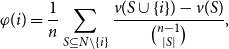 \begin{equation} \varphi (i) = \frac{1}{n} \sum _{S \subseteq N \setminus \{i\}} \frac{v(S \cup \{i\}) - v(S)}{\binom{n-1}{|S|}}, \end{equation}
where $n$
is the total number of players, 9 in our case, and
$n$
is the total number of players, 9 in our case, and $v(S)$
is the value of coalition
$v(S)$
is the value of coalition $S$
(a set of players, here positions) on the given tasks.
$S$
(a set of players, here positions) on the given tasks. $v(S)$
is a function of the accuracies (
$v(S)$
is a function of the accuracies ( $\mathrm{Acc}$
) of the task’s probe with coalition
$\mathrm{Acc}$
) of the task’s probe with coalition $S$
, the full set of players
$S$
, the full set of players $N$
, and the model. When all players are absent (masked),
$N$
, and the model. When all players are absent (masked), $\mathrm{Acc}_{\text{all masked}}$
is very close to the accuracy of the trivial classifier that always picks the most common label. As is clear from Equation (2), the contribution of the
$\mathrm{Acc}_{\text{all masked}}$
is very close to the accuracy of the trivial classifier that always picks the most common label. As is clear from Equation (2), the contribution of the $i$
th player is established as a weighted sum of the difference in the contributions of each coalition that contains
$i$
th player is established as a weighted sum of the difference in the contributions of each coalition that contains $i$
versus having
$i$
versus having $i$
excluded. The weights are chosen to guarantee that these contributions are always additive: bringing players
$i$
excluded. The weights are chosen to guarantee that these contributions are always additive: bringing players $i$
and
$i$
and $j$
into a coalition improves it exactly by
$j$
into a coalition improves it exactly by $\varphi (i)+\varphi (j)$
. The value of the entire set of players is always 1 (we use a multiplier 100 to report results in percentages), and we scale the contributions so that the value of the empty coalition is 0:
$\varphi (i)+\varphi (j)$
. The value of the entire set of players is always 1 (we use a multiplier 100 to report results in percentages), and we scale the contributions so that the value of the empty coalition is 0:
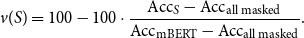 \begin{equation} v(S) = 100 - 100 \cdot \frac{\mathrm{Acc}_S - \mathrm{Acc}_{\text{all masked}}}{\mathrm{Acc}_{\text{mBERT}} - \mathrm{Acc}_{\text{all masked}}}. \end{equation}
Not only are the Shapley values defined by Equation (2) an additive measure of the contributions that a particular player (in our case, the average word occurring in that position) makes to solving the task, but they define the only such measure (Shapley, Reference Shapley1951).
7.1 Implementation
Both mBERT and XLM-RoBERTa have built-in mask tokens that are used for the MLM objective. We remove the contribution of certain tokens by replacing them with mask symbols. Multiple tokens can be removed at a time and we use a single mask token in place of each token. We designate an unused character as mask for the chLSTM experiments. When a token is masked, we replace each of its characters with this mask token. Computing the Shapley values for nine players requires $2^9=512$
experiments for each of the 247 tasks. This includes the unmasked sentence (all players contribute) and the completely masked sentence (no players), where each token is replaced with a mask symbol.
$2^9=512$
experiments for each of the 247 tasks. This includes the unmasked sentence (all players contribute) and the completely masked sentence (no players), where each token is replaced with a mask symbol.
7.2 General results
Figure 16 shows the Shapley values averaged over the 247 tasks for each model. Table 6 summarizes the numerical results. The values extracted from the two MLMs are remarkably similar. We quantify this similarity using $L_1$
(Manhattan) distance, which is 0.09 between the means.Footnote r The Shapley distributions obtained by XLM-RoBERTa and mBERT move closely together: the mean distance between Shapley values obtained from XLM-RoBERTa and mBERT is just 0.206, and of the 247 pairwise comparisons, only 5 are more than two standard deviations above the mean. This means that in general Shapley values are more specific to the morphology of the language than to the model we probe. To simplify our analysis, we only discuss the XLM-RoBERTa results in detail since they show the same tendencies and are slightly better than the results achieved with mBERT.
$L_1$
(Manhattan) distance, which is 0.09 between the means.Footnote r The Shapley distributions obtained by XLM-RoBERTa and mBERT move closely together: the mean distance between Shapley values obtained from XLM-RoBERTa and mBERT is just 0.206, and of the 247 pairwise comparisons, only 5 are more than two standard deviations above the mean. This means that in general Shapley values are more specific to the morphology of the language than to the model we probe. To simplify our analysis, we only discuss the XLM-RoBERTa results in detail since they show the same tendencies and are slightly better than the results achieved with mBERT.
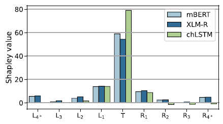
Figure 16. Shapley values by relative position to the probed target word. The values are averaged over the 247 tasks.
The first observation is that the majority of the information, 54.9%, comes from the target words themselves, with the context contributing on average only 45.1%. Next, we observe that words further away from the target contribute less, providing a window weighting scheme (kernel density function) broadly analogous to the windowing schemes used in speech processing (Harris, Reference Harris1978). Third, the low Shapley values at the two ends, summing to 11.2% in XLM-RoBERTa (11.0% in mBERT) go some way toward vindicating the standard practice in KWIC indexing (Luhn, Reference Luhn1959), which is to retain only three words on each side of the target. While the observation that this much context is sufficient for most purposes, including disambiguation and machine translation (MT), goes back to the very beginnings of information retrieval (IR) and MT (Choueka and Lusignan, Reference Choueka and Lusignan1985), our findings provide the first quantifiable statement to this effect in MLMs (for HMMs, see Sharan et al., Reference Sharan, Khakade, Liang and Valiant2018) and open the way for further systematic study directly on IR and MT downstream tasks.
With this, we are coming to our central observation, evident both from Figure 16 and from numerical considerations (Table 6): the decline is noticeably faster to the right than to the left, in spite of the fact that there is nothing in the model architecture to cause such an asymmetry (see 2.1.3). What is more, not even our experiments with random weighted MLMs (presented in Section 8.4) show such asymmetry.
Whatever happens before a target word is about 40% more relevant than whatever happens after it. In morphophonology, “assimilation” is standardly classified, depending on the direction of influence in a sequence, as progressive assimilation, in which a following element adapts itself to a preceding one, and regressive (or anticipatory) assimilation, in which a preceding element takes on a feature or features of a following one. What the Shapley values suggest for morphology is that progressive assimilation (feature spreading) is more relevant than regressive.
Table 6. Summary of the Shapley values.
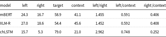
This is not to say that regressive assimilation will be impossible or even rare. One can perfectly well imagine a language where adjectives precede the noun they modify and agree to them in gender:Footnote s this form of agreement is clearly anticipatory. Also, the direction of the spreading may depend more on structural position than linear order, cf. for example the “head marking” versus “dependent marking” distinction drawn by Nichols (Reference Nichols1986). But when all is said and done, the Shapley values, having been obtained from models that are perfectly directionless, speak for themselves: left context dominates right 58.39% to 41.61% in XLM-RoBERTa (58.36% to 41.64% in mBERT) when context weights are considered 100%. This makes clear that it is progressive, rather than anticipatory, feature sharing that is the unmarked case. While our dataset is currently heavily skewed toward IE languages, so the result may not hold on a typologically more balanced sample, it is worth noting that the IE family is very broad typologically, and three of the four heaviest outliers (Hindi, Urdu, and Irish) are from IE, only Arabic is not.
7.3 Outliers
We next consider the outliers. The main outliers are listed in Figure 17. We compute the distance of each task’s Shapley values from the mean (dfm). Over 91.5% of the tasks are very close (Manhattan distance below one standard deviation, 0.264) to the mean of the distribution, and there are only five tasks (2% of the total) where the distance exceeds two standard deviations above the mean. The first row of Figure 17 shows the mean distribution and the five tasks that are closest to it, such as $\langle$
Polish, N, number
$\langle$
Polish, N, number $\rangle$
(1st row 2nd panel, distance from mean 0.053) or
$\rangle$
(1st row 2nd panel, distance from mean 0.053) or $\langle$
Lithuanian, N, case
$\langle$
Lithuanian, N, case $\rangle$
(1st row 3rd panel, dfm 0.132). These exemplify the typologically least marked, simplest cases, and thus require no special explanation.
$\rangle$
(1st row 3rd panel, dfm 0.132). These exemplify the typologically least marked, simplest cases, and thus require no special explanation.
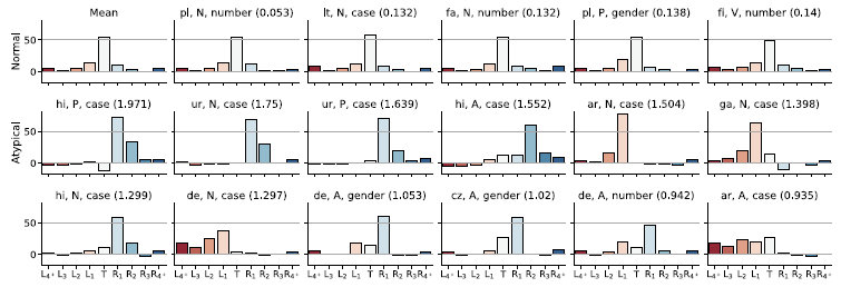
Figure 17. Least and most anomalous Shapley distributions. The first row is the mean Shapley values of the 247 tasks and the 5 tasks closest to the mean distribution, that is the least anomalous as measured by the dfm distance from the average Shapley values. The rest of the rows are the most anomalous Shapley values in descending order. For each particular task, its distance from the mean (dfm) is listed in parentheses above the graphs.
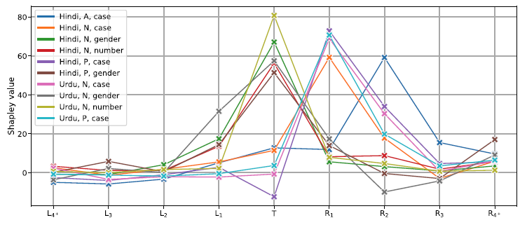
Figure 18. Shapley values in Indic tasks.
What does require explanation are the outliers, Shapley patterns far away from the norm. By distance from the mean, the biggest outliers are Indic: $\langle$
Hindi, PROPN, case
$\langle$
Hindi, PROPN, case $\rangle$
and
$\rangle$
and $\langle$
Hindi, ADJ, case
$\langle$
Hindi, ADJ, case $\rangle$
(2rd row 1st and 4th panels, dfm 1.971 and 1.552, respectively) and
$\rangle$
(2rd row 1st and 4th panels, dfm 1.971 and 1.552, respectively) and $\langle$
Urdu, NOUN, case
$\langle$
Urdu, NOUN, case $\rangle$
and
$\rangle$
and $\langle$
Urdu, PROPN, case
$\langle$
Urdu, PROPN, case $\rangle$
(2nd row 2nd and 3rd panels, dfm 1.75 and 1.639, respectively), see Figure 18. For proper nouns, the greatest Shapley contribution, about 72–73%, is on the word following the proper noun. In Hindi, not knowing the target is actually better than knowing it, the target’s own contribution is negative 12% (and in Urdu, a minuscule 3%). For the case marked on Hindi adjectives, the most important is the second to its right, 59%; followed by the 3rd to the right, 15%; the target itself, 13%; and the first to the right, 12% (we do not have sufficient data for Urdu adjectives). The Indic noun case patterns, unsurprisingly, follow closely the proper noun patterns. For both Hindi and Urdu there are good typological reasons, SOV word order, for this to be so.Footnote t
$\rangle$
(2nd row 2nd and 3rd panels, dfm 1.75 and 1.639, respectively), see Figure 18. For proper nouns, the greatest Shapley contribution, about 72–73%, is on the word following the proper noun. In Hindi, not knowing the target is actually better than knowing it, the target’s own contribution is negative 12% (and in Urdu, a minuscule 3%). For the case marked on Hindi adjectives, the most important is the second to its right, 59%; followed by the 3rd to the right, 15%; the target itself, 13%; and the first to the right, 12% (we do not have sufficient data for Urdu adjectives). The Indic noun case patterns, unsurprisingly, follow closely the proper noun patterns. For both Hindi and Urdu there are good typological reasons, SOV word order, for this to be so.Footnote t
The next biggest outliers are $\langle$
Arabic, NOUN, case
$\langle$
Arabic, NOUN, case $\rangle$
and
$\rangle$
and $\langle$
Irish, NOUN, case
$\langle$
Irish, NOUN, case $\rangle$
(Figure 17 2nd row 5th and 6th panel, dfm 1.505 resp. 1.398), where the preceding word is more informative than the target itself. These are similarly explainable, this time by VSO order. It also stands to reason that the preceding word, typically an article, will be more informative about
$\rangle$
(Figure 17 2nd row 5th and 6th panel, dfm 1.505 resp. 1.398), where the preceding word is more informative than the target itself. These are similarly explainable, this time by VSO order. It also stands to reason that the preceding word, typically an article, will be more informative about $\langle$
German, NOUN, case
$\langle$
German, NOUN, case $\rangle$
than the word itself (3nd row 2rd panel, dfm 1.297). The same can be said about
$\rangle$
than the word itself (3nd row 2rd panel, dfm 1.297). The same can be said about $\langle$
German, ADJ, gender
$\langle$
German, ADJ, gender $\rangle$
(dfm 1.053) and
$\rangle$
(dfm 1.053) and $\langle$
German, ADJ, number
$\langle$
German, ADJ, number $\rangle$
(dfm 0.942), or the fact that
$\rangle$
(dfm 0.942), or the fact that $\langle$
Czech, ADJ, gender
$\langle$
Czech, ADJ, gender $\rangle$
(3rd row 4th panel, dfm 1.02) is determined by the following word, generally the head noun.
$\rangle$
(3rd row 4th panel, dfm 1.02) is determined by the following word, generally the head noun.
If we arrange Shapley distributions by decreasing distance from the mean, we see that dfm is roughly normally distributed (mean 0.492, std 0.264). Only 21 tasks are more than one standard deviation above the mean, the last two rows of Figure 17, present the top 12 of these. Altogether, there was a single case where $R_2$
dominated,
$R_2$
dominated, $\langle$
Hindi, ADJ, case
$\langle$
Hindi, ADJ, case $\rangle$
, 16 cases when
$\rangle$
, 16 cases when $L_1$
dominates, and 11 cases where
$L_1$
dominates, and 11 cases where $R_1$
dominates, everywhere else it is the target that is the most informative. The typologically unusual patterns, all clearly related to the grammar of the language in question, are transparently depicted in the Shapley patterns. For example, as noted in Section 5.3, the article preceding the noun in German often is the only indication of the noun’s case. The Shapley values we obtained simply quantify this information dependence. Similarly, Arabic cases are determined in part by the preceding verb and/or preposition. Quite often, Shapley values confirm what we know anyway, for example that verbal tasks rely more on the target word than nominal tasks.
$R_1$
dominates, everywhere else it is the target that is the most informative. The typologically unusual patterns, all clearly related to the grammar of the language in question, are transparently depicted in the Shapley patterns. For example, as noted in Section 5.3, the article preceding the noun in German often is the only indication of the noun’s case. The Shapley values we obtained simply quantify this information dependence. Similarly, Arabic cases are determined in part by the preceding verb and/or preposition. Quite often, Shapley values confirm what we know anyway, for example that verbal tasks rely more on the target word than nominal tasks.
Another noticeable statistical trace of rule-governed behavior is seen in Hindi and Urdu, where the oblique case appears only when governed by a postposition. Therefore, the presence of a postposition in $R_1$
is diagnostic for the case of a target noun, and its presence in
$R_1$
is diagnostic for the case of a target noun, and its presence in $R_2$
is diagnostic for a target adjective. This conclusion is confirmed by the Shapley values, which are dominated by
$R_2$
is diagnostic for a target adjective. This conclusion is confirmed by the Shapley values, which are dominated by $R_1$
for case in Hindi nouns and proper nouns (67.7% and 64.9%, respectively) and by
$R_1$
for case in Hindi nouns and proper nouns (67.7% and 64.9%, respectively) and by $R_2$
for Hindi adjectives (82%). Urdu noun and proper noun cases show the same
$R_2$
for Hindi adjectives (82%). Urdu noun and proper noun cases show the same $R_1$
dominance (64.4% and 68.5%). In contrast, the overall average Shapley value of
$R_1$
dominance (64.4% and 68.5%). In contrast, the overall average Shapley value of $R_1$
and
$R_1$
and $R_2$
is only 10.4% and 2.9% (see Figure 18 for the full patterns).
$R_2$
is only 10.4% and 2.9% (see Figure 18 for the full patterns).
To the extent that similar rule-based explanations can be ascertained for all cases listed in Figure 17, we can attribute XLM-RoBERTa’s success to an impressive sensitivity to grammatical regularities. Though the mechanisms are clearly different, such a finding places XLM-RoBERTa in the same broad tradition as other works seeking to discover rules and constraints (e.g., Brill, Reference Brill1993).
7.4 The difficulties of generalization
Our Shapley data can be summarized as a nine-dimensional vector for each $\langle$
i, j, k
$\langle$
i, j, k $\rangle$
. In other words, the Shapley distributions come naturally arranged in a 3D tensor. Unfortunately, many of the values are missing, either because the language does not combine a particular POS with a particular tag, or because we do not have enough data for training on the task. With a much larger dataset (recall from Section 3.1 that we use essentially all currently available uniformly coded data) experimenting with 3D tensor decomposition techniques (Kolda and Bader, Reference Kolda and Bader2009) may make sense, but for now the outcome depends too much on the imputation method. That said, we have obtained one robust conclusion, independent of how we fill the missing values: it is harder to generalize by language than by POS or tag. It would be tempting to look at languages as units of generalization, but we found that trends rarely apply to individual languages!
$\rangle$
. In other words, the Shapley distributions come naturally arranged in a 3D tensor. Unfortunately, many of the values are missing, either because the language does not combine a particular POS with a particular tag, or because we do not have enough data for training on the task. With a much larger dataset (recall from Section 3.1 that we use essentially all currently available uniformly coded data) experimenting with 3D tensor decomposition techniques (Kolda and Bader, Reference Kolda and Bader2009) may make sense, but for now the outcome depends too much on the imputation method. That said, we have obtained one robust conclusion, independent of how we fill the missing values: it is harder to generalize by language than by POS or tag. It would be tempting to look at languages as units of generalization, but we found that trends rarely apply to individual languages!
For the totality of tasks $\langle$
i, j, k
$\langle$
i, j, k $\rangle$
, we can keep one of
$\rangle$
, we can keep one of $i,j$
, or
$i,j$
, or $k$
fixed and compute the average Shapley distributions
$k$
fixed and compute the average Shapley distributions $S_{j,k}(i), S_{i,k}(j)$
, and
$S_{j,k}(i), S_{i,k}(j)$
, and $S_{i,j}(k)$
. Given the average distributions, say
$S_{i,j}(k)$
. Given the average distributions, say $S_{j,k}$
(Polish) we can ask how far Shapley distributions for all available Polish tasks are from it and compute the average of these distances from the mean in the selected direction (in this case, language). We find that the average distance from the language averages is 0.37, while the distance from tag averages is 0.25 and the distance from POS averages is 0.26. In other words, aggregating tasks by language results in considerably larger variability than aggregating by POS or tag. The POS and tag results are similar since POS and tag are highly predictive of each other across languages: typically nouns will have case, verbs will have tense, and conversely, tenses are found on verbs, cases on nouns. This makes data aggregated on POS and tag jointly, as in Figure 11, much easier to make sense than data aggregated by language.
$S_{j,k}$
(Polish) we can ask how far Shapley distributions for all available Polish tasks are from it and compute the average of these distances from the mean in the selected direction (in this case, language). We find that the average distance from the language averages is 0.37, while the distance from tag averages is 0.25 and the distance from POS averages is 0.26. In other words, aggregating tasks by language results in considerably larger variability than aggregating by POS or tag. The POS and tag results are similar since POS and tag are highly predictive of each other across languages: typically nouns will have case, verbs will have tense, and conversely, tenses are found on verbs, cases on nouns. This makes data aggregated on POS and tag jointly, as in Figure 11, much easier to make sense than data aggregated by language.
8. Ablations
In this section, we empirically consider the criticisms raised in Belinkov (Reference Belinkov2022) and Ravichander et al. (Reference Ravichander, Belinkov and Hovy2021) for probing setups like ours. Our first group of tests (Section 8.1) confirms that the probing accuracy does not depend on the choice of probe, in particular, linear probes are no better or worse than non-linear ones. We also show that probing individual layers of mBERT or XLM-RoBERTa is worse or no better than probing the weighted sum of all layers (Section 8.2). We also show that fine-tuning decreases the probing accuracy while it substantially increases the computational requirements (Section 8.3). Finally, we show that probing a randomly initialized model, a control used by Voita and Titov (Reference Voita and Titov2020), is significantly worse than probing the trained model (Section 8.4). We present all results averaged over all 247 tasks in this section. With the exception of Section 8.4, we do not perturb the input sentences.
8.1 Linear probing and MLP variations
The probes we presented so far all use an MLP with a single hidden layer with 50 neurons. The input is the weighted sum of the 12 layers and the embedding layer with learned weights. The size of the output layer depends on the number of classes in the probing tasks. We use ReLU activations in the MLP.
The original BERT paper (Devlin et al., Reference Devlin, Chang, Lee and Toutanova2019) used a simple linear classification layer with weight $W \in \mathbb{R}^{K \times H}$
, where
$W \in \mathbb{R}^{K \times H}$
, where $K$
is the number of labels and
$K$
is the number of labels and $H$
is the hidden size of BERT, 768 in the case of mBERT and XLM-RoBERTa. Hewitt and Liang (Reference Hewitt and Liang2019) argue that linear probes have high selectivity, that is they tend to memorize less than non-linear probes. We test this on our dataset with two kinds of linear probes. The first one is the same as the general probing setup but we remove the ReLU activation. The second one completely removes the hidden layer similarly to the original BERT paper. We also test two MLP variations, one with 100 hidden size instead of 50 and another one with two hidden layers.
$H$
is the hidden size of BERT, 768 in the case of mBERT and XLM-RoBERTa. Hewitt and Liang (Reference Hewitt and Liang2019) argue that linear probes have high selectivity, that is they tend to memorize less than non-linear probes. We test this on our dataset with two kinds of linear probes. The first one is the same as the general probing setup but we remove the ReLU activation. The second one completely removes the hidden layer similarly to the original BERT paper. We also test two MLP variations, one with 100 hidden size instead of 50 and another one with two hidden layers.
Figure 19 shows the accuracy of the two linear probes and the larger MLPs as the difference from the default version we used elsewhere. These numbers are averaged over that 247 tasks. The differences are all smaller than 0.25% points. These results indicate that the probing accuracy does not depend on the probe type and particularly that linear probes perform similarly to non-linear ones.
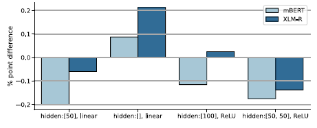
Figure 19. The average probing accuracy using different MLP variations. We indicate the size(s) of hidden layer(s) in square brackets.
8.2 Layer pooling
Our default setup uses a weighted sum of the 12 layers and the embedding layers, one scalar weight for each of them with a total of 13 learned weights. It has been shown (Tenney, Das, and Pavlick, Reference Tenney, Das and Pavlick2019a) that the different layers of mBERT work better for different tasks. Lower layers work better for low-level tasks such as POS tagging, while higher layers work better for higher-level tasks such as coreference resolution. Morphosyntactic tagging is a low-level task. The embedding layer itself is often indicative of the morphological role of a token. We test this by probing each layer separately as well as probing the concatenation of all layers.
Figure 20 shows the difference between probing the weighted sum of all layers and probing individual layers averaged over all tasks. We observe approximately 10% point difference in the embedding layer (layer 0) and the lower layers. This difference gradually decreases, and it is close to 0 in the upper layers. Our results support the finding of Hewitt et al. (Reference Hewitt, Ethayarajh, Liang and Manning2021) that morphosyntactic cues are encoded much higher into the layersFootnote u then previously suggested by Tenney et al. (Reference Tenney, Das and Pavlick2019a), discussed in Hewitt and Liang (Reference Hewitt and Liang2019). Layer concatenation (concat) is slightly better than the weighted sum of the layers, but it should be noted that the parameter count of the MLP is an order of magnitude larger thanks to the 13 times larger input dimension.
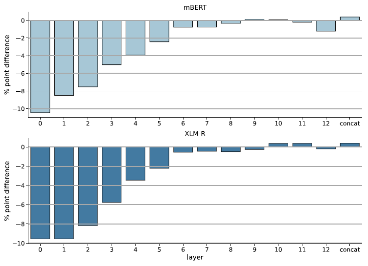
Figure 20. The difference between probing a single layer and probing the weighted sum of layers. concat is the concatenation of all layers. 0 is the embedding layer. Large negative values on the y-axis mean that probing the particular layer on the x-axis is much worse than probing the weighted sum of all layers.
We also observe that the gap between the embedding layer (layer 0) and the first Transformer layer (layer 1) is much smaller in the case of XLM-RoBERTa than mBERT. XLM-RoBERTa’s embedding layer is significantly better than mBERT’s embedding layer to begin with (82.2% vs. 80%), and this gap shrinks to 0.3% point at the first layer (82.2% and 81.9%). This is more evidence for one of our main observations that XLM-RoBERTa’s embedding and vocabulary are better than those of mBERT’s.
8.3 Fine-tuning
Fine-tuning (as opposed to feature extraction) trains all BERT parameters along with the MLP in an end-to-end fashion. This raises the number of trainable parameters from 40k to over 170M. The recommended optimizer for fine-tuning BERT models is AdamW (Loshchilov and Hutter, Reference Loshchilov and Hutter2019), a variant of the Adam optimizer. We try both Adam and AdamW for fine-tuning the model on each task and show that AdamW is indeed a better choice than Adam (Table 7), but nevertheless the feature extraction results are 0.5 percentage point better than the fine-tuning results and this difference is statistically significant. Our experiments also show that the running time is increased 80-fold when we fine-tune mBERT. Due to this increase in computation time, we do not repeat the experiments for XLM-RoBERTa. It should be noted that BERT fine-tuning has its own tricks (Houlsby et al., Reference Houlsby, Giurgiu, Jastrzebski, Morrone, De Laroussilhe, Gesmundo, Attariyan and Gelly2019; Li and Liang, Reference Li and Liang2021; Ben Zaken, Goldberg, and Ravfogel, Reference Ben Zaken, Goldberg and Ravfogel2022) that may lead to better results but we do not explore them in this paper.
Table 7. Comparison of fine-tuned and frozen (feature extraction) models.
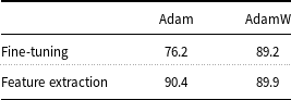
8.4 Randomly initialized MLMs
Randomly initialized language models have been widely used as a baseline when evaluating language models (Conneau et al., Reference Conneau, Kiela, Schwenk, Barrault and Bordes2017), especially via auxiliary classifiers (Zhang and Bowman, Reference Zhang and Bowman2018; Conneau et al., Reference Conneau, Kruszewski, Lample, Barrault and Baroni2018a; Htut et al., Reference Htut, Phang, Bordia and Bowman2019; Voita and Titov, Reference Voita and Titov2020). Zhang and Bowman (Reference Zhang and Bowman2018) showed that the mechanism of assigning morphosyntactic tags to these random embeddings is significantly different. As they demonstrated, randomly initialized MLMs rely on word identities, while their trained counterparts maintain more abstract representations of the tokens in the input layer. Therefore, probing classifiers applied on random MLMs may pick up low-level patterns only, such as word identity, and this could mislead the probing controls when used as a baseline.
In order to test this hypothesis, we trained the probing classifiers using randomly initialized mBERT and XLM-RoBERTa models. In this setup, both fully random and pre-trained embedding layer with random Transformer layers were compared to trained MLMs.
Table 8 shows the overall probing accuracy achieved on random models. We add the majority (most frequent) baseline as a comparison. Although the random MLMs are clearly better than the majority baseline, they are far worse than the trained MLMs.
Table 8. Probing accuracy on the randomly initialized mBERT and XLM-RoBERTa models.
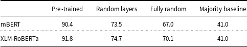
Figure 21 shows that neither b $_{2}$
, l
$_{2}$
, l $_{2}$
, r
$_{2}$
, r $_{2}$
nor permute perturbations affect the model’s performance in a way that they do when applied on the trained models (compare Figure 8). Nevertheless, this sub-experiment offers two further supporting arguments for the claims Zhang and Bowman (Reference Zhang and Bowman2018) made about random MLMs learning word identities:
$_{2}$
nor permute perturbations affect the model’s performance in a way that they do when applied on the trained models (compare Figure 8). Nevertheless, this sub-experiment offers two further supporting arguments for the claims Zhang and Bowman (Reference Zhang and Bowman2018) made about random MLMs learning word identities:
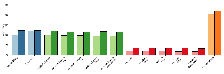
Figure 21. Random mBERT (light color) and random XLM-RoBERTa (darker color) performance comparison with different perturbation setups and the unperturbed trained model variants (orange bars). Left-to-right: Blue: Accuracy of the embedding and first layers’ probes; Green: Random models with pre-trained embedding layer: no perturbation, b $_{2}$
, l
$_{2}$
, l $_{2}$
, r
$_{2}$
, r $_{2}$
, permute; Red: Random models where the embedding layer is random as well: no perturbation, b
$_{2}$
, permute; Red: Random models where the embedding layer is random as well: no perturbation, b $_{2}$
, l
$_{2}$
, l $_{2}$
, r
$_{2}$
, r $_{2}$
, permute; Orange: Unperturbed trained models.
$_{2}$
, permute; Orange: Unperturbed trained models.
-
1. The accuracies of random models’ morphological probes match the accuracies of their embedding layers’ probe; that is even the Transformer-based random MLMs rely mostly on the word identities represented by their embeddings
-
2. Probing perturbed and unperturbed embeddings of random MLMs does not make a big difference (the accuracies of unperturbed and perturbed models’ are less than 1% apart). Clearly, word identities count the most, their order almost not at all.
Based on this finding, we do not use randomized MLMs as baselines.
8.5 Training data size
Our sampling method (cf. Section 3.2) generates 2,000 training samples. Raising this number would remove many tasks from languages with smaller UD treebanks. Probing methods on the other hand are supposed to test the already existing linguistic knowledge in the model; therefore, probing tasks’ training sets should not be too large. In this section, we show that smaller training sizes result in inferior probing accuracy. Our choice of 2000 samples was a practical upper limit that allowed for a large number of tasks from mid-to-large-sized UD treebanks.
Figure 22 shows the average accuracy of the probing tasks when we use fewer training samples. Although the probing tasks work considerably better than the majority baseline even with 100 sentences, the overall accuracy gets better as we increase the training data. Interestingly, XLM-RoBERTa is always slightly better than mBERT.
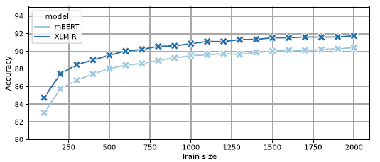
Figure 22. Probing accuracy with reduced training data.
9. Discussion
Throughout this paper, we analyzed a large number of experiments and a few trends were clear and corroborated by various experiments. In this section, we summarize these observations and point back to the experiments that confirm them.
Pre-training learns morphology
Morphology is a low-level task, and for the most part, it is considered an easy task as evidenced by the success of small encoder-decoder networks in the SIGMORPHON shared tasks on token-level morphology. Our strongest baseline, chLSTM, which is not pre-trained on external data but only on the 2000 training sentences from the probing data, performs reasonably well on most morphosyntactic tasks. We still find that the MLMs and Stanza offer significant improvement, which can only be attributed to the their far larger training set (Table 2). chLSTM is only better at eight tasks out of the 247, and the difference is never large. The difference is not uniform across tags and POS (Figures 3 and 4) and neither is it uniform across language families. MLMs are much better at Slavic tasks (Figure 5). MLMs also struggle with some tasks (Section 5.3) but these tasks seem to be even more difficult for chLSTM.
Another proof of the effect of pre-training is the subpar performance of random models (Section 8.4). We try two kinds of randomized models (with and without randomized embedding) and both are much worse than their pre-training counterparts regardless of which MLM we use. Perturbations do not seem to affect the results when using randomized models, suggesting that the random models mostly rely on word identities rather than some higher-level morphosyntactic knowledge (Figure 21).
Left context plays a bigger role in morphosyntax than right context
One of our main findings is that the left context plays a more important role in morphosyntax than the right context and this seems to hold for most languages. The relative importance of the left context is clearly observed in both MLMs and in chLSTM (Table 6). Considering that all three models are architecturally symmetrical, we can conclude that this is due to linguistic reasons rather than some modeling bias. The simplest way we show that the left context is more important is via the context masking perturbations that mask words on the left, the right or both sides of the target word. The effect of l $_{2}$
is clearly larger than r
$_{2}$
is clearly larger than r $_{2}$
(c.f. Table 5) for all three models. l
$_{2}$
(c.f. Table 5) for all three models. l $_{2}$
is larger than r
$_{2}$
is larger than r $_{2}$
for all of the large language families (Figure 10) in our dataset, although all context masking has negligible effect on Uralic tasks. We further quantify the role of each contextual word in Section 7 and discuss some notable exceptions, particularly from the Indic family.
$_{2}$
for all of the large language families (Figure 10) in our dataset, although all context masking has negligible effect on Uralic tasks. We further quantify the role of each contextual word in Section 7 and discuss some notable exceptions, particularly from the Indic family.
XLM-RoBERTa’s embedding and vocabulary are better suited for multilingual morphology than mBERT’s
Given that XLM-RoBERTa’s subword vocabulary is twice as large as mBERT’s, we can expect more language-specific subwords especially for low-resource languages. We show three qualitative evidence that the embedding of XLM-RoBERTa is actually better than the embedding of mBERT and we are reasonably certain that this cannot be attributed to differences in the pre-training corpora, since the gap shrinks in the higher layers. First, we find that the average probing accuracy at the embedding layer (Section 8.2) not only is higher for XLM-RoBERTa than mBERT but the performance drop in comparison to using the weighted sum of all layers is smaller for XLM-RoBERTa than mBERT. Second, there is very little improvement between probing the embedding layer of XLM-RoBERTa and its first Transformer layer. This is not the case for mBERT, where we see a larger improvement (c.f. Figure 20). And third, the randomized models show that not randomizing the embedding layer leads to superior performance by XLM-RoBERTa compared to mBERT.
Trends pertain to specific morphosyntactic tags rather than languages
Our extensive experiments show various trends and the languages themselves are rarely the best unit for drawing general conclusions such as one model being better than the other at a particular language. We find that morphosyntactic tags and POS tags are both better choices as the units of generalization. Whenever we group the results by language family (Figures 10 and 12), the standard deviations are often larger than the effects themselves.
We see examples where cross-POS comparison is meaningful, for example adjective tasks rely on the context more than noun and verbal tasks do (in other words, targ has smaller effect on adjectives, see 6.1.2). But not all POS categories lend themselves to similar generalizations; in particular, proper nouns are hard to make sense of as a cross-linguistically valid grouping.Footnote v We also show various individual examples where the tag, particularly case, is a much better generalization horizon than the language itself (Figures 3 and 10).
In Section 7.4, we show quantitative proof for this claim by computing the variance of the Shapley values as a function of the unit of generalization. We find that language is a worse generalizing factor than both tag and POS.
10. Conclusions
We introduced a dataset of 247 probing tasks, covering 42 languages from 10 families. Using the dataset, we demonstrated that mBERT and XLM-RoBERTa embody considerable morphological knowledge, reducing errors by a third compared to task-specific baselines with the same number of trained parameters and generally performing at a high level even after masking portions of the input.
Our main contribution is the detailed analysis of the role of the context by means of perturbations to the data and Shapley values. We find that, for this large suite of tasks, the information resides dominantly in the target word, and that left and right contexts are not symmetrical, morphological processes are more forward spreading than backward spreading.
Acknowledgements
We are grateful for the anonymous reviewers’ insightful criticism, inquiries that prompted more discussion in the text, and high-quality references. This work was partially supported by the European Union project RRF-2.3.1-21-2022-00004 within the framework of the Artificial Intelligence National Laboratory Grant no RRF-2.3.1-21-2022-00004. Judit Ács was partially supported by the Fulbright Scholarship and the Rosztoczy Scholarship. Endre Hamerlik was partially supported by grant APVV-21-0114 of the Slovak Research and Development Agency and Visegrad Scholarship nr.: 52110970.
Competing interests
The authors declare none.
Appendix A. Dataset statistics
The dataset creation method and the choice of languages and tags are described in Section 3. Here we list some additional statistics.
Our sampling method limits the sentence length between 3 and 40 tokens. The average sentence length is 20.5 tokens. The subword tokenizer of mBERT generates 38.2 tokens on average, while the subword tokenizer of XLM-RoBERTa outputs 34.2 tokens. Target fertility is defined as the number of subwords the target token is split into. Target fertility is 3.1 and 2.6 for mBERT and XLM-RoBERTa, respectively. However, this measure varies substantially among languages, particularly in the case of mBERT’s tokenizer. mBERT generates the fewest subwords for target words in English (2.05) and the most for Greek (4.75). XLM-RoBERTa on the other hand tends to split Persian the least (2.05) with English coming second (2.14), and it splits Hungarian the most (3.21), and the target fertility for all other languages is below 3 for XLM-RoBERTa. mBERT’s target fertility is above 3 for 22 out of the 42 languages. This again suggests that XLM-RoBERTa’s larger vocabulary is better suited for a multilingual setup.
Lastly, we analyze the target words in more detail. Our data creation method disallows having the same target word appear in more than one of the train, validation, or test splits. If the example sentence “I read your letter yesterday.” is part of the train set and read is the target word, it may not appear as a target word in the validation or the test set regardless of its morphosyntactic analysis. It may be part of the rest of the sentence though. A probing task has 2024 unique target words on average. Split-wise this number is 1644 for the train split, 189 for the validation split, and 190 for the test split. Recall that we have 2000 train, 200 validation, and 200 test sentences. Interestingly, there is very little ambiguity in the morphosyntactic analysis of the 4 tags we consider. 6.5% of words have ambiguous analysis in the full UD treebanks of the 42 languages.
Appendix B. Stanza setup
Stanza is a collection of linguistic analysis tools in 70 languages trained on UD treebanks. Stanza is an ideal tool for comparison since it was trained on the same dataset we use to sample our probing tasks. The underlying model is a highway bidirectional LSTM (Srivastava, Greff, and Schmidhuber, Reference Srivastava, Greff and Schmidhuber2015) with inputs coming from the concatenation of word2vec or fastText vectors, an embedding trained on the frequent words of UD and a character-level embedding generated by a unidirectional LSTM. We use the default models available for each language.
It works in a pipeline fashion, and one of its intermediate steps is morphosyntactic analysis in UD format. We use this analysis as a high-quality baseline for all of our 42 languages and 247 tasks except Albanian (six tasks). We apply Stanza on the full probing sentences, and we extract the morphosyntactic analysis of the target words. Since Stanza’s own tokenizer often outputs a different tokenization than UD’s gold tokenization, we extract every overlapping token and check the union of the morphosyntactic tags if there is more than one such overlapping token. This results in a set of Feature=Value pairs. We extract each occurrence of the feature of the particular probing task. If there is only one and it is the same as the reference label, it is correct. If there are more than one values and the correct value is among them, we divide one by the number of distinct values. In practice, this is very rare; 91% of the time, there is only one value in it that is the same as the reference value. 8.3% of the time the reference value is not in the analysis of Stanza. The remaining 0.7% are the cases where there are multiple values including the correct one.
Appendix C. Layer weights
We use scalar weighting for the 12 Transformer layers and the embedding layer. The 13 scalar weights are learned for each probing experiment along with the MLP weights. We use the softmax function to produce a probability distribution for the layer weights. Our analysis shows that the layer distribution is very close to the uniform distribution. We quantify this in two ways: the ratio of the highest and the lowest layer weight and the entropy of the weight distribution. The two measures highly correlate (0.95 Pearson correlation). The highest ratio of the largest and smallest layer weight is 2.22 for mBERT and 2.24 for XLM-RoBERTa, while the lowest entropy is 3.62 for both models (the entropy of the uniform distribution is 3.7). We list the 50 task with the highest max-min ratio in Figure 23. Interestingly, the higher layers are weighted higher in each of the 50 outlier tasks somewhat contradicting the notion that low-level tasks such as morphology use lower layers of BERT (Tenney, Das, and Pavlick, Reference Tenney, Das and Pavlick2019a).
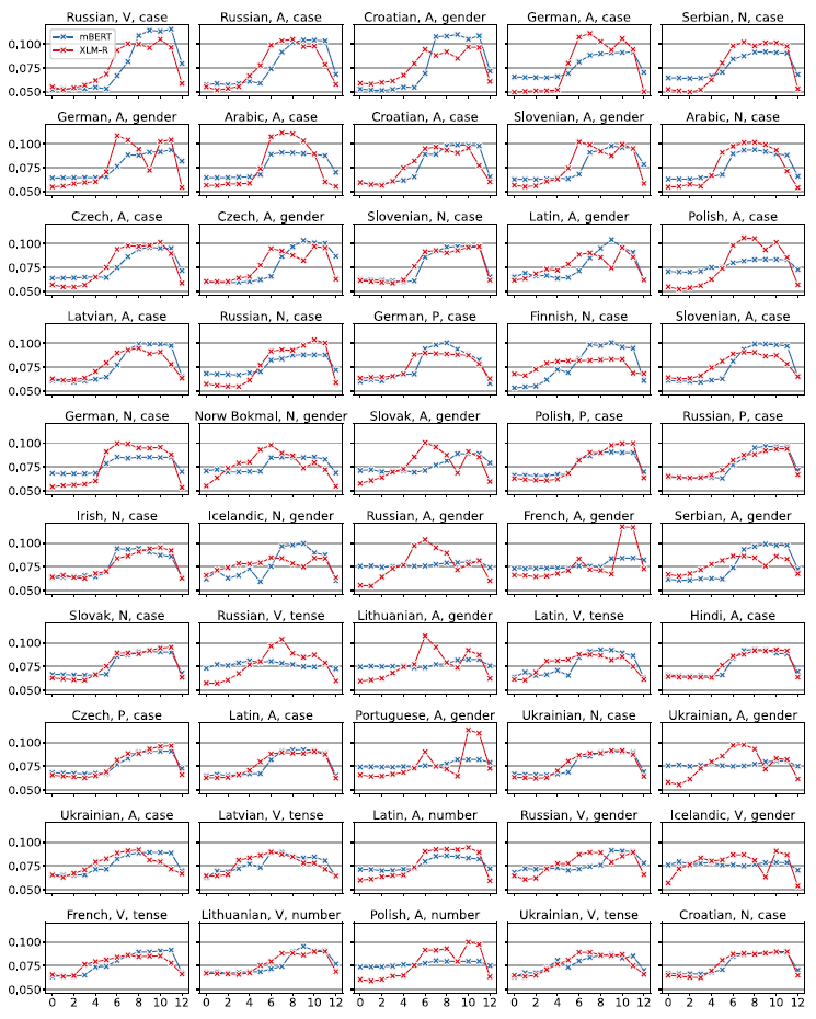
Figure 23. Layer weight outliers. Layer 0 is the embedding layer.
We also found that the two models show similar patterns task-wise. When the layer weights corresponding to one task have a lower entropy, they tend to have a lower entropy when we probe the other model too. The ranking of the entropy of the 247 tasks’ weights confirms this (0.63 Spearman’s rank correlation). We did not find any significant pattern pertaining to a particular language or language family.
Appendix D. Additional Shapley figures
We include extra figures and analysis for the Shapley value analysis from Section 7.
Figure 24 shows the Shapley values by POS. Adjectives and proper nouns rely on the context more than common nouns or verbs. We see similar trends when we look at the per-tag Shapley values in Figure 25. Tense, an exclusively verbal tag, has the largest Shapley value for target out of the four tags.
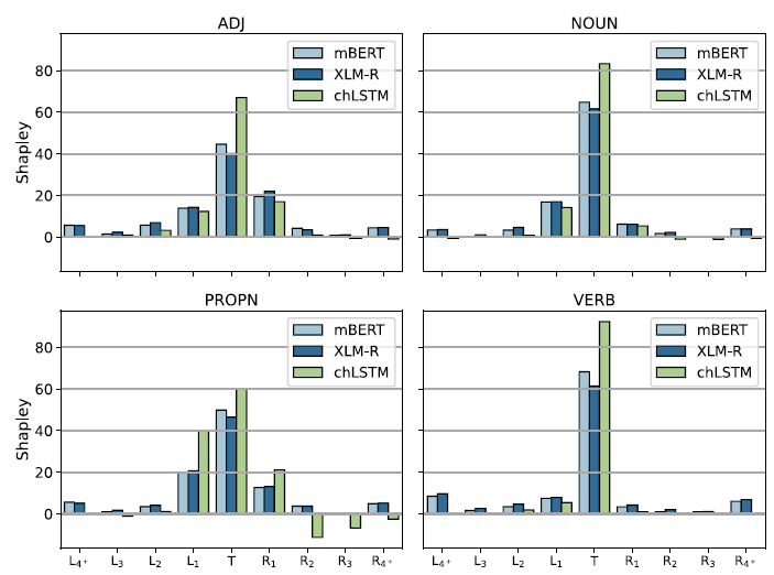
Figure 24. Shapley values by POS and model.
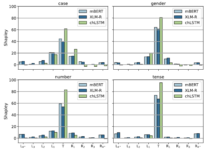
Figure 25. Shapley values by POS and model.
Finally, we opted to mention the curious case of German tasks depicted in Figure 26. German is clearly the biggest outlier from the Germanic family. In fact, it is dissimilar to every other language as illustrated by our clustering experiments (c.f. Figure 15). Multiple German tasks appear in the main Shapley outliers (Figure 17) and among the tasks with the least uniform layer weights (Figure 23). When looking at the individual tasks’ Shapley values, only 4 of the 10 German tasks are dominated by the target. Case tasks are left dominant, while adjective gender and number rely on $R_1$
the most.
$R_1$
the most.
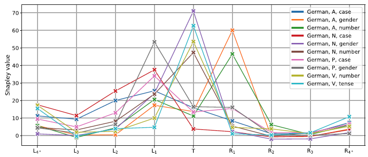
Figure 26. Shapley values in German tasks.
Appendix E. Computational requirements
We run every unperturbed and perturbed experiment 10 times and report the average of the 10 runs. The Shapley value computation requires $2^9=512$
experiments for each model and each task; we only run them once. Experiments related to the ablations are also run once. The overall number of experiments we ran is 460k. The average runtime of an experiment is 7 s, and the total runtime is roughly 38 days on a single GPU. We used a GeForce RTX 2080 Ti (12 GB) and a Tesla V100 (16 GB). The maximum number of epochs was set to 200, but in practice this is only reached in 2% of the experiments. Early stopping based on the development loss ends the experiments after 22 epochs on average.
$2^9=512$
experiments for each model and each task; we only run them once. Experiments related to the ablations are also run once. The overall number of experiments we ran is 460k. The average runtime of an experiment is 7 s, and the total runtime is roughly 38 days on a single GPU. We used a GeForce RTX 2080 Ti (12 GB) and a Tesla V100 (16 GB). The maximum number of epochs was set to 200, but in practice this is only reached in 2% of the experiments. Early stopping based on the development loss ends the experiments after 22 epochs on average.


 Open access