


Introduction
The Groningen gas field
A few years after its discovery in 1959 it was realised that the Groningen field was one of the largest gas fields in the world. It has an extent of roughly 45 by 25km laterally. The volume of gas initially in place (GIIP) is estimated at 2900 billion normal cubic metres (Gnm3=bcm). Production started in 1963. Since then, a total of 326 production wells in 26 clusters had produced a total volume of 2166bcm by 31 December 2016. In 2016 258 wells and 22 clusters were still active and production amounted to 27.6bcm. Initially the reservoir pressure was 347bar and it now varies between 70 and 95bar depending on the location in the field. The gas is produced from the Slochteren formation (of Permian age), a sandstone reservoir at a depth ranging from 2700 to 3000m. This producing interval has a gross thickness in the range 168–225m. Average porosity ranges from 13% to 16%, and average permeability from 82 to 122mDarcy, depending on the sedimentological facies. The Slochteren formation comprises both fluvial and aeolian deposits. A more detailed geological description of the Rotliegend petroleum play of the Netherlands and the heterogeneity of this reservoir is given by de Jager & Geluk (Reference de Jager, Geluk, Wong, Batjes and de Jager2007). An abundance of faults intersect the reservoir. This plays an important role in the Groningen field (Kortekaas & Jaarsma, Reference Kortekaas and Jaarsma2017). A NAM study (2016a) described 1500 mapped faults and the report concludes that these faults do not significantly influence the permeability at large. However, it is also recognised that dynamic reservoir modelling requires taking into account fault (zone) properties and calibrating the transmissibility of different faults to obtain the best history match on production, pressure, water rise and subsidence data. As a result, some degree of compartmentalisation is also shown by streamline maps that indicate the flow path of gas molecules to the different production clusters (NAM, 2016b).
Production history
Figure 1 shows the production history of the field. During the 1960s and 1970s the field was rapidly developed until it reached its maximum annual production of 87.7bcm in 1976. Because of the government's policy to give priority to the development of the other (smaller) gas fields in the Netherlands, Groningen's annual production was reduced until around the year 2000. Thereafter it became necessary to increase production again in order to compensate for the then declining total gas production from the small fields in the Netherlands.
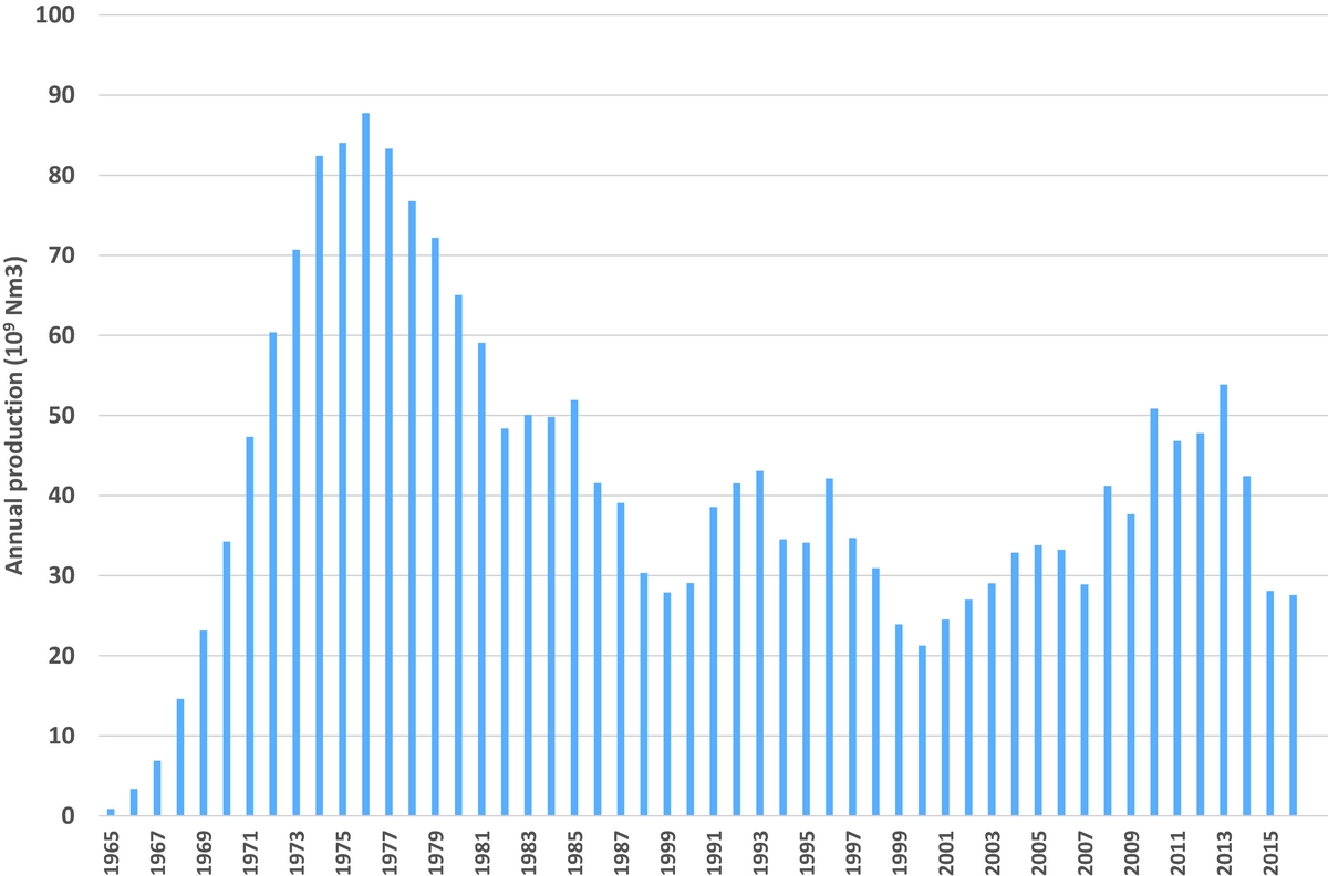
Fig. 1. Annual gas production from the Groningen field since 1965.
After a substantial increase in public concern resulting from the earthquake near Huizinge (M=3.6 on 16 August 2012, the largest seismic event until today) more research was performed in 2013. In the light of this event, the Minister of Economic Affairs decided in January 2014 to impose stricter limits on annual production. The maximum permitted annual production was reduced in a few steps after 2014. The result of these measures in terms of annual production is shown in Figure 1. At this moment the limit is set at a production level of 24bcm per gas year, i.e., the period from 1 October 2016 to 30 September 2017.
A specific characteristic of gas production from the Groningen field has been the large seasonal variation in production (Fig. 2). With the demand being high in winter and low in summer, the field played the role of ‘swing producer’ for the Dutch gas market, while the Dutch small fields produced the base load. Since the decline in production from the small fields and the extension of underground gas storages in the Netherlands which are filled during the summer, more production was needed during the summer period from the Groningen field in the more recent years.
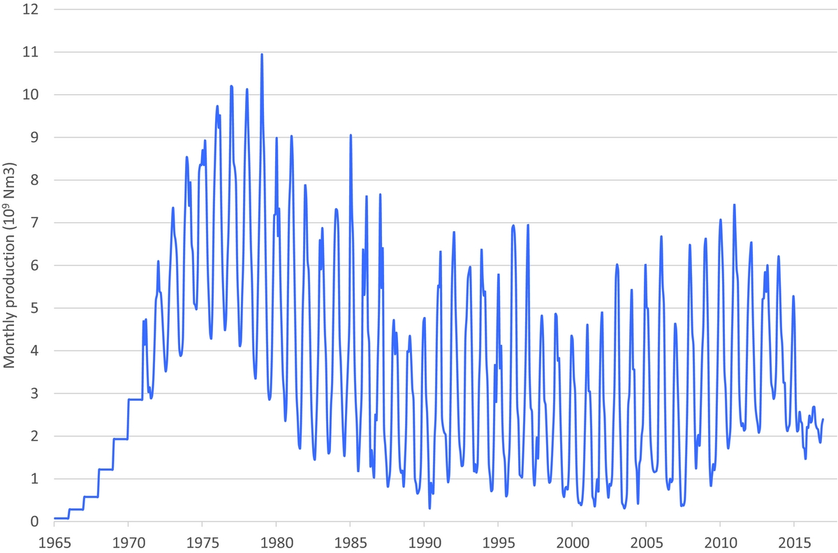
Fig. 2. Monthly production (as high as 10bcm in a winter month in the 1970s).
Observed seismicity history
The authority responsible for the registration of earthquakes in the Netherlands (KNMI (Royal Netherlands Meteorological Institute)) has not registered an earthquake in the north of the Netherlands prior to 1986. The region has always been considered tectonically inactive, and hence the earthquakes observed since 1986 (the first observed earthquake being near Assen, but outside the Groningen field) are interpreted to be induced (van Eck et al., Reference van Eck, Goutbeek, Haak and Dost2006; Dost & Haak, Reference Dost, Haak, Wong, Batjes and de Jager2007). The first registered event attributed to the Groningen field occurred near Middelstum on 5 December 1991 and had a magnitude of M=2.4 on the Richter scale. By that time, average pore pressure in the reservoir (reservoir pressure) had decreased to about 180bar. In response to concerns raised after the first tremors, KNMI gradually extended its seismic monitoring network for the Groningen field over time (Dost et al., Reference Dost, Goutbeek, Van Eck and Kraaijpoel2012). The result of these extensions was a stepwise decrease in the detection limit.
Van Thienen-Visser et al. (2016) performed a statistical analysis to determine the development of the magnitude of completeness, where magnitude of completeness is defined as the lowest magnitude that has a 95% probability of being detected in three or more borehole stations. They concluded that for the period 1996–2009 a magnitude of completeness of M=1.5 can be assumed. The magnitude of completeness has decreased to M=1.3 for almost the entire field since 2010 when the network was extended and was also M=1.3 for the largest part of the field where most of the seismicity occurs before 2010. A further lowering of the detection limit can be expected from the most recent extension of the monitoring network. Since 2014 this has consisted of 70 shallow borehole stations at depths of 50, 100 and 200m, equipped with geophones and seismographs at the surface. When doing statistical analyses on the entire seismic catalogue, a cut-off value of M=1.5 is often used (e.g. NAM, 2016a). Considering only more recent periods, cut-offs of either M=1.3 or even M=1.0 can be used, but care should be taken when making comparisons.
Figure 3 shows the number of recorded events for each year and also shows when the stronger earthquakes occurred. Much of the debate during the last four years has been about attempts to relate the observed changes in annual seismic activity (Fig. 3) to changes in annual production volume (Fig. 1). Success in trying to influence the seismic activity rate (and hence seismic hazard and risk) by controlling production rates and their spatial distribution depends on a good description of the relationship between the two.
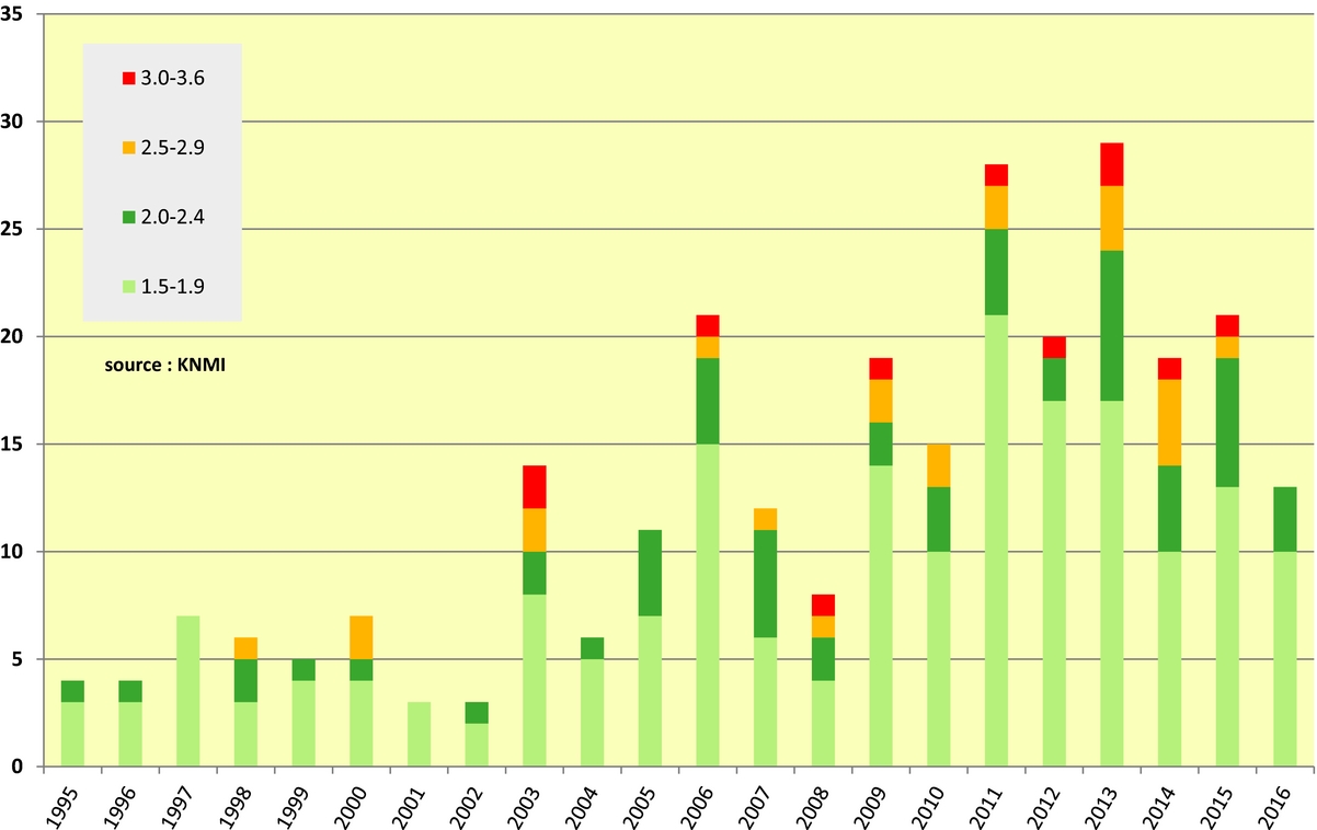
Fig. 3. Registered induced earthquakes from the Groningen field since 1995, with a lower limit of M=1.5 and subdivided into four classes according to magnitude.
Models for the seismic activity rate
A necessary first step in the probabilistic hazard and risk assessment for the Groningen field is the construction of a seismological model to forecast seismicity in terms of rate, locations, magnitudes and possibly focal mechanisms. Ideally, one would have a deterministic physics-based, numerical full-field simulation model, predicting seismicity at any time in production life, at every location in the field. This, however, poses quite a challenge, due to e.g. the lack of sufficient input data to determine and calibrate the various relationships and the models involved (including reservoir porosity, permeability and compaction coefficient, fault transmissibility, fault friction and reservoir pressure). Another challenge is to initialise such a model, which requires knowledge of the initial in situ stresses. There are also limitations in computer power, especially since predictions require several scenarios to be run.
Bourne et al. (Reference Bourne and Oates2015a) introduced the Activity Rate model for the Groningen field. This probabilistic model is based on a statistical analysis of the Groningen earthquake catalogue with a cut-off at M=1.5. The main input is the reservoir compaction, which is determined from inversion of the surface subsidence, through a least squares optimisation of an analytical model. The problem is, however, highly underdetermined and has, without additional information, a horizontal resolution comparable to the depth of the reservoir (3km). The total available seismic moment is expressed in terms of the reservoir volume change (compaction). Total seismic moment per unit of reservoir volume decrease and the total number of events per unit of reservoir volume decrease show a clear exponential-like increase with progressing cumulative reservoir compaction (Bourne et al., Reference Bourne and Oates2015a).
Bourne et al. (Reference Bourne and Oates2015b) refined this model to the Extended Activity Rate model by including a term representing the likelihood of an earthquake occurring at the locations coupled to the localised strain occurring around pre-existing faults that offset the reservoir. They conclude that the faults subject to the largest reservoir compaction and with offsets that do not exceed local reservoir thickness are found to be most likely associated with historic seismicity. This Extended Activity Rate model has been used in the seismic hazard and risk assessment for the Winningsplan 2016 (NAM, 2016a). The Extended Activity Rate model is elegant in the sense that it relates the likelihood of the occurrence of a seismic event to reservoir compaction through the surface subsidence. Since the latter can be measured with a high density both in space and time, it has the potential to provide a useful tool to model seismic hazard depending on the location in field.
However, the predictive power of this model is limited by the fact that compaction modelling is influenced strongly by the quality of the static and dynamic reservoir models (Van Thienen-Visser & Breunese, Reference Van Thienen-Visser and Breunese2015). Full-field model predictions require determination of the field-wide compaction coefficient distribution, which has been determined by an empirical porosity correlation (NAM, 2016a). In the case of the Groningen field there are major uncertainties in the porosity distribution in peripheral areas with low well density. Another uncertainty is the amount of aquifer activity contributing to the subsidence. It seems that the compaction field determined from subsidence inversion is at best inaccurate and coarse (kilometres) with respect to location.
Hagoort (Reference Hagoort2015) introduced an empirical relationship for the Groningen field between the cumulative number of seismic events and the cumulative volume of gas produced. This method has the advantage that time is eliminated as a variable, and short-term fluctuations (months) are suppressed. Hagoort found a good fit using a second-order polynomial relationship resulting in three empirical parameters. The main uncertainty when applying this empirical relationship is that other parameters than the chosen independent one (the produced volume in this case) could also influence the activity rate. For instance, it has been suggested (2016 Nepveu et al., Reference Nepveu, van Thienen-Visser and Sijacic2016; Pijpers, 2016) that the regular seasonal fluctuations in production that have been characteristic for the production of the Groningen field also play a role in the level of seismicity. Another disadvantage is that this empirical model is not based on physical mechanisms. A shortcoming of the study of Hagoort (Reference Hagoort2015) was that the event catalogue used as input included all events with magnitude above M=1.0, which is below the magnitude of completeness. The models from Bourne (Reference Bourne and Oates2015a,b) and Hagoort (Reference Hagoort2015) imply that the expected number of seismic events per unit of volume produced will increase with the cumulative production.
A modified empirical model
For our analysis we have used publicly available data only. The seismic catalogue is published (and continuously updated) by KNMI on their website (KNMI, 2017). We applied a geographical filter in order to obtain only the seismic events with an epicentre above the Groningen field. The production data were obtained from the NAM website. Both the seismic catalogue and the production data were binned in months, starting with December 1991 up to December 2016. The result was a dataset that represents the history of 25 years, binned in 300 bins of one month. Given the magnitude of completeness of M=1.3, our first and preferred analysis was based on all 405 events with a magnitude of M≥1.3. In order to be able to make a comparison to other models based on M≥1.5, we have also performed analyses with a magnitude of M≥1.5, based on a dataset of 276 events.
One of the main challenges in empirical analyses is to determine the independent variable. In this case study the dependent variable is the number of earthquakes per unit time (the seismic activity rate). The independent variable(s) should represent the cause(s) of the process and is/are preferably controllable. The simplest and most direct method to analyse the data would be to use time itself as the independent variable. However, time has the disadvantage that it is not the main controlling parameter. Besides, most physically based controlling parameters have the potential to change over time (and space) in a depleting gas reservoir. For ease of analysis, we have adopted a standard methodology used in gas reservoir engineering (Hagoort, Reference Hagoort1988). The produced volume is taken as the independent variable since it is easy to determine and because the produced volume is one of the most important operational control parameters for the depleting gas reservoir. Figure 4 shows the cumulative number of seismic events versus the cumulative gas volume produced, together with the least-squares best second-order polynomial fit.
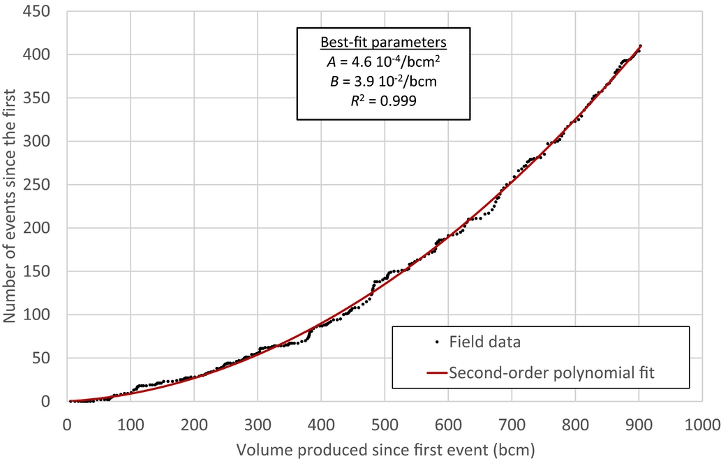
Fig. 4. The cumulative number of events (M≥1.3) versus the cumulative volume produced since the first event, together with the second-order polynomial fit starting at zero.
Note that we forced the model through a zero point defined by the first event, requiring that N=1 at V=V1. As a result, the model has only two empirical parameters. In the case of the Groningen field the first event was registered on 5 December 1991, when the cumulative production was 1272bcm. Figure 4 shows the results, including the values of the empirical parameters A and B, as derived in the Appendix.
Although the correlation coefficient of the cumulative analysis is very high, this does not necessarily prove a high goodness of fit or the ability to use this relationship as a predictive model. Besides, the cumulative relationship does not account for the differences between the model and the data observed for instance at points of 380, 500 and 650bcm of production, shown in Figure 4. A better method to honour these differences in detail is to analyse the ratio of the activity rate over the production rate as a function of the independent variable, the produced volume. The model relationship is derived in the Appendix, eqn A4. An additional advantage is that the dependent parameter (now the ratio of activity rate over productivity rate) becomes linear dependent on the cumulative produced volume since the first event. The results are shown in Figure 5. Note that we have chosen to start the model at 1 December 1991, in order to include the very first registered event. Therefore, the years analysed represent yearly periods running from 1 December of the previous year to 30 November of the year shown (see labels in Fig. 5). We also performed the analysis for a minimum magnitude of M=1.5. The results are shown in Figure 6, together with the regression analysis parameters. The goodness-of-fit for the activity rate for M≥1.3 is shown in Figure 7, and the same results for M≥1.5 are shown in Figure 8. The figures show the main statistical parameters: the standard error of prognosis, the confidence interval and the correlation coefficient.

Fig. 5. The ratio of activity rate over production rate versus the volume produced for M≥1.3, including the results from the regression analysis.
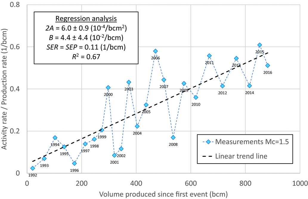
Fig. 6. The ratio of activity rate over production rate versus the volume produced for M≥1.5, including the results from the regression analysis.
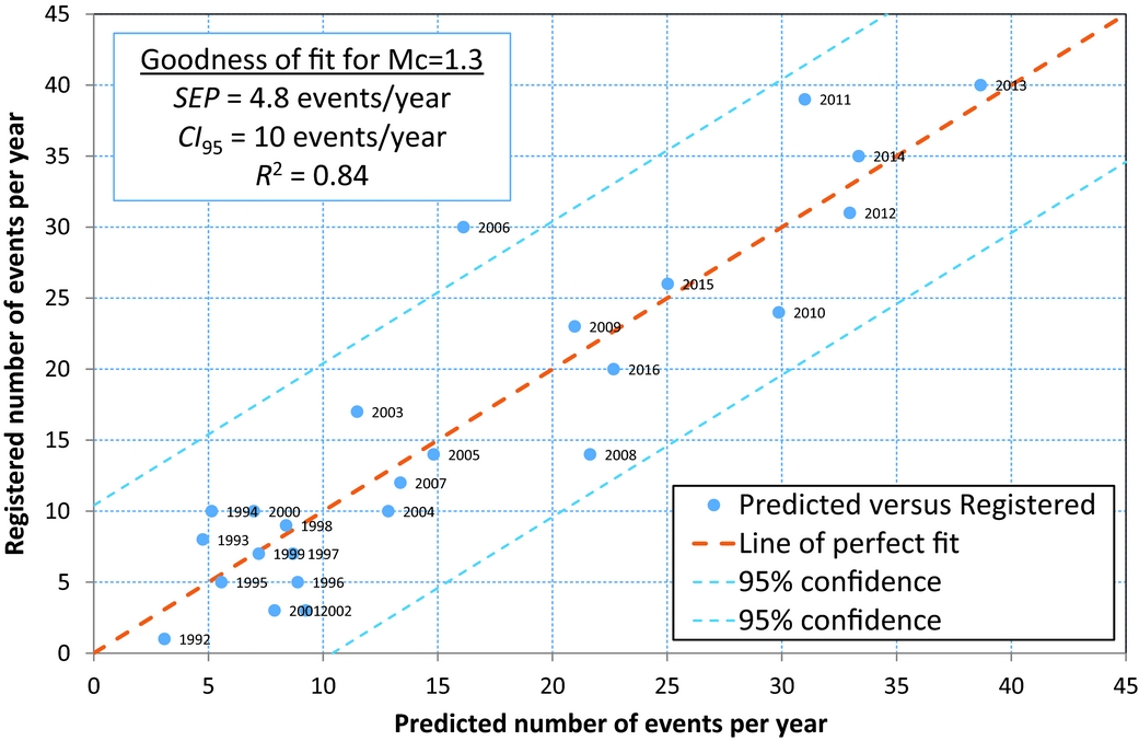
Fig. 7. Goodness of fit for the predicted activity rates per year, for M≥1.3.
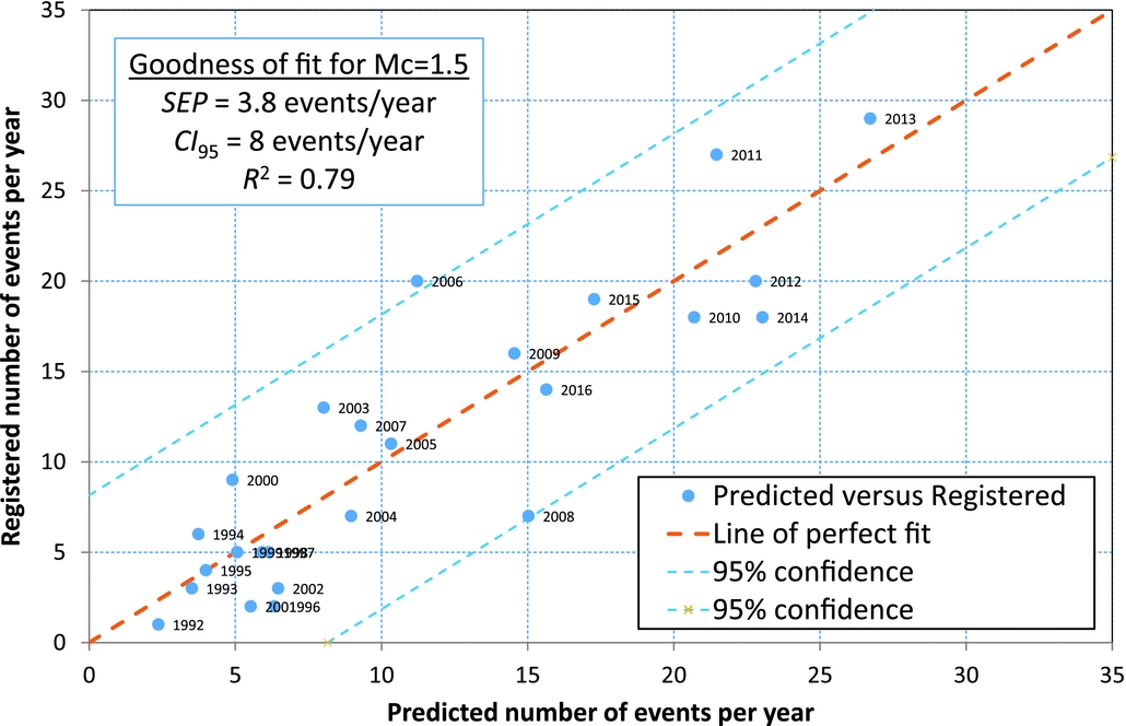
Fig. 8. Goodness of fit for the predicted activity rates per year, for M≥1.5.
Application to predictions of the activity rate
The empirical model described in the Appendix can be used to predict the number of earthquakes above a certain magnitude threshold assuming a certain amount of gas production. The empirical relationship derived from historical earthquake data can only be applied to predictions under strict assumptions. From a mathematical point of view, the predictive model with its confidence interval can at best be applied as long as the production strategy does not vary outside the range of historical production the empirical model was based upon. However, this is only true if the chosen independent variables (volume and production rate) are the only controlling variables.
The NAM (2016c) report presented a prediction of activity rate for the year 2016 for the production scenario of 27bcm in that year and considering events with magnitudes M ≥ 1.5. That prediction was made using the Extended Activity Rate model (Bourne et al., Reference Bourne and Oates2015b) which uses a probabilistic relationship to relate the compaction with the seismic activity rate. Their expectation value for 2016 was 22 events, with a 95% confidence interval ranging from 13 to 34 (NAM 2017). When applying our model to the same seismic catalogue consisting of events until the end of 2015 (also for events with magnitudes of M≥1.5) we arrived at a forecast of 16±8 events for 2016. Figure 9 shows both these predictions in comparison to the actual realisation of 13 such events in 2016.
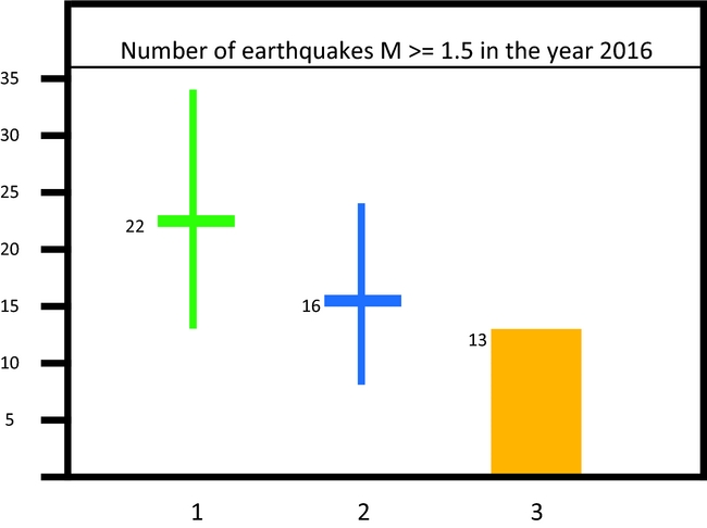
Fig. 9. A comparison of two predictions made for the activity rate for 2016, only considering earthquakes with a magnitude of M≥1.5. (1) The prognoses presented by NAM in the winningsplan (NAM, 2016c), (2) the prognoses using our empirical model described above, (3) the actual registered number of earthquakes in 2016.
From the results of the 2016 predictions, it can be concluded that both models resulted in expectation values higher than the actually recorded number of events of 13. In both cases the actual event rate lies within the 95% confidence interval of the prognoses. It seems that our empirical model does not perform worse than the model developed by NAM.
The results of the various prognoses including their confidence intervals are summarised in Table 1. We have also made prognoses for 2017, assuming a production of 24bcm for that year. The input parameters A and B for the 2017 predictions are listed in Figures 5 and 6, and the 95% confidence interval is calculated from the standard error of prediction (see Appendix), listed in Figures 7 and 8. The model predicts 14 events with a magnitude of M = 1.5 and higher and 21 events with a magnitude of M = 1.3 and higher for the year 2017.
Table 1. Prediction results for the different prognoses.

a Below the magnitude of completeness.
A potential pitfall when relating production to the number of events for such a short period (just one year) is the fact that there is probably some delay time between cause (production at the wells) and effect (earthquakes). Not all events recorded in a particular year will necessarily be the result of production in the same year. In its original cumulative form, both the effects of time delay and production fluctuation are suppressed in the analysis (Hagoort, Reference Hagoort2015). However, when the rate-ratio form was derived (see Appendix equation A4), a time window needed to be defined. One year for analysis was chosen to suppress shorter-term time delays and fluctuations. It is highly possible that the model would gain confidence if the effects of the time-delay and production fluctuations were incorporated in a causal manner, i.e. relate the cause (the production rate and its fluctuations at the well) with the consequence (seismicity caused by changes on the critical stressed faults). The next section discusses the effects of time delay.
Possible impact of delay between production and effects from production
Various researchers have analysed the delay time between changes in production volumes at the production clusters and the moment these changes have an effect elsewhere in the field, leading to seismic events (e.g. Bierman et al., 2015; Van Thienen-Visser et al., Reference Van Thienen-Visser, Sijacic, Nepveu, Van Wees and Hettelaar2015; Nepveu et al., Reference Nepveu, van Thienen-Visser and Sijacic2016; Pijpers, 2016). A reason for the fact that no strong correlation can be found could be that the delay may be varying in space and time, due to decreasing reservoir pressure.
The impact of production on the reservoir pressure can best be described with pressure transient equations (Hagoort, Reference Hagoort1988). A useful derived quantity is hydraulic diffusivity, which indicates how pressure diffusion occurs over an area in a reservoir as a result of production from a well or cluster (equation 1). Related to that is the diffusion time (or semi-steady-state time) which is given in equation 2. This is the time at which a production-induced pulse from the well arrives at a reservoir boundary. This approach has also been used by Hettema et al. (Reference Hettema, Papamichos and Schutjens2002).
 $$\begin{equation}
{D_{\rm{h}}} = \ \frac{k}{{\phi \mu {c_{\rm{t}}}}}
\end{equation}$$
$$\begin{equation}
{D_{\rm{h}}} = \ \frac{k}{{\phi \mu {c_{\rm{t}}}}}
\end{equation}$$
 $$\begin{equation}
{t_{{\rm{sss}}}}\ \; = \;\ \frac{{{r^2}}}{{4{D_{\rm{h}}}}}
\end{equation}$$
$$\begin{equation}
{t_{{\rm{sss}}}}\ \; = \;\ \frac{{{r^2}}}{{4{D_{\rm{h}}}}}
\end{equation}$$
In which:
As a first-order approach, average properties are used for the Groningen reservoir (i.e. a porosity of 16% and a permeability of 120mD). The distance between individual production clusters and the distance between clusters and faults vary strongly. Therefore we assume a range of 1–5km in our calculations. The calculations are done by varying the reservoir pressure as shown in Table 2. For a distance of 3000m at initial reservoir pressure (347bar), only 15 days are needed for a pressure signal to travel from the wellbore. However when the field is further depleted the diffusion time of the pressure signal increases significantly. At present pressure range (~70–95bar) this diffusion time has already increased to approximately 50 days. Ultimately diffusion of a signal will take about 388 days at 10bar reservoir pressure. Since the relation is quadratic, this effect becomes even more pronounced for larger distances. Figure 10 shows that, especially within the pressure range between 75 and 10bar, i.e. in the coming decade(s), pressure diffusion will become much slower.
Table 2. Development of diffusivity and diffusion time for a pressure signal with decreasing reservoir pressure at average Groningen reservoir parameters.
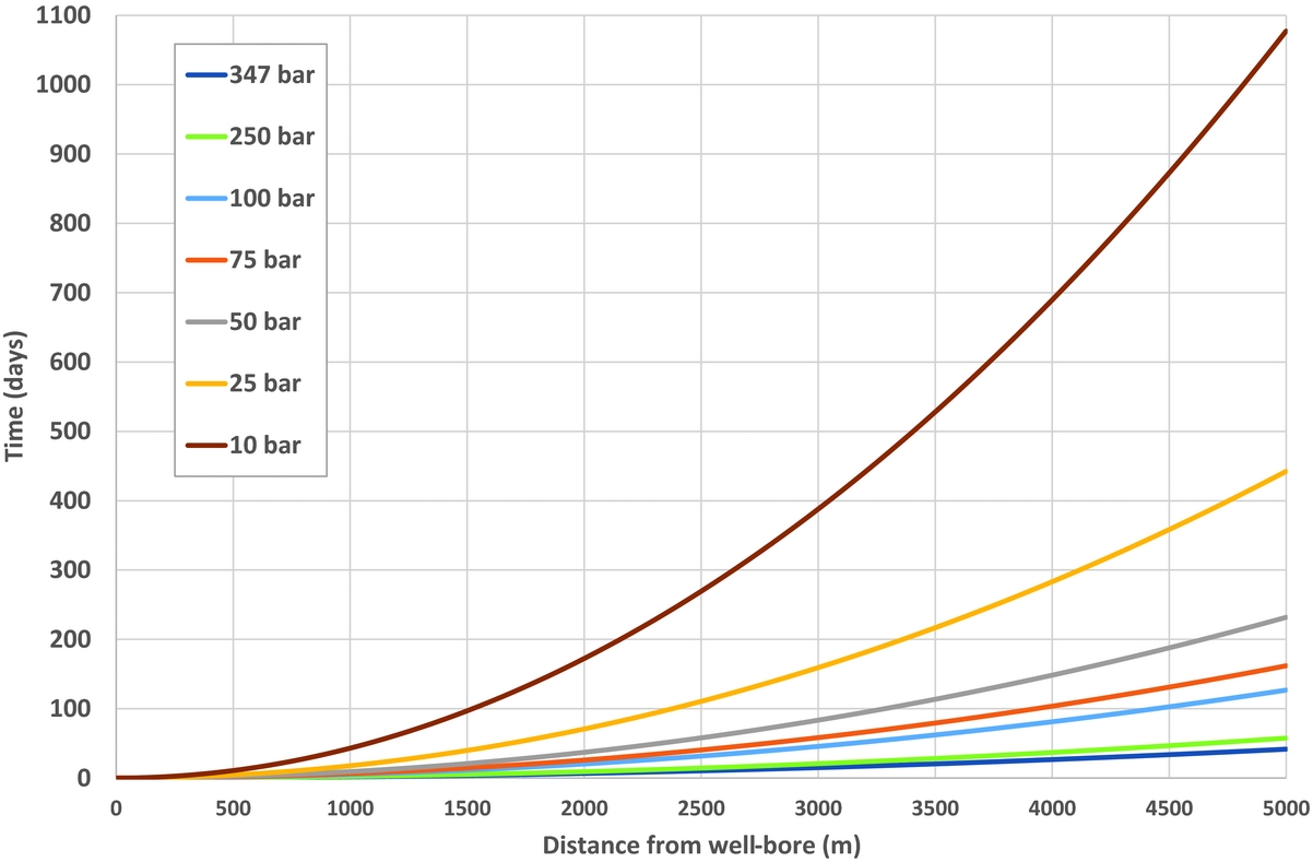
Fig. 10. The development of the time to diffuse a pressure signal through the reservoir with decreasing reservoir pressure.
The main conclusion from this section is that the time for a pressure signal to diffuse in the reservoir increases rapidly as the reservoir becomes further depleted with time. The impact is that this could have an effect on the interpretation of all models based on empirical data, especially when time dependency is considered.
Discussion
Even though the mechanisms causing the seismicity in the Groningen field are not yet fully understood, the process of induced seismicity starts with the decrease of pore pressure in the reservoir due to the production of gas. At the start of production in 1963, average reservoir pressure was 347bar. It took a decrease to about 180bar before the first seismic event was detected in 1991. This observation suggests that absolute reservoir pressure is one of the factors determining the occurrence of earthquakes. The empirical quadratic relationship found between the produced volume and the cumulative number of events leads to the conclusion that the activity rate per unit of volume produced has steadily increased. Figure 5 suggests that a few years from now a level of about one event (M≥1.3) per bcm produced would be reached. This general increase can be interpreted as the subsurface of the Groningen field becoming more sensitive to stress changes induced by production.
According to Hagoort (Reference Hagoort2015), the eventual cumulative number of events at the end of production would be a fixed number and lowering the annual production would only postpone earthquakes. The metaphor of the ‘frame rate’ effect is often used. One can play the movie slower or faster, but the cumulative number of events at the end of depletion would be fixed regardless of the way in which the field is depleted. This idea assumes that the cumulative empirical relationship described above remains the same in the future. It has, however, been suggested by others (Muntendam-Bos & de Waal, 2013) that producing the field in a way that results in lower stress rates might mean that the amount of energy released in seismogenic processes would be lower (given the same production volume). In other words, they expect that lowering the annual production volume not only results in a lower annual number of events because of the ‘frame rate’ effect, but also in an additional reduction of that number.
Considering the possibilities of producing the field in a way that is associated with a slower decrease of reservoir pressure, a second measure has been taken: taking away, or at least strongly reducing, the seasonal fluctuations in production. The idea is that this would result in reducing the high seasonal decrease of local pore pressure at the start of each winter. Nepveu et al. (Reference Nepveu, van Thienen-Visser and Sijacic2016) and Pijpers (2016) claim to have demonstrated that the seasonal fluctuations in production must have played a role in the occurrence of earthquakes. If so, future production without significant seasonal fluctuations would result in a lower seismic activity rate. There is still a lot of debate about both these notions. If this is true, the predictive power of empirical models would gain confidence if these seasonal fluctuations are causally included in the model.
The measures taken by the minister in 2016 will result in a lower (24bcma−1) annual production volume than realised since 2000 and in small seasonal fluctuation only. If this adapted manner of producing the field can be maintained for a number of years we may expect that the observed seismic activity rate in the next few years will decrease. Considering the above, it is worth investigating whether an extension of our empirical model taking into account the seasonal fluctuations would result in new insights.
Extension of the model with delay time
Our theoretical analysis shows that the delay time between production and seismic activity varies throughout the field and throughout production history (see Fig. 10). Application of these model results in an activity rate model that requires a space- and time-dependent delay time. Inclusion of this effect in seismological models may increase the predictive power of these models. A varying delay time is a relevant extension to build into our empirical model.
Application of the model to sub-regions of the field
In a situation where the Groningen field would consist of a number of completely sealed-off blocks, these blocks would be expected to each show empirical relationships very similar to the Groningen field-wide relationship derived in this paper. In order to test the applicability we divided the Groningen field into regions along bounding faults.
There are, however, some difficulties with this. Some parts of the field show too low an activity rate to do robust statistical analysis on. Furthermore, the division of the field can be done in various ways. In our exercise we chose to use the boundaries of areas with the same initial free water level (NAM, 2016b). These boundaries could be considered somewhat arbitrary because the number of data points for initial free water level is low and because of the large number of faults which may act as barriers and boundaries to flow between regions. However, there are uncertainties associated with the transmissibility of these faults leading to multiple scenarios that could be chosen to divide the field for empirical analysis on parts of the field. Finally, there is the uncertainty with which the locations of the epicentres have been determined. We allocated events to specific sub-regions, but in reality events close to a boundary fault may have been the result of production from the neighbouring block. Figure 11 shows the resulting plots of cumulative number of events vs the cumulative volume of production for different regions.
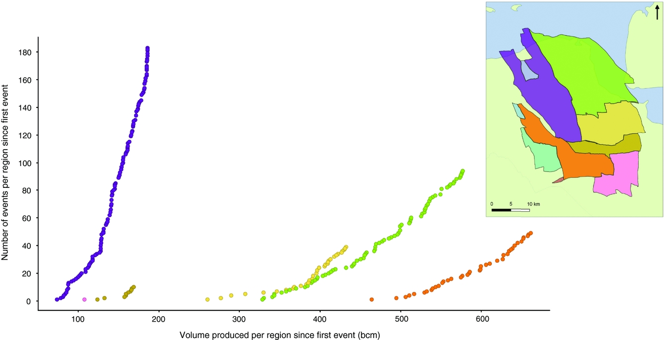
Fig. 11. The cumulative number of events (M≥1.3) per region since the first event versus the cumulative volume produced per region since the first event. Colours of the curves equal the colours of regions in the map. Note that each graph has a different (average) reservoir pressure as the starting point.
This is the first step in investigating the challenges related to analysing the model performance after dividing the field into regions. The graphs for different regions differ to some extent, showing clear differences in steepness. These clear differences should be analysed further. Note that each graph has a different (average) reservoir pressure as the starting point, which may partially explain the differences. Differences in reservoir properties, fault density and characteristics and production history may contribute to the observed differences. Empirical relationships for parts of the field will be analysed for alternative divisions, taking into account these faults which are barriers or boundaries to gas flow. Comparing the goodness of fits for the various regions based on an alternative division may yield additional support to decisions on changes in production strategy at regional level.
Conclusions
In this paper we started from an empirical relationship between the cumulative number of seismic events and cumulative gas production in the Groningen field. We demonstrated that a better way to analyse the data, determine the model parameters and their uncertainty and make predictions with their confidence intervals is to analyse the ratio of activity rate over production rate versus the cumulative production. The model predicts that the ratio of activity rate over production rate will increase linear with produced volume. We performed a regression analysis based on all events with a magnitude of 1.3 and larger, because we consider this value to be the magnitude of completeness. We have also performed a regression analysis based on events with a magnitude of 1.5 and larger, because we compared our forecast with forecasts performed by others. Our prognosis for 2016 (using only events recorded before 2016) gave a prediction of 16±8 events for M≥1.5. By the end of 2016, 13 such events had been recorded. The forecast using this empirical relationship performed no worse than other forecasts.
It is realised that, when relating the number of recorded seismic events within a specific period (of one year) to the amount of gas production in the same period, the possible time delay between cause (production) and effect (earthquakes) would weaken the confidence of the model predictions. Basic gas reservoir theory shows that the contribution to that delay is the result from the time needed for pressure diffusion through the reservoir, which varies both in space and time. There is also a systematic increase of delay times with decreasing reservoir pressure.
Future work can be done to include the delay time effect and the production fluctuations in the empirical model. Also, more work could be done to study the applicability of the model to the various sub-regions of the Groningen field. Such a more detailed analysis would benefit from a more accurate determination of the location of the hypocentres than has been available until recently.
Acknowledgements
We thank Marloes Kortekaas, Raymond Godderij, Thijs Huijskes and two anonymous reviewers for their valuable comments.
Appendix: An empirical model for the seismic activity rate
The history of the seismic events of the Groningen field suggests the following empirical relationship between the cumulative number of events and the cumulative volume produced:
 $$\begin{equation}
N = A{\left( {{V_p} - {V_1}} \right)^2} + B\left( {{V_p} - {V_1}} \right) + {\rm{1 }}\left({{\rm{for }} \ {V_p} \ge {V_1}} \right)
\end{equation}$$
$$\begin{equation}
N = A{\left( {{V_p} - {V_1}} \right)^2} + B\left( {{V_p} - {V_1}} \right) + {\rm{1 }}\left({{\rm{for }} \ {V_p} \ge {V_1}} \right)
\end{equation}$$
where
 $$\begin{equation*}
\begin{array}{@{}l@{}} N = {\rm{Cumulative\ number\ of\ events\ for\ M}} \ge {\rm{1}}{\rm{.3}}\\ {V_p} = {\rm{Cumulative\ gas\ volume\ produced\ (bcm)}}\\ {V_1} = {\rm{ Cumulative\ gas\ volume\ produced\ at\ the\ first\ event\ (bcm)}}\\ A = {\rm{Empirical\ constant }}\left( {{{\rm{1}}
/ {{\rm{bc}}{{\rm{m}}^{\rm{2}}}}}} \right)\\ B = {\rm{ Empirical\ constant }}\left( {{{\rm{1}}
/ {{\rm{bcm}}}}} \right) \end{array}
\end{equation*}$$
$$\begin{equation*}
\begin{array}{@{}l@{}} N = {\rm{Cumulative\ number\ of\ events\ for\ M}} \ge {\rm{1}}{\rm{.3}}\\ {V_p} = {\rm{Cumulative\ gas\ volume\ produced\ (bcm)}}\\ {V_1} = {\rm{ Cumulative\ gas\ volume\ produced\ at\ the\ first\ event\ (bcm)}}\\ A = {\rm{Empirical\ constant }}\left( {{{\rm{1}}
/ {{\rm{bc}}{{\rm{m}}^{\rm{2}}}}}} \right)\\ B = {\rm{ Empirical\ constant }}\left( {{{\rm{1}}
/ {{\rm{bcm}}}}} \right) \end{array}
\end{equation*}$$
Since there are yearly seasonal production rate fluctuations and possible time delays between production and seismicity, we choose a yearly time window for analysis:
 $$\begin{equation}
\Delta {V_p} = {V_{p + 1}} - {V_p}
\end{equation}$$
$$\begin{equation}
\Delta {V_p} = {V_{p + 1}} - {V_p}
\end{equation}$$
By applying this definition to the model, eqn A1 gives after rearranging:
 $$\begin{equation}
\Delta N = A\left[ {2\left( {{V_{p + 1}} - {V_1}} \right)\Delta {V_p} - {{\left( {\Delta {V_p}} \right)}^2}} \right] + B\Delta {V_p}
\end{equation}$$
$$\begin{equation}
\Delta N = A\left[ {2\left( {{V_{p + 1}} - {V_1}} \right)\Delta {V_p} - {{\left( {\Delta {V_p}} \right)}^2}} \right] + B\Delta {V_p}
\end{equation}$$
Now the ratio of seismic activity rate over the production rate can be written as (applying eqn A2):
 $$\begin{equation}
\frac{{\Delta N}}{{\Delta {V_p}}} = \frac{{\frac{{\Delta N}}{{\Delta t}}}}{{\frac{{\Delta {V_p}}}{{\Delta t}}}} = \frac{\rm{AR}}{\rm{PR}} = 2A\left[ {\left( {{V_p} - {V_1}} \right) + \frac{{\Delta {V_p}}}{2}} \right] + B
\end{equation}$$
$$\begin{equation}
\frac{{\Delta N}}{{\Delta {V_p}}} = \frac{{\frac{{\Delta N}}{{\Delta t}}}}{{\frac{{\Delta {V_p}}}{{\Delta t}}}} = \frac{\rm{AR}}{\rm{PR}} = 2A\left[ {\left( {{V_p} - {V_1}} \right) + \frac{{\Delta {V_p}}}{2}} \right] + B
\end{equation}$$
Here AR is the seismic activity rate (number of events per year) and PR is the production rate (number of bcm produced per year). This rate-ratio is considered to be the best way to analyse the data, its model parameters and the variation. For prognosis of the yearly production volume, the relationship becomes:
 $$\begin{equation}
{\rm {AR}} = \left[ {2A\left( {\left( {{V_p} - {V_1}} \right) + \frac{{\Delta {V_p}}}{2}} \right) + B} \right]{\rm {PR}}
\end{equation}$$
$$\begin{equation}
{\rm {AR}} = \left[ {2A\left( {\left( {{V_p} - {V_1}} \right) + \frac{{\Delta {V_p}}}{2}} \right) + B} \right]{\rm {PR}}
\end{equation}$$
Relationship (A4) can also be used directly for historical data analysis. Relationship (A5) can also be inverted to determine the production rate leading to a certain activity rate:
 $$\begin{equation}
{\rm {PR}} = \frac{\rm{AR}}{{2A\left[ {\left( {{V_p} - {V_1}} \right) + \frac{{\Delta {V_p}}}{2}} \right] + B}}
\end{equation}$$
$$\begin{equation}
{\rm {PR}} = \frac{\rm{AR}}{{2A\left[ {\left( {{V_p} - {V_1}} \right) + \frac{{\Delta {V_p}}}{2}} \right] + B}}
\end{equation}$$
When comparing the data with the model, it is useful to apply the standard error of residuals (SER), defined as the root of the mean of the squares of the differences between the registered and predicted events (Levine et al., Reference Levine, Ramsey and Smidt2001):
 $$\begin{equation}
{\rm {SER}} = \sqrt {\frac{1}{{n - 2}}\sum\limits_{i = 1}^n {{{\left( {{y_{i,{\rm{meas}}}} - {y_{i,{\rm{model}}}}} \right)}^2}} }
\end{equation}$$
$$\begin{equation}
{\rm {SER}} = \sqrt {\frac{1}{{n - 2}}\sum\limits_{i = 1}^n {{{\left( {{y_{i,{\rm{meas}}}} - {y_{i,{\rm{model}}}}} \right)}^2}} }
\end{equation}$$
Here n is the number of observations, 25 years in this case. For the ‘goodness of fit’ analysis, we apply the standard error of prediction, defined as:
 $$\begin{equation}
{\rm {SEP}} = \sqrt {\frac{1}{{n - 2}}\left[ {\sum\limits_{i = 1}^n {{{\left( {{y_i} - \overline y } \right)}^2}} - \frac{{{{\left( {\sum\limits_{i = 1}^n {\left( {{x_i} - \overline x } \right)\left( {{y_i} - \overline y } \right)} } \right)}^2}}}{{\sum\limits_{i = 1}^n {{{\left( {{x_i} - \overline x } \right)}^2}} }}} \right]}
\end{equation}$$
$$\begin{equation}
{\rm {SEP}} = \sqrt {\frac{1}{{n - 2}}\left[ {\sum\limits_{i = 1}^n {{{\left( {{y_i} - \overline y } \right)}^2}} - \frac{{{{\left( {\sum\limits_{i = 1}^n {\left( {{x_i} - \overline x } \right)\left( {{y_i} - \overline y } \right)} } \right)}^2}}}{{\sum\limits_{i = 1}^n {{{\left( {{x_i} - \overline x } \right)}^2}} }}} \right]}
\end{equation}$$
From both these parameters the confidence interval can be determined. To evaluate if the deviation between the model prediction and the historical registered events is normally distributed, a cumulative normal probability plot is created (Levine et al., Reference Levine, Ramsey and Smidt2001, §5.5). The parameters are the normalised Z-value and the cumulative probability of observation i, defined by:
 $$\begin{equation}
\begin{array}{@{}c@{}} {Z_i} = \frac{{{y_{{\rm{registered}}}} - {y_{{\rm{predicted}}}}}}{{SD}}\\[4pt] {p_i} = \frac{{i - 0.5}}{n} \end{array}
\end{equation}$$
$$\begin{equation}
\begin{array}{@{}c@{}} {Z_i} = \frac{{{y_{{\rm{registered}}}} - {y_{{\rm{predicted}}}}}}{{SD}}\\[4pt] {p_i} = \frac{{i - 0.5}}{n} \end{array}
\end{equation}$$
The results shown in Figure 12 demonstrate that the model to data deviation is roughly normally distributed. Both SER and SEP can be used to estimate the deviation of a single event. For a 95% confidence interval, based on 25 data points (23 degrees of freedom), the critical confidence t-factor is 2.07 (Levine et al., Reference Levine, Ramsey and Smidt2001, table A.4). The 95% confidence interval for a single event becomes (Levine et al., Reference Levine, Ramsey and Smidt2001, §12.8):
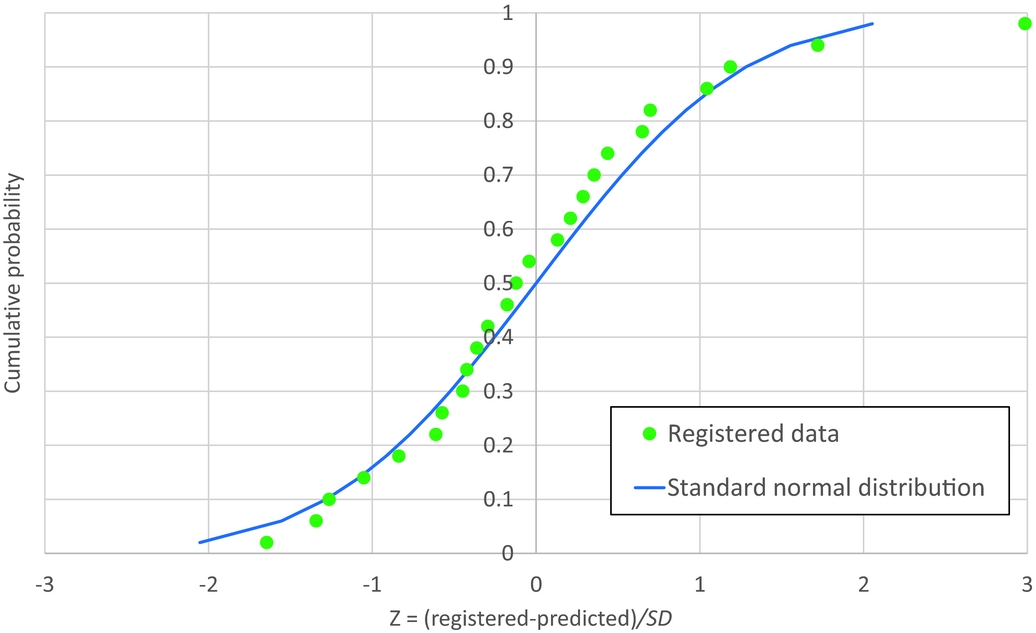
Fig. 12. The normal probability plot, showing the cumulative probability versus the Z parameter for the registered data and the corresponding standard normal distribution.
 $$\begin{eqnarray}
{\rm {CI}}_{95} &=& {t_{n - 2}} \cdot {\rm {SEP}} \cdot \sqrt {1 + {h_i}} = 2.07 \cdot {\rm {SEP}}\nonumber\\
&& \cdot\, \sqrt {1 + \frac{1}{n} + \frac{{{{\left( {{x_i} - \overline x } \right)}^2}}}{{\sum\limits_{i = 1}^n {{{\left( {{x_i} - \overline x } \right)}^2}} }}} \approx 2.15 \cdot {\rm {SEP}}
\end{eqnarray}$$
$$\begin{eqnarray}
{\rm {CI}}_{95} &=& {t_{n - 2}} \cdot {\rm {SEP}} \cdot \sqrt {1 + {h_i}} = 2.07 \cdot {\rm {SEP}}\nonumber\\
&& \cdot\, \sqrt {1 + \frac{1}{n} + \frac{{{{\left( {{x_i} - \overline x } \right)}^2}}}{{\sum\limits_{i = 1}^n {{{\left( {{x_i} - \overline x } \right)}^2}} }}} \approx 2.15 \cdot {\rm {SEP}}
\end{eqnarray}$$


 Open access