

Introduction and background
Gas production from the Groningen field induces seismicity that in recent years has started to cause concerns about the future strength of earthquake ground motions and the resilience of existing buildings to these ground motions. Ongoing gas production is depleting the pressure of hydrocarbon gas within the reservoir pore space causing the reservoir to compact. In turn, reservoir compaction increases the mechanical loads acting on pre-existing geological faults within and close to the reservoir. Some small fraction of these faults become unstable and are therefore prone to slip. Abrupt slip on such a fault results in an earthquake that radiates seismic energy.
The established method for assessing the future likelihood of ground motion events is Probabilistic Seismic Hazard Assessment (PSHA) (e.g. Cornell, Reference Cornell1968; McGuire, Reference McGuire2008). The two essential elements of PSHA are a seismological model to describe the probability distribution of possible future earthquake locations and magnitudes, and a ground motion model to describe the probability distribution of ground motions, such as peak ground accelerations, at a given distance from an earthquake of a given magnitude. The combination of these two elements yields an estimate for the probability distribution of future ground motion events at a site of interest. Extension of the methods of PSHA to also encompass assessment of the risk of building damage or injury due to earthquake ground motions can be termed Probabilistic Seismic Hazard and Risk Assessment (PSHRA). This is an extension of PSHA that further combines the seismic hazard models with the probability of building damage for a given ground motion event and the probability of injury for a given building damage event.
The first step in PSHRA is the development of a seismological model which summarises the statistics of the spatial and temporal distributions of seismicity in an identified source zone and so enables us to forecast event locations, origin times and magnitudes. Classical approaches often use blocked models of source regions (van Eck et al., Reference van Eck, Goutbeek, Haak and Dost2006) with seismic activity levels given by assumed Gutenberg–Richter (or other) frequency–magnitude distributions derived from existing earthquake catalogues. An approach of this kind was applied by KNMI in their earlier work on the application of PSHA to the North Netherlands gas fields (van Eck et al., Reference van Eck, Goutbeek, Haak and Dost2006). It is however recognised that seismicity induced over the Groningen field is driven by reservoir strains and pore pressure depletion due to the gas production: this gives the possibility of constructing a statistical geomechanical model of the seismicity based on the spatially and temporally varying pattern of production. Here we discuss how a range of such seismological models for Groningen have been built and calibrated (history-matched) against field observations and subsequently used to forecast induced seismicity as the basis of our Monte Carlo PSHRA methodology (Bourne et al., Reference Bourne, Oates, van Elk and Doornhof2014, Reference Bourne, Oates, Bommer, Dost, van Elk and Doornhof2015). An alternative, explicit fault-model-based, approach is discussed by Lele et al. (Reference Lele, Hsu, Garzon, DeDontney, Searles, Gist, Sanz, Biediger and Dale2016).
Seismic moment rate model dependent on reservoir shear strains
The first version of this seismological model (Bourne et al. Reference Bourne, Oates, van Elk and Doornhof2014) was founded on the observation that seismicity over the field correlates well with mapped reservoir compaction obtained from the inversion of surface geodetic data (see Figs 1 and 2 and Bierman et al., Reference Bierman, Kraaijeveld and Bourne2015). The fundamental geomechanical work of Kostrov (Reference Kostrov1974) and McGarr (Reference McGarr1976), which shows how volume change can be connected to the summed moments of the induced fault slip, was used to relate the moment budget of the induced seismicity to the reservoir strain. Specifically, for a population of N earthquakes within a volume, V, the average incremental strain due to seismic slip on faults is
 $$\begin{equation*}
{\bar{\epsilon }_{ij}} = \frac{1}{{2\mu V}}\mathop \sum \limits_{k = 1}^N {\mathfrak{M}^k}\mathfrak{m}_{ij}^k
\end{equation*}$$
$$\begin{equation*}
{\bar{\epsilon }_{ij}} = \frac{1}{{2\mu V}}\mathop \sum \limits_{k = 1}^N {\mathfrak{M}^k}\mathfrak{m}_{ij}^k
\end{equation*}$$
where ${\mathfrak{M}^k}$
and
${\mathfrak{M}^k}$
and $\mathfrak{m}_{ij}^k$
are the seismic moment and unit moment tensor of the kth event respectively and μ is the shear modulus of the rock. The maximum seismic moment,
$\mathfrak{m}_{ij}^k$
are the seismic moment and unit moment tensor of the kth event respectively and μ is the shear modulus of the rock. The maximum seismic moment, ${\mathfrak{M}_{{\rm{max}}}}$
, due to a bulk reservoir volume change ΔV is given by Bourne et al. (Reference Bourne, Oates, van Elk and Doornhof2014) as
${\mathfrak{M}_{{\rm{max}}}}$
, due to a bulk reservoir volume change ΔV is given by Bourne et al. (Reference Bourne, Oates, van Elk and Doornhof2014) as
 $$\begin{equation*}
{\mathfrak{M}_{{\rm{max}}}} = \frac{4}{3}\mu \left| {\Delta V} \right|
\end{equation*}$$
$$\begin{equation*}
{\mathfrak{M}_{{\rm{max}}}} = \frac{4}{3}\mu \left| {\Delta V} \right|
\end{equation*}$$
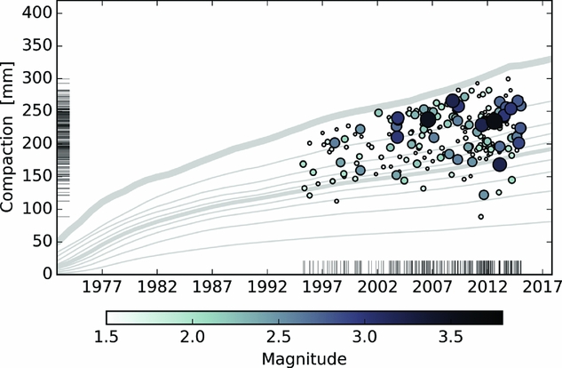
Fig. 1. Time series of the occurrence of ML≥1.5 Groningen earthquakes versus reservoir compaction at the origin time and map location of each event.

Fig. 2. Plots of (A) the number density of observed epicentres of ML≥1.5 earthquakes and (B) the same epicentres shown in relation to reservoir compaction estimated by inversion of the geodetic data.
A strain partitioning function was introduced to scale the moment budget inferred from the reservoir volume change by the fraction of reservoir strain that is released by earthquakes. It is observed that only a small fraction of the available compaction strain energy has been accommodated as seismicity. The observed escalation of the field's induced seismicity with increasing compaction led to the use of a temporally and spatially varying partition function which has the form of a compaction-dependent exponential.
Activity rate model dependent on reservoir shear strains
The seismic moment rate model matched the observed seismicity, albeit within the large uncertainty range associated with total seismic moments that depend strongly on the moment of the few largest events. A more precise fit to binned compaction data was obtained with an alternative model based on an empirical stochastic relationship between the rate of earthquake nucleation and reservoir shear strains induced by reservoir compaction (Fig. 3). Similar approaches have been used to describe injection-induced seismicity (e.g. Shapiro et al., Reference Shapiro, Dinske and Langenbruch2010, Reference Shapiro, Kruger and Dinske2013; Mena et al., Reference Mena, Wiemer and Bachmann2013). In such activity rate models the event nucleation rate is given by a function, λ p, of compaction which is therefore spatially and temporally varying resulting in an inhomogeneous Poisson process defined as follows:
 $$\begin{equation*}
\Pr \left\{ {N\left( {\omega ,\omega + t} \right) = 0} \right\} = {\rm{exp}}\left( { - \mathop \int_\omega ^{\omega + t} {\lambda _{\rm{p}}}\left( u \right)du} \right)
\end{equation*}$$
$$\begin{equation*}
\Pr \left\{ {N\left( {\omega ,\omega + t} \right) = 0} \right\} = {\rm{exp}}\left( { - \mathop \int_\omega ^{\omega + t} {\lambda _{\rm{p}}}\left( u \right)du} \right)
\end{equation*}$$

Fig. 3. Plots of (A) reservoir strain thickness and epicentres (1995–2015, Mw≥1.5). (B, C) Activity rate and strain partitioning versus reservoir strain thickness.
The observed earthquake activity rate trend relative to reservoir compaction inferred from geodetic monitoring of surface displacements indicates an exponential-like trend such that the expected number of events between times t0 and ts can then be written as
 $$\begin{equation*}
{\rm{\Lambda }}\left( {{t_0}} \right) - {\rm{\Lambda }}\left( {{t_{\rm{s}}}} \right) = {\beta _0}\mathop \int_S^{} c(x,{t_0}){e^{{\beta _1}c\left( {x,{t_0}} \right)}} - c\left( {x,{t_{\rm{s}}}} \right){e^{{\beta _1}c\left( {x,{t_{\rm{s}}}} \right)}}dS
\end{equation*}$$
$$\begin{equation*}
{\rm{\Lambda }}\left( {{t_0}} \right) - {\rm{\Lambda }}\left( {{t_{\rm{s}}}} \right) = {\beta _0}\mathop \int_S^{} c(x,{t_0}){e^{{\beta _1}c\left( {x,{t_0}} \right)}} - c\left( {x,{t_{\rm{s}}}} \right){e^{{\beta _1}c\left( {x,{t_{\rm{s}}}} \right)}}dS
\end{equation*}$$
where ${\rm{\Lambda }}( t ) = \mathop \smallint _S^{} \mathop \smallint _0^t {\lambda _{\rm{p}}}( {x,t} )dSdt$
, c(x,t) is the compaction at location x and time t, β
0 and β
1 are the coefficients of the exponential trend model and S is the region of interest considered. The exponential captures the observed increase in the number of earthquakes per unit reservoir compaction with increasing reservoir compaction.
${\rm{\Lambda }}( t ) = \mathop \smallint _S^{} \mathop \smallint _0^t {\lambda _{\rm{p}}}( {x,t} )dSdt$
, c(x,t) is the compaction at location x and time t, β
0 and β
1 are the coefficients of the exponential trend model and S is the region of interest considered. The exponential captures the observed increase in the number of earthquakes per unit reservoir compaction with increasing reservoir compaction.
Activity rate model with aftershocks
The class of activity rate models admits several natural generalisations and extensions which have been found to improve the model performance. Aftershock sequences, seen as the spatial and temporal clustering of events around previous events, can be incorporated in the rate function, λ, in a natural way using the Epidemic Type After Shock (ETAS) model (Ogata, Reference Ogata1998, Reference Ogata2011). ETAS associates spatial and temporal power law decays of aftershock seismicity with parent events. Each event can be regarded as the parent of a possible aftershock sequence resulting in cascading generations of aftershocks with steadily diminishing numbers of events the statistics of which are determined by the ETAS model parameters, obtained from the catalogue data by a maximum likelihood method. The rate function λ is extended as follows:
 $$\begin{equation*}
\lambda \left( {x,t} \right) = {\lambda _{\rm{p}}} + \sum Kg\left( {{t_{\rm{e}}}} \right)h\left( {{r_{\rm{e}}}} \right){e^{a\left( {M - {M_0}} \right)}}_{}
\end{equation*}$$
$$\begin{equation*}
\lambda \left( {x,t} \right) = {\lambda _{\rm{p}}} + \sum Kg\left( {{t_{\rm{e}}}} \right)h\left( {{r_{\rm{e}}}} \right){e^{a\left( {M - {M_0}} \right)}}_{}
\end{equation*}$$
Here λ p is the rate function for independent events and the second term is the aftershock contribution where the sum is over all events – independent main shocks but also aftershocks since aftershocks can themselves be parents for further aftershock sequences. g(t e) and h(r e) are the probability density functions for temporal and spatial triggering of aftershocks, t e is the inter-event time, r e is the inter-event distance, M is the event magnitude, M 0 is the minimum magnitude, and K a constant. The ETAS and activity rate model parameter values and their confidence regions were obtained as joint maximum likelihood estimates. In our simulations it is typical for 10–20% of the total number of synthetic earthquakes to be members of aftershock sequences, and statistical testing has demonstrated the necessity of inclusion of this degree of clustering.
Activity rate model dependent on fault-controlled, reservoir shear strains
A further generalisation of the model is the incorporation of the influence of lateral topographic gradients of the compacting reservoir that localise the induced shear strains around faults that offset the reservoir formation. This means that pre-existing faults with reservoir offsets will be centres of increased seismic moment release rate relative to the background level. This allows forecast earthquakes to be concentrated on or near the major mapped faults, albeit at the cost of the introduction of an additional model parameter determining the relative importance of the background seismicity, likely associated with unmapped faults, and localised seismicity around explicit mapped faults with reservoir offsets. Results generated from the extended activity rate model including ETAS aftershocks and fault-controlled lateral topographic gradients are shown in Figures 4–6 which compare modelled activity rates with observations up until the end of 2015. In Figures 5 and 6 the left- and right-hand figures of each row of plots show two different offtake scenarios with the same total production (e.g. 21bcm and 21bcmHRA) – it can be seen that differently distributing a given production volume across the production well clusters makes very little difference to the modelled seismicity. The plots in Figure 5, which shows annual event counts, have tighter uncertainty bounds than the annual seismic moment plots of Figure 6. This is an illustration of one of the key motivations for switching from a total moment budget representation to a model based on event rates. The total moment of a seismic catalogue is dominated by the moment of the few largest events – this inevitably compounds the stochastic variation in the poorly sampled tail of the frequency–magnitude distribution, leading to greater variability for total moment budgets than for total numbers of events.

Fig. 4. Maps of expected annual event density from 1995 to 2022 according to the Activity Rate Model including ETAS aftershock components and lateral topographic gradients. The forecast is based on a 33bcma−1 production plan. Grey dots are epicentres of ML≥1.5 earthquakes.

Fig. 5. The annual number of ML≥1.5 events according to the seismological model with aftershocks for the different production scenarios (the left- and right-hand columns of figures compare different offtake scenarios with the same total production). Simulated results are based on 10,000 independent simulations; grey lines and regions denote the expected annual event count and its 95% confidence interval respectively.

Fig. 6. The annual total seismic moment according to the seismological model with aftershocks for the different production scenarios (the left- and right-hand columns of figures compare different offtake scenarios with the same total production). Simulated results are based on 10,000 independent simulations; grey lines and regions denote the expected annual total seismic moment and its 95% confidence interval respectively.
Magnitudes of the modelled earthquake occurrences are drawn from the Cornell–Vanmarcke probability distribution. This is a truncated exponential distribution characterised by a slope measured by the b-value, and an upper bound, M max, corresponding to the maximum possible magnitude. Initial work was based on b-value determinations for the entire Groningen catalogue (1 April 1995 – 31 December 2014) which were consistent with the usually accepted b-value of 1. More recently, additional calculations have been carried out to ascertain whether spatially varying b-values could be reliably determined from the available data. Although the catalogue is too sparse for accepted b-value mapping methods (Wiemer, Reference Wiemer2001; Wiemer & Wyss, Reference Wiemer and Wyss2002), significantly different b-values were found for regions of 5km radius centred on Loppersum and Ten Boer, the b-value for Loppersum being significantly lower than the value of 0.966 found for the catalogue as a whole. Despite these indications of a spatially varying b-value there are no clear indications of any systematic dependence of the b-value on time or event rate (Harris & Bourne Reference Harris and Bourne2015).
A single estimate of M max=6.4 for induced seismicity is obtained from the expected total bulk reservoir volume change (Bourne et al., Reference Bourne, Oates, van Elk and Doornhof2014). A range of maximum magnitudes for induced and triggered seismicity was subsequently proposed by drawing on a broader range of site-specific and global analogue data and expert engineering judgement (NAM, 2016).
Discussion and conclusions
A range of alternative seismological models have been developed to support site-specific Probabilistic Seismic Hazard and Risk assessment for the Groningen field. Each model provides the capability to make a short-term forecast for the probability density functions that describe event numbers, event locations, event occurrence times, and event magnitudes as a function of a range of alternative future gas production plans. These models are all conditioned on the observed seismicity and its covariation with reservoir strains. This choice is motivated by following the physical process of earthquakes accommodating strains and the availability of comprehensive geodetic monitoring of surface displacements that measure the spatial–temporal distribution of strains within the Groningen reservoir throughout its entire production history.
Common to all models is the observed exponential-like trend in seismic moment rates and activity rates relative to reservoir strain. The physical basis for this is the progressive failure of a heterogeneous fault population where an increasingly large fraction of these fault systems becomes seismically active under the steadily increasing mechanical loads induced by the cumulative gas production and associated pore pressure depletion. This exponential-like trend is required to match the observed progressive rise in activity rates and seismic moment rates relative to the history of gas production.
The inclusion of aftershocks in the seismological model via the ETAS model is also essential to account for the observed significant spatial and temporal clustering of events in excess of that expected for independent events. This also reproduces the observed coupling between event magnitudes and activity rates that is responsible for larger aleatory variations in activity rates than would be expected for independent events. Finally, the inclusion of structural heterogeneity via fault-controlled strain localisation associated with fault throws mapped from the reflection seismic image further improves the spatial consistency between the observed and modelled seismicity. This current seismological model combines geomechanical knowledge of reservoir deformation processes with statistical inference to describe the earthquake process. Despite few degrees of freedom, this model matches past seismicity within appropriate confidence limits and limited bias. Nonetheless, the development history of these models to date leads us to anticipate the need for further adaptations in response to yet further complexity revealed by the ongoing geophysical and geodetic monitoring (see Bierman et al., Reference Bierman, Kraaijeveld and Bourne2015).
Appendix – List of mathematical symbols used


 Open access