


1 Introduction
Large-scale information networks are becoming ubiquitous. Mining knowledge from these information networks proves useful in a broad range of applications. For various analysis and prediction tasks on networks, representation of networks in a hyperspace enables effective use of out-of-the-shelf machine learning algorithms. In recent years, node embeddings have gained popularity in network representation (Goyal & Ferrara, Reference Goyal and Ferrara2018).
Node embeddings aim to map each node in the network to a low-dimensional vector representation to extract features that represent the topological characteristics of the network. Many techniques are developed for this purpose (Grover & Leskovec, Reference Grover and Leskovec2016; Ahmed et al., Reference Ahmed, Rossi, Lee, Willke, Zhou, Kong and Eldardiry2019; Tang et al., Reference Tang, Qu, Wang, Zhang, Yan and Mei2015), and these techniques are shown to be effective in addressing problems such as link prediction (Yue et al., Reference Yue, Wang, Huang, Parthasarathy, Moosavinasab and Huang2020; Kuo et al., Reference Kuo, Yan, Huang, Kung and Lin2013), node classification (Cavallari et al., Reference Cavallari, Zheng, Cai, Chang and Cambria2017), and clustering (Rozemberczki et al., Reference Rozemberczki, Davies, Sarkar and Sutton2019).
Many real-life networks are versioned (Cowman et al., Reference Cowman, Co?kun, Grama and Koyutürk2020) or multiplex (Park et al., Reference Park, Kim, Han and Yu2020). Different versions of a network have the same set of nodes and different sets of edges. These different sets of edges may represent identical semantics but different sources (e.g., protein–protein interaction (PPI) networks obtained from different databases) or different semantics (e.g., physical PPIs vs. genetic interactions). Consensus embedding, a concept we introduced recently (Li & Koyutürk, Reference Li and Koyutürk2020), aims to compute node embeddings for the integration of multiple network versions using the embeddings obtained from the individual versions. To compute consensus embeddings, we proposed two dimensionality reduction methods: singular value decomposition (SVD) and Variational Autoencoder. We showed that the link prediction accuracy of consensus embeddings is close to the accuracy provided by embeddings computed directly from the integrated network. We also showed that consensus embedding can improve the efficiency of processing combinatorial link prediction queries, and balances the trade-off between the earnings in query runtime and pre-processing time.
In this paper, we extend the framework for computing consensus embeddings. First, we generalize the notion of consensus embeddings such that the number of dimensions in the embedding of different individual networks can be different. Observing that these embeddings represent different hyperspaces, we adapt a well-established statistical method for mapping two spaces to each other, namely Canonical Correlation Analysis (CCA) (Hotelling, Reference Hotelling1936), to compute consensus embeddings. For computing consensus embeddings of multiple network versions, we apply Generalized Canonical Correlation Analysis (GCCA) (Kettenring et al., 1971).
Since versioned networks have identical node sets and their edge sets can overlap significantly, it can be expected that the embedding spaces of different versions can be similar. Indeed, state-of-the-art machine learning applications use simple aggregation to integrate embeddings of multiplex networks (Park et al., Reference Park, Kim, Han and Yu2020). To assess the correspondence between the embedding spaces of networks with multiple versions, we also consider a baseline method that computes a consensus embedding by taking mean of the individual embeddings. We also systematically investigate the correspondence of the embedding dimensions of embeddings computed on different network versions. Finally, we systematically characterize the link prediction performance of the four methods we consider for computing concensus embeddings, in terms of accuracy and efficency of processing combinatorial link prediction queries.
Our results show that use of consensus embeddings do not significantly compromise the accuracy of link prediction, and consensus embeddings can sometimes deliver more accurate predictions than embeddings computed on the integrated networks. We observe that CCA outperforms SVD or Variational Autoencoder in link predicton across different numbers of embedding dimensions. Our runtime analyses show that consensus embedding is multiple orders of magnitude more efficient than computing the embeddings of the integrated networks at query time. CCA also provides an efficient method for computing of consensus embeddings as compared to Variational Autoencoder, and it is robust to large numbers of versions and large number of dimensions.
2 Background
2.1 Node embedding
Node embedding aims to learn a low-dimensional representation of nodes in networks (Rossi et al., Reference Rossi, Jin, Kim, Ahmed, Koutra and Lee2019). Given a graph $G = (V, E)$
, a node embedding is a function
$G = (V, E)$
, a node embedding is a function $f: V \rightarrow R^d $
that maps each node
$f: V \rightarrow R^d $
that maps each node $v \in V$
to a vector in
$v \in V$
to a vector in $R^d$
where
$R^d$
where $d \ll |V|$
. A node embedding method computes a vector for each node in the network such that the proximity in the embedding space reflects the proximity/similarity in the network.
$d \ll |V|$
. A node embedding method computes a vector for each node in the network such that the proximity in the embedding space reflects the proximity/similarity in the network.
There are many existing methods for computing node embeddings (Grover & Leskovec, Reference Grover and Leskovec2016; Ahmed et al., Reference Ahmed, Rossi, Lee, Willke, Zhou, Kong and Eldardiry2019; Perozzi et al., Reference Perozzi, Al-Rfou and Skiena2014). Node embedding methods can also be roughly divided into community-based approaches and role-based approaches (Rossi et al., Reference Rossi, Jin, Kim, Ahmed, Koutra and Lee2019). Community- based approaches aim to preserve the similarity of the nodes in terms of the communities they induce in the network. In contrast, role-based approaches aim to capture the topological roles of the nodes and map nodes with similar topological roles close to each other in the embedding space. As representatives of these different approaches, we here consider node2vec (Grover & Leskovec, Reference Grover and Leskovec2016) (community-based) and role2vec (Ahmed et al., Reference Ahmed, Rossi, Lee, Willke, Zhou, Kong and Eldardiry2019) (role-based) in our experiments.
2.2 Consensus embedding
Consensus embedding (Li & Koyutürk, Reference Li and Koyutürk2020) is defined as follows: Let $G_1 = (V, E_1)$
,
$G_1 = (V, E_1)$
, $G_2 = (V, E_2), ..., G_k = (V,E_k)$
be k versions of a network, their embeddings
$G_2 = (V, E_2), ..., G_k = (V,E_k)$
be k versions of a network, their embeddings $X_1, X_2, ..., X_n$
are given.
$X_1, X_2, ..., X_n$
are given. $X_1, X_2, ..., X_n$
can have same or different numbers of dimensions, but they all have n rows since all versions have the same set of nodes. Our goal is to use
$X_1, X_2, ..., X_n$
can have same or different numbers of dimensions, but they all have n rows since all versions have the same set of nodes. Our goal is to use $X_i \in \mathbb{R}^{n\times d_i}$
to compute d-dimensional node embeddings
$X_i \in \mathbb{R}^{n\times d_i}$
to compute d-dimensional node embeddings $X_c$
for G, without knowledge of G or the
$X_c$
for G, without knowledge of G or the $G_i$
s. Here,
$G_i$
s. Here, $d_i$
denotes the number of dimensions of
$d_i$
denotes the number of dimensions of $X_i$
and d is our target dimension. d should be less than or equal to
$X_i$
and d is our target dimension. d should be less than or equal to $\min\{d_i\}$
to get a meaningful result of consensus embedding.
$\min\{d_i\}$
to get a meaningful result of consensus embedding.
The framework for the computation of consensus embeddings is shown in Figure 1. Consensus embedding can be used in many downstream tasks, including link prediction and node classification.
The framework for the computation of consensus embeddings. The k network versions represent networks with the same node set but different sets of edges. Our framework for the computation of consensus embeddings assumes that embeddings for each network were computed separately, possibly using embedding spaces with different number of dimensions. It then computes a d-dimensional consensus embedding that represents the superposition of the k versions, to be used for downstream analysis tasks.

2.3 Link prediction
Link prediction is an important task in network analysis (Martínez et al., Reference Martínez, Berzal and Cubero2016). Given a network $G=(V,E)$
, link prediction aims to predict the potential edges that are likely to appear in the network based on the topological relationships between pairs of nodes. Link prediction can be supervised (De Sá et al., 2011) or unsupervised (Kuo et al., Reference Kuo, Yan, Huang, Kung and Lin2013).
$G=(V,E)$
, link prediction aims to predict the potential edges that are likely to appear in the network based on the topological relationships between pairs of nodes. Link prediction can be supervised (De Sá et al., 2011) or unsupervised (Kuo et al., Reference Kuo, Yan, Huang, Kung and Lin2013).
In our experiments, we use BioNEV (Yue et al., Reference Yue, Wang, Huang, Parthasarathy, Moosavinasab and Huang2020) to test the performance of the link prediction accuracy of the consensus embeddings. It is a supervised method that aims to systematically evaluate embeddings. It outputs the AUC scores of the link predictions using the embeddings.
3 Methods
3.1 Computing consensus embeddings
Our framework is illustrated in Figure 1. In the framework, the dimensions of embeddings that represent different network versions can be different from each other. The “node embedding” in the figure can be any embedding methods, we use node2vec and role2vec in our experiments. We consider four methods for computing consensus embeddings: (i) Baseline (average of individual embeddings, requiring individual embeddings to have the same number of dimensions), (ii) SVD, (iii) Variational Autoencoder, (iv) CCA (for pairs of network versions), or GCCA (for more than two network versions). Figure 2 illustrates the dimensionality reduction methods.
Illustration of dimensionality reduction methods used to compute consensus embeddings.
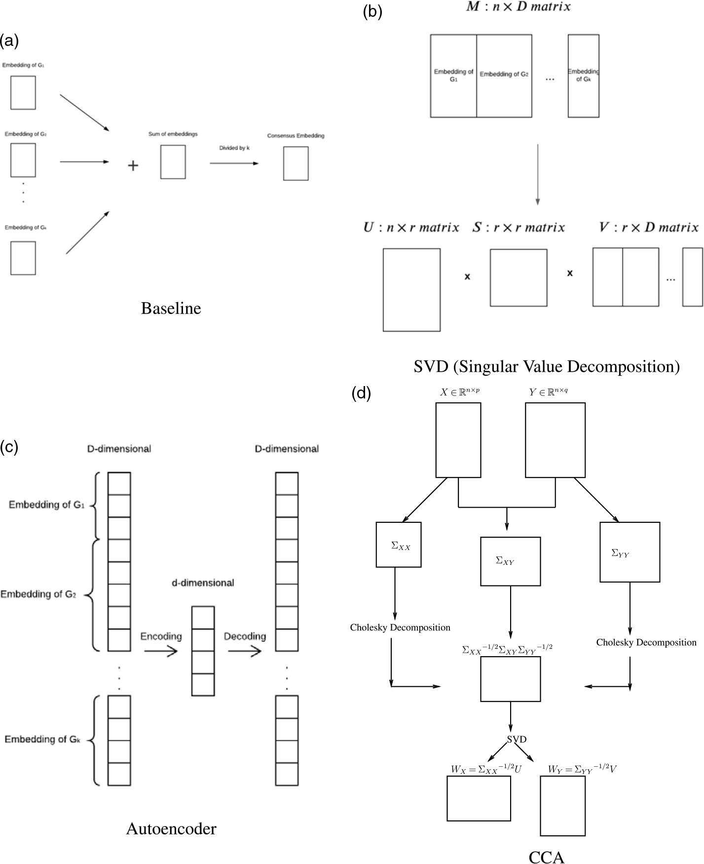
3.1.1 Baseline consensus embedding:
The baseline embedding we consider assumes that the embeddings of individual network versions represent similar spaces and the dimensions of the embeddings align with each other (Park et al., Reference Park, Kim, Han and Yu2020). This requires that $d_1=d_2=...=d_k=d$
. Thus, provided that the embeddings of invidiual versions have the same number of dimensions, we compute the baseline embedding as follows:
$d_1=d_2=...=d_k=d$
. Thus, provided that the embeddings of invidiual versions have the same number of dimensions, we compute the baseline embedding as follows:
 \begin{equation} X_C^{(Baseline)}=\frac{\sum_{i=1}^{k}{X_k}}{k}.\end{equation}
3.1.2 Singular value decomposition (SVD):
SVD is a matrix decomposition method for reducing a matrix to its constituent parts. The singular value decomposition of an $m \times p$
matrix M, whose rank is r, is a factorization of the form
$m \times p$
matrix M, whose rank is r, is a factorization of the form $USV^T$
, where U is an
$USV^T$
, where U is an $m \times r$
unitary matrix, S is an
$m \times r$
unitary matrix, S is an $r \times r$
diagonal matrix, and V is an
$r \times r$
diagonal matrix, and V is an $p \times r$
unitary matrix. S is a diagonal matrix and the diagonal values of S are called the singular values of M.
$p \times r$
unitary matrix. S is a diagonal matrix and the diagonal values of S are called the singular values of M.
Let X be the $n\times D$
matrix obtained by concatenating
$n\times D$
matrix obtained by concatenating $X_1$
,
$X_1$
, $X_2$
, …,
$X_2$
, …, $X_k$
, where
$X_k$
, where $D=d_1+d_2+...+d_k$
. If we set our objective as one of choosing an
$D=d_1+d_2+...+d_k$
. If we set our objective as one of choosing an $n\times D$
matrix Y with rank d to minimize the Frobenius or 2-norm of the difference
$n\times D$
matrix Y with rank d to minimize the Frobenius or 2-norm of the difference $||X-Y||$
, then the optimal solution is given by the truncation of the SVD of X to the largest d singular values (and corresponding singular vectors) of X.
$||X-Y||$
, then the optimal solution is given by the truncation of the SVD of X to the largest d singular values (and corresponding singular vectors) of X.
In other words, letting $M=X$
in the formulation of SVD, we obtain
$M=X$
in the formulation of SVD, we obtain $n\times r$
dimensional matrix U,
$n\times r$
dimensional matrix U, $r\times r$
dimensional matrix S, and
$r\times r$
dimensional matrix S, and $D\times r$
dimensional matrix V, where r denotes the rank of X and
$D\times r$
dimensional matrix V, where r denotes the rank of X and $X=USV^T$
. Now let U’, S’, and V’ denote the
$X=USV^T$
. Now let U’, S’, and V’ denote the $n\times d$
,
$n\times d$
, $d\times d$
, and
$d\times d$
, and $D \times d$
matrices obtained by choosing the first d columns (also rows for S) of, respectively, U, S, and V. Then the matrix
$D \times d$
matrices obtained by choosing the first d columns (also rows for S) of, respectively, U, S, and V. Then the matrix $Y=U'S'V'^T$
provides the best rank-d approximation to X. Consequently, V’ provides an optimal mapping of the D dimensions in X to d-dimensional space. Based on this observation, SVD-based dimensionality reduction sets
$Y=U'S'V'^T$
provides the best rank-d approximation to X. Consequently, V’ provides an optimal mapping of the D dimensions in X to d-dimensional space. Based on this observation, SVD-based dimensionality reduction sets
 \begin{equation}X_c^{(SVD)} = XV'^T,\end{equation}
i.e., it maps the D-dimensional concatenated embedding of each node of the graph into the d-dimensional space defined by the SVD of X.
3.1.3 Variational autoencoder:
An autoencoder is an unsupervised learning algorithm that applies backpropagation to obtain a lower-dimensional representation of data, setting the target values to be equal to the inputs. The autoencoder is a neural network with D inputs, each representing a column of the matrix X (i.e., a dimension in one of the k embeddings spaces). The encoder layer(s) map these D inputs to d latent features shown in the middle, which are subsequently transformed into the D output by the decoder layer(s). While training the network, each row of the matrix X (i.e., the embedding of each node) is used as an input and the respective output. The neural network is trained using this loss function:
 \begin{equation} L(X,Y)=\|X-Y\|_F^2,\end{equation}
where Y denotes the $n\times D$
matrix whose rows represent the outputs of the network corresponding to the inputs that represent the rows of X. Thus, the idea behind the variational autoenconder is to learn an encoding of the D input dimensions into the d latent features (shown in the middle) such that the D inputs can be reconstructed by the decoder with minimum loss. Observe that this loss function is identical to that of SVD; however, the use of neural networks provides the ability to perform nonlinear dimensionality reduction. Once the neural network is trained, we perform dimensionality reduction by retaining the d-dimensional output of the encoder that corresponds to each of the n training instances (rows of the matrix X or nodes in V). These n d-dimensional vectors comprise the matrix
$n\times D$
matrix whose rows represent the outputs of the network corresponding to the inputs that represent the rows of X. Thus, the idea behind the variational autoenconder is to learn an encoding of the D input dimensions into the d latent features (shown in the middle) such that the D inputs can be reconstructed by the decoder with minimum loss. Observe that this loss function is identical to that of SVD; however, the use of neural networks provides the ability to perform nonlinear dimensionality reduction. Once the neural network is trained, we perform dimensionality reduction by retaining the d-dimensional output of the encoder that corresponds to each of the n training instances (rows of the matrix X or nodes in V). These n d-dimensional vectors comprise the matrix $X_C^{(VAE)}$
, i.e, consensus embeddings of the nodes in V computed by variational autoencoder.
$X_C^{(VAE)}$
, i.e, consensus embeddings of the nodes in V computed by variational autoencoder.
In our implementation, we use a convolutional autoencoder (Masci et al., Reference Masci, Meier, Cire?an and Schmidhuber2011). Same as a standard autoencoder, a convolutional autoencoder also aims to output the same vectors as the input. The convolutional autoencoder contains convolutional layers in the encoder part of the autoencoder. In every convolutional layer, there is a filter that slides around the input matrix to compute the next layer. Convolutional autoencoder also have pooling layers after each convolutional layer. In the decoder part, there are deconvolutional layers and unpooling layers that recovers the input matrix.
3.1.4 Canonical correlation analysis (CCA):
Given two embedding matrices, $X_1 \in \mathbb{R}^{n\times d_1}$
and
$X_1 \in \mathbb{R}^{n\times d_1}$
and $X_2 \in \mathbb{R}^{n\times d_2}$
, computed by any embedding algorithm, such as node2vec (Grover & Leskovec, Reference Grover and Leskovec2016) for
$X_2 \in \mathbb{R}^{n\times d_2}$
, computed by any embedding algorithm, such as node2vec (Grover & Leskovec, Reference Grover and Leskovec2016) for $G_1 = (V, E_1)$
and
$G_1 = (V, E_1)$
and $G_2 = (V, E_2)$
, respectively. Our objective is to compute an
$G_2 = (V, E_2)$
, respectively. Our objective is to compute an $n\times d$
embedding matrix, where
$n\times d$
embedding matrix, where $d=\min\{d_1,d_2\}$
, such that intrinsic information encoded in each of these embedding matrices is preserved.
$d=\min\{d_1,d_2\}$
, such that intrinsic information encoded in each of these embedding matrices is preserved.
CCA aims to find low-dimensional latent representations, $W_1 \in \mathbb{R}^{d_1 \times d}$
and
$W_1 \in \mathbb{R}^{d_1 \times d}$
and $W_2 \in \mathbb{R}^{d_2 \times d}$
, such that cosine angles between
$W_2 \in \mathbb{R}^{d_2 \times d}$
, such that cosine angles between ${W_1}^T X_1(i)$
and
${W_1}^T X_1(i)$
and ${W_2}^T X_2(i)$
is minimized, where
${W_2}^T X_2(i)$
is minimized, where $X_1(i)$
and
$X_1(i)$
and $X_2(i)$
denote the vectors containing the ith rows of the respective matrices (Uurtio et al., Reference Uurtio, Monteiro, Kandola, Shawe-Taylor, Fernandez-Reyes and Rousu2017), i.e. they are the embeddings of the same node in two different versions of the network.
$X_2(i)$
denote the vectors containing the ith rows of the respective matrices (Uurtio et al., Reference Uurtio, Monteiro, Kandola, Shawe-Taylor, Fernandez-Reyes and Rousu2017), i.e. they are the embeddings of the same node in two different versions of the network.
We first discuss the case for $d=1$
for ease of exposition, and then generalize to the case
$d=1$
for ease of exposition, and then generalize to the case $d\geq 2$
. Minimizing the cosine of the angle between two vectors can also be thought as minimizing Euclidean distance between the vectors in a unit-ball. Thus, we can state CCA’s objective as follows:
$d\geq 2$
. Minimizing the cosine of the angle between two vectors can also be thought as minimizing Euclidean distance between the vectors in a unit-ball. Thus, we can state CCA’s objective as follows:
 \begin{equation}\begin{aligned}({W_1}^*, {W_2}^*): =& \underset{W_1, W_2}{\text{argmin}}& & \dfrac{1}{n} \sum_{i = 1}^n {({W_1}^T X_1(i) - {W_2}^T X_2(i))}^2 \\& \text{subject to}& & {\left\lVert {W_1}^T X_1(i)\right\rVert}_2 = 1 ,{\left\lVert W_2 X_2(i)\right\rVert}_2 = 1.\end{aligned}\end{equation}
By using the sample covariance matrix definition and ignoring constant terms, we can restate CCA’s objective function as a maximization problem (Uurtio et al., Reference Uurtio, Monteiro, Kandola, Shawe-Taylor, Fernandez-Reyes and Rousu2017). Furthermore, we can extend the optimization problem to the case with $d\geq 2$
, by adding the additional constraint that the columns of
$d\geq 2$
, by adding the additional constraint that the columns of $W_1$
and
$W_1$
and $W_2$
are orthogonal:
$W_2$
are orthogonal:
 \begin{equation}\begin{aligned}({W_1}^*, {W_2}^*): =& \underset{W_1, W_2}{\text{argmax}}& & {W_1}^T {\Sigma}_{12} {W_2} \\& \text{subject to}& & {W_1}^T {\Sigma}_{11} {W_1} = I, {W_2}^T {\Sigma}_{22} {W_2} = I.\end{aligned}\end{equation}
where ${\Sigma}_{11} = \dfrac{1}{n} \sum_{i = 1}^n X_1 {X_1}^T$
,
${\Sigma}_{11} = \dfrac{1}{n} \sum_{i = 1}^n X_1 {X_1}^T$
, ${\Sigma}_{22} = \dfrac{1}{n} \sum_{i = 1}^n X_2(i) {X_2(i)}^T$
and
${\Sigma}_{22} = \dfrac{1}{n} \sum_{i = 1}^n X_2(i) {X_2(i)}^T$
and ${\Sigma}_{12} = \dfrac{1}{n} \sum_{i = 1}^n X_1(i) {X_2(i)}^T$
are sample covariance matrices. By using Lagrange duality, this problem can be solved as a generalized eigenvalue problem or SVD (Uurtio et al., Reference Uurtio, Monteiro, Kandola, Shawe-Taylor, Fernandez-Reyes and Rousu2017).
${\Sigma}_{12} = \dfrac{1}{n} \sum_{i = 1}^n X_1(i) {X_2(i)}^T$
are sample covariance matrices. By using Lagrange duality, this problem can be solved as a generalized eigenvalue problem or SVD (Uurtio et al., Reference Uurtio, Monteiro, Kandola, Shawe-Taylor, Fernandez-Reyes and Rousu2017).
Namely, letting $B={\Sigma_{11}}^{-1/2} \Sigma_{12} {\Sigma_{22}}^{-1/2}$
and computing the SVD of matrix B as
$B={\Sigma_{11}}^{-1/2} \Sigma_{12} {\Sigma_{22}}^{-1/2}$
and computing the SVD of matrix B as $B=U_B^{T} S_B V_B$
, the best projection matrices sought by CCA are given as:
$B=U_B^{T} S_B V_B$
, the best projection matrices sought by CCA are given as:
 \begin{equation}W_1 = {\Sigma_{11}}^{-1/2} U_B, W_2 = {\Sigma_{22}}^{-1/2} V_B.\end{equation}
Finally, after computing $W_1$
and
$W_1$
and $W_2$
using the above framework, we construct consensus embedding of
$W_2$
using the above framework, we construct consensus embedding of $G_1$
and
$G_1$
and $G_2$
as
$G_2$
as
 \begin{equation} X_c^{(CCA)} = ({W_1}^T X_1 + {W_2}^T Y_2) / 2.\end{equation}
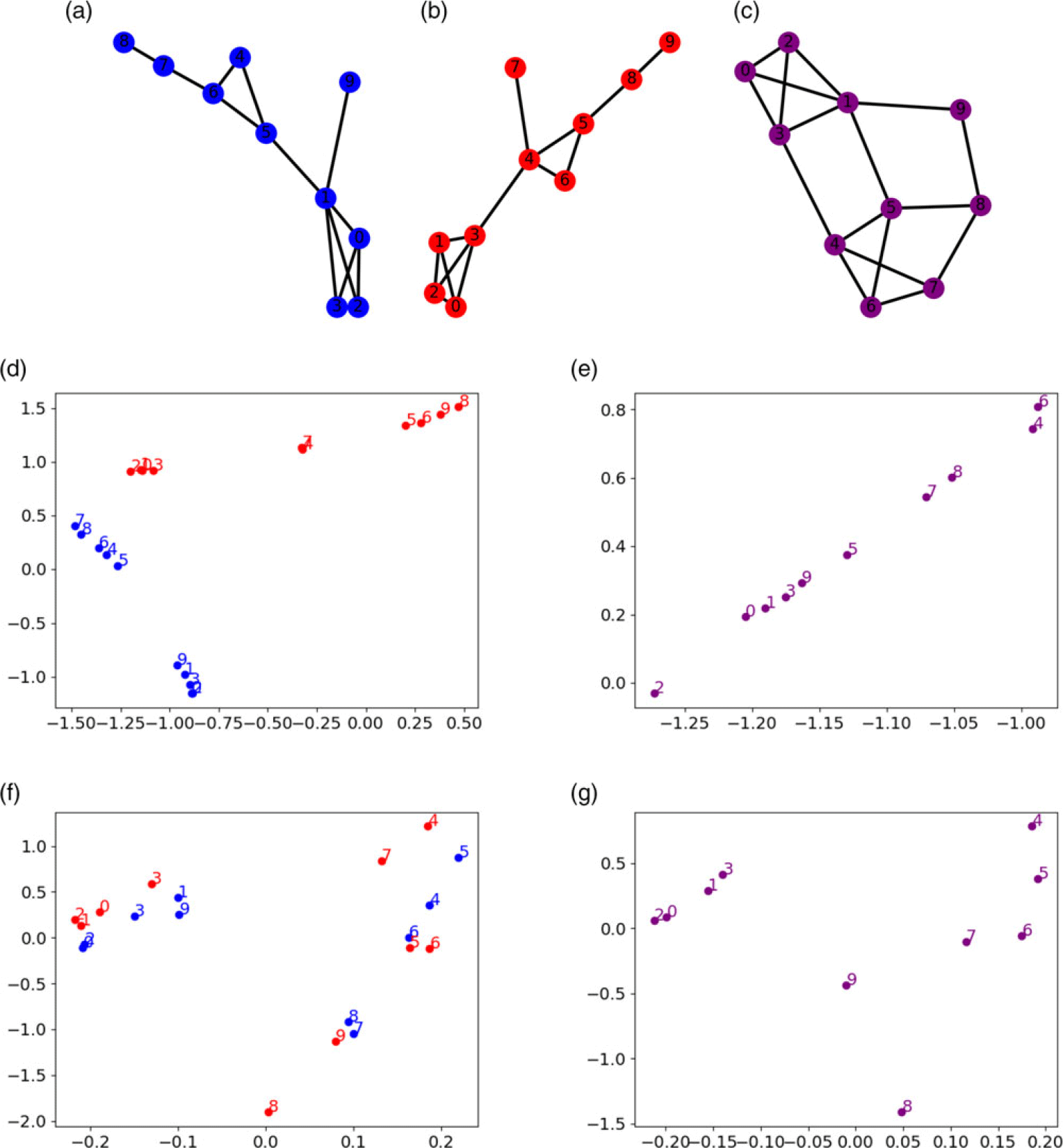
An illustration of the application of CCA to the computation of consensus embeddings is illustrated in Figure 3. The two versions of the network, $G_1$
and
$G_1$
and $G_2$
are shown in Figure 3(a) and (b), respectively. The integrated network obtained by superposing these two versions is shown in Figure 3(c). The two-dimensional embeddings of the two versions are shown in Figure 3(c). Clearly, these embeddings are in different spaces, so we arbitrarily match the dimensions of the two embeddings. The
$G_2$
are shown in Figure 3(a) and (b), respectively. The integrated network obtained by superposing these two versions is shown in Figure 3(c). The two-dimensional embeddings of the two versions are shown in Figure 3(c). Clearly, these embeddings are in different spaces, so we arbitrarily match the dimensions of the two embeddings. The $10\times 2$
matrices
$10\times 2$
matrices ${W_1}^T X_1$
and
${W_1}^T X_1$
and ${W_2}^T Y_2$
are visualized in Figure 3(f). This represents the projection of the embeddings of the two versions to the common space computed by CCA. As seen in the figure, the points that correspond to the same node are brought close together, as captured by the objective function of CCA. The consensus embedding,
${W_2}^T Y_2$
are visualized in Figure 3(f). This represents the projection of the embeddings of the two versions to the common space computed by CCA. As seen in the figure, the points that correspond to the same node are brought close together, as captured by the objective function of CCA. The consensus embedding, $X_c^{(CCA)}$
, is computed by taking the mean of the two points that correspond to each node, and is shown in Figure 3(g). The two-dimensional embedding of the integrated network is shown in Figure 3(c). Comparison of the two embeddings shows that CCA is able to reconstruct the overall structure of the embeddings, with the nodes in the two communities mapped close to each other.
$X_c^{(CCA)}$
, is computed by taking the mean of the two points that correspond to each node, and is shown in Figure 3(g). The two-dimensional embedding of the integrated network is shown in Figure 3(c). Comparison of the two embeddings shows that CCA is able to reconstruct the overall structure of the embeddings, with the nodes in the two communities mapped close to each other.
The computation of consensus embeddings using Canonical Correlation Analysis (CCA). (a, b) Red and blue networks with identical sets of nodes labeled from 1 to 10. (c) The integrated network obtained by superposing the two networks. (d) 2D embeddings of the individual networks. Note that the embeddings are in different spaces and we arbitrarily match dimensions of embeddings to plot them in the same space. The colors and the numbers show the identity of the nodes and the network each node belongs to. (e) 2D embedding of the integrated network. (f) The embeddings of the two networks after space transformation via CCA. (g) The consensus embedding computed by taking the mean of the two transformed embeddings.
The effect of CCA on multidimensional embeddings is illustrated in Figure 4(a). Given two matrices (here we use two embeddings), the correlations between the dimensions do not have any patterns (left panel in Figure 4(a)), i.e., the dimensions of the embeddings do not have a clear correspondence. After application of CCA, the correlations between the corresponding dimensions (diagonal of the matrix) become larger, and the correlations of the pairs other than corresponding dimensions are all close to 0.
The correspondence between the dimensions of embeddings computed on two or multiple different networks. (a) The correlation matrix of the 16 embedding dimensions for the embeddings computed on $G_1$
and
$G_1$
and $G_2$
(Table 1). (b) The correlation matrix of the 16 embedding dimensions after transformation via cannonical correlation analysis (CCA). (c) The pairwise correlation matrices of the 16 embedding dimensions for the embeddings
$G_2$
(Table 1). (b) The correlation matrix of the 16 embedding dimensions after transformation via cannonical correlation analysis (CCA). (c) The pairwise correlation matrices of the 16 embedding dimensions for the embeddings $G_1$
,
$G_1$
, $G_2$
, and
$G_2$
, and $G_3$
before (top) and after (bottom) transformation via Generalized Canonical Correlation Analysis (GCCA).
$G_3$
before (top) and after (bottom) transformation via Generalized Canonical Correlation Analysis (GCCA).

3.1.5 Generalized canonical correlation analysis (GCCA):
Since CCA is designed to work with two vector spaces, it can be applied to the computation of consensus embeddings with two network versions. To compute consensus embeddings for $k > 2$
dimensions, the framework needs to be generalized.
$k > 2$
dimensions, the framework needs to be generalized.
Generalized CCA (Kettenring et al., 1971) is a method that applies CCA on more than two matrices. Let $G_1, G_2, ..., G_k$
denote the k versions of a network with n nodes. Assume that we have the k respective embeddings
$G_1, G_2, ..., G_k$
denote the k versions of a network with n nodes. Assume that we have the k respective embeddings $X_1, X_2, ... , X_k$
available, where the embeddings are, respectively,
$X_1, X_2, ... , X_k$
available, where the embeddings are, respectively, $d_1, d_2, ... , d_k$
dimensional. GCCA learns the following optimization problem:
$d_1, d_2, ... , d_k$
dimensional. GCCA learns the following optimization problem:
 \begin{equation} \min_{Z_i,A}\sum_{i=1}^k \|A - Z_i^TX_i\|^2\end{equation}
where $A \in \mathbb{R}^{d \times n}$
is a shared representation of the n embedding spaces, and
$A \in \mathbb{R}^{d \times n}$
is a shared representation of the n embedding spaces, and $Z_i \in \mathbb{R}^{d_i \times d}$
are the individual projection matrices for each embedding. Once A and
$Z_i \in \mathbb{R}^{d_i \times d}$
are the individual projection matrices for each embedding. Once A and $Z_i$
’s are computed, we use the mean of the projected embeddings as the consensus embedding, i.e.
$Z_i$
’s are computed, we use the mean of the projected embeddings as the consensus embedding, i.e.
 \begin{equation}X_c = (Z_1^TX_1+ Z_2^TX_2+ \cdots + Z_k^TX_k)/k.\end{equation}
Figure 4(b) illustrates the effect of GCCA on the correlations between dimensions. Given three 16-dimensional embeddings $X_1, X_2, X_3$
, the correlations between
$X_1, X_2, X_3$
, the correlations between $\{X_1,X_2\}$
,
$\{X_1,X_2\}$
, $\{X_1,X_3\}$
, and
$\{X_1,X_3\}$
, and $\{X_2,X_3\}$
are shown in the upper panel of Figure 4(b). We can see no patterns in the three matrices. However, after using GCCA, we get the lower panel of Figure 4(b). The darkest parts of those three matrices appear close to their diagonals.
$\{X_2,X_3\}$
are shown in the upper panel of Figure 4(b). We can see no patterns in the three matrices. However, after using GCCA, we get the lower panel of Figure 4(b). The darkest parts of those three matrices appear close to their diagonals.
We use the software (Jameschapman19, 2020) in our implementations of CCA and GCCA consensus embedding. It provides the implementations of multiple kinds of CCA-related methods.
3.2 Processing combinatorial link prediction queries for versioned networks
Consider the following scenario: A graph database houses k versions of a network (as formulated at the beginning of this section). These k versions may either come from different resources (e.g., different protein–protein interaction databases) or represent semantically different types of edges between a common set of nodes (e.g., genetic interactions vs. physical interactions vs. functional association among human proteins). In this setting, a “combinatorial” link prediction query can be formulated as follows: The user chooses (i) a node $q \in V$
, and (ii) a subset
$q \in V$
, and (ii) a subset $S \subseteq \{G_1, G_2, ..., G_k\}$
of networks. The query seeks to identify the nodes that are most likely to be associated with the query node q based on the topology of the integrated network
$S \subseteq \{G_1, G_2, ..., G_k\}$
of networks. The query seeks to identify the nodes that are most likely to be associated with the query node q based on the topology of the integrated network $G^{(S)}=(V, E^{(S)})$
, where
$G^{(S)}=(V, E^{(S)})$
, where $E^{(S)}=\bigcup_{i\in S}{E_i}$
. Such a flexible query framework is highly useful in the context of many applications, since the relevance and reliability of different network versions can be variable, and different users may have different needs and preferences.
$E^{(S)}=\bigcup_{i\in S}{E_i}$
. Such a flexible query framework is highly useful in the context of many applications, since the relevance and reliability of different network versions can be variable, and different users may have different needs and preferences.
The above framework defines a “combinatorial” query in the sense that a user can select any combination of networks to integrate. This poses a significant computational challenge as the number of possible combinations of networks is exponential in the number of networks in the database, i.e., the user can choose from $2^k-1$
possible combinations of networks.
$2^k-1$
possible combinations of networks.
Embedding-based link prediction can facilitate the development of effective solutions to the combinatorial challenge associated with combinatorial link prediction queries, because link prediction algorithms using node embeddings do not need to access to the network topology while performing link prediction. By computing and storing node embeddings in advance, it is possible to efficiently process link prediction queries while giving the user the flexibility to choose the combination of networks to integrate.
Consensus embeddings provide an alternate solution that can render storage feasible while enabling real-time query processing for very large networks and large number of versions: Compute and store the embeddings for each network separately. When the user selects a combination, compute a consensus embedding for that combination and use it to process the query. One important consideration in the application of this idea is the “inexact” nature of consensus embeddings, i.e., consensus embeddings may not adequately capture the information represented by the embeddings computed on the integrated network.
4 Experimental results
In our experiments, we try to predict new links in the integrated network of multiple networks. We use BioNEV to split multiple input graphs into training and testing sets, and compute the consensus embedding of the training graphs. Then the consensus embedding of the training graphs are used as an input of BioNEV evaluation to predict all the testing edges from the multiple graphs.
4.1 Datasets
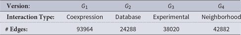
In our computational experiments, we use human protein–protein interaction (PPI) networks obtained from BioGRID (Stark et al., Reference Stark, Breitkreutz, Reguly, Boucher, Breitkreutz and Tyers2006) and yeast PPI networks from STRING (Franceschini et al., Reference Franceschini, Szklarczyk, Frankild, Kuhn, Simonovic and Roth2012; Cho et al., Reference Cho, Berger and Peng2016). PPI networks contain physical interactions and functional associations between pairs of proteins. The human PPI dataset we use contains multiple PPI networks separated based on experimental systems. Each network (version) contains a unique type of PPI (genetic or physical). The yeast PPI network dataset contains four PPI networks derived from different sources (e.g. experimental data, or curated database). The types of the interactions represented by each network version are shown in Tables 1 and 2. In order to obtain multiple networks with the same set of nodes, we remove the nodes (proteins) that do not exist in all versions. After preprocessing, all the human PPI versions have 1025 nodes, and all the yeast PPI versions have 1164 nodes. The type of PPI and the number of edges for each network are shown in Tables 1 and 2.
The description and size of the human protein–protein interaction (PPI) networks used in our experiments

The description and size of the yeast protein–protein interaction (PPI) networks used in our experiments
4.2 Experimental setup
We compare the link prediction performance of the node embeddings computed on integrated networks and consensus embeddings computed based on the embeddings of individual networks. We consider two embedding algorithms, Node2vec (Grover & Leskovec, Reference Grover and Leskovec2016) and Role2vec (Ahmed et al., Reference Ahmed, Rossi, Lee, Willke, Zhou, Kong and Eldardiry2019), and multiple methods for computing consensus embeddings, SVD, variational autoencoder, CCA (or GCCA for more than two versions), and baseline(average).
To assess link prediction performance, we use BioNEV(Yue et al., Reference Yue, Wang, Huang, Parthasarathy, Moosavinasab and Huang2020), a Python package that is developed to assess the performance of various tasks that utilize network embeddings. The software splits an input graph into a training graph and a testing edge set. BioNEV uses the known interactions as positive samples and randomly selects the negative samples. Both samples are split into a training set (80%) and a testing set (20%). For each node pair, BioNEV concatenates the embeddings of two nodes as the edge feature and then build a binary classifier. It outputs the AUCs of the link predictions using the embeddings.
In the experiments focusing on the consensus embeddings of pairs of versions, we are given two embeddings $X_1 \in \mathbb{R}^{n \times d_1}$
and
$X_1 \in \mathbb{R}^{n \times d_1}$
and $X_2 \in \mathbb{R}^{n \times d_2}$
, we compute the consensus embedding
$X_2 \in \mathbb{R}^{n \times d_2}$
, we compute the consensus embedding $X_c \in \mathbb{R}^{n \times d}$
, in which
$X_c \in \mathbb{R}^{n \times d}$
, in which $d = \min\{d_1,d_2\}$
. We show results for cases
$d = \min\{d_1,d_2\}$
. We show results for cases $d1=d2$
or
$d1=d2$
or $d1\neq d2$
, and compare different dimensionality reduction methods. Note that, when
$d1\neq d2$
, and compare different dimensionality reduction methods. Note that, when $d1\neq d2$
, the baseline method for computing consensus embeddings does not apply as it requires the embeddings to have equal number of dimensions.
$d1\neq d2$
, the baseline method for computing consensus embeddings does not apply as it requires the embeddings to have equal number of dimensions.
For multiple (more than two) networks, we consider the case where all embeddings have the same number of dimensions, and the number dimensions of the consensus embedding is the same as the embeddings of individual versions.
4.3 Link prediction for pairs of versions
As mentioned before, the dimensions of the individual embeddings can be the same or different. In this section, we show the results of pairs of versions for both same numbers of dimensions and different numbers of dimensions. We compute the consensus embedding of all combinations of two networks from Table 1 (eight versions with 28 pairs), and get their link prediction accuracies by BioNEV.
4.3.1 Two embeddings with same dimensions
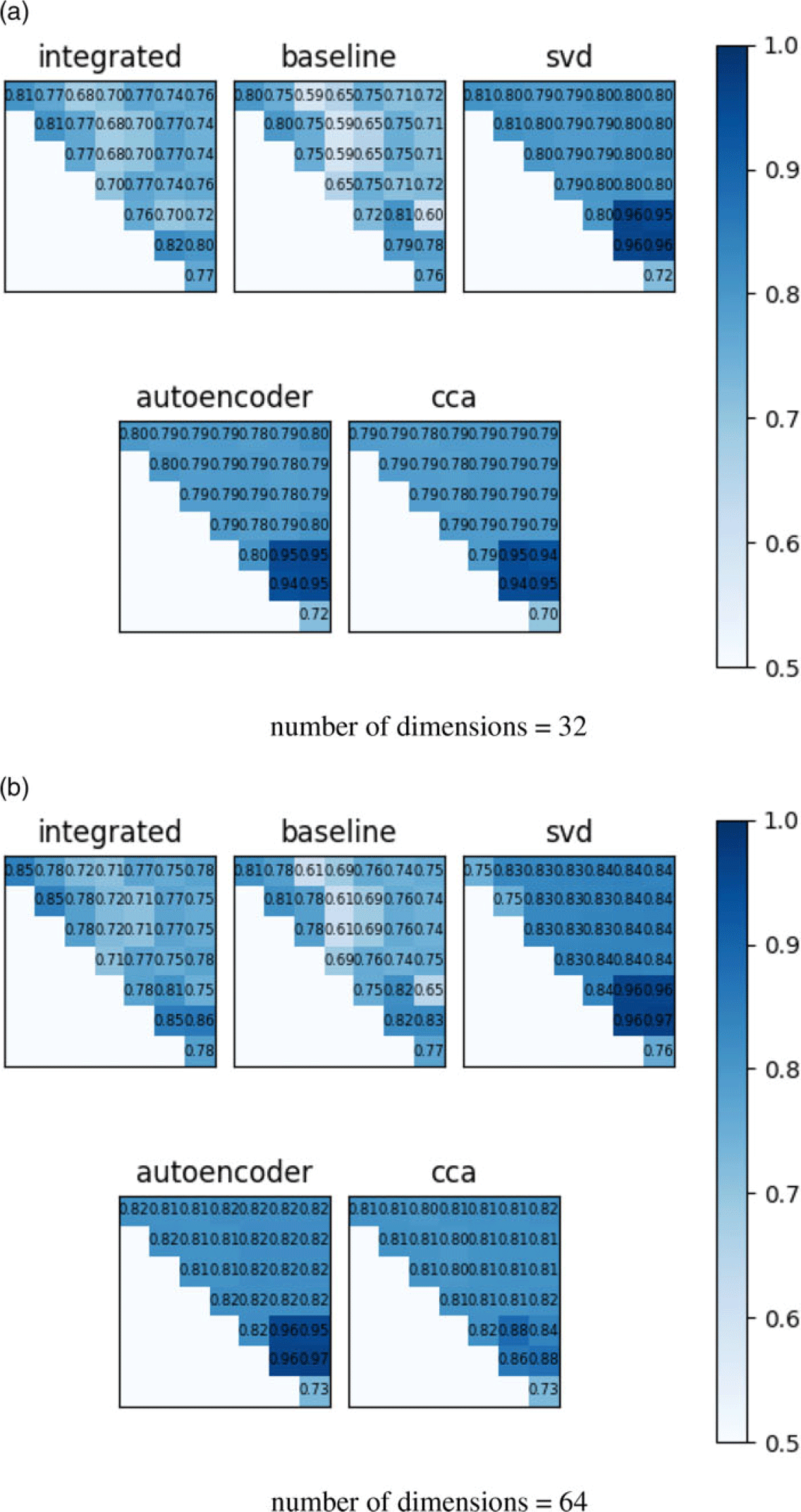
We test all the combinations of the eight versions described in Table 1. Figure 5 shows the AUCs provided by the consensus embeddings computed using four different methods, compared with the AUC of the embedding of the integrated network. The embedding algorithm used in the figure is node2vec. For most network pairs, consensus embeddings deliver better link prediction accuracy than the integrated network’s own embeddings. Among the three dimensionality reduction methods, SVD and CCA are more stable and consistently deliver better accuracy than variational autoencoder. As expected, the accuracy of the baseline consensus embedding (the average of the pair of embeddings) is much lower, but is still better than would be expected at random. This suggests that there can be some correspondence between the embedding spaces of different network versions.
Link prediction accuracy of consensus embeddings on pairs of networks with equal number of dimensions for individual node embeddings. All embeddings are computed using node2vec and results are displayed for (a) 32-dimensional and (b) 64-dimensional embeddings. Each matrix shows the link prediction accuracy, assessed in terms of area under ROC curve (AUC), of the respective embeddings for all $\binom{8}{2}=28$
pairs of networks. Integrated: The embedding of the network obtained by superposing the two networks. Baseline: The consensus embedding obtained by averaging the embeddings of the two networks. SVD, Autoencoder, CCA: The consensus embedding computed using each of the three dimensionality reduction methods we consider. Darker shade of blue indicates more accurate prediction performance.
$\binom{8}{2}=28$
pairs of networks. Integrated: The embedding of the network obtained by superposing the two networks. Baseline: The consensus embedding obtained by averaging the embeddings of the two networks. SVD, Autoencoder, CCA: The consensus embedding computed using each of the three dimensionality reduction methods we consider. Darker shade of blue indicates more accurate prediction performance.
4.3.2 Two embeddings with different dimensions
Figure 6 shows the link prediction results of consensus embeddings for pairs of networks when the numbers of dimensions of two embeddings are not the same. From Figure 6, the average accuracy of consensus embedding using CCA is higher than SVD or autoencoder. The data points of SVD or autoencoder are sparser in the range, and the lowest point is between 0.55 and 0.6. Unlike SVD or autoencoder, all data points of CCA are above 0.65, and most of them are in the range of (0.70, 0.75).
Link prediction accuracy of consensus embeddings of pairs on networks with different number of dimensions in individual embeddings. Each beeswarm plots shows the distribution of area under ROC curve (AUC) for the link prediction performance of consensus embeddings computed using SVD (blue), Autoencoder (orange), CCA (green) across $8\times7=56$
(ordered) pairs of networks. Each panel shows a different number of dimensions for the individual embeddings of each network: (a) 16 vs. 32, (b) 16 vs. 64, (c) 16 vs. 128, (d) 32 vs. 64, (e) 32 vs. 128, (f) 64 vs. 128.
$8\times7=56$
(ordered) pairs of networks. Each panel shows a different number of dimensions for the individual embeddings of each network: (a) 16 vs. 32, (b) 16 vs. 64, (c) 16 vs. 128, (d) 32 vs. 64, (e) 32 vs. 128, (f) 64 vs. 128.

4.4 Link prediction for multiple versions
Our experiments for multiple ( $> 2$
) networks are based on all combinations of the datasets (8 versions with 247 potential combinations).
$> 2$
) networks are based on all combinations of the datasets (8 versions with 247 potential combinations).
Figure 7 shows the link prediction results of consensus embeddings of more than two versions. In these experiments, we use GCCA instead of CCA even for two versions. In each figure, the AUC of link prediction is shown as a function of the number of network versions. We observe that, on average, the accuracy of link prediction goes down with increasing number of versions that are integrated. However, the performance difference between embedding of integrated network and consensus embeddings are not very large. This observation suggests that the utility of concensus embeddings can be more pronounced for network databases with larger number of versions.
Accuracy of consensus embeddings in link prediction as a function of the number of networks that are integrated. The dataset of the experiments are the human PPI networks. Results are shown for Node2vec and Role2vec. For each point k on the x axis, each point in the plot shows the area under ROC curve (AUC) of link prediction for a specific combination of k network versions for $1\leq k \leq 8$
. The lines show the average AUC across all combinations. The blue, yellow, red, and green points/lines, respectively, show the accuracy provided by the embeddings computed directly on the integrated network, consensus embeddings computed using SVD, consensus embeddings computed using variational autoencoder, consensus embeddings computed using GCCA, and the baseline consensus embedding (average of individual embeddings).
$1\leq k \leq 8$
. The lines show the average AUC across all combinations. The blue, yellow, red, and green points/lines, respectively, show the accuracy provided by the embeddings computed directly on the integrated network, consensus embeddings computed using SVD, consensus embeddings computed using variational autoencoder, consensus embeddings computed using GCCA, and the baseline consensus embedding (average of individual embeddings).

As seen in Figure 7, accuracy of link prediction is improved with increasing number of dimensions in node embeddings. The embedding of the integrated network is the most accurate one in most cases. The link prediction accuracy of GCCA is better in lower cases, and it exceeds the accuracy of the integrated network when number of dimensions is 16. In larger numbers of dimensions, SVD and autoencoder perform better than GCCA.
In this part, we include another embedding method, role2vec, to show that consensus embedding also works for other embedding methods. GCCA performs better than SVD or variational autoencoder when used in consensus embedding of role2vec. Also, in the results of role2vec, the accuracy of consensus embedding become closer and closer to the accuracy of the embedding of the integrated network as the number of dimensions goes higher.
We also plot the AUC as a function of dimensions (Figures 8 and 9). We take all the networks in each dataset and compute the consensus embeddings by different methods. In general, the AUC increases as the number of dimensions increases for both node2vec and role2vec. When the number of dimensions reaches 128, the accuracy does not increase as much as the lower dimensions, so we might not gain much accuracy improvement when we use too large dimensions. In Figure 8, the performance of the integrated networks’ embeddings is better than consensus embeddings, but GCCA outperforms the integrated network in Figure 9, especially for role2vec.
The link prediction accuracies as a function of dimensions for the human PPI data (table 1). Results are shown for Node2vec and Role2vec. The plot shows the link prediction AUC of the consensus embeddings of all the versions when the numbers of dimensions are 16, 32, 64, and 128.

The link prediction accuracies as a function of dimensions for the yeast PPI dataset (table 2). Results are shown for Node2vec and Role2vec. The plot shows the link prediction AUC of the consensus embeddings of all the versions when the numbers of dimensions are 16, 32, 64, and 128.
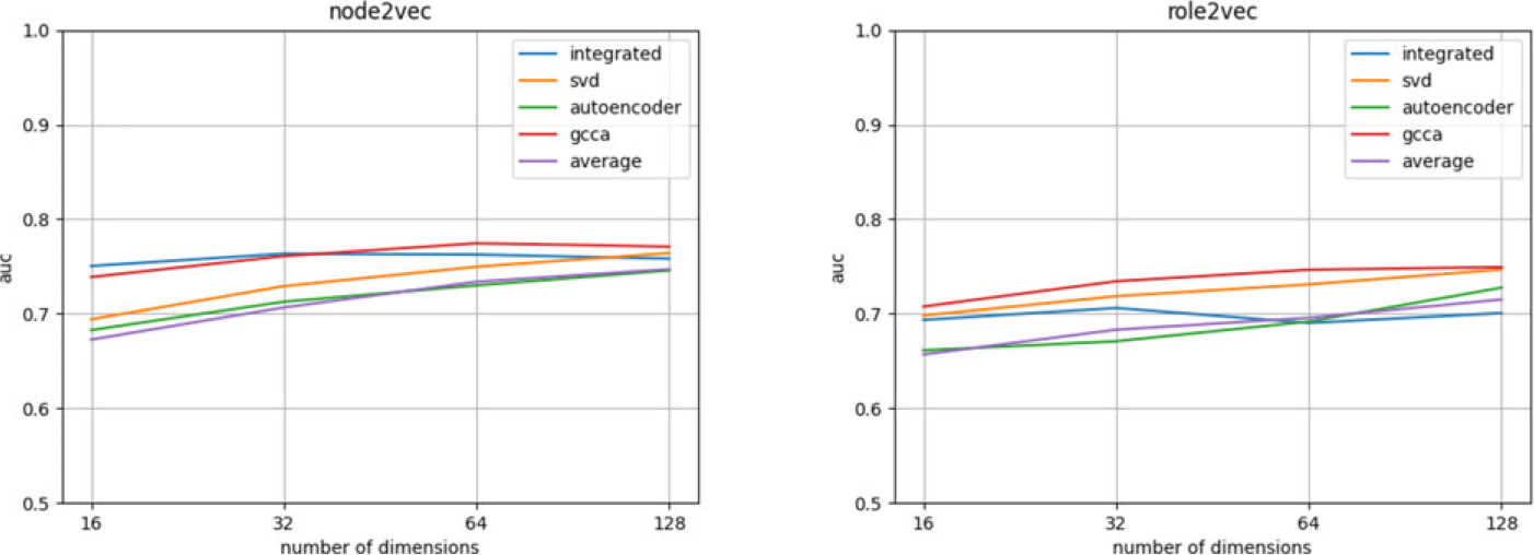
From these results, consensus embedding performs good or even better than the embedding of the integrated networks. Among the three kinds of dimensionality reduction methods, the results of SVD and variational autoencoder are similar in most experiments, and GCCA is the best one in most cases. Average might work well when the number of dimensions is low, but becomes worse when the number of dimensions is higher. For role2vec, average is always the worst among all the methods.
4.5 Runtime analysis
In this section, we investigate whether consensus embeddings improve the efficiency of processing link prediction queries. For this purpose, we compare the query processing time for consensus embeddings computed using different methods (SVD, autoencoder, and so on) against embeddings computed at query time after integrating the combination of networks selected by the user.
The results of this analysis are shown in Figure 10. As seen in the figure, processing queries using consensus embeddings drastically improves the efficiency of query processing. “Consensus Embedding at Query Time” using SVD enables processing of combinatorial link prediction queries in real time across the board, while integration of networks at query time requires orders of magnitude more time to process these queries. In most cases, “Consensus Embedding at Query Time” of convolutional autoencoder is also faster than “Network Integration at Query Time”, but its performance degrades with increasing number of networks that are being integrated. Also, the runtime becomes longer when the number of dimensions goes higher.
Runtime of combinatorial link prediction queries using consensus embeddings. The blue dots (for each combination)/curves (average of all combinations with the respective number of versions) show the query time corresponding to the “Network Integration at Query Time” approach described in Section 3.2, while the red and yellow dots/curves show the query time corresponding to the “Consensus Embedding at Query Time”. Results are shown for Node2vec and Role2vec, using four methods for computing consensus embeddings: SVD (yellow), Autoencoder (red), GCCA (green), and baseline concensus embedding (orange). The number of dimensions of the plots are 64.

The runtime of computing an embedding increases as networks become denser, especially for node2vec, because node2vec runs random walks starting from every nodes. As seen in 10, the blue dots in the plots of node2vec are separated into two groups. This is because $G_4$
is extremely dense (see Table 1), making the integrated networks that contain
$G_4$
is extremely dense (see Table 1), making the integrated networks that contain $G_4$
also dense. Therefore, combinations that contain
$G_4$
also dense. Therefore, combinations that contain $G_4$
have a significantly higher query runtime as compared to those that do not contain
$G_4$
have a significantly higher query runtime as compared to those that do not contain $G_4$
. Computation of consensus embeddings using SVD or CCA/GCCA is more robust to this effect. Average of individual embeddings is the fastest, even much faster than SVD or CCA, and it is also very stable.
$G_4$
. Computation of consensus embeddings using SVD or CCA/GCCA is more robust to this effect. Average of individual embeddings is the fastest, even much faster than SVD or CCA, and it is also very stable.
5 Conclusions
In this work, we consider the problem of computing node embeddings for integrated networks derived from the multiple network versions. We focus on the performance of link prediction using consensus embeddings compared with using the embeddings of the integrated networks.
We introduce a new dimensionlity reduction method, CCA and GCCA, into the consensus embedding process, and generalized the method such that the input embeddings can have different dimensions. CCA performs better than SVD or autoencoder when the numbers of dimensions of the pairs of embeddings are different.
We test the performance of link prediction of the consensus embeddings and found that accuracy of consensus embeddings is similar with the accuracy of embeddings computed directly from the integrated network. When there are only two versions, consensus embedding (for embeddings of the same number of dimensions) performs better than the embedding of the integrated network in link prediction in almost all experimental tests. For more than two versions, consensus embeddings also perform good or even better than the embeddings of the integrated networks, and CCA/GCCA performs better than SVD or variational autoencoder in most cases, especially when the embedding method is role2vec.
From our results, linear methods like CCA/GCCA and SVD work better than nonlinear methods like autoencoder. We guess that there are two main reasons:
-
Network embedding algorithms use linear models to represent the proximity of nodes in a network, thus linear methods may perform better in computing consensus embeddings.
-
Autoencoder is a neural-network based method, thus it may need more training data, i.e. the networks we are working with may be too small (in terms of the number of nodes) or too sparse for them to learn reliable latent patterns. To this end, autoencoders require more hyperparameters to be tuned, e.g. the number of layers, and the dimensions of each layer, which may also have an adverse effect on their reliability.
Also, dimensionality reduction methods work better than using the average of the individuals in predicting new links. In general, consensus embedding performs good link prediction compared to the embeddings of the integrated networks, especially for smaller numbers of versions and larger numbers of dimensions.
Moreover, from our runtime analyses, consensus embedding is much more efficient than computing the embeddings of the integrated networks, especially for large networks.
Competing interests
None.


 Open access