


1. Introduction
We study the use of Granger causality (Granger, Reference Granger1969, Reference Granger1980; Caines, Reference Caines1976) as a means of uncovering an underlying causal structure in multivariate time series. There are two basic ideas behind Granger’s notion of causality. First, that causes should precede their effects. Second, that the cause of an event must be external to the event itself. Granger’s methodology uses these ideas to test a necessary condition of causation: whether forecasting a process $x_c$
(the purported caused process) using another process
$x_c$
(the purported caused process) using another process $x_e$
(the external, or purported causing process), in addition to its own history, is more accurate than using the past data of
$x_e$
(the external, or purported causing process), in addition to its own history, is more accurate than using the past data of $x_c$
alone. If
$x_c$
alone. If $x_e$
is in fact a cause of
$x_e$
is in fact a cause of $x_c$
then it must be that the combined estimator is more accurate. If our data of interest can be appropriately modeled as a multivariate process in which Granger’s test for causation is also sufficient, then Granger causality tests provide a means of defining a network of causal connections. The nodes of this network are individual stochastic processes, and the directed edges between nodes indicate Granger causal connections. This causality graph is the principal object of our study.
$x_c$
then it must be that the combined estimator is more accurate. If our data of interest can be appropriately modeled as a multivariate process in which Granger’s test for causation is also sufficient, then Granger causality tests provide a means of defining a network of causal connections. The nodes of this network are individual stochastic processes, and the directed edges between nodes indicate Granger causal connections. This causality graph is the principal object of our study.
In practice, the underlying causality graph cannot be observed directly, and its presence is inferred as a latent structure among observed time series data. This notion has been used in a variety of applications, for example, in Neuroscience as a means of recovering interactions amongst brain regions (Bressler & Seth, Reference Bressler and Seth2011; Korzeniewska et al., Reference Korzeniewska, Crainiceanu, Kuś, Franaszczuk and Crone2008; David et al., Reference David, Guillemain, Saillet, Reyt, Deransart, Segebarth and Depaulis2008; Seth et al., Reference Seth, Barrett and Barnett2015); in the study of the dependence and connectedness of financial institutions (Billio et al., Reference Billio, Getmansky, Lo and Pelizzon2010); gene expression networks (Fujita et al., Reference Fujita, Sato, Garay-Malpartida, Yamaguchi, Miyano, Sogayar and Ferreira2007; Nguyen, Reference Nguyen2019; Lozano et al., Reference Lozano, Abe, Liu and Rosset2009; Shojaie & Michailidis, Reference Shojaie and Michailidis2010; Ma et al., Reference Ma, Kemmeren, Gresham and Statnikov2014); and power system design (Michail et al., Reference Michail, Kannan, Chelmis and Prasanna2016; Yuan & Qin, Reference Yuan and Qin2014). For additional context in applications (Michailidis & d’Alché-Buc, 2013) reviews some methods (not only Granger causality) for the general problem of gene expression network inference, and He et al. (Reference He, Astolfi, Valdés-Sosa, Marinazzo, Palva, Bénar and Koenig2019) for the case of EEG brain connectivity.
Granger’s original discussions (Granger, Reference Granger1969, Reference Granger1980) did not fundamentally assume the use of linear time series models, but their use in practice is so widespread that the idea of Granger causality has become nearly synonymous with sparse estimation of vector autoregressive (VAR) models. The problem has also been formulated for the more general linear state space setting as well (Solo, Reference Solo2015; Barnett & Seth, Reference Barnett and Seth2015). This focus is in part due to the tractability of linear models (Granger’s original argument in their favor) but clear generalizations beyond the linear case in fact exhibit some unexpected pathologies (James et al., Reference James, Barnett and Crutchfield2016), and it is challenging to apply the notion to rigorously define a causal network. Thus, it is henceforth to be understood that we are referring to Granger causation in the context of linear time series models.
1.1 Background and overview
Our primary goal is to estimate the Granger causal relations amongst processes in a multivariate time series, that is, to recover the Granger Causality Graph (GCG). One formulation of the problem of GCG recovery, for finite data samples, is to search for the best (according to a chosen metric) graph structure or sparsity pattern consistent with observed data. This becomes a difficult discrete optimization problem (best subset selection) and is only tractable for relatively small systems (Hastie et al., Reference Hastie, Tibshirani and Tibshirani2017), particularly because the number of possible edges scales quadratically in the number of nodes.
An early heuristic approach to the problem in the context of large systems is provided by Bach & Jordan (Reference Bach and Jordan2004), where the authors apply a local search heuristic to the Whittle likelihood with an AIC (Akaike Information Criterion) penalization. The local search heuristic is a common approach to combinatorial optimization due to its simplicity, but is liable to get stuck in shallow local minima.
Another successful and widely applied method is the LASSO regularizer (Tibshirani, Reference Tibshirani1996; Tibshirani et al., Reference Tibshirani, Wainwright and Hastie2015), which can be understood as a natural convex relaxation to penalizing the count of non-zero edges in a graph recovery optimization problem. There are theoretical guarantees regarding the LASSO performance in linear regression (Wainwright, Reference Wainwright2009), which remain at least partially applicable to the case of stationary time series data, as long as there is a sufficiently fast rate of dependence decay (Basu & Michailidis, Reference Basu and Michailidis2015; Wong et al., Reference Wong, Li and Tewari2016; Nardi & Rinaldo, Reference Nardi and Rinaldo2011). There is by now a vast literature on sparse machine learning and numerous variations on the basic LASSO regularization procedure have been studied including grouping (Yuan & Lin, Reference Yuan and Lin2006), adaptation (Zou, Reference Zou2006), covariance selection (graph lasso) (Friedman et al., Reference Friedman, Hastie and Tibshirani2008), post-selection methods (Lee et al., Reference Lee, Sun, Sun and Taylor2016), bootstrap-like procedures (stability selection) (Bach, Reference Bach2008; Meinshausen & Bühlmann, Reference Michailidis and d’Alché Buc2010), and Bayesian methods (Ahelegbey et al., Reference Ahelegbey, Billio and Casarin2016).
This variety of LASSO adaptations has found natural application in Granger causality analysis. For a sample of this literature consider: Haufe et al.(Reference Haufe, Müller, Nolte and Krämer2008) and Bolstad et al. (Reference Bolstad, Van Veen and Nowak2011) which applies the group LASSO for edge-wise joint sparsity of VAR model coefficients; Hallac et al. (Reference Hallac, Park, Boyd and Leskovec2017) applies grouping to a non-stationary dataset; He et al. (Reference He, She and Wu2013) applies Bootstrapping, a modified LASSO penalty, and a stationarity constraint to fundamental economic data; Lozano et al. (Reference Lozano, Abe, Liu and Rosset2009) considers both the adaptive and grouped variations for gene expression networks; Haury et al. (Reference Haury, Mordelet, Vera-Licona and Vert2012) applies stability selection, also to gene expression networks; Shojaie & Michailidis (Reference Shojaie and Michailidis2010) develops another tailored LASSO-like penalty to the problem of model order selection in $p$
order VAR models; and Basu et al. (Reference Basu, Li and Michailidis2019) includes a penalty which also encourages low-rank solutions (via the nuclear norm).
$p$
order VAR models; and Basu et al. (Reference Basu, Li and Michailidis2019) includes a penalty which also encourages low-rank solutions (via the nuclear norm).
In the context of time series data, sparsity assumptions remain important but there is significant additional structure induced by the directionality of causation. This directionality induces graphical structure, that is, the graph topological aspects, are specific to the time series case. Directly combining topological assumptions with the concept of Granger causality is a radically different approach than the use of LASSO regularization. Indeed, the LASSO is particularly designed for static linear regression, where there is no immediate notion of directed causation. Taking directed graphical structure into account is therefore a major avenue of possible exploration. A famous early consideration of network topologies (though not directly in the context of time series) is due to Chow & Liu (Reference Chow and Liu1968) where a tree structured graph is used to approximate a joint probability distribution. The work is further generalized to polytree structured graphs in Rebane & Pearl (Reference Rebane and Pearl1987). Recent work in the case of Granger causality includes (Józsa, Reference Ma, Kemmeren, Gresham and Statnikov2019) with a detailed analysis of Granger causality in star-structured graphs, and Datta-Gupta & Mazumdar (Reference Datta-Gupta and Mazumdar2013) for acyclic graphs.
Part of the impetus of this approach follows since it is now known that many real world networks indeed exhibit special topological structure. For instance, “small-world” graphs (Newman & Watts, Reference Newman and Watts1999; Watts & Strogatz, Reference Watts and Strogatz1998) are pervasive—they are characterized by being highly clustered yet having short connections between any two nodes. Indeed, analysis of network topology is now an important field of neuroscience (Bassett & Sporns, Reference Bassett and Sporns2017), where Granger causality has long been frequently applied.
1.2 Contributions and organization
The principal contributions of this paper are as follows: First, in Section 2 we study pairwise Granger causality relations, providing theorems connecting the structure of the causality graph to the “pairwise causal flow” in the system, that is, if there is a path from $x_i$
to
$x_i$
to $x_j$
, when can that connection be detected by observing only those two variables? These results can be seen as a continuation of the related work of Datta-Gupta & Mazumdar (Reference Datta-Gupta and Mazumdar2013), from where we have drawn inspiration for our approach. The contributions made here are firstly technical: we are careful to account for some pathological cases not recognized in this earlier work. Moreover, we are able to derive results which are able to fully recover the underlying graph structure (sec 2.7) with pairwise testing alone, which was not possible in Datta-Gupta & Mazumdar (Reference Datta-Gupta and Mazumdar2013).
$x_j$
, when can that connection be detected by observing only those two variables? These results can be seen as a continuation of the related work of Datta-Gupta & Mazumdar (Reference Datta-Gupta and Mazumdar2013), from where we have drawn inspiration for our approach. The contributions made here are firstly technical: we are careful to account for some pathological cases not recognized in this earlier work. Moreover, we are able to derive results which are able to fully recover the underlying graph structure (sec 2.7) with pairwise testing alone, which was not possible in Datta-Gupta & Mazumdar (Reference Datta-Gupta and Mazumdar2013).
This work also builds upon Materassi & Innocenti (Reference Materassi and Innocenti2010) and Tam et al. (Reference Tam, Chang and Hung2013) that have pioneered the use of pairwise modeling as a heuristic. The work of Innocenti & Materassi (Reference Innocenti and Materassi2008) and Materassi & Innocenti (Reference Materassi and Innocenti2010) studies similar questions and provides similar results to ours, namely, they prove elegant results on graph recovery using minimum spanning trees (where distance is a measure of coherence between nodes) which recovers the graph whenever it is, in fact, a tree (or more generally, a polytree or forest). By contrast, our theoretical results show that complete graph recovery of polytrees (which we have referred to as strongly causal graphs) is possible with only binary measurements of directed Granger causality. That is, while the final conclusion is similar (a causality graph is recovered), we are able to do so with weaker pairwise tests.
We present simulation results in Section 3. These results establish that considering topological information provides significant potential for improvement over existing methods. In particular, a simple implementation of our pairwise testing and graph recovery algorithm outperforms the adaptive LASSO (adaLASSO) (Zou, Reference Zou2006) in relevant regimes and exhibits superior computational scaling. Indeed, one of our simulations was carried out on graphs with up to 1500 nodes and a $\mathsf{VAR}$
lag length of
$\mathsf{VAR}$
lag length of $5$
(this system has over
$5$
(this system has over $2$
million possible directed edges, and over
$2$
million possible directed edges, and over $10$
million variables) and shows statistical scaling behavior similar to that of the LASSO itself where performance degrades slowly as the number of variables increases but the amount of data remains fixed. Moreover, while our algorithm is asymptotically exact only when the underlying graph has a special “strongly causal” structure, simulation shows that performance can still exceed that of the adaLASSO on sparse acyclic graphs that do not have this property, even though the adaLASSO is asymptotically exact on any graph.
$10$
million variables) and shows statistical scaling behavior similar to that of the LASSO itself where performance degrades slowly as the number of variables increases but the amount of data remains fixed. Moreover, while our algorithm is asymptotically exact only when the underlying graph has a special “strongly causal” structure, simulation shows that performance can still exceed that of the adaLASSO on sparse acyclic graphs that do not have this property, even though the adaLASSO is asymptotically exact on any graph.
Following our simulation results, a small proof-of-concept application is described in Section 4 where Granger causality graphs are inferred from the EEG readings of multiple subjects, and these causality graphs are used to train a classifier that indicates whether or not the subject has alcoholism.
2. Graph topological aspects
2.1 Formal setting
Consider the usual Hilbert space, $L_2(\Omega )$
, of finite variance random variables over a probability space
$L_2(\Omega )$
, of finite variance random variables over a probability space $(\Omega, \mathcal{F}, \mathbb{P})$
having inner product
$(\Omega, \mathcal{F}, \mathbb{P})$
having inner product $\langle{x},{y}\rangle = \mathbb{E}[xy]$
. We will work with a discrete time and wide-sense stationary (WSS)
$\langle{x},{y}\rangle = \mathbb{E}[xy]$
. We will work with a discrete time and wide-sense stationary (WSS) $N$
-dimensional vector valued process
$N$
-dimensional vector valued process $x(n)$
(with
$x(n)$
(with $n \in \mathbb{Z}$
) where the
$n \in \mathbb{Z}$
) where the $N$
elements take values in
$N$
elements take values in $L_2$
. We suppose that
$L_2$
. We suppose that $x(n)$
has zero mean,
$x(n)$
has zero mean, $\mathbb{E} x(n) = 0$
, and has absolutely summable matrix valued covariance sequence
$\mathbb{E} x(n) = 0$
, and has absolutely summable matrix valued covariance sequence $R(m) \overset{\Delta }{=} \mathbb{E} x(n)x(n-m)^{\mathsf{T}}$
, and hence an absolutely continuous spectral density.
$R(m) \overset{\Delta }{=} \mathbb{E} x(n)x(n-m)^{\mathsf{T}}$
, and hence an absolutely continuous spectral density.
We will also work frequently with the spaces spanned by the values of such a process.
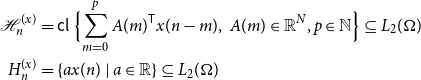 \begin{equation} \begin{aligned} \mathcal{H}_n^{(x)} &=\mathsf{cl\ } \Bigl \{\sum _{m = 0}^p A(m)^{\mathsf{T}} x(n-m), \ A(m) \in \mathbb{R}^N, p \in \mathbb{N} \Bigr \} \subseteq L_2(\Omega )\\ H_n^{(x)} &= \{a x(n)\ |\ a \in \mathbb{R}\} \subseteq L_2(\Omega ) \end{aligned} \end{equation}
where the closure is in mean-square. We will often omit the superscript $(x)$
, which should be clear from context. These spaces are separable, and as closed subspaces of a Hilbert space they are themselves Hilbert. We will denote the spaces generated in analogous ways by particular components of
$(x)$
, which should be clear from context. These spaces are separable, and as closed subspaces of a Hilbert space they are themselves Hilbert. We will denote the spaces generated in analogous ways by particular components of $x$
as, for example,
$x$
as, for example, $\mathcal{H}_n^{(i, j)}$
,
$\mathcal{H}_n^{(i, j)}$
, $\mathcal{H}_n^{(i)}$
or by all but a particular component as
$\mathcal{H}_n^{(i)}$
or by all but a particular component as $\mathcal{H}_n^{(-j)}$
.
$\mathcal{H}_n^{(-j)}$
.
From the Wold decomposition theorem (Lindquist & Picci, Reference Lindquist and Picci2015), every WSS sequence has the moving average $\mathsf{MA}(\infty )$
representation
$\mathsf{MA}(\infty )$
representation
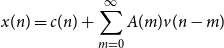 \begin{equation} x(n) = c(n) + \sum _{m = 0}^\infty A(m) v(n-m) \end{equation}
where $c(n)$
is a purely deterministic sequence,
$c(n)$
is a purely deterministic sequence, $v(n)$
is an uncorrelated sequence and
$v(n)$
is an uncorrelated sequence and $A(0) = I$
. We will assume that
$A(0) = I$
. We will assume that $c(n) = 0\ \forall n$
, which makes
$c(n) = 0\ \forall n$
, which makes $x(n)$
a regular non-deterministic sequence. This representation can be inverted (Lindquist & Picci, Reference Lindquist and Picci2015) to yield the Vector Autoregressive
$x(n)$
a regular non-deterministic sequence. This representation can be inverted (Lindquist & Picci, Reference Lindquist and Picci2015) to yield the Vector Autoregressive $\mathsf{VAR}(\infty )$
form
$\mathsf{VAR}(\infty )$
form
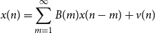 \begin{equation} x(n) = \sum _{m = 1}^\infty B(m) x(n-m) + v(n) \end{equation}
The Equations (2) and (3) can be represented as $x(n) = \mathsf{A}(z)v(n) = \mathsf{B}(z)x(n) + v(n)$
via the action of the operators
$x(n) = \mathsf{A}(z)v(n) = \mathsf{B}(z)x(n) + v(n)$
via the action of the operators
 \begin{equation*}\mathsf {A}(z) \;:\!=\; \sum _{m = 0}^\infty A(m)z^{-m}\end{equation*}
and
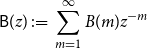 \begin{equation*}\mathsf {B}(z) \;:\!=\; \sum _{m = 1}^\infty B(m)z^{-m}\end{equation*}
where the operator $z^{-1}$
is the backshift operator acting on
$z^{-1}$
is the backshift operator acting on $\ell _2^N(\Omega )$
, the space of square summable sequences of
$\ell _2^N(\Omega )$
, the space of square summable sequences of $N$
-vectors having elements in
$N$
-vectors having elements in $L_2(\Omega )$
that is:
$L_2(\Omega )$
that is:
 \begin{equation} \mathsf{B}_{ij}(z)x_j(n) \;:\!=\; \sum _{m = 1}^\infty B_{ij}(m)x_j(n - m) \end{equation}
The operator $\mathsf{A}(z)$
contains only non-positive powers of
$\mathsf{A}(z)$
contains only non-positive powers of $z$
and is therefore called causal, and if
$z$
and is therefore called causal, and if $A(0) = 0$
then it is strictly causal. An operator containing only non-negative powers of
$A(0) = 0$
then it is strictly causal. An operator containing only non-negative powers of $z$
, for example,
$z$
, for example, $\mathsf{C}(z) = c_0 + c_1z + c_2z^2 + \cdots$
is anti-causal. These operators are often referred to as filters in signal processing, terminology which we often adopt as well.
$\mathsf{C}(z) = c_0 + c_1z + c_2z^2 + \cdots$
is anti-causal. These operators are often referred to as filters in signal processing, terminology which we often adopt as well.
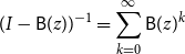
Finally, we have the well known inversion formula
 \begin{equation} \mathsf{A}(z) = (I - \mathsf{B}(z))^{-1} = \sum _{k = 0}^\infty \mathsf{B}(z)^k \end{equation}
The above assumptions are quite weak, and are essentially the minimal requirements needed to have a non-degenerate model. The strongest assumption we require is finally that $\Sigma _v$
is a diagonal and positive-definite matrix. Equivalently, the Wold decomposition could be written with
$\Sigma _v$
is a diagonal and positive-definite matrix. Equivalently, the Wold decomposition could be written with $A(0) \ne I$
and
$A(0) \ne I$
and $\Sigma _v = I$
, and we would be assuming that
$\Sigma _v = I$
, and we would be assuming that $A(0)$
is diagonal. This precludes the possibility of instantaneous causality (Granger, Reference Granger1969) or of processes being only weakly (as opposed to strongly) feedback free, in the terminology of Caines (Reference Caines1976). We formally state our setup as a definition:
$A(0)$
is diagonal. This precludes the possibility of instantaneous causality (Granger, Reference Granger1969) or of processes being only weakly (as opposed to strongly) feedback free, in the terminology of Caines (Reference Caines1976). We formally state our setup as a definition:
Definition 2.1 (Basic Setup). The process $x(n)$
is an
$x(n)$
is an $N$
dimensional, zero mean, wide-sense stationary process having invertible
$N$
dimensional, zero mean, wide-sense stationary process having invertible $\mathsf{VAR}(\infty )$
representation (3), where
$\mathsf{VAR}(\infty )$
representation (3), where $v(n)$
is sequentially uncorrelated and has a diagonal positive-definite covariance matrix. The
$v(n)$
is sequentially uncorrelated and has a diagonal positive-definite covariance matrix. The $\mathsf{MA}(\infty )$
representation of Equation (2) has
$\mathsf{MA}(\infty )$
representation of Equation (2) has $c(n) = 0\ \forall n$
and
$c(n) = 0\ \forall n$
and $A(0) = I$
.
$A(0) = I$
.
2.2 Granger causality
Definition 2.2 (Granger Causality). We will say that component $x_j$
Granger-causes component
$x_j$
Granger-causes component $x_i$
(with respect to
$x_i$
(with respect to $x$
) and write
$x$
) and write $x_j \overset{\text{GC}}{\rightarrow } x_i$
if
$x_j \overset{\text{GC}}{\rightarrow } x_i$
if
 \begin{equation}{\xi [{x_i(n)}\ |\ {\mathcal{H}_{n - 1}}]} \lt{\xi [{x_i(n)}\ |\ {\mathcal{H}^{(-j)}_{n - 1}}]} \end{equation}
where $\xi [x \ |\ \mathcal{H}] \;:\!=\; \mathbb{E} (x -{\hat{\mathbb{E}}[x\ |\ \mathcal{H}]})^2$
is the linear mean-squared estimation error and
$\xi [x \ |\ \mathcal{H}] \;:\!=\; \mathbb{E} (x -{\hat{\mathbb{E}}[x\ |\ \mathcal{H}]})^2$
is the linear mean-squared estimation error and
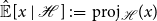 \begin{equation*}{\hat {\mathbb {E}}[x\ |\ \mathcal {H}]} \;:\!=\; \text {proj}_{\mathcal {H}}(x)\end{equation*}
denotes the (unique) projection onto the Hilbert space $\mathcal{H}$
.
$\mathcal{H}$
.
This notion captures the idea that the process $x_j$
provides information about
$x_j$
provides information about $x_i$
that is not available from elsewhere. The notion is closely related to the information theoretic measure of transfer entropy, indeed, if the distribution of
$x_i$
that is not available from elsewhere. The notion is closely related to the information theoretic measure of transfer entropy, indeed, if the distribution of $v(n)$
is known to be Gaussian then they are equivalent (Barnett et al., Reference Barnett, Barrett and Seth2009).
$v(n)$
is known to be Gaussian then they are equivalent (Barnett et al., Reference Barnett, Barrett and Seth2009).
The notion of conditional orthogonality is the essence of Granger causality, and enables us to obtain results for a fairly general class of WSS processes, rather than simply $\mathsf{VAR}(p)$
models.
$\mathsf{VAR}(p)$
models.
Definition 2.3 (Conditional Orthogonality). Consider three closed subspaces of a Hilbert space $\mathcal{A}$
,
$\mathcal{A}$
, $\mathcal{B}$
,
$\mathcal{B}$
, $\mathcal{X}$
. We say that
$\mathcal{X}$
. We say that $\mathcal{A}$
is conditionally orthogonal to
$\mathcal{A}$
is conditionally orthogonal to $\mathcal{B}$
given
$\mathcal{B}$
given $\mathcal{X}$
and write
$\mathcal{X}$
and write $\mathcal{A} \perp \mathcal{B}\ |\ \mathcal{X}$
if
$\mathcal{A} \perp \mathcal{B}\ |\ \mathcal{X}$
if
 \begin{equation*} \langle {a - {\hat {\mathbb {E}}[a\ |\ \mathcal {X}]}},{b - {\hat {\mathbb {E}}[b\ |\ \mathcal {X}]}}\rangle = 0\ \forall a \in \mathcal {A}, b \in \mathcal {B} \end{equation*}
An equivalent condition is that (see Lindquist & Picci (Reference Lindquist and Picci2015) Proposition 2.4.2)
 \begin{equation*} {\hat {\mathbb {E}}[\beta \ |\ {\mathcal {A} \vee \mathcal {X}}]} = {\hat {\mathbb {E}}[\beta \ |\ \mathcal {X}]}\ \forall \beta \in \mathcal {B} \end{equation*}
The following theorem captures a number of well known equivalent definitions or characterizations of Granger causality:
Theorem 2.1 (Granger Causality Equivalences). The following are equivalent:
-
(a) $x_j \overset{\text{GC}}{\nrightarrow } x_i$
-
(b)
$\forall m \in \mathbb{N}_+\ B_{ij}(m) = 0$
, that is,
$\mathsf{B}_{ij}(z) = 0$
-
(c)
$H_n^{(i)} \perp \mathcal{H}_{n-1}^{(j)}\ |\mathcal{H}_{n-1}^{(-j)}$
-
(d)
${\hat{\mathbb{E}}[{x_i(n)}\ |\ {\mathcal{H}_{n - 1}^{(-j)}}]} ={\hat{\mathbb{E}}[{x_i(n)}\ |\ {\mathcal{H}_{n - 1}}]}$


Proof.
These facts are quite well known. $(a) \Rightarrow (b)$
follows as a result of the uniqueness of orthogonal projection (i.e.,, the best estimate is necessarily the coefficients of the model).
$(a) \Rightarrow (b)$
follows as a result of the uniqueness of orthogonal projection (i.e.,, the best estimate is necessarily the coefficients of the model). $(b) \Rightarrow (c)$
follows since in computing
$(b) \Rightarrow (c)$
follows since in computing $(y -{\hat{\mathbb{E}}[y\ |\ {\mathcal{H}_{n - 1}^{(-j)}}]})$
for
$(y -{\hat{\mathbb{E}}[y\ |\ {\mathcal{H}_{n - 1}^{(-j)}}]})$
for $y \in H_n^{(i)}$
it is sufficient to consider
$y \in H_n^{(i)}$
it is sufficient to consider $y =x_i(n)$
by linearity, then since
$y =x_i(n)$
by linearity, then since $H_{n - 1}^{(i)} \subseteq \mathcal{H}_{n-1}^{(-j)}$
we have
$H_{n - 1}^{(i)} \subseteq \mathcal{H}_{n-1}^{(-j)}$
we have $(x_i(n) -{\hat{\mathbb{E}}[{x_i(n)}\ |\ {\mathcal{H}_{t - 1}^{(-j)}}]}) = v_i(n)$
since
$(x_i(n) -{\hat{\mathbb{E}}[{x_i(n)}\ |\ {\mathcal{H}_{t - 1}^{(-j)}}]}) = v_i(n)$
since $\mathsf{B}_{ij}(z) = 0$
. The result follows since
$\mathsf{B}_{ij}(z) = 0$
. The result follows since $v_i(n) \perp \mathcal{H}_{n-1}$
.
$v_i(n) \perp \mathcal{H}_{n-1}$
. $(c) \iff (d)$
is a result of the equivalence in Definition 2.3. And,
$(c) \iff (d)$
is a result of the equivalence in Definition 2.3. And, $(d) \implies (a)$
follows directly from the Definition.
$(d) \implies (a)$
follows directly from the Definition.
2.3 Granger causality graphs
We establish some graph theoretic notation and terminology, collected formally in definitions for the reader’s convenient reference.
Definition 2.4 (Graph Theory Review). A graph $\mathcal{G} = (V, \mathcal{E})$
is a tuple of sets respectively called nodes and edges. Throughout this paper, we have in all cases
$\mathcal{G} = (V, \mathcal{E})$
is a tuple of sets respectively called nodes and edges. Throughout this paper, we have in all cases $V = [N] \;:\!=\; \{1, 2, \ldots, N\}$
. We will also focus solely on directed graphs, where the edges
$V = [N] \;:\!=\; \{1, 2, \ldots, N\}$
. We will also focus solely on directed graphs, where the edges $\mathcal{E} \subseteq V \times V$
are ordered pairs.
$\mathcal{E} \subseteq V \times V$
are ordered pairs.
A (directed) path (of length $r$
) from node
$r$
) from node $i$
to node
$i$
to node $j$
, denoted
$j$
, denoted $i \rightarrow \cdots \rightarrow j$
, is a sequence
$i \rightarrow \cdots \rightarrow j$
, is a sequence $a_0, a_1, \ldots, a_{r - 1}, a_r$
with
$a_0, a_1, \ldots, a_{r - 1}, a_r$
with $a_0 = i$
and
$a_0 = i$
and $a_r = j$
such that
$a_r = j$
such that $\forall \ 0 \le k \le r\ (a_k, a_{k + 1}) \in \mathcal{E}$
, and where
$\forall \ 0 \le k \le r\ (a_k, a_{k + 1}) \in \mathcal{E}$
, and where $(a_k, a_{k - 1})$
are distinct for
$(a_k, a_{k - 1})$
are distinct for $0 \le k \lt r$
.
$0 \le k \lt r$
.
A cycle is a path of length $2$
or more between a node and itself. An edge between a node and itself
$2$
or more between a node and itself. An edge between a node and itself $(i, i) \in \mathcal{E}$
(which we do not consider to be a cycle) is referred to as a loop.
$(i, i) \in \mathcal{E}$
(which we do not consider to be a cycle) is referred to as a loop.
A graph $\mathcal{G}$
is a directed acyclic graph (DAG) if it is a directed graph and does not contain any cycles.
$\mathcal{G}$
is a directed acyclic graph (DAG) if it is a directed graph and does not contain any cycles.
Definition 2.5 (Parents, Grandparents, Ancestors). A node $j$
is a parent of node
$j$
is a parent of node $i$
if
$i$
if $(j, i) \in \mathcal{E}$
. The set of all
$(j, i) \in \mathcal{E}$
. The set of all $i$
’s parents will be denoted
$i$
’s parents will be denoted $pa(i)$
, and we explicitly exclude loops as a special case, that is,
$pa(i)$
, and we explicitly exclude loops as a special case, that is, $i \not \in{pa(i)}$
even if
$i \not \in{pa(i)}$
even if $(i, i) \in \mathcal{E}$
.
$(i, i) \in \mathcal{E}$
.
The set of level $\ell$
grandparents of node
$\ell$
grandparents of node $i$
, denoted
$i$
, denoted $gp_{\ell }({i})$
, is the set such that
$gp_{\ell }({i})$
, is the set such that $j \in{gp_{\ell }({i})}$
if and only if there is a directed path of length
$j \in{gp_{\ell }({i})}$
if and only if there is a directed path of length $\ell$
in
$\ell$
in $\mathcal{G}$
from
$\mathcal{G}$
from $j$
to
$j$
to $i$
. Clearly,
$i$
. Clearly, ${pa(i)} ={gp_{1}({i})}$
.
${pa(i)} ={gp_{1}({i})}$
.
Finally, the set of level $\ell$
ancestors of
$\ell$
ancestors of $i$
:
$i$
: ${\mathcal{A}_{\ell }({i})} = \bigcup _{\lambda \le \ell }{gp_{\lambda }({i})}$
is the set such that
${\mathcal{A}_{\ell }({i})} = \bigcup _{\lambda \le \ell }{gp_{\lambda }({i})}$
is the set such that $j \in{\mathcal{A}_{\ell }({i})}$
if and only if there is a directed path of length
$j \in{\mathcal{A}_{\ell }({i})}$
if and only if there is a directed path of length $\ell$
or less in
$\ell$
or less in $\mathcal{G}$
from
$\mathcal{G}$
from $j$
to
$j$
to $i$
. The set of all ancestors of
$i$
. The set of all ancestors of $i$
(i.e.,
$i$
(i.e., $\mathcal{A}_{N}({i})$
) is denoted simply
$\mathcal{A}_{N}({i})$
) is denoted simply $\mathcal{A}({i})$
.
$\mathcal{A}({i})$
.
Recall that we do not allow a node to be its own parent, but unless $\mathcal{G}$
is a DAG, a node can be its own ancestor. We will occasionally need to explicitly exclude
$\mathcal{G}$
is a DAG, a node can be its own ancestor. We will occasionally need to explicitly exclude $i$
from
$i$
from $\mathcal{A}({i})$
, in which case we will write
$\mathcal{A}({i})$
, in which case we will write ${\mathcal{A}({i})}\setminus \{i\}$
.
${\mathcal{A}({i})}\setminus \{i\}$
.
Our principal object of study will be a graph determined by Granger causality relations as follows.
Definition 2.6 (Causality graph). We define the Granger causality graph $\mathcal{G} = ([N], \mathcal{E})$
to be the directed graph formed on
$\mathcal{G} = ([N], \mathcal{E})$
to be the directed graph formed on $N$
vertices where an edge
$N$
vertices where an edge $(j, i) \in \mathcal{E}$
if and only if
$(j, i) \in \mathcal{E}$
if and only if $x_j$
Granger-causes
$x_j$
Granger-causes $x_i$
(with respect to
$x_i$
(with respect to $x$
). That is,
$x$
). That is,
 \begin{equation*}(j, i) \in \mathcal {E} \iff j \in {pa(i)} \iff x_j \overset {\text {GC}}{\rightarrow } x_i\end{equation*}
The edges of the Granger causality graph $\mathcal{G}$
can be given a general notion of “weight” by associating an edge
$\mathcal{G}$
can be given a general notion of “weight” by associating an edge $(j, i)$
with the strictly causal operator
$(j, i)$
with the strictly causal operator $\mathsf{B}_{ij}(z)$
(see Equation (4)). Hence, the matrix
$\mathsf{B}_{ij}(z)$
(see Equation (4)). Hence, the matrix $\mathsf{B}(z)$
is analogous to a weighted adjacency matrix Footnote 1 for the graph
$\mathsf{B}(z)$
is analogous to a weighted adjacency matrix Footnote 1 for the graph $\mathcal{G}$
. And, in the same way that the
$\mathcal{G}$
. And, in the same way that the $k^{\text{th}}$
power of an adjacency matrix counts the number of paths of length
$k^{\text{th}}$
power of an adjacency matrix counts the number of paths of length $k$
between nodes,
$k$
between nodes, $(\mathsf{B}(z)^k)_{ij}$
is a filter isolating the “action” of
$(\mathsf{B}(z)^k)_{ij}$
is a filter isolating the “action” of $j$
on
$j$
on $i$
at a time lag of
$i$
at a time lag of $k$
steps, this is exemplified in the inversion formula (5).
$k$
steps, this is exemplified in the inversion formula (5).
From the $\mathsf{VAR}$
representation of
$\mathsf{VAR}$
representation of $x(n)$
there is clearly a close relationship between each node and its parent nodes, the relationship is quantified through the sparsity pattern of
$x(n)$
there is clearly a close relationship between each node and its parent nodes, the relationship is quantified through the sparsity pattern of $\mathsf{B}(z)$
. The work of Caines & Chan (Reference Caines and Chan1975) starts by defining causality (including between groups of processes) via the notion of feedback free processes in terms of
$\mathsf{B}(z)$
. The work of Caines & Chan (Reference Caines and Chan1975) starts by defining causality (including between groups of processes) via the notion of feedback free processes in terms of $\mathsf{A}(z)$
. The following proposition provides a similar interpretation of the sparsity pattern of
$\mathsf{A}(z)$
. The following proposition provides a similar interpretation of the sparsity pattern of $A(z)$
in terms of the causality graph
$A(z)$
in terms of the causality graph $\mathcal{G}$
.
$\mathcal{G}$
.
Proposition 2.1 (Ancestor Expansion). The component $x_i(n)$
of
$x_i(n)$
of $x(n)$
can be represented in terms of its parents in
$x(n)$
can be represented in terms of its parents in $\mathcal{G}$
:
$\mathcal{G}$
:
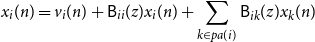 \begin{equation} x_i(n) = v_i(n) + \mathsf{B}_{ii}(z)x_i(n) + \sum _{k \in{pa(i)}}\mathsf{B}_{ik}(z)x_k(n) \end{equation}
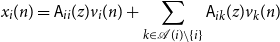
Moreover, $x_i(\cdot )$
can be expanded in terms of its ancestor’s
$x_i(\cdot )$
can be expanded in terms of its ancestor’s $v(n)$
components only:
$v(n)$
components only:
 \begin{equation} x_i(n) = \mathsf{A}_{ii}(z)v_i(n) + \sum _{k \in{\mathcal{A}({i})} \setminus \{i\}}\mathsf{A}_{ik}(z)v_k(n) \end{equation}
where $\mathsf{A}(z) = \sum _{m = 0}^\infty A(m)z^{-m}$
is the filter from the Wold decomposition representation of
$\mathsf{A}(z) = \sum _{m = 0}^\infty A(m)z^{-m}$
is the filter from the Wold decomposition representation of $x(n)$
, Equation (2).
$x(n)$
, Equation (2).
Proof.
Equation (7) is immediate from the $\mathsf{VAR}(\infty )$
representation of Equation (3) and Theorem 2.1, we are left to demonstrate (8).
$\mathsf{VAR}(\infty )$
representation of Equation (3) and Theorem 2.1, we are left to demonstrate (8).
From Equation (3), which we are assuming throughout the paper to be invertible, we can write
 \begin{equation*} x(n) = (I - \mathsf {B}(z))^{-1} v(n) \end{equation*}
where necessarily $(I - \mathsf{B}(z))^{-1} = \mathsf{A}(z)$
due to the uniqueness of the Wold decomposition. Since
$(I - \mathsf{B}(z))^{-1} = \mathsf{A}(z)$
due to the uniqueness of the Wold decomposition. Since $\mathsf{B}(z)$
is stable we have
$\mathsf{B}(z)$
is stable we have
 \begin{equation} (I - \mathsf{B}(z))^{-1} = \sum _{k = 0}^\infty \mathsf{B}(z)^k \end{equation}
Invoking the Cayley-Hamilton theorem allows writing the infinite sum of (9) in terms of finite powers of $\mathsf{B}$
.
$\mathsf{B}$
.
Let $S$
be a matrix with elements in
$S$
be a matrix with elements in $\{0, 1\}$
which represents the sparsity pattern of
$\{0, 1\}$
which represents the sparsity pattern of $\mathsf{B}(z)$
, from Lemma D.1
$\mathsf{B}(z)$
, from Lemma D.1 $S$
is the transpose of the adjacency matrix for
$S$
is the transpose of the adjacency matrix for $\mathcal{G}$
and hence
$\mathcal{G}$
and hence $(S^k)_{ij}$
is non-zero if and only if
$(S^k)_{ij}$
is non-zero if and only if $j \in{gp_{k}({i})}$
, and therefore
$j \in{gp_{k}({i})}$
, and therefore $\mathsf{B}(z)^k_{ij} = 0$
if
$\mathsf{B}(z)^k_{ij} = 0$
if $j \not \in{gp_{k}({i})}$
. Finally, since
$j \not \in{gp_{k}({i})}$
. Finally, since ${\mathcal{A}({i})} = \bigcup _{k = 1}^N{gp_{k}({i})}$
we see that
${\mathcal{A}({i})} = \bigcup _{k = 1}^N{gp_{k}({i})}$
we see that $\mathsf{A}_{ij}(z)$
is zero if
$\mathsf{A}_{ij}(z)$
is zero if $j \not \in{\mathcal{A}({i})}$
.
$j \not \in{\mathcal{A}({i})}$
.
Therefore
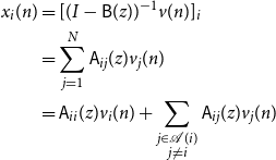 \begin{align*} x_i(n) &= [(I - \mathsf{B}(z))^{-1}v(n)]_i\\ &= \sum _{j = 1}^N \mathsf{A}_{ij}(z) v_j(n)\\ &= \mathsf{A}_{ii}(z) v_i(n) + \sum _{\substack{j \in{\mathcal{A}({i})} \\ j \ne i}} \mathsf{A}_{ij}(z) v_j(n) \end{align*}
This completes the proof.
Proposition 2.1 is ultimately about the sparsity pattern in the Wold decomposition matrices $A(m)$
since
$A(m)$
since $x_i(n) = \sum _{m = 0}^\infty \sum _{j = 1}^N A_{ij}(m)v_j(n - m)$
. The proposition states that if
$x_i(n) = \sum _{m = 0}^\infty \sum _{j = 1}^N A_{ij}(m)v_j(n - m)$
. The proposition states that if $j \not \in{\mathcal{A}({i})}$
, then
$j \not \in{\mathcal{A}({i})}$
, then $\mathsf{A}_{ij}(z) = 0$
.
$\mathsf{A}_{ij}(z) = 0$
.
2.4 Pairwise granger causality
Recall that Granger causality in general must be understood with respect to a particular universe of observations. If $x_j \overset{\text{GC}}{\rightarrow } x_i$
with respect to
$x_j \overset{\text{GC}}{\rightarrow } x_i$
with respect to $x_{-k}$
, it may not hold with respect to
$x_{-k}$
, it may not hold with respect to $x$
. For example,
$x$
. For example, $x_k$
may be a common ancestor which when observed, completely explains the connection from
$x_k$
may be a common ancestor which when observed, completely explains the connection from $x_j$
to
$x_j$
to $x_i$
. In this section we study pairwise Granger causality, and seek to understand when knowledge of pairwise relations is sufficient to deduce the fully conditional relations of
$x_i$
. In this section we study pairwise Granger causality, and seek to understand when knowledge of pairwise relations is sufficient to deduce the fully conditional relations of $\mathcal{G}$
.
$\mathcal{G}$
.
Definition 2.7 (Pairwise Granger causality). We will say that $x_j$
pairwise Granger-causes
$x_j$
pairwise Granger-causes $x_i$
and write
$x_i$
and write $x_j \overset{\text{PW}}{\rightarrow } x_i$
if
$x_j \overset{\text{PW}}{\rightarrow } x_i$
if $x_j$
Granger-causes
$x_j$
Granger-causes $x_i$
with respect only to
$x_i$
with respect only to $(x_i, x_j)$
.
$(x_i, x_j)$
.
This notion is of interest for a variety of reasons. From a purely conceptual standpoint, we will see how the notion can in some sense capture the idea of “flow of information” in the underlying graph, in the sense that if $j \in{\mathcal{A}({i})}$
we expect that
$j \in{\mathcal{A}({i})}$
we expect that $j \overset{\text{PW}}{\rightarrow } i$
. It may also be useful for reasoning about the conditions under which unobserved components of
$j \overset{\text{PW}}{\rightarrow } i$
. It may also be useful for reasoning about the conditions under which unobserved components of $x(n)$
may or may not interfere with inference in the actually observed components. Finally, motivated from a practical standpoint to analyze causation in large systems, practical estimation procedures based purely on pairwise causality tests are of interest since the computation of such pairwise relations is substantially easier than the full conditional relations.
$x(n)$
may or may not interfere with inference in the actually observed components. Finally, motivated from a practical standpoint to analyze causation in large systems, practical estimation procedures based purely on pairwise causality tests are of interest since the computation of such pairwise relations is substantially easier than the full conditional relations.
The following propositions are essentially lemmas used for the proof of the upcoming Proposition 2.4, but remain relevant for providing intuitive insight into the problems at hand.
Proposition 2.2 (Fully Disjointed Nodes; Proof in Section D.2). Consider distinct nodes $i, j$
in a Granger causality graph
$i, j$
in a Granger causality graph $\mathcal{G}$
. If
$\mathcal{G}$
. If
-
(a)
$j \not \in{\mathcal{A}({i})}$
and
$i \not \in{\mathcal{A}({j})}$
-
(b)
${\mathcal{A}({i})}\cap{\mathcal{A}({j})} = \emptyset$


then $\mathcal{H}_n^{(i)} \perp \mathcal{H}_n^{(j)}$
, that is,
$\mathcal{H}_n^{(i)} \perp \mathcal{H}_n^{(j)}$
, that is, $\forall l, m \in \mathbb{Z}_+\ \mathbb{E}[x_i(n - l)x_j(n - m)] = 0$
. Moreover, this means that
$\forall l, m \in \mathbb{Z}_+\ \mathbb{E}[x_i(n - l)x_j(n - m)] = 0$
. Moreover, this means that $j \overset{\text{PW}}{\nrightarrow } i$
and
$j \overset{\text{PW}}{\nrightarrow } i$
and ${\hat{\mathbb{E}}[{x_j(n)}\ |\ {\mathcal{H}_n^{(i)}}]} = 0$
.
${\hat{\mathbb{E}}[{x_j(n)}\ |\ {\mathcal{H}_n^{(i)}}]} = 0$
.
Remark 2.1. It is possible for components of $x(n)$
to be correlated at some time lags without resulting in pairwise causality. For instance, the conclusion
$x(n)$
to be correlated at some time lags without resulting in pairwise causality. For instance, the conclusion $j \overset{\text{PW}}{\nrightarrow } i$
of Proposition 2.2 will still hold even if
$j \overset{\text{PW}}{\nrightarrow } i$
of Proposition 2.2 will still hold even if $i \in{\mathcal{A}({j})}$
, since
$i \in{\mathcal{A}({j})}$
, since $j$
cannot provide any information about
$j$
cannot provide any information about $i$
that is not available from observing
$i$
that is not available from observing $i$
itself.
$i$
itself.
Proposition 2.3 (Not an Ancestor, No Common Cause; Proof in Appendix D.2). Consider distinct nodes $i, j$
in a Granger causality graph
$i, j$
in a Granger causality graph $\mathcal{G}$
. If
$\mathcal{G}$
. If
-
(a)
$j \not \in{\mathcal{A}({i})}$
-
(b)
${\mathcal{A}({i})}\cap{\mathcal{A}({j})} = \emptyset$


then $j \overset{\text{PW}}{\nrightarrow } i$
.
$j \overset{\text{PW}}{\nrightarrow } i$
.
The previous result can still be strengthened significantly; notice that it is possible to have some $k \in{\mathcal{A}({i})} \cap{\mathcal{A}({j})}$
where still
$k \in{\mathcal{A}({i})} \cap{\mathcal{A}({j})}$
where still $j \overset{\text{PW}}{\nrightarrow } i$
, an example is furnished by the three node graph
$j \overset{\text{PW}}{\nrightarrow } i$
, an example is furnished by the three node graph $k \rightarrow i \rightarrow j$
where clearly
$k \rightarrow i \rightarrow j$
where clearly $k \in{\mathcal{A}({i})}\cap{\mathcal{A}({j})}$
but
$k \in{\mathcal{A}({i})}\cap{\mathcal{A}({j})}$
but $j \overset{\text{PW}}{\nrightarrow } i$
. We must introduce the concept of a confounding variable, which effectively eliminates the possibility presented in this example.
$j \overset{\text{PW}}{\nrightarrow } i$
. We must introduce the concept of a confounding variable, which effectively eliminates the possibility presented in this example.
Definition 2.8 (Confounder). A node $k$
will be referred to as a confounder of nodes
$k$
will be referred to as a confounder of nodes $i, j$
(neither of which are equal to
$i, j$
(neither of which are equal to $k$
) if
$k$
) if $k \in{\mathcal{A}({i})} \cap{\mathcal{A}({j})}$
and there exists a path
$k \in{\mathcal{A}({i})} \cap{\mathcal{A}({j})}$
and there exists a path $k \rightarrow \cdots \rightarrow i$
not containing
$k \rightarrow \cdots \rightarrow i$
not containing $j$
, and a path
$j$
, and a path $k \rightarrow \cdots \rightarrow j$
not containing
$k \rightarrow \cdots \rightarrow j$
not containing $i$
. A simple example is furnished by the “fork” graph
$i$
. A simple example is furnished by the “fork” graph $i \leftarrow k \rightarrow j$
.
$i \leftarrow k \rightarrow j$
.
A similar proposition as the following also appears as [Datta-Gupta, (Reference Datta-Gupta and Mazumdar2014), Prop. 5.3.2]:
Proposition 2.4 (Necessary Conditions). If in a Granger causality graph $\mathcal{G}$
where
$\mathcal{G}$
where $j \overset{\text{PW}}{\rightarrow } i$
then
$j \overset{\text{PW}}{\rightarrow } i$
then $j \in{\mathcal{A}({i})}$
or
$j \in{\mathcal{A}({i})}$
or $\exists k \in{\mathcal{A}({i})} \cap{\mathcal{A}({j})}$
which is a confounder of
$\exists k \in{\mathcal{A}({i})} \cap{\mathcal{A}({j})}$
which is a confounder of $(i, j)$
.
$(i, j)$
.
Proof.
The proof is by way of contradiction. To this end, suppose that $j$
is a node such that:
$j$
is a node such that:
-
(a)
$j \not \in{\mathcal{A}({i})}$
-
(b) every
$k \in{\mathcal{A}({i})} \cap{\mathcal{A}({j})}$
every
$k \rightarrow \cdots \rightarrow j$
path contains
$i$
.


Firstly, notice that every $u \in \big ({pa(j)} \setminus \{i\}\big )$
necessarily inherits these same two properties. This follows since if we also had
$u \in \big ({pa(j)} \setminus \{i\}\big )$
necessarily inherits these same two properties. This follows since if we also had $u \in{\mathcal{A}({i})}$
then
$u \in{\mathcal{A}({i})}$
then $u \in{\mathcal{A}({i})} \cap{\mathcal{A}({j})}$
so by our assumption every
$u \in{\mathcal{A}({i})} \cap{\mathcal{A}({j})}$
so by our assumption every $u \rightarrow \cdots \rightarrow j$
path must contain
$u \rightarrow \cdots \rightarrow j$
path must contain $i$
, but
$i$
, but $u \in{pa(j)}$
so
$u \in{pa(j)}$
so $u \rightarrow j$
is a path that doesn’t contain
$u \rightarrow j$
is a path that doesn’t contain $i$
, and therefore
$i$
, and therefore $u \not \in{\mathcal{A}({i})}$
; moreover, if we consider
$u \not \in{\mathcal{A}({i})}$
; moreover, if we consider $w \in{\mathcal{A}({i})} \cap{\mathcal{A}({u})}$
then we also have
$w \in{\mathcal{A}({i})} \cap{\mathcal{A}({u})}$
then we also have $w \in{\mathcal{A}({i})} \cap{\mathcal{A}({j})}$
so the assumption implies that every
$w \in{\mathcal{A}({i})} \cap{\mathcal{A}({j})}$
so the assumption implies that every $w \rightarrow \cdots \rightarrow j$
path must contain
$w \rightarrow \cdots \rightarrow j$
path must contain $i$
. These properties therefore extend inductively to every
$i$
. These properties therefore extend inductively to every $u \in \big ({\mathcal{A}({j})} \setminus \{i\}\big )$
.
$u \in \big ({\mathcal{A}({j})} \setminus \{i\}\big )$
.
In order to deploy a recursive argument, define the following partition of $pa(u)$
, for some node
$pa(u)$
, for some node $u$
:
$u$
:
 \begin{align*} C_0(u) &= \{k \in{pa(u)}\ |\ i \not \in{\mathcal{A}({k})},{\mathcal{A}({i})} \cap{\mathcal{A}({k})} = \emptyset, k \ne i\}\\ C_1(u) &= \{k \in{pa(u)}\ |\ i \in{\mathcal{A}({k})} \text{ or } k = i\}\\ C_2(u) &= \{k \in{pa(u)}\ |\ i \not \in{\mathcal{A}({k})},{\mathcal{A}({i})} \cap{\mathcal{A}({k})} \ne \emptyset, k \ne i\} \end{align*}
We notice that for any $u$
having the properties
$u$
having the properties $(a), (b)$
above, we must have
$(a), (b)$
above, we must have $C_2(u) = \emptyset$
since if
$C_2(u) = \emptyset$
since if $k \in C_2(u)$
then
$k \in C_2(u)$
then $\exists w \in{\mathcal{A}({i})} \cap{\mathcal{A}({k})}$
(and
$\exists w \in{\mathcal{A}({i})} \cap{\mathcal{A}({k})}$
(and $w \in{\mathcal{A}({i})} \cap{\mathcal{A}({u})}$
, since
$w \in{\mathcal{A}({i})} \cap{\mathcal{A}({u})}$
, since $k \in{pa(u)}$
) such that
$k \in{pa(u)}$
) such that $i \not \in{\mathcal{A}({k})}$
and therefore there must be a path
$i \not \in{\mathcal{A}({k})}$
and therefore there must be a path ${w \rightarrow \cdots \rightarrow k}\rightarrow u$
which does not contain
${w \rightarrow \cdots \rightarrow k}\rightarrow u$
which does not contain $i$
, contradicting property
$i$
, contradicting property $(b)$
. Moreover, for any
$(b)$
. Moreover, for any $u \in \big ({\mathcal{A}({j})} \setminus \{i\}\big )$
and
$u \in \big ({\mathcal{A}({j})} \setminus \{i\}\big )$
and $k \in C_0(u)$
, Proposition 2.3 shows that
$k \in C_0(u)$
, Proposition 2.3 shows that $H_n^{(i)} \perp \mathcal{H}_{n-1}^{(j)} |\mathcal{H}_{n-1}^{(i)}$
.
$H_n^{(i)} \perp \mathcal{H}_{n-1}^{(j)} |\mathcal{H}_{n-1}^{(i)}$
.
In order to establish $j \overset{\text{PW}}{\nrightarrow } i$
, choose an arbitrary element of
$j \overset{\text{PW}}{\nrightarrow } i$
, choose an arbitrary element of $\mathcal{H}_{t - 1}^{(j)}$
and represent it via the action of a strictly causal filter
$\mathcal{H}_{t - 1}^{(j)}$
and represent it via the action of a strictly causal filter $\Phi (z)$
, that is,
$\Phi (z)$
, that is, $\Phi (z) x_j(n) \in \mathcal{H}_{n-1}^{(j)}$
, by Theorem 2.1 it suffices to show that
$\Phi (z) x_j(n) \in \mathcal{H}_{n-1}^{(j)}$
, by Theorem 2.1 it suffices to show that
 \begin{equation} \langle{x_i(n)},{\Phi (z)x_j(n) -{\hat{\mathbb{E}}[{\Phi (z)x_j(n)}\ |\ {\mathcal{H}_{t - 1}^{(i)}}]}}\rangle = 0 \end{equation}
Denote $e_j \;:\!=\; e_j^{S(j)}$
, we can write
$e_j \;:\!=\; e_j^{S(j)}$
, we can write $x_j(n) = e_j^{\mathsf{T}} x_{S(j)}(n)$
, and therefore from Equation (D3) there exist strictly causal filters
$x_j(n) = e_j^{\mathsf{T}} x_{S(j)}(n)$
, and therefore from Equation (D3) there exist strictly causal filters $\Gamma _s(z)$
and
$\Gamma _s(z)$
and $\Lambda _{sk}(z)$
(defined for ease of notation) such that
$\Lambda _{sk}(z)$
(defined for ease of notation) such that
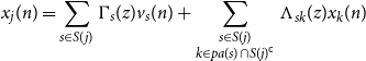 \begin{equation*} x_j(n) = \sum _{s \in S(j)} \Gamma _s(z)v_s(n) + \sum _{\substack {s \in S(j) \\ k \in {pa(s)} \cap S(j)^{\mathsf {c}}}} \Lambda _{sk}(z)x_k(n) \end{equation*}
When we substitute this expression into the left hand side of Equation (10), we may cancel each term involving $v_s$
by Lemma D.2, and each
$v_s$
by Lemma D.2, and each $k \in C_0(s)$
by our earlier argument, leaving us with
$k \in C_0(s)$
by our earlier argument, leaving us with
 \begin{equation*} \sum _{\substack {s \in S(j) \\ k \in C_1(s) \cap S(j)^{\mathsf {c}}}}\langle {x_i(n)},{\Phi (z)\Lambda _{sk}(z)x_k(n) - {\hat {\mathbb {E}}[{\Phi (z)\Lambda _{sk}(z)x_k(n)}\ |\ {\mathcal {H}_{t - 1}^{(i)}}]}}\rangle \end{equation*}
Since each $k \in C_1(s)$
with
$k \in C_1(s)$
with $k \ne i$
inherits properties
$k \ne i$
inherits properties $(a)$
and
$(a)$
and $(b)$
above, we can recursively expand each
$(b)$
above, we can recursively expand each $x_k$
of the above summation until reaching
$x_k$
of the above summation until reaching $k = i$
(which is guaranteed to terminate due to the definition of
$k = i$
(which is guaranteed to terminate due to the definition of $C_1(u)$
) which leaves us with some strictly causal filter
$C_1(u)$
) which leaves us with some strictly causal filter $F(z)$
such that the left hand side of Equation (10) is equal to
$F(z)$
such that the left hand side of Equation (10) is equal to
 \begin{equation*} \langle {x_i(n)},{\Phi (z)F(z)x_i(n) - {\hat {\mathbb {E}}[{\Phi (z)F(z)x_i(n)}\ |\ {\mathcal {H}_{t - 1}^{(i)}}]}}\rangle \end{equation*}
and this is $0$
since
$0$
since $\Phi (z)F(z)x_i(n) \in \mathcal{H}_{n-1}^{(i)}$
.
$\Phi (z)F(z)x_i(n) \in \mathcal{H}_{n-1}^{(i)}$
.
Remark 2.2. The interpretation of this proposition is that for $j \overset{\text{PW}}{\rightarrow } i$
then there must either be “causal flow” from
$j \overset{\text{PW}}{\rightarrow } i$
then there must either be “causal flow” from $j$
to
$j$
to $i$
(
$i$
( $j \in{\mathcal{A}({i})}$
) or there must be a confounder
$j \in{\mathcal{A}({i})}$
) or there must be a confounder $k$
through which common information is received.
$k$
through which common information is received.
An interesting corollary is the following:
Corollary 2.1.
If the graph $\mathcal{G}$
is a DAG then
$\mathcal{G}$
is a DAG then $j \overset{\text{PW}}{\rightarrow } i, i \overset{\text{PW}}{\rightarrow } j \implies \exists k \in{\mathcal{A}({i})} \cap{\mathcal{A}({j})}$
confounding
$j \overset{\text{PW}}{\rightarrow } i, i \overset{\text{PW}}{\rightarrow } j \implies \exists k \in{\mathcal{A}({i})} \cap{\mathcal{A}({j})}$
confounding $(i, j)$
.
$(i, j)$
.
It seems reasonable to expect a converse of Proposition 2.4 to hold, that is, $j \in{\mathcal{A}({i})} \Rightarrow j \overset{\text{PW}}{\rightarrow } i$
. Unfortunately, this is not the case in general, as different paths through
$j \in{\mathcal{A}({i})} \Rightarrow j \overset{\text{PW}}{\rightarrow } i$
. Unfortunately, this is not the case in general, as different paths through $\mathcal{G}$
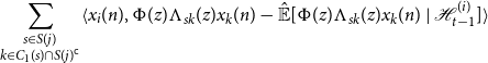
can lead to cancelation (see Figure 1(a)). In fact, we do not even have
$\mathcal{G}$
can lead to cancelation (see Figure 1(a)). In fact, we do not even have $j \in{pa(i)} \Rightarrow j \overset{\text{PW}}{\rightarrow } i$
(see Figure 1(b)).
$j \in{pa(i)} \Rightarrow j \overset{\text{PW}}{\rightarrow } i$
(see Figure 1(b)).
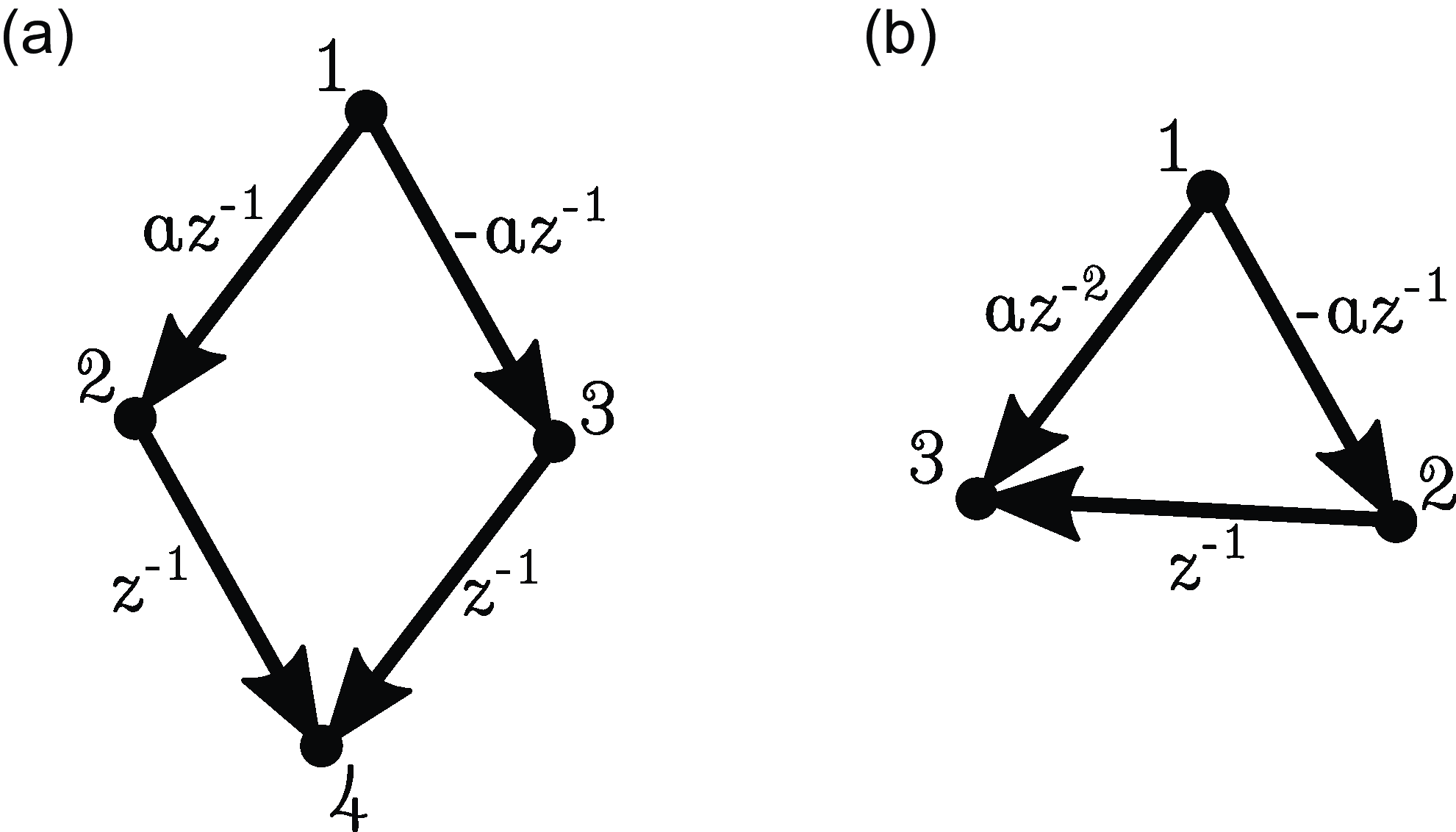
Figure 1. Examples illustrating the difficulty of obtaining a converse to Proposition 2.4. (a) Path cancelation: $j \in{\mathcal{A}({i})} \nRightarrow j \overset{\text{PW}}{\rightarrow } i$
. (b) Cancellation from time lag:
$j \in{\mathcal{A}({i})} \nRightarrow j \overset{\text{PW}}{\rightarrow } i$
. (b) Cancellation from time lag: $j \in{pa(i)} \nRightarrow j \overset{\text{PW}}{\rightarrow } i$
.
$j \in{pa(i)} \nRightarrow j \overset{\text{PW}}{\rightarrow } i$
.
2.5 Strongly causal graphs
In this section and the next we will seek to understand when converse statements of Proposition 2.4 do hold. One possibility is to restrict the coefficients of the system matrix, for example, by requiring that $B_{ij}(m) \ge 0$
. Instead, we think it more meaningful to focus on the defining feature of time series networks, that is, the topology of
$B_{ij}(m) \ge 0$
. Instead, we think it more meaningful to focus on the defining feature of time series networks, that is, the topology of $\mathcal{G}$
. To this end, we introduce the following notion of a strongly causal graph (SCG).
$\mathcal{G}$
. To this end, we introduce the following notion of a strongly causal graph (SCG).
Definition 2.9 (Strongly Causal). We will say that a Granger causality graph $\mathcal{G}$
is strongly causal if there is at most one directed path between any two nodes. That is, if the graph is a polytree. Strongly Causal Graphs will be referred to as SCGs.
$\mathcal{G}$
is strongly causal if there is at most one directed path between any two nodes. That is, if the graph is a polytree. Strongly Causal Graphs will be referred to as SCGs.
Examples of strongly causal graphs include directed trees (or forests), the diamond shaped graph containing $i \rightarrow j \leftarrow k$
and
$i \rightarrow j \leftarrow k$
and $i \rightarrow j' \leftarrow k$
, and Figure 4 of this paper. Importantly, a maximally connected bipartite graph with
$i \rightarrow j' \leftarrow k$
, and Figure 4 of this paper. Importantly, a maximally connected bipartite graph with $2N$
nodes is also strongly causal, demonstrating both that the number of edges of such a graph can still scale quadratically with the number of nodes. It is evident that the strong causal property is inherited by subgraphs.
$2N$
nodes is also strongly causal, demonstrating both that the number of edges of such a graph can still scale quadratically with the number of nodes. It is evident that the strong causal property is inherited by subgraphs.
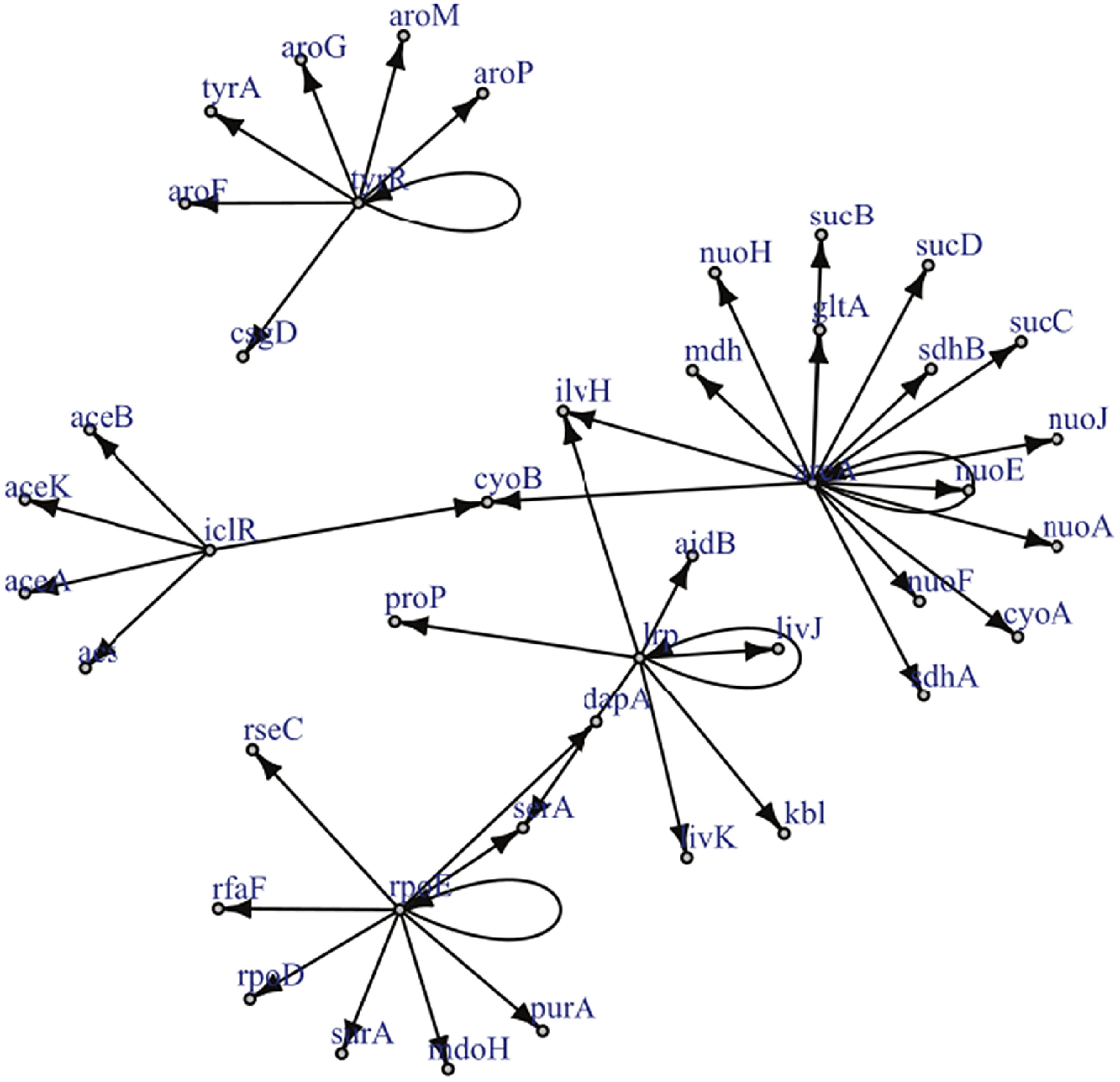
Figure 2. Reproduced under the creative commons attribution non-commercial license (http://creativecommons.org/licenses/by-nc/2.5) is a known gene regulatory network for a certain strain of E.Coli. The graph has only a single edge violating strong causality.
Example 2.1. Though examples of SCGs are easy to construct in theory, should practitioners expect SCGs to arise in application? While a positive answer to this question is not necessary for the concept to be useful, it is certainly sufficient. Though the answer is likely to depend upon the particular application area, examples appear to be available in biology, in particular, the authors of Shojaie & Michailidis (Reference Shojaie and Michailidis2010) cite an example of the so called “transcription regulatory network of E.coli” (reproduced in Figure 2), and Ma et al. (Reference Ma, Kemmeren, Gresham and Statnikov2014) study a much larger regulatory network of Saccharomyces cerevisiae. These networks, which we reproduce in Figure 3, appear to have at most a small number of edges which violate the strong causality condition.
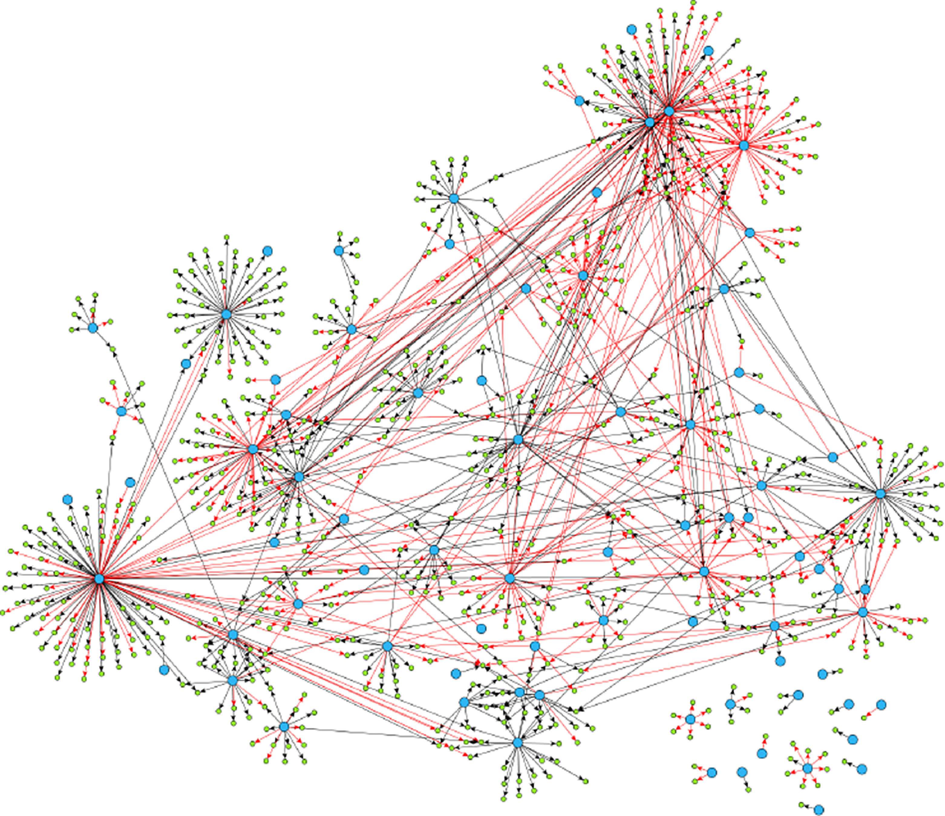
Figure 3. Reproduced under the creative commons attribution license (https://creativecommons.org/licenses/by/4.0/) is a much larger gene regulatory network. It exhibits similar qualitative structure (a network of hub nodes) as does the much smaller network of Figure 2.
For later use, and to get a feel for the topological implications of strong causality, we explore a number of properties of such graphs before moving into the main result of this section. The following important property essentially strengthens Proposition 2.4 for the case of strongly causal graphs.
Proposition 2.5.
In a strongly causal graph, if $j \in{\mathcal{A}({i})}$
then any
$j \in{\mathcal{A}({i})}$
then any $k \in{\mathcal{A}({i})} \cap{\mathcal{A}({j})}$
is not a confounder, that is, the unique path from
$k \in{\mathcal{A}({i})} \cap{\mathcal{A}({j})}$
is not a confounder, that is, the unique path from $k$
to
$k$
to $i$
contains
$i$
contains $j$
.
$j$
.
Proof.
Suppose that there is a path from $k$
to
$k$
to $i$
which does not contain
$i$
which does not contain $j$
. In this case, there are multiple paths from
$j$
. In this case, there are multiple paths from $k$
to
$k$
to $i$
(one of which does go through
$i$
(one of which does go through $j$
, since
$j$
, since $j \in{\mathcal{A}({i})}$
) which contradicts the assumption of strong causality.
$j \in{\mathcal{A}({i})}$
) which contradicts the assumption of strong causality.
Corollary 2.2.
If $\mathcal{G}$
is a strongly causal DAG then
$\mathcal{G}$
is a strongly causal DAG then $i \overset{\text{PW}}{\rightarrow } j$
and
$i \overset{\text{PW}}{\rightarrow } j$
and $j \in{\mathcal{A}({i})}$
are alternatives, that is
$j \in{\mathcal{A}({i})}$
are alternatives, that is $i \overset{\text{PW}}{\rightarrow } j \Rightarrow j \notin{\mathcal{A}({i})}$
.
$i \overset{\text{PW}}{\rightarrow } j \Rightarrow j \notin{\mathcal{A}({i})}$
.
Proof.
Suppose that $i \overset{\text{PW}}{\rightarrow } j$
and
$i \overset{\text{PW}}{\rightarrow } j$
and $j \in{\mathcal{A}({i})}$
. Then since
$j \in{\mathcal{A}({i})}$
. Then since $\mathcal{G}$
is acyclic
$\mathcal{G}$
is acyclic $i \not \in{\mathcal{A}({j})}$
, and by Proposition 2.4 there is some
$i \not \in{\mathcal{A}({j})}$
, and by Proposition 2.4 there is some $k \in{\mathcal{A}({i})}\cap{\mathcal{A}({j})}$
which is a confounder. However, by Proposition 2.5
$k \in{\mathcal{A}({i})}\cap{\mathcal{A}({j})}$
which is a confounder. However, by Proposition 2.5 $k$
cannot be a confounder, a contradiction.
$k$
cannot be a confounder, a contradiction.
Corollary 2.3.
If $\mathcal{G}$
is a strongly causal DAG such that
$\mathcal{G}$
is a strongly causal DAG such that $i \overset{\text{PW}}{\rightarrow } j$
and
$i \overset{\text{PW}}{\rightarrow } j$
and $j \overset{\text{PW}}{\rightarrow } i$
, then
$j \overset{\text{PW}}{\rightarrow } i$
, then $i \not \in{\mathcal{A}({j})}$
and
$i \not \in{\mathcal{A}({j})}$
and $j \not \in{\mathcal{A}({i})}$
. In particular, a pairwise bidirectional edge indicates the absence of any edge in
$j \not \in{\mathcal{A}({i})}$
. In particular, a pairwise bidirectional edge indicates the absence of any edge in $\mathcal{G}$
.
$\mathcal{G}$
.
Proof.
This follows directly from applying Corollary 2.2 to $i \overset{\text{PW}}{\rightarrow } j$
and
$i \overset{\text{PW}}{\rightarrow } j$
and $j \overset{\text{PW}}{\rightarrow } i$
.
$j \overset{\text{PW}}{\rightarrow } i$
.
In light of Proposition 2.5, the following provides a partial converse to Proposition 2.4, and supports the intuition of “causal flow” through paths in $\mathcal{G}$
.
$\mathcal{G}$
.
Proposition 2.6 (Pairwise Causal Flow). If $\mathcal{G}$
is a strongly causal DAG, then
$\mathcal{G}$
is a strongly causal DAG, then $j \in{\mathcal{A}({i})} \Rightarrow j \overset{\text{PW}}{\rightarrow } i$
.
$j \in{\mathcal{A}({i})} \Rightarrow j \overset{\text{PW}}{\rightarrow } i$
.
Proof.
We will show that for some $\psi \in \mathcal{H}_{n-1}^{(j)}$
we have
$\psi \in \mathcal{H}_{n-1}^{(j)}$
we have
 \begin{equation} \langle{\psi -{\hat{\mathbb{E}}[{\psi }\ |\ {\mathcal{H}_{n - 1}^{(i)}}]}},{x_i(n) -{\hat{\mathbb{E}}[x_i(n)\ |\ {\mathcal{H}_{n - 1}^{(i)}}]}}\rangle \ne 0 \end{equation}
and therefore that $H_n^{(i)} \not \perp \ \mathcal{H}_{n-1}^{(j)}\ |\ \mathcal{H}_{n-1}^{(i)}$
, which by Theorem (2.1) is enough to establish that
$H_n^{(i)} \not \perp \ \mathcal{H}_{n-1}^{(j)}\ |\ \mathcal{H}_{n-1}^{(i)}$
, which by Theorem (2.1) is enough to establish that $j \overset{\text{PW}}{\rightarrow } i$
.
$j \overset{\text{PW}}{\rightarrow } i$
.
Firstly, we will establish a representation of $x_i(n)$
that involves
$x_i(n)$
that involves $x_j(n)$
. Denote by
$x_j(n)$
. Denote by $a_{r + 1} \rightarrow a_r \rightarrow \cdots \rightarrow a_1 \rightarrow a_0$
with
$a_{r + 1} \rightarrow a_r \rightarrow \cdots \rightarrow a_1 \rightarrow a_0$
with $a_{r + 1} \;:\!=\; j$
and
$a_{r + 1} \;:\!=\; j$
and $a_0 \;:\!=\; i$
the unique
$a_0 \;:\!=\; i$
the unique $j \rightarrow \cdots \rightarrow i$
path in
$j \rightarrow \cdots \rightarrow i$
path in $\mathcal{G}$
, we will expand the representation of Equation (7) backwards along this path:
$\mathcal{G}$
, we will expand the representation of Equation (7) backwards along this path:
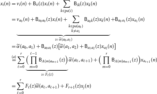 \begin{align*} x_i(n) &= v_i(n) + \mathsf{B}_{ii}(z)x_i(n) + \sum _{k \in{pa(i)}}\mathsf{B}_{ik}(z) x_k(n)\\ &= \underbrace{v_{a_0}(n) + \mathsf{B}_{a_0a_0}(z)x_i(n) + \sum _{\substack{k \in{pa({a_0})} \\ k \ne a_1}}\mathsf{B}_{a_0 k}(z) x_k(n)}_{\;:\!=\;{\widetilde{\alpha }({a_0},{a_1})}} + \mathsf{B}_{a_0a_1}(z)x_{a_1}(n)\\ &={\widetilde{\alpha }({a_0},{a_1})} + \mathsf{B}_{a_0a_1}(z)\big [{\widetilde{\alpha }({a_1},{a_2})} + \mathsf{B}_{a_1a_2}(z)x_{a_2}(n) \big ]\\ &\overset{(a)}{=} \sum _{\ell = 0}^r \underbrace{\Big (\prod _{m = 0}^{\ell - 1} \mathsf{B}_{A(m) a_{m + 1}}(z) \Big )}_{\;:\!=\; F_\ell (z)}{\widetilde{\alpha }({a_\ell },{a_{\ell + 1}})} + \Big (\prod _{m = 0}^{r}\mathsf{B}_{A(m) a_{m + 1}}(z)\Big )x_{a_{r + 1}}(n)\\ &= \sum _{\ell = 0}^r F_\ell (z){\widetilde{\alpha }({a_\ell },{a_{\ell + 1}})} + F_{r + 1}(z) x_j(n) \end{align*}
where $(a)$
follows by a routine induction argument and where we define
$(a)$
follows by a routine induction argument and where we define $\prod _{m = 0}^{-1} \bullet \;:\!=\; 1$
for notational convenience.
$\prod _{m = 0}^{-1} \bullet \;:\!=\; 1$
for notational convenience.
Using this representation to expand Equation (11), we obtain the following cumbersome expression:
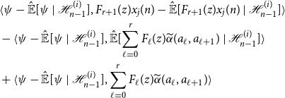 \begin{align*} &\langle{\psi -{\hat{\mathbb{E}}[{\psi }\ |\ {\mathcal{H}_{n - 1}^{(i)}}]}},{F_{r + 1}(z)x_j(n) -{\hat{\mathbb{E}}[{F_{r + 1}(z)x_j(n)}\ |\ {\mathcal{H}_{n - 1}^{(i)}}]}}\rangle \\ &- \langle{\psi -{\hat{\mathbb{E}}[{\psi }\ |\ {\mathcal{H}_{n - 1}^{(i)}}]}},{{\hat{\mathbb{E}}[{\sum _{\ell = 0}^r F_\ell (z){\widetilde{\alpha }({a_\ell },{a_{\ell + 1}})}}\ |\ {\mathcal{H}_{n - 1}^{(i)}}]}}\rangle \\ &+ \langle{\psi -{\hat{\mathbb{E}}[{\psi }\ |\ {\mathcal{H}_{n - 1}^{(i)}}]}},{\sum _{\ell = 0}^r F_\ell (z){\widetilde{\alpha }({a_\ell },{a_{\ell + 1}})}}\rangle \end{align*}
Note that by the orthogonality principle, $\psi -{\hat{\mathbb{E}}[{\psi }\ |\ {\mathcal{H}_{n - 1}^{(i)}}]} \perp \mathcal{H}_{n-1}^{(i)}$
, the middle term above is
$\psi -{\hat{\mathbb{E}}[{\psi }\ |\ {\mathcal{H}_{n - 1}^{(i)}}]} \perp \mathcal{H}_{n-1}^{(i)}$
, the middle term above is $0$
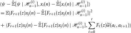
. Choosing now the particular value
$0$
. Choosing now the particular value $\psi = F_{r + 1}(z)x_j(n) \in \mathcal{H}_{n-1}^{(j)}$
we arrive at
$\psi = F_{r + 1}(z)x_j(n) \in \mathcal{H}_{n-1}^{(j)}$
we arrive at
 \begin{align*} &\langle{\psi -{\hat{\mathbb{E}}[{\psi }\ |\ {\mathcal{H}_{n - 1}^{(i)}}]}},{x_i(n) -{\hat{\mathbb{E}}[{x_i(n)}\ |\ {\mathcal{H}_{n - 1}^{(i)}}]}}\rangle \\ &= \mathbb{E}|F_{r + 1}(z)x_j(n) -{\hat{\mathbb{E}}[{F_{r + 1}(z)x_j(n)}\ |\ {\mathcal{H}_{n - 1}^{(i)}}]}|^2\\ &+ \langle{F_{r + 1}(z)x_j(n) -{\hat{\mathbb{E}}[{F_{r + 1}(z)x_j(n)}\ |\ {\mathcal{H}_{n - 1}^{(i)}}]}},{\sum _{\ell = 0}^r F_\ell (z){\widetilde{\alpha }({a_\ell },{a_{\ell + 1}})}}\rangle \end{align*}
Now since $F_{r + 1}(z) \ne 0$
by Theorem 2.1, and
$F_{r + 1}(z) \ne 0$
by Theorem 2.1, and $F_{r + 1}(z)x_j(n) \not \in \mathcal{H}_{n-1}^{(i)}$
, we have by the Cauchy-Schwarz inequality that this expression is equal to
$F_{r + 1}(z)x_j(n) \not \in \mathcal{H}_{n-1}^{(i)}$
, we have by the Cauchy-Schwarz inequality that this expression is equal to $0$
if and only if
$0$
if and only if
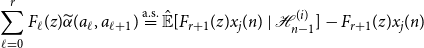 \begin{equation*} \sum _{\ell = 0}^r F_\ell (z) {\widetilde {\alpha }({a_\ell }, {a_{\ell + 1}})} \overset {\text {a.s.}}{=} {\hat {\mathbb {E}}[{F_{r + 1}(z)x_j(n)}\ |\ {\mathcal {H}_{n - 1}^{(i)}}]} - F_{r + 1}(z)x_j(n) \end{equation*}
or by rearranging and applying the representation for $x_i(n)$
obtained earlier, if and only if
$x_i(n)$
obtained earlier, if and only if
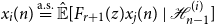 \begin{equation*} x_i(n) \overset {\text {a.s.}}{=} {\hat {\mathbb {E}}[{F_{r + 1}(z)x_j(n)}\ |\ {\mathcal {H}_{n - 1}^{(i)}}]} \end{equation*}
But, this is impossible since $x_i(n) \not \in\mathcal{H}_{n - 1}^{(i)}$
.
$x_i(n) \not \in\mathcal{H}_{n - 1}^{(i)}$
.
We immediately obtain the corollary, which we remind the reader is, surprisingly, not true in a general graph.
Corollary 2.4.
If $\mathcal{G}$
is a strongly causal DAG then
$\mathcal{G}$
is a strongly causal DAG then $j \overset{\text{GC}}{\rightarrow } i \Rightarrow j \overset{\text{PW}}{\rightarrow } i$
.
$j \overset{\text{GC}}{\rightarrow } i \Rightarrow j \overset{\text{PW}}{\rightarrow } i$
.
Example 2.2. As a final remark of this subsection we note that a complete converse to Proposition 2.4 is not possible without additional conditions. Consider the “fork” system on $3$
nodes (i.e.,
$3$
nodes (i.e., $2 \leftarrow 1 \rightarrow 3$
) defined by
$2 \leftarrow 1 \rightarrow 3$
) defined by
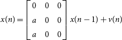 \begin{equation*} x(n) = \left [ \begin {array}{c@{\quad}c@{\quad}c} 0 & 0 & 0\\ a & 0 & 0\\ a & 0 & 0\\ \end {array} \right ] x(n - 1) + v(n) \end{equation*}
In this case, node $1$
is a confounder for nodes
$1$
is a confounder for nodes $2$
and
$2$
and $3$
, but
$3$
, but $x_3(n) = v_3(n) - v_2(n) + x_2(n)$
and
$x_3(n) = v_3(n) - v_2(n) + x_2(n)$
and $2 \overset{\text{PW}}{\nrightarrow } 3$
(even though
$2 \overset{\text{PW}}{\nrightarrow } 3$
(even though $x_2(n)$
and
$x_2(n)$
and $x_3(n)$
are contemporaneously correlated).
$x_3(n)$
are contemporaneously correlated).
If we were to augment this system by simply adding an autoregressive component (i.e., some “memory”) to $x_1(n)$
, for example,
$x_1(n)$
, for example, $x_1(n) = v_1(n) + b x_1(n - 1)$
then we would have
$x_1(n) = v_1(n) + b x_1(n - 1)$
then we would have $2 \overset{\text{PW}}{\rightarrow } 3$
since then
$2 \overset{\text{PW}}{\rightarrow } 3$
since then $x_3(n) = v_3(n) + av_1(n - 1) - bv_2(n - 1) + bx_2(n - 1)$
. We develop this idea further in the next section.
$x_3(n) = v_3(n) + av_1(n - 1) - bv_2(n - 1) + bx_2(n - 1)$
. We develop this idea further in the next section.
2.6 Persistent systems
In Section 2.5 we obtained a converse to part $(a)$
of Proposition 2.4 via the notion of a strongly causal graph topology (see Proposition 2.6). In this section, we study conditions under which a converse to part
$(a)$
of Proposition 2.4 via the notion of a strongly causal graph topology (see Proposition 2.6). In this section, we study conditions under which a converse to part $(b)$
will hold.
$(b)$
will hold.
Definition 2.10 (Lag Function). Given a causal filter $\mathsf{B}(z) = \sum _{m = 0}^\infty b(m)z^{-m}$
define
$\mathsf{B}(z) = \sum _{m = 0}^\infty b(m)z^{-m}$
define
 \begin{align} m_0(\mathsf{B}) &= \text{inf }\{m \in \mathbb{Z}_+\ |\ b(m) \ne 0\} \end{align}
 \begin{align} m_{\infty }(\mathsf{B}) &= \text{sup }\{m \in \mathbb{Z}_+\ |\ b(m) \ne 0\} \end{align}
that is, the “first” and “last” coefficients of the filter $\mathsf{B}(z)$
, where
$\mathsf{B}(z)$
, where $m_\infty (\mathsf{B}) \;:\!=\; \infty$
if the filter has an infinite length, and
$m_\infty (\mathsf{B}) \;:\!=\; \infty$
if the filter has an infinite length, and $m_0(\mathsf{B}) \;:\!=\; \infty$
if
$m_0(\mathsf{B}) \;:\!=\; \infty$
if $\mathsf{B}(z) = 0$
.
$\mathsf{B}(z) = 0$
.
Definition 2.11 (Persistent). We will say that the process $x(n)$
with Granger causality graph
$x(n)$
with Granger causality graph $\mathcal{G}$
is persistent if for every
$\mathcal{G}$
is persistent if for every $i \in [N]$
and every
$i \in [N]$
and every $k \in{\mathcal{A}({i})}$
we have
$k \in{\mathcal{A}({i})}$
we have $m_0(\mathsf{A}_{ik}) \lt \infty$
and
$m_0(\mathsf{A}_{ik}) \lt \infty$
and $m_\infty (\mathsf{A}_{ik}) = \infty$
.
$m_\infty (\mathsf{A}_{ik}) = \infty$
.
Remark 2.3. In the context of Granger causality, “most” systems should be persistent. In particular, $\mathsf{\mathsf{VAR}}(p)$
models are likely to be persistent since these naturally result in an equivalent
$\mathsf{\mathsf{VAR}}(p)$
models are likely to be persistent since these naturally result in an equivalent $\mathsf{MA}(\infty )$
representation, see Example 2.3 for a more formal statement.
$\mathsf{MA}(\infty )$
representation, see Example 2.3 for a more formal statement.
Moreover, persistence is not the weakest condition necessary for the results of this section: by inspecting our proofs, the condition that for each $i, j$
there is some
$i, j$
there is some $k \in{\mathcal{A}({i})}\cap{\mathcal{A}({j})}$
such that
$k \in{\mathcal{A}({i})}\cap{\mathcal{A}({j})}$
such that $m_0(\mathsf{A}_{jk}) \lt m_\infty (\mathsf{A}_{ik})$
can be seen to be sufficient. The intuition being that nodes
$m_0(\mathsf{A}_{jk}) \lt m_\infty (\mathsf{A}_{ik})$
can be seen to be sufficient. The intuition being that nodes $i$
and
$i$
and $j$
are not receiving temporally disjoint information from
$j$
are not receiving temporally disjoint information from $k$
.
$k$
.
The etymology for the persistence condition can be explained by supposing that the two nodes $i, j$
each have a loop (i.e.,
$i, j$
each have a loop (i.e., $\mathsf{B}_{ii}(z) \ne 0, \mathsf{B}_{jj}(z) \ne 0$
) then this autoregressive component acts as “memory,” and so the influence from the confounder
$\mathsf{B}_{ii}(z) \ne 0, \mathsf{B}_{jj}(z) \ne 0$
) then this autoregressive component acts as “memory,” and so the influence from the confounder $k$
persists in
$k$
persists in $x_i(n)$
, and
$x_i(n)$
, and $m_\infty (\mathsf{A}_{ik}) = \infty$
for each confounder can be expected.
$m_\infty (\mathsf{A}_{ik}) = \infty$
for each confounder can be expected.
Example 2.3 (Ubiquity of Persistent Systems; Proof in Section D.2). Consider a process $x(n)$
generated by the
$x(n)$
generated by the $\mathsf{VAR}(1)$
modelFootnote 2 having
$\mathsf{VAR}(1)$
modelFootnote 2 having $\mathsf{B}(z) = Bz^{-1}$
. If
$\mathsf{B}(z) = Bz^{-1}$
. If $B$
is diagonalizable, and has at least
$B$
is diagonalizable, and has at least $2$
distinct eigenvalues, then
$2$
distinct eigenvalues, then $x(n)$
is persistent. A proof of this fact is provided in the Appendix.
$x(n)$
is persistent. A proof of this fact is provided in the Appendix.
This example shows that the collection of finite $\mathsf{VAR}(p)$
systems which are not persistent are pathological, in the sense that their system matrices have zero measure.
$\mathsf{VAR}(p)$
systems which are not persistent are pathological, in the sense that their system matrices have zero measure.
In order to eliminate the possibility of a particular sort of cancelation, an ad hoc assumption is required. Strictly speaking, the persistence condition is not a necessary or sufficient condition for the following, but cases where the following fails to hold, and persistence does hold, are unavoidable pathologies.
Assumption 2.1 (no-cancellation). Fix $i, j \in [N]$
and let
$i, j \in [N]$
and let $H_i(z)$
be the strictly causal filter such that
$H_i(z)$
be the strictly causal filter such that
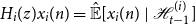 \begin{equation*} H_i(z)x_i(n) = {\hat {\mathbb {E}}[{x_i(n)}\ |\ {\mathcal {H}_{t - 1}^{(i)}}]} \end{equation*}
and similarly for $H_j(z)$
. Then define
$H_j(z)$
. Then define
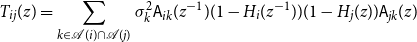 \begin{equation} T_{ij}(z)= \sum _{k \in{\mathcal{A}({i})} \cap{\mathcal{A}({j})}}\sigma _k^2\mathsf{A}_{ik}(z^{-1}) (1 - H_i(z^{-1})) (1 - H_j(z))\mathsf{A}_{jk}(z) \end{equation}
where $\sigma _k^2 = \mathbb{E} v_k(n)^2$
.
$\sigma _k^2 = \mathbb{E} v_k(n)^2$
.
We will say that Assumption
2.1
is satisfied if for every $i, j \in [N]$
,
$i, j \in [N]$
, $T_{ij}(z)$
is either constant over
$T_{ij}(z)$
is either constant over $z$
(i.e., each
$z$
(i.e., each $z^k$
coefficient for
$z^k$
coefficient for $k \in \mathbb{Z} \setminus \{0\}$
is
$k \in \mathbb{Z} \setminus \{0\}$
is $0$
), or is neither causal (i.e., containing only
$0$
), or is neither causal (i.e., containing only $z^{-k}$
terms, for
$z^{-k}$
terms, for $k \ge 0$
) or anti-causal (i.e., containing only
$k \ge 0$
) or anti-causal (i.e., containing only $z^k$
terms, for
$z^k$
terms, for $k \ge 0$
). Put succinctly,
$k \ge 0$
). Put succinctly, $T_{ij}(z)$
must be two-sided.
$T_{ij}(z)$
must be two-sided.
Remark 2.4. Under the condition of persistence, the only way for Assumption 2.1 to fail is through cancelation in the terms defining $T_{ij}(z)$
. For example, the condition is assured if
$T_{ij}(z)$
. For example, the condition is assured if $x(n)$
is persistent, and there is only a single confounder. Unfortunately, some pathological behavior resulting from confounding nodes seems to be unavoidable without some assumptions (regarding sets of zero measure) about the parameters of the
$x(n)$
is persistent, and there is only a single confounder. Unfortunately, some pathological behavior resulting from confounding nodes seems to be unavoidable without some assumptions (regarding sets of zero measure) about the parameters of the $\mathsf{MA}(\infty )$
system defining
$\mathsf{MA}(\infty )$
system defining $x(n)$
.
$x(n)$
.
Proposition 2.7 (Pairwise Causation and Confounders). Fix $i, j \in [N]$
and suppose
$i, j \in [N]$
and suppose $\exists k \in{\mathcal{A}({i})} \cap{\mathcal{A}({j})}$
which confounds
$\exists k \in{\mathcal{A}({i})} \cap{\mathcal{A}({j})}$
which confounds $i, j$
. Then, if
$i, j$
. Then, if $T_{ij}(z)$
is not causal we have
$T_{ij}(z)$
is not causal we have $j \overset{\text{PW}}{\rightarrow } i$
, and if
$j \overset{\text{PW}}{\rightarrow } i$
, and if $T_{ij}(z)$
is not anti-causal we have
$T_{ij}(z)$
is not anti-causal we have $i \overset{\text{PW}}{\rightarrow } j$
. Moreover, if Assumption
2.1
is satisfied, then
$i \overset{\text{PW}}{\rightarrow } j$
. Moreover, if Assumption
2.1
is satisfied, then $j \overset{\text{PW}}{\rightarrow } i \iff i \overset{\text{PW}}{\rightarrow } j$
.
$j \overset{\text{PW}}{\rightarrow } i \iff i \overset{\text{PW}}{\rightarrow } j$
.
Proof.
Recalling Theorem 2.1, consider some $\psi \in \mathcal{H}_{n-1}^{(j)}$
and represent it as
$\psi \in \mathcal{H}_{n-1}^{(j)}$
and represent it as $\psi (n) = F(z)x_j(n)$
for some strictly causal filter
$\psi (n) = F(z)x_j(n)$
for some strictly causal filter $F(z)$
. Then
$F(z)$
. Then
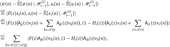 \begin{align*} &\langle{\psi (n) -{\hat{\mathbb{E}}[{\psi (n)}\ |\ {\mathcal{H}_{t - 1}^{(i)}}]}},{x_i(n) -{\hat{\mathbb{E}}[{x_i(n)}\ |\ {\mathcal{H}_{t - 1}^{(i)}}]}}\rangle \\ &\overset{(a)}{=} \langle{F(z)x_j(n)},{x_i(n) -{\hat{\mathbb{E}}[{x_i(n)}\ |\ {\mathcal{H}_{t - 1}^{(i)}}]}}\rangle \\ &\overset{(b)}{=} \langle{F(z)\big (\mathsf{A}_{jj}(z)v_j(n) + \sum _{k \in{\mathcal{A}({j})}}\mathsf{A}_{jk}(z)v_k(n)\big )},{(1 - H_i(z))\big (\mathsf{A}_{ii}(z)v_i(n) + \sum _{\ell \in{\mathcal{A}({i})}}\mathsf{A}_{i\ell }(z)v_\ell (n)\big )}\rangle \\ &\overset{(c)}{=} \sum _{k \in{\mathcal{A}({i})}\cap{\mathcal{A}({j})}}\langle{F(z)\mathsf{A}_{jk}(z)v_k(n)},{(1 - H_i(z))\mathsf{A}_{ik}(z)v_k(n)}\rangle, \end{align*}
where $(a)$
applies the orthogonality principle,
$(a)$
applies the orthogonality principle, $(b)$
expands with Equation (8) with
$(b)$
expands with Equation (8) with $H_i(z)x_i(n) ={\hat{\mathbb{E}}[{x_i(n)}\ |\ {\mathcal{H}_{t - 1}^{(i)}}]}$
, and
$H_i(z)x_i(n) ={\hat{\mathbb{E}}[{x_i(n)}\ |\ {\mathcal{H}_{t - 1}^{(i)}}]}$
, and $(c)$
follows by performing cancelations of
$(c)$
follows by performing cancelations of $v_k(n) \perp v_\ell (n)$
and noting that by the contra-positive of Proposition 2.5 we cannot have
$v_k(n) \perp v_\ell (n)$
and noting that by the contra-positive of Proposition 2.5 we cannot have $i \in{\mathcal{A}({j})}$
or
$i \in{\mathcal{A}({j})}$
or $j \in{\mathcal{A}({i})}$
.
$j \in{\mathcal{A}({i})}$
.
Through symmetric calculation, we can obtain the expression relevant to the determination of $i \overset{\text{PW}}{\rightarrow } j$
for
$i \overset{\text{PW}}{\rightarrow } j$
for $\phi \in \mathcal{H}_{n-1}^{(i)}$
represented by the strictly causal filter
$\phi \in \mathcal{H}_{n-1}^{(i)}$
represented by the strictly causal filter $G(z)\;:\; \phi (n) = G(z)x_i(n)$
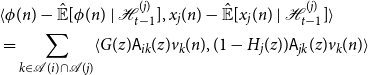 \begin{align*} &\langle{\phi (n) -{\hat{\mathbb{E}}[{\phi (n)}\ |\ {\mathcal{H}_{t - 1}^{(j)}}]}},{x_j(n) -{\hat{\mathbb{E}}[{x_j(n)}\ |\ {\mathcal{H}_{t - 1}^{(j)}}]}}\rangle \\ &= \sum _{k \in{\mathcal{A}({i})} \cap{\mathcal{A}({j})}}\langle{G(z)\mathsf{A}_{ik}(z)v_k(n)},{(1 - H_j(z))\mathsf{A}_{jk}(z)v_k(n)}\rangle \end{align*}
where $H_j(z)x_j(n) ={\hat{\mathbb{E}}[{x_j(n)}\ |\ {\mathcal{H}_{t - 1}^{(j)}}]}$
.
$H_j(z)x_j(n) ={\hat{\mathbb{E}}[{x_j(n)}\ |\ {\mathcal{H}_{t - 1}^{(j)}}]}$
.
We have therefore
 \begin{align} (j \overset{\text{PW}}{\rightarrow } i)\;:\; \exists F(z) \text{ s.t. } \sum _{k \in{\mathcal{A}({i})} \cap{\mathcal{A}({j})}}\langle{F(z)\mathsf{A}_{jk}(z)v_k(n)},{(1 - H_i(z))\mathsf{A}_{ik}(z)v_k(n)}\rangle \ne 0 \end{align}
 \begin{align} (i \overset{\text{PW}}{\rightarrow } j)\;:\; \exists G(z) \text{ s.t. } \sum _{k \in{\mathcal{A}({i})} \cap{\mathcal{A}({j})}}\langle{G(z)\mathsf{A}_{ik}(z)v_k(n)},{(1 - H_j(z))\mathsf{A}_{jk}(z)v_k(n)}\rangle \ne 0 \end{align}
The persistence condition, by Corollary D.1, ensures that for each $k \in{\mathcal{A}({i})}\cap{\mathcal{A}({j})}$
there is some
$k \in{\mathcal{A}({i})}\cap{\mathcal{A}({j})}$
there is some $F(z)$
and some
$F(z)$
and some $G(z)$
such that at least one of the above terms constituting the sum over
$G(z)$
such that at least one of the above terms constituting the sum over $k$
is non-zero. It remains to eliminate the possibility of cancelation in the sum.
$k$
is non-zero. It remains to eliminate the possibility of cancelation in the sum.
The adjoint of a linear filter $C(z)$
is simply
$C(z)$
is simply $C(z^{-1})$
, which recall is strictly anti-causal if
$C(z^{-1})$
, which recall is strictly anti-causal if $C(z)$
is strictly causal. Using this, we can write
$C(z)$
is strictly causal. Using this, we can write
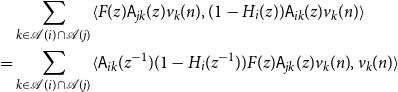 \begin{align*} &\sum _{k \in{\mathcal{A}({i})} \cap{\mathcal{A}({j})}}\langle{F(z)\mathsf{A}_{jk}(z)v_k(n)},{(1 - H_i(z))\mathsf{A}_{ik}(z)v_k(n)}\rangle \\ = &\sum _{k \in{\mathcal{A}({i})} \cap{\mathcal{A}({j})}}\langle{\mathsf{A}_{ik}(z^{-1})(1 - H_i(z^{-1}))F(z)\mathsf{A}_{jk}(z)v_k(n)},{v_k(n)}\rangle \end{align*}
Moreover, it is sufficient to find some strictly causal $F(z)$
of the form
$F(z)$
of the form $F(z)(1 - H_j(z))$
(abusing notation) since
$F(z)(1 - H_j(z))$
(abusing notation) since $1 - H_j(z)$
is causal. Similarly for
$1 - H_j(z)$
is causal. Similarly for $G(z)$
, this leads to symmetric expressions for
$G(z)$
, this leads to symmetric expressions for $j \overset{\text{PW}}{\rightarrow } i$
and
$j \overset{\text{PW}}{\rightarrow } i$
and $i \overset{\text{PW}}{\rightarrow } j$
respectively:
$i \overset{\text{PW}}{\rightarrow } j$
respectively:
 \begin{equation} \sum _{k \in{\mathcal{A}({i})} \cap{\mathcal{A}({j})}}\langle{\mathsf{A}_{ik}(z^{-1})(1 - H_i(z^{-1}))F(z)(1 - H_j(z))\mathsf{A}_{jk}(z)v_k(n)},{v_k(n)}\rangle \end{equation}
 \begin{equation} \sum _{k \in{\mathcal{A}({i})} \cap{\mathcal{A}({j})}}\langle{\mathsf{A}_{ik}(z^{-1})(1 - H_i(z^{-1}))G(z^{-1})(1 - H_j(z))\mathsf{A}_{jk}(z)v_k(n)},{v_k(n)}\rangle \end{equation}
Recall the filter from Assumption 2.1
 \begin{equation} T_{ij}(z) = \sum _{k \in{\mathcal{A}({i})} \cap{\mathcal{A}({j})}} \sigma _k^2\mathsf{A}_{ik}(z^{-1})(1 - H_i(z^{-1}))(1 - H_j(z))\mathsf{A}_{jk}(z) \end{equation}
Since each $v_k(n)$
is uncorrelated through time,
$v_k(n)$
is uncorrelated through time, $\langle{T_{ij}(z)v_k(n)},{v_k(n)}\rangle = \sigma _k^2T_{ij}(0)$
, and therefore we have
$\langle{T_{ij}(z)v_k(n)},{v_k(n)}\rangle = \sigma _k^2T_{ij}(0)$
, and therefore we have $j \overset{\text{PW}}{\rightarrow } i$
if
$j \overset{\text{PW}}{\rightarrow } i$
if $T_{ij}(z)$
is not causal and
$T_{ij}(z)$
is not causal and $i \overset{\text{PW}}{\rightarrow } j$
if
$i \overset{\text{PW}}{\rightarrow } j$
if $T_{ij}(z)$
it not anti-causal. Moreover, we have
$T_{ij}(z)$
it not anti-causal. Moreover, we have $i \overset{\text{PW}}{\nrightarrow } j$
and
$i \overset{\text{PW}}{\nrightarrow } j$
and $j \overset{\text{PW}}{\rightarrow } i$
if
$j \overset{\text{PW}}{\rightarrow } i$
if $T_{ij}(z)$
is a constant. Therefore, under Assumption 2.1
$T_{ij}(z)$
is a constant. Therefore, under Assumption 2.1 $j \overset{\text{PW}}{\rightarrow } i \iff i \overset{\text{PW}}{\rightarrow } j$
.
$j \overset{\text{PW}}{\rightarrow } i \iff i \overset{\text{PW}}{\rightarrow } j$
.
This follows since if $T_{ij}(z)$
is not causal then
$T_{ij}(z)$
is not causal then $\exists k \gt 0$
such that the
$\exists k \gt 0$
such that the $z^k$
coefficient of
$z^k$
coefficient of $T_{ij}(z)$
is non-zero, and we can choose strictly causal
$T_{ij}(z)$
is non-zero, and we can choose strictly causal $F(z) = z^{-k}$
such that (D11) is non-zero and therefore
$F(z) = z^{-k}$
such that (D11) is non-zero and therefore $j \overset{\text{PW}}{\rightarrow } i$
.
$j \overset{\text{PW}}{\rightarrow } i$
.
Similarly, if $T_{ij}(z)$
is not anti-causal, then
$T_{ij}(z)$
is not anti-causal, then $\exists k \gt 0$
such that the
$\exists k \gt 0$
such that the $z^{-k}$
coefficient of
$z^{-k}$
coefficient of $T_{ij}(z)$
is non-zero, and we can choose strictly causal
$T_{ij}(z)$
is non-zero, and we can choose strictly causal $G(z)$
so that
$G(z)$
so that $G(z^{-1}) = z^k$
, and then (D12) is non-zero and therefore
$G(z^{-1}) = z^k$
, and then (D12) is non-zero and therefore $i \overset{\text{PW}}{\rightarrow } j$
.
$i \overset{\text{PW}}{\rightarrow } j$
.
Remark 2.5. The importance of this result is that when $i \overset{\text{PW}}{\rightarrow } j$
is a result of a confounder
$i \overset{\text{PW}}{\rightarrow } j$
is a result of a confounder $k$
, then
$k$
, then $i \overset{\text{PW}}{\rightarrow } j \iff j \overset{\text{PW}}{\rightarrow } i$
. This implies that in a strongly causal graph every bidirectional pairwise causality relation must be the result of a confounder. Therefore, in a strongly causal graph, pairwise causality analysis is immune to confounding (since we can safely remove all bidirectional edges).
$i \overset{\text{PW}}{\rightarrow } j \iff j \overset{\text{PW}}{\rightarrow } i$
. This implies that in a strongly causal graph every bidirectional pairwise causality relation must be the result of a confounder. Therefore, in a strongly causal graph, pairwise causality analysis is immune to confounding (since we can safely remove all bidirectional edges).
2.7 Recovering
$\mathcal{G}$
via pairwise tests

We arrive at the main conclusion of the theoretical analysis in this paper.
Theorem 2.2 (Pairwise Recovery; Proof in Section D.3). If the Granger causality graph $\mathcal{G}$
for the process
$\mathcal{G}$
for the process $x(n)$
is a strongly causal DAG and Assumption
2.1
holds, then
$x(n)$
is a strongly causal DAG and Assumption
2.1
holds, then $\mathcal{G}$
can be inferred from pairwise causality tests. The procedure can be carried out, assuming we have an oracle for pairwise causality, via Algorithm (
1
).
$\mathcal{G}$
can be inferred from pairwise causality tests. The procedure can be carried out, assuming we have an oracle for pairwise causality, via Algorithm (
1
).
Algorithm 1: Pairwise Granger Causality Algorithm
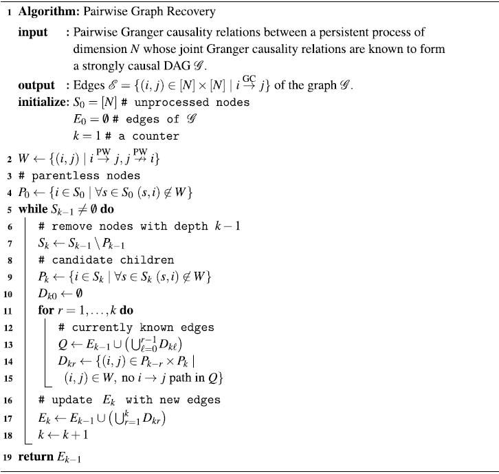
Example 2.4. The set $W$
of Algorithm 1 collects ancestor relations in
$W$
of Algorithm 1 collects ancestor relations in $\mathcal{G}$
(see Lemma D.5). In reference to Figure 4, each of the solid black edges, as well as the dotted red edges will be included in
$\mathcal{G}$
(see Lemma D.5). In reference to Figure 4, each of the solid black edges, as well as the dotted red edges will be included in $W$
, but not the bidirectional green dash-dotted edges, which we are able to exclude as results of confounding. The groupings
$W$
, but not the bidirectional green dash-dotted edges, which we are able to exclude as results of confounding. The groupings $P_0, \ldots, P_3$
are also indicated in Figure 4.
$P_0, \ldots, P_3$
are also indicated in Figure 4.
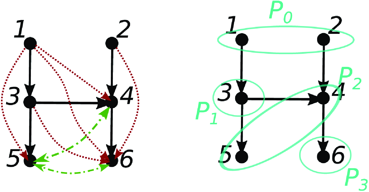
Figure 4. Black arrows indicate true parent-child relations. Red dotted arrows indicate pairwise causality (due to non-parent relations), green dash-dotted arrows indicate bidirectional pairwise causality (due to the confounding node $1$
). Blue groupings indicate each
$1$
). Blue groupings indicate each $P_k$
in Algorithm 1.
$P_k$
in Algorithm 1.
The algorithm proceeds first with the parent-less nodes $1, 2$
on the initial iteration where the edge
$1, 2$
on the initial iteration where the edge $(1, 3)$
is added to
$(1, 3)$
is added to $E$
. On the next iteration, the edges
$E$
. On the next iteration, the edges $(3, 4), (2, 4), (3, 5)$
are added, and the false edges
$(3, 4), (2, 4), (3, 5)$
are added, and the false edges $(1, 4), (1, 5)$
are excluded due to the paths
$(1, 4), (1, 5)$
are excluded due to the paths $1 \rightarrow 3 \rightarrow 4$
and
$1 \rightarrow 3 \rightarrow 4$
and $1 \rightarrow 3 \rightarrow 5$
already being present. Finally, edge
$1 \rightarrow 3 \rightarrow 5$
already being present. Finally, edge $(4, 6)$
is added, and the false
$(4, 6)$
is added, and the false $(1, 6), (3, 6), (2, 6)$
edges are similarly excluded due to the ordering of the inner loop.
$(1, 6), (3, 6), (2, 6)$
edges are similarly excluded due to the ordering of the inner loop.
That we need to proceed backwards through $P_{k - r}$
as in the inner loop on
$P_{k - r}$
as in the inner loop on $r$
can also be seen from this example, where if instead we simply added the set
$r$
can also be seen from this example, where if instead we simply added the set
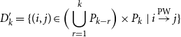 \begin{equation*} D_k' = \{(i, j) \in \Big (\bigcup _{r = 1}^k P_{k - r}\Big ) \times P_k\ |\ i \overset {\text {PW}}{\rightarrow } j \} \end{equation*}
to $E_k$
then we would infer the false positive edge
$E_k$
then we would infer the false positive edge $1 \rightarrow 4$
. Moreover, the same example shows that simply using the set
$1 \rightarrow 4$
. Moreover, the same example shows that simply using the set
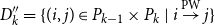 \begin{equation*} D_k'' = \{(i, j) \in P_{k - 1} \times P_k\ |\ i \overset {\text {PW}}{\rightarrow } j \} \end{equation*}
causes the edge $1 \rightarrow 3$
to be missed.
$1 \rightarrow 3$
to be missed.
3. Simulations
We implement an heuristic inspired by Algorithm 1 by replacing the population statistics with finite sample tests, the details of which can be found in the supplementary material Section B.5 (see Algorithm 2). The heuristic is essentially controlling the false discovery rate substantially below what it would be with a threshold based pairwise scheme. The methods are easily parallelizable, and can scale to graphs with thousands of nodes on simple personal computers. By contrast, scaling the LASSO to this large of a network (millions of variables) is not trivial.
We first ran experiments using two separate graph topologies having $N = 50$
nodes, and with a total of
$N = 50$
nodes, and with a total of $T$
samples drawn from the resulting system. The graphs we consider are a strongly causal graph (SCG) and a directed acyclic graph (DAG), and the filters along each edges are constructed by uniformly at random placing
$T$
samples drawn from the resulting system. The graphs we consider are a strongly causal graph (SCG) and a directed acyclic graph (DAG), and the filters along each edges are constructed by uniformly at random placing $p = 5$
poles in a disc of radius
$p = 5$
poles in a disc of radius $3/4$
. We compare our results against the adaptive LASSO (adaLASSO) (Zou, Reference Zou2006), which, since it enjoys the oracle property should be expected to, asymptotically, fully recover the underlying causality graph. Indeed, we found early on that this LASSO variant drastically out-performed alternative LASSO-based procedures including the ordinary LASSO, grouped LASSO, and elastic net by wide margins.
$3/4$
. We compare our results against the adaptive LASSO (adaLASSO) (Zou, Reference Zou2006), which, since it enjoys the oracle property should be expected to, asymptotically, fully recover the underlying causality graph. Indeed, we found early on that this LASSO variant drastically out-performed alternative LASSO-based procedures including the ordinary LASSO, grouped LASSO, and elastic net by wide margins.
The usual methodology of applying the LASSO to Granger causality is to split the square one-step-ahead prediction error into separate terms, one for each group of incident edges on a node, and estimating the collection of $N$
incident filters
$N$
incident filters $\big \{\mathsf{B}_{ij}(z)\big \}_{j = 1}^N$
that minimizes
$\big \{\mathsf{B}_{ij}(z)\big \}_{j = 1}^N$
that minimizes $\xi _i^{\text{LASSO}}$
in the following:
$\xi _i^{\text{LASSO}}$
in the following:
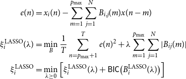 \begin{equation} \begin{aligned} e(n) &=x_i(n) - \sum _{m = 1}^{p_{\text{max}}}\sum _{j = 1}^N B_{i, j}(m) x(n - m)\\ \xi _i^{\text{LASSO}}(\lambda ) &= \underset{B}{\text{min}}\ \frac{1}{T}\sum _{n = p_{\text{max}} + 1}^Te(n)^2 + \lambda \sum _{m = 1}^{p_{\text{max}}} \sum _{j = 1}^N |B_{ij}(m)|\\ \xi _i^{\text{LASSO}} &= \underset{\lambda \ge 0}{\text{min}}\ \Bigl [\xi _i^{\text{LASSO}}(\lambda ) + \mathsf{BIC}\big (B_i^{\text{LASSO}}(\lambda )\big )\Bigr ]\\ \end{aligned} \end{equation}
where we are choosing $\lambda$
, the regularization parameters, via the Bayesian Information Criteria (see, i.e., Claeskens et al. (Reference Claeskens and Hjort2008)). This is similar to the work of Arnold et al. (Reference Arnold, Liu and Abe2007), except that we have replaced the LASSO with the better performing adaLASSO.
$\lambda$
, the regularization parameters, via the Bayesian Information Criteria (see, i.e., Claeskens et al. (Reference Claeskens and Hjort2008)). This is similar to the work of Arnold et al. (Reference Arnold, Liu and Abe2007), except that we have replaced the LASSO with the better performing adaLASSO.
Remark 3.1 (Graph Topologies). We depict in Figure 5 some representative graph topologies used in our empirical evaluation. To construct these graphs we first use simple Erdos-Renyi graphs $\mathcal{G}(N, q)$
with
$\mathcal{G}(N, q)$
with $N$
nodes and edge probability
$N$
nodes and edge probability $q$
, and then remove edges until the graph is acyclic. For values of
$q$
, and then remove edges until the graph is acyclic. For values of $q$
close to
$q$
close to $\frac{2}{n}$
, the resulting random graphs tend to have a topology which is, at least qualitatively, close to the SCG. As the value of
$\frac{2}{n}$
, the resulting random graphs tend to have a topology which is, at least qualitatively, close to the SCG. As the value of $q$
increases, the random graphs deviate farther from the SCG topology, and we therefore expect the LASSO to outperform PWGC for larger values of
$q$
increases, the random graphs deviate farther from the SCG topology, and we therefore expect the LASSO to outperform PWGC for larger values of $q$
.
$q$
.
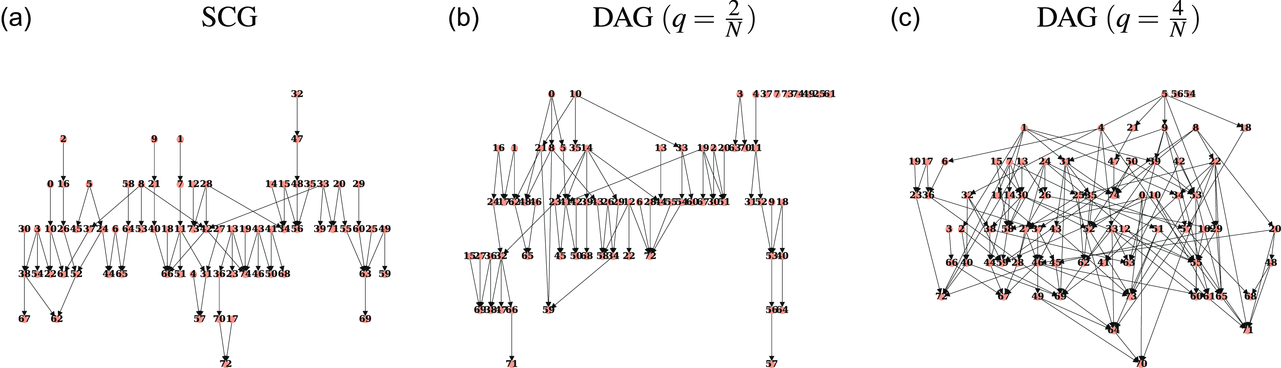
Figure 5. Representative random graph topologies on $N = 50$
nodes.
$N = 50$
nodes.
Remark 3.2 (MCC as a Support Recovery Measurement). We apply Matthew’s Correlation Coefficient (MCC) (Matthews, Reference Matthews1975; Chicco & Jurman, Reference Chicco and Jurman2020) as a statistic for measuring support recovery performance (see also Chicco (Reference Chicco2017) tip # 8). This statistic synthesizes the confusion matrix into a single score appropriate for unbalanced labels and is calibrated to fall into the range $[-1, 1]$
with
$[-1, 1]$
with $1$
being perfect performance,
$1$
being perfect performance, $0$
being the performance of random selection, and
$0$
being the performance of random selection, and $-1$
being perfectly opposed.
$-1$
being perfectly opposed.
Remark 3.3 (Error Measurement). We estimate the out of sample 1-step ahead prediction error by forming the variance matrix estimate
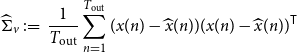 \begin{equation*} \widehat {\Sigma }_v \;:\!=\; \frac {1}{T_{\text {out}}} \sum _{n = 1}^{T_{\text {out}}} (x(n) - \widehat {x}(n))(x(n) - \widehat {x}(n))^{\mathsf {T}} \end{equation*}
on a long stream of $T_{\text{out}}$
samples of out-of-sample data. We then report the Log-Relative-Error:
$T_{\text{out}}$
samples of out-of-sample data. We then report the Log-Relative-Error:
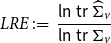 \begin{equation*} LRE \;:\!=\; \frac {\mathsf {ln\ } \mathsf {tr }\ \widehat {\Sigma }_v}{\mathsf {ln\ } \mathsf {tr }\ \Sigma _v} \end{equation*}
where $\widehat{\Sigma }_v = \Sigma _v$
is the best possible performance.
$\widehat{\Sigma }_v = \Sigma _v$
is the best possible performance.
3.1 Results
Our first simulation results are summarized in Table 1. It is clear that the superior performance of PWGC in comparison to AdaLASSO is as a result of limiting the false discovery rate. It is unsurprising that PWGC exhibits superior performance when the graph is an SCG, but even in the case of more general DAGs, the PWGC heuristic is still able to more reliably uncover the graph structure for small values of $q$
. We would conjecture that for small
$q$
. We would conjecture that for small $q$
, random graphs are “likely” to be “close” to SCGs in some appropriate sense. As
$q$
, random graphs are “likely” to be “close” to SCGs in some appropriate sense. As $q$
increases, there are simply not enough edges allowed by the SCG topology for it to be possible to accurately recover
$q$
increases, there are simply not enough edges allowed by the SCG topology for it to be possible to accurately recover $\mathcal{G}$
.
$\mathcal{G}$
.
Table 1. Simulation results—PWGC vs AdaLASSO
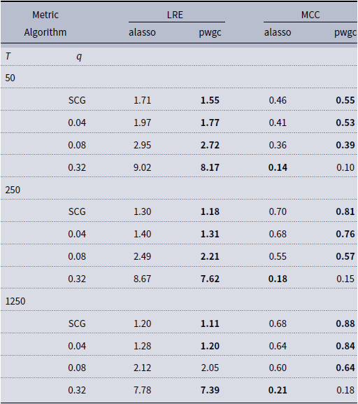
1. Results of Monte Carlo simulations comparing PWGC and AdaLASSO $(N = 50, p = 5, p_{\text{max}} = 10)$
for small samples and when the SCG assumption doesn’t hold. The superior result is bolded when the difference is statistically significant, as measured by scipy.stats.ttest_rel. 100 iterations are run for each set of parameters.
$(N = 50, p = 5, p_{\text{max}} = 10)$
for small samples and when the SCG assumption doesn’t hold. The superior result is bolded when the difference is statistically significant, as measured by scipy.stats.ttest_rel. 100 iterations are run for each set of parameters.
2. LRE: Log-Relative-Error, that is, the log sum of squared errors at each node relative to the strength of the driving noise $\frac{\mathsf{ln\ } \mathsf{tr } \widehat{\Sigma }_v}{\mathsf{ln\ } \mathsf{tr } \Sigma _v}$
. MCC: Matthew’s Correlation Coefficient.
$\frac{\mathsf{ln\ } \mathsf{tr } \widehat{\Sigma }_v}{\mathsf{ln\ } \mathsf{tr } \Sigma _v}$
. MCC: Matthew’s Correlation Coefficient.
3. Values of $q$
(edge probability) range between
$q$
(edge probability) range between $2/ N, 4/ N, 16/ N$
where
$2/ N, 4/ N, 16/ N$
where $2/ N$
has the property that the random graphs have on average the same number of edges as the SCG.
$2/ N$
has the property that the random graphs have on average the same number of edges as the SCG.
Figures 6 and 7 provide an empirical analysis of how the algorithm scales with increasing $N$
, and for a small number of training samples
$N$
, and for a small number of training samples $T$
. It is surprising that even for general DAGs (which don’t necessarily have the SCG property) performance degrades extremely slowly with respect to
$T$
. It is surprising that even for general DAGs (which don’t necessarily have the SCG property) performance degrades extremely slowly with respect to $N$
, and that performance is markedly better than random even when
$N$
, and that performance is markedly better than random even when $N \gt T$
. These observations are reminiscent of results for the LASSO algorithm applied to linear regression (Tibshirani et al., Reference Tibshirani, Wainwright and Hastie2015). For example, under certain conditions, it holds that
$N \gt T$
. These observations are reminiscent of results for the LASSO algorithm applied to linear regression (Tibshirani et al., Reference Tibshirani, Wainwright and Hastie2015). For example, under certain conditions, it holds that
 \begin{align*}||\hat {\beta }_{LASSO} - \beta ^\star ||_2^2 = \mathcal {O}\bigl (\frac {s}{T}\ \mathsf {ln\ } N\bigr ) \end{align*}
where $s$
is the number of non-zero parameters of
$s$
is the number of non-zero parameters of $\beta ^\star$
in the ground-truth linear regression model (Wainwright, Reference Wainwright2009).
$\beta ^\star$
in the ground-truth linear regression model (Wainwright, Reference Wainwright2009).
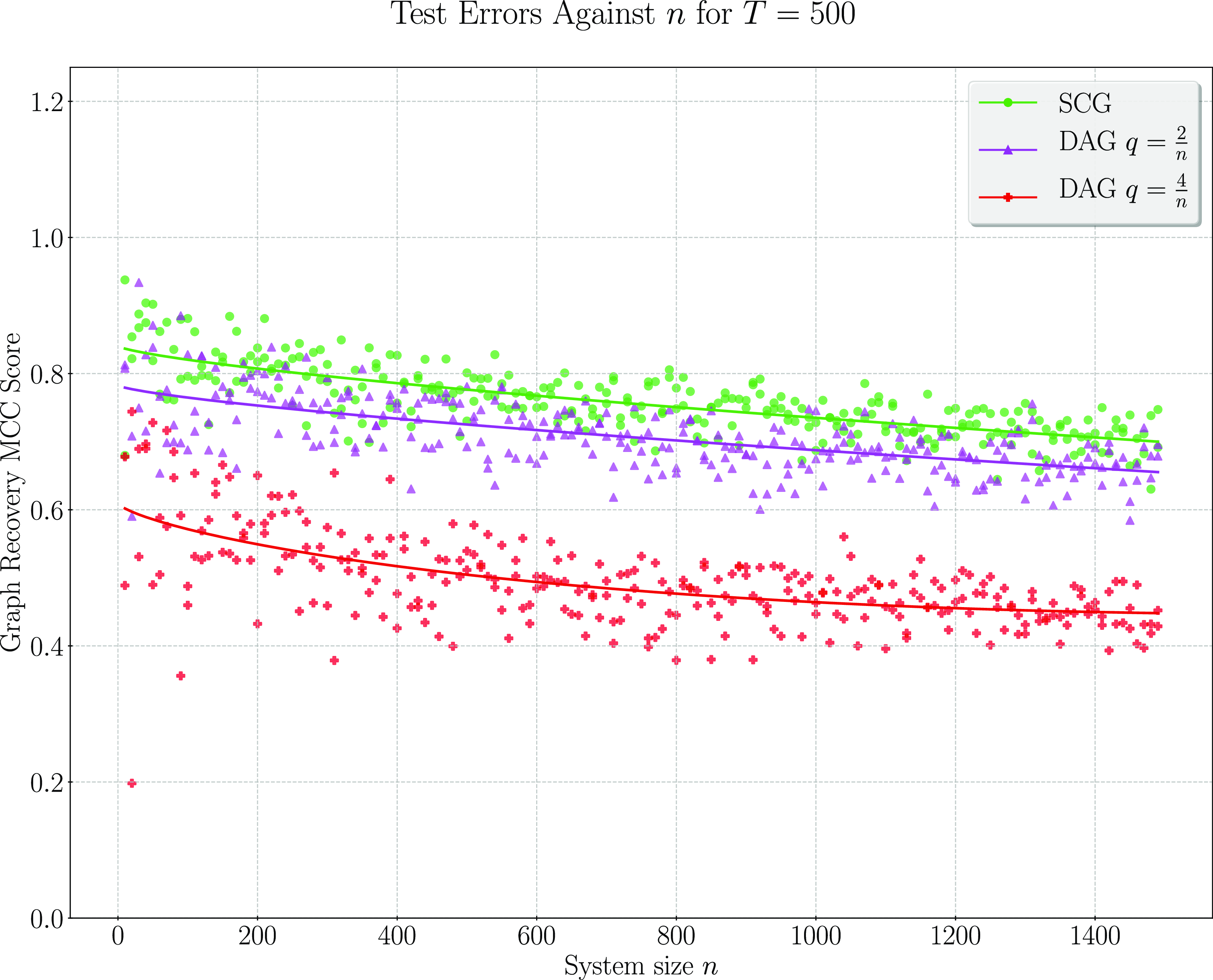
Figure 6. Measures support recovery performance as the number of nodes $N$
increases, and the edge proportion as well as the number of samples
$N$
increases, and the edge proportion as well as the number of samples $T$
is held fixed. Remarkably, the degradation as
$T$
is held fixed. Remarkably, the degradation as $N$
increases is limited, it is primarily the graph topology (SCG or non-SCG) as well as the level of sparsity (measured by
$N$
increases is limited, it is primarily the graph topology (SCG or non-SCG) as well as the level of sparsity (measured by $q$
) which are the determining factors for support recovery performance.
$q$
) which are the determining factors for support recovery performance.
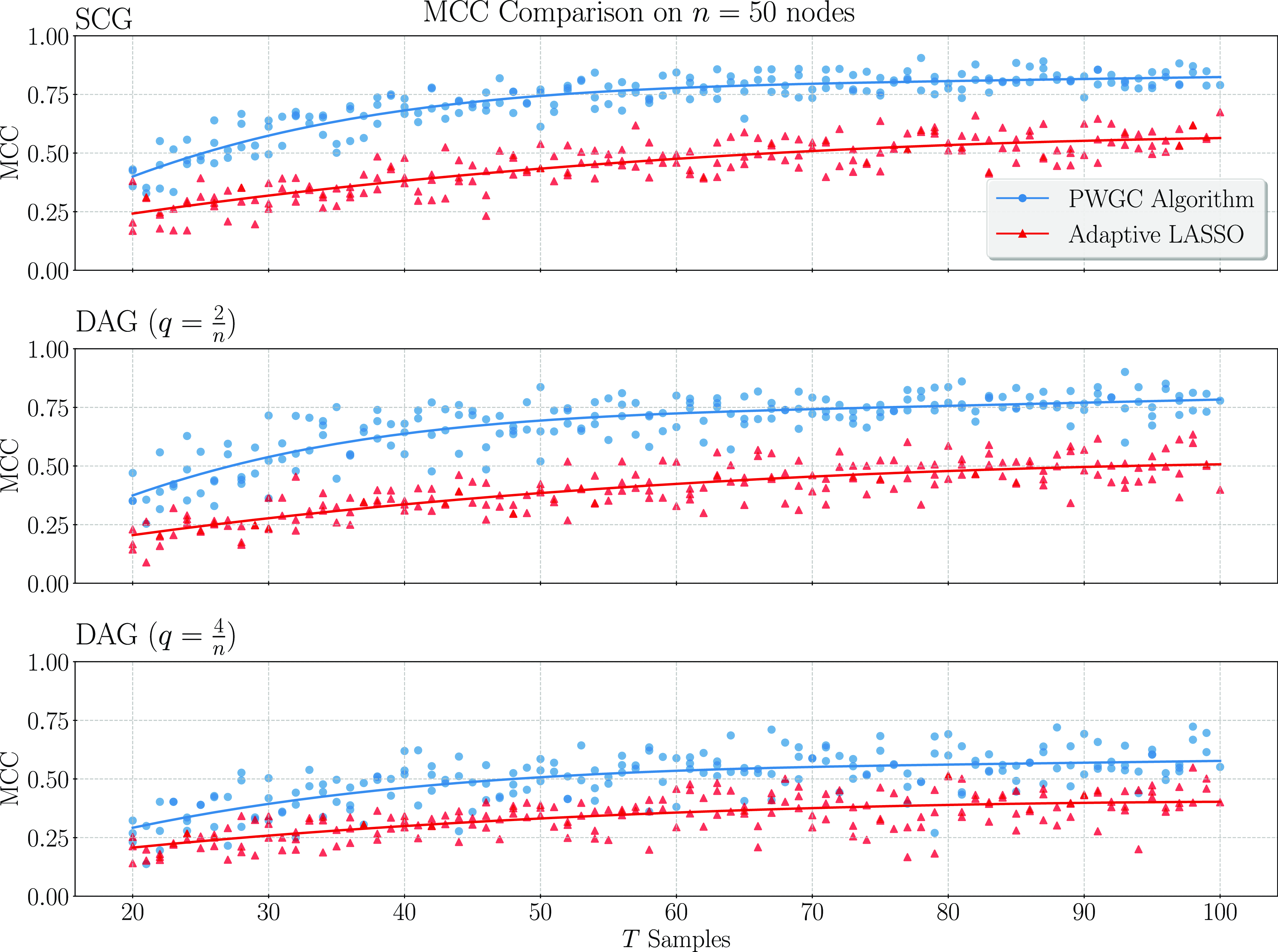
Figure 7. Provides a support recovery comparison for very small values of, $T$
typical for many applications. The system has a fixed number
$T$
typical for many applications. The system has a fixed number $N=50$
nodes.
$N=50$
nodes.
Additional experimental results, and a detailed description of the heuristic algorithm based on the theory of Section 2.7 is available in Appendix C.
4. Application example: Alcoholism classification from EEG networks
As was reviewed in the introduction to this paper, Granger causality analysis is frequently utilized for the analysis of brain connectivity networks in Neuroscience. This application is by now well established (Bressler & Seth, Reference Bressler and Seth2011), but is not without criticism. In particular, the critical paper of Haufe et al. (Reference Haufe, Nikulin, Müller and Nolte2013) states that “Many problems in neuroimaging (such as brain connectivity analysis) are inherently unsupervised, which means that the ’ground truth’ cannot be retrieved. In these cases, simulations are the only way to benchmark a method’s ability to solve the task if theoretical results are not available, while a neuroscientific finding on real data that matches prior expectations should not be mistaken for a proof-of-concept of the method.” This critical point has clear merit. Indeed, the motivation behind the simulation results of Section 3 is to apply our methodology to real data in a situation where we can identify the ground truth (since we constructed it), and therefore make certain types of comparisons between algorithms.
In the present application example, we challenge this dichotomy. We apply the Granger causality inference heuristic derived in this paper to construct estimates of signal space EEG causality networks for a large number of patients. A proportion of the patients in the data set have alcoholism, and we will show that, using only the inferred causality network, a logistic regression classifier can be constructed which discriminates between networks calculated from control subjects, and alcoholic subjects. The fact that it is possible to successfully perform this classification, at a rate better than random, is evidence that the Granger causality analysis detects and recovers consistent differences in the GCG networks of control and alcoholic EEG readings. This mode of analyzing the validity of a causality inference algorithm is a third method, conceptually distinct from the theory-or-simulation dichotomy identified by Haufe et al. (Reference Haufe, Nikulin, Müller and Nolte2013).
The data set we make use of was obtained from the “EEG Database Data Set”Footnote 3 (Zhang et al., Reference Zhang, Begleiter, Porjesz, Wang and Litke1995) from the UCI machine learning repository (Dua & Graff, Reference Dua and Graff2017). This data set contains 1 s long measurements of 64 channel EEG signals from patients who are given visual stimuli. The original data set contributors have filtered the frequencies of the recorded signals to lie between 0.02 and 50 Hz, and removed samples having excessive artifacts. As well as various important pre-processing steps particular to EEG data.
Precisely, the data set is described by
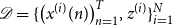 \begin{equation*}\mathcal {D} = \{\big (x^{(i)}(n)\big )_{n = 1}^T, z^{(i)} \}_{i = 1}^N\end{equation*}
where $T = 256$
,
$T = 256$
, $x^{(i)}(n) \in \mathbb{R}^{64}$
,
$x^{(i)}(n) \in \mathbb{R}^{64}$
, $z^{(i)} \in \{\mathsf{control}, \mathsf{alcoholic}\}$
, and
$z^{(i)} \in \{\mathsf{control}, \mathsf{alcoholic}\}$
, and
 N = 10,723
. That is,
N = 10,723
. That is, $x^{(i)}(n)$
is the EEG recordings of example
$x^{(i)}(n)$
is the EEG recordings of example $i$
, and
$i$
, and $z^{(i)}$
is a binary marker indicating the presence or absence of alcoholism in the subject. There are on average 90 trials for each subject, ranging between 30 and 119.
$z^{(i)}$
is a binary marker indicating the presence or absence of alcoholism in the subject. There are on average 90 trials for each subject, ranging between 30 and 119.
Applying a Granger causality inference algorithm to this data set results in a derivative data set $\widehat{\mathcal{D}} = \{A^{(i)}, z^{(i)}\}_{i = 1}^N$
, where
$\widehat{\mathcal{D}} = \{A^{(i)}, z^{(i)}\}_{i = 1}^N$
, where $A^{(i)} \in \{0, 1\}^{64 \times 64}$
is the adjacency matrix of the estimated causality network
$A^{(i)} \in \{0, 1\}^{64 \times 64}$
is the adjacency matrix of the estimated causality network $\widehat{\mathcal{G}}^{(i)}$
from example
$\widehat{\mathcal{G}}^{(i)}$
from example $i$
.
$i$
.
By fitting a classifier $\mathsf{clf}\;:\; \mathcal{G} \rightarrow \{\mathsf{control}, \mathsf{alcoholic}\}$
, which uses only the information available in the estimated causality network, we are able to make inference about whether or not the estimated causality graphs
$\mathsf{clf}\;:\; \mathcal{G} \rightarrow \{\mathsf{control}, \mathsf{alcoholic}\}$
, which uses only the information available in the estimated causality network, we are able to make inference about whether or not the estimated causality graphs $\widehat{\mathcal{G}}^{(i)}$
are uncovering relevant factors.
$\widehat{\mathcal{G}}^{(i)}$
are uncovering relevant factors.
4.1 Classifier methodology and evaluation
The classifier we apply is an off-the-shelf polynomial kernel logistic regression model: sklearn.linear_model.LogisticRegression (Pedregosa et al., Reference Pedregosa, Varoquaux, Gramfort, Michel, Thirion and Grisel2011), using a Nystroem kernel approximation (with 240 components): sklearn.kernel_approximation.Nystroem(kernel = ‘poly’). Hyperparameters are chosen via 10-fold cross validation with Bayesian Optimization (Kumar & Head, Reference Kumar and Head2017), using $80\%$
of the data. The remaining
$80\%$
of the data. The remaining $20\%$
of the data is held out for a final validation step. A polynomial kernel is natural for this task since the input features are binary (the adjacency matrix); a kernel degree of, say,
$20\%$
of the data is held out for a final validation step. A polynomial kernel is natural for this task since the input features are binary (the adjacency matrix); a kernel degree of, say, $3$
, indicates that graphical substructures no more complicated than triangles can be used by the classifier. Similarly to our simulation results, we use the MCC as the metric for evaluation.
$3$
, indicates that graphical substructures no more complicated than triangles can be used by the classifier. Similarly to our simulation results, we use the MCC as the metric for evaluation.
As a final verification, a label permutation test (“Test 1” in Ojala & Garriga (Reference Ojala and Garriga2010)) is applied to verify that $A^{(i)}$
and (
$A^{(i)}$
and ( $z^{(i)})$
are not independent, and to alleviate the fear that the classifier may simply be picking up on spurious patterns in the estimated causality graphs. This test consists of refit our classifier on randomly relabeled data and comparing the results those of the classifier fit on the correctly labeled data. An inability of the model to accurately discriminate between the labels in an incorrectly labeled data set is further evidence that accurate classification is not simply a result of overfitting or of picking up on spurious variation in the data
$z^{(i)})$
are not independent, and to alleviate the fear that the classifier may simply be picking up on spurious patterns in the estimated causality graphs. This test consists of refit our classifier on randomly relabeled data and comparing the results those of the classifier fit on the correctly labeled data. An inability of the model to accurately discriminate between the labels in an incorrectly labeled data set is further evidence that accurate classification is not simply a result of overfitting or of picking up on spurious variation in the data $A^{(i)}$
.
$A^{(i)}$
.
4.2 Results
The final value of the MCC for the alcoholism classification task, computed on a $10$
-fold cross validation is
$10$
-fold cross validation is $MCC = 0.305$
, with the individual folds falling into the interval
$MCC = 0.305$
, with the individual folds falling into the interval $[0.229, 0.396]$
. The MCC obtained on the final held-out validation set (i.e., data which was not used for picking any model parameters) was
$[0.229, 0.396]$
. The MCC obtained on the final held-out validation set (i.e., data which was not used for picking any model parameters) was $0.29$
. The p-value estimated from the label permutation test satisfies
$0.29$
. The p-value estimated from the label permutation test satisfies $p \lt 0.01$
and where the average MCC obtained on the validation data, by the 100 classifiers fit on data with randomly permuted labels, was zero through two decimal places. While the performance of the classifier is not exemplary, these results establish clearly that the performance is statistically significantly better than random.
$p \lt 0.01$
and where the average MCC obtained on the validation data, by the 100 classifiers fit on data with randomly permuted labels, was zero through two decimal places. While the performance of the classifier is not exemplary, these results establish clearly that the performance is statistically significantly better than random.
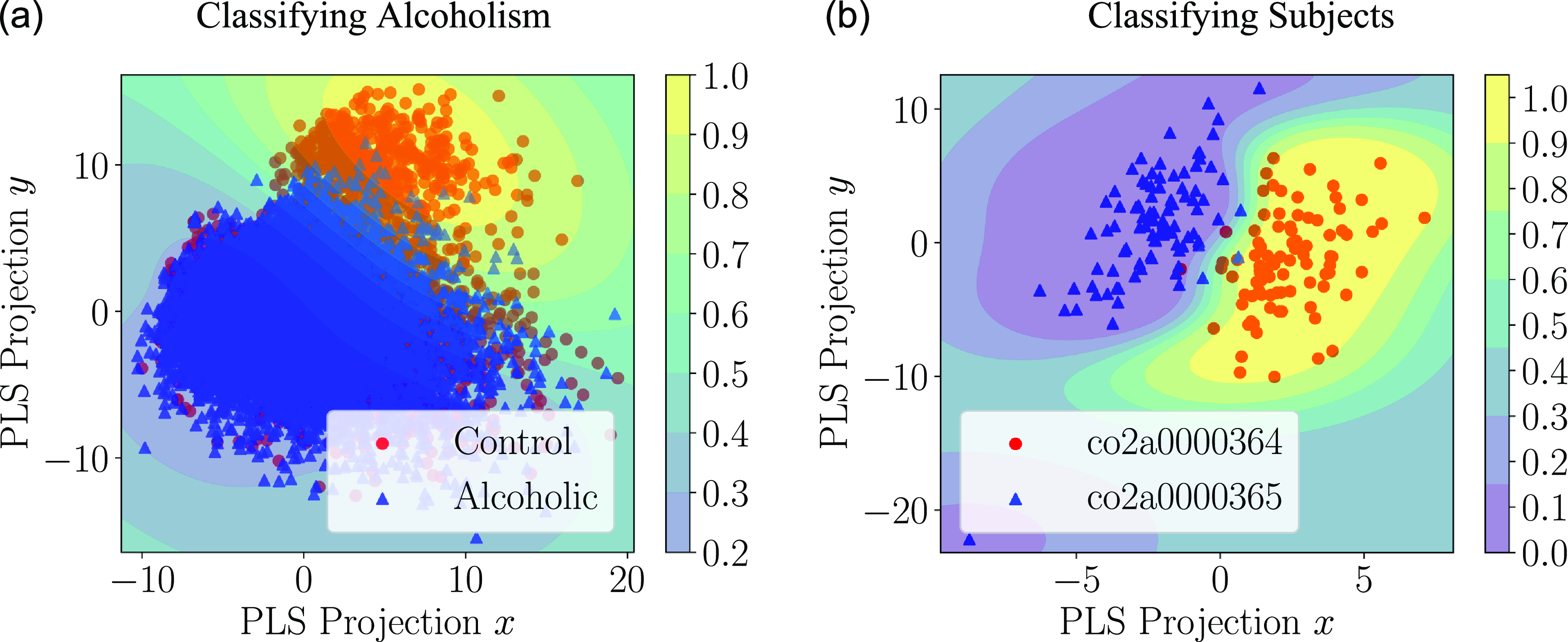
Figure 8. Is a low-dimensional embedding representing the classification of alcoholic and non-alcoholic subjects based entirely on the Granger causality graphs constructed from EEG signals. Figure 8b further illustrates a classification task using EEG causality graphs. In this case, one particular subject can be almost perfectly separated from another particular subject with a binary classifier. These results indicate the causality graph carries consistent and identifiable cross-subject patterns.
The EEG alcoholism data set has other potential classification labels. One natural example is to classify the subject label. That is, to identify the subject to which the EEG example belongs (each subject had multiple EEG recordings taken). We do not report the details as the task is considerably easier and the methodology is similar to that described in Section 4.1. However, a classifier trained on any two specific subjects is able to discern out-of-sample causality graphs between the two subjects with almost perfect accuracy. Specifically, we obtained an MCC of $0.99$
and the p-value estimated by a permutation test satisfied
$0.99$
and the p-value estimated by a permutation test satisfied $p \lt 0.001$
.
$p \lt 0.001$
.
An illustration of the alcoholism classifier, as well as a particular example from the subject-subject classifier is provided in Figure 8. The visualization is constructed by projecting onto two basis dimensions by partial least squares (a supervised dimensionality reduction technique). These visualizations are provided entirely for qualitative context, but drawing substantive conclusions from them is not appropriate. In particular, the low-dimensional visualization does not necessarily accurately capture the high-dimensional decision surface utilized by the classifiers.
5. Conclusion
We have argued that considering particular topological properties of Granger causality networks can provide substantial insights into the structure of causality graphs with potential for providing improvements to causality graph estimation when structural assumptions are met. In particular, the notion of a strongly causal graph has been exploited to establish conditions under which pairwise causality testing alone is sufficient for recovering a complete Granger causality graph. Moreover, examples from the literature suggest that such topological assumptions may be reasonable in some applications. And secondly, even when the strong causality assumption is not met, we have provided simulation evidence to suggest that our pairwise testing algorithm PWGC can still outperform the LASSO and adaLASSO, both of which are commonly employed in applications.
In addition to this simulation study, we have constructed an application example using EEG data. In this example, we use off-the-shelf machine learning classifiers to detect the presence or absence of alcoholism based entirely upon the Granger causality graph topology. While this alcoholism classification task is quite challenging, we demonstrate that classifying between distinct subjects in the study, again based only upon the inferred Granger causality graphs, is easy: such classifiers can obtain nearly $100\%$
accuracy. This evidence demonstrates that consistent and meaningful features are being extracted by the Granger causality analysis.
$100\%$
accuracy. This evidence demonstrates that consistent and meaningful features are being extracted by the Granger causality analysis.
We emphasize that the causality graph topology is one of the key defining features of time series analysis in comparison to standard multivariate regression and therefore advocate for further study of how different topological assumptions may impact the recovery of causality graphs.
Competing interests
None.
Supplementary materials
For supplementary material for this article, please visit http://doi.org/10.1017/nws.2023.11


 Open access