


1. Introduction
The field of statistical modeling and analysis of complex networks has gained increasing interest over the last two decades. This is driven by the fact that different types of systems can be reasonably formalized as relationships between individuals or interactions between objects. Analyzing such structures consequently allows to uncover and describe the phenomena that affect these systems. Network-structured data arise in various fields, for example, social and political sciences, economics, biology, and neurosciences, to name but a few. In this regard, a connectivity pattern between entities might describe friendships among members of a social group (Eagle et al., Reference Eagle, Pentland and Lazer2009), the trading between nations (Bhattacharya et al., Reference Bhattacharya, Mukherjee, Saramäki, Kaski and Manna2008), interactions of proteins (Schwikowski et al., Reference Schwikowski, Uetz and Fields2000), or the functional coactivation within the human brain (Bassett et al., Reference Bassett, Zurn and Gold2018, Crossley et al., Reference Crossley, Mechelli, Vértes, Winton-Brown, Patel, Ginestet and Bullmore2013).
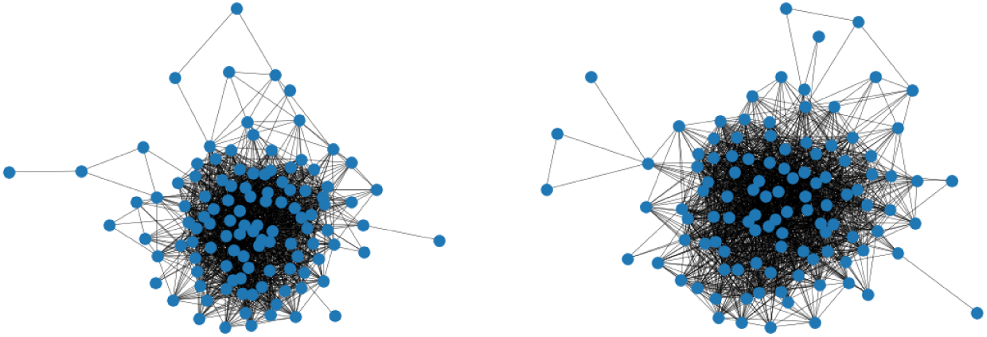
In many situations, uncovering the underlying connectivity structure is not the only concern but also the comparison of akin networks and the exploration of potential differences. For instance, this might be of interest in the context of brain coactivation, which we consider here as motivating example. Recently, a lot of work has been going on investigating how the functional connectivity in the brain differs when people are affected by cognitive disorders like Alzheimer’s disease or autism spectrum disorder (Song et al., Reference Song, Epalle and Lu2019, Subbaraju et al., Reference Subbaraju, Suresh, Sundaram and Narasimhan2017, Pascual-Belda et al., Reference Pascual-Belda, Díaz-Parra and Moratal2018). Two such functional coactivation networks—resulting from averaging over the measurements within two different subject groups, respectively—are illustrated in Figure 1. One inquiry which is then particularly relevant to the research question posed is whether a significant difference can be observed in these brain processes. More generally, this can be phrased as a hypothesis test on structural equivalence of two networks as exemplarily raised for the situation in Figure 1.
Functional coactivation networks of the human brain. The illustrated connectivity patterns result from averaging over multiple measurements for subjects with autism spectrum disorder (left) and typical development (right). Do these networks reveal a significant structural difference?.
To this end, we pursue constructing a statistical approach for network comparison that allows for a conclusion about significance. More precisely, we aim to test whether two networks can be considered as independent samples drawn from the same probability distribution. This is apparently in itself a technically difficult question since the two networks can have different sizes, and hence the two distributions need to be somehow different. Therefore, it is crucial that the applied distributional framework constitutes a rather universal probability measure. In fact, this is not a trivial property, and many network models entail conceptual issues that impede a direct comparison. For example, in the Exponential Random Graph Model (Robins et al., Reference Robins, Pattison, Kalish and Lusher2007), a concrete model parameterization has different implications for different network sizes, making corresponding coefficient estimates hardly comparable. Hence, for the given research question, statistical models seem advantageous where the specification of size and edge probabilities can be explicitly disentangled.
For such a comparative analysis of networks, we will demonstrate that Graphon Models (Lovász and Szegedy, Reference Lovász and Szegedy2006, Diaconis and Janson, Reference Diaconis and Janson2008, Sischka and Kauermann, Reference Sischka and Kauermann2022) are a very useful tool. First, the graphon model is very flexible and able to capture complex network structures. Secondly, the graphon itself can be interpreted as local density or intensity function on networks of nonparametric fashion. Lastly, the model’s design fulfills the above requirement of decoupling the network’s structure and size, allowing for modeling multiple networks simultaneously (Navarro and Segarra, Reference Navarro and Segarra2022). Hence, the graphon framework appears as a natural choice for comparison purposes.
The rest of the paper is organized as follows. In Section 2, we start with reviewing methods from the network comparison literature. A formalization of the test problem is elaborated and discussed in Section 3. Section 4 then deals with the joint graphon estimation, which is essential for the testing procedure to be applicable. Based on the joint graphon model, in Section 5, we develop a network comparison strategy for testing on equivalence of the underlying structures. The general applicability of the complete approach is demonstrated in Section 6, where we consider its performance on simulated and real-world data. The discussion and conclusion in Section 7 complete the paper.
2. Concepts for network comparison
When it comes to the comparison of networks, as a first step, one needs to decide on a concept for specifying network structures. In general, the various approaches can be broadly distinguished according to whether they rely on a descriptive or a model-based structural framework. Survey articles in this field are given by Soundarajan et al., (Reference Soundarajan, Eliassi-Rad and Gallagher2014), Yaveroğlu et al., (Reference Yaveroğlu, Milenković and Pržulj2015), Emmert-Streib et al., (Reference Emmert-Streib, Dehmer and Shi2016), and Tantardini et al., (Reference Tantardini, Ieva, Tajoli and Piccardi2019). A more general perspective on how complex data objects—such as adjacency matrices—might be compared is pointed out by Marron and Alonso (Reference Marron and Alonso2014). Looking into the aforementioned compendia and examining the general literature on network comparison, however, reveals a lack of model-based comparison approaches. This can also be seen in the following, where we briefly review the different strategies that have been proposed so far.
Starting with approaches that are based on extracted network statistics, the most intuitive strategy is presumably to simply compare global characteristics such as the clustering coefficient or the average path length (Newman, Reference Newman2018, pp. 364 ff., Butts Reference Butts2008, p. 31). An extensive analysis on the capability of common network metrics in the setting of monitoring and identifying differences in dynamic network structures has been carried out by Flossdorf and Jentsch (Reference Flossdorf and Jentsch2021). However, a single feature captures the overall network structure in most cases only very poorly since networks that are structured completely differently can apparently still possess a very similar value for that global statistic. Flossdorf et al., (Reference Flossdorf, Fried and Jentsch2023) tackle this issue by using multiple metrics. Aiming in a similar direction, Wilson and Zhu (Reference Wilson and Zhu2008) consider the differences in the graph spectra, see also Gera et al., (Reference Gera, Alonso, Crawford, House, Mendez-Bermudez, Knuth and Miller2018). Yet, for the spectrum, it is often unclear which information in terms of local structural properties is extracted from the network and hence such approaches somehow ascribe only too little importance to the attributes of interest.
Another branch of the literature on descriptive network comparison relies on the concept of graphlets, i.e. prespecified subgraph patterns that are assumed to be sufficient for describing the present structure. Papers that, in one way or another, consider differences in the frequencies of graphlets are, among others, Pržulj et al., (Reference Pržulj, Corneil and Jurisica2004), Pržulj (Reference Pržulj2007), Ali et al., (Reference Ali, Rito, Reinert, Sun and Deane2014), and Faisal et al., (Reference Faisal, Newaz, Chaney, Li, Emrich, Clark and Milenković2017). Since the counting procedure is rather complex for larger graphlets, it is sort of a consensus to include only those that consist of no more than five nodes. Apparently, this seems somehow arbitrary and incomplete in terms of capturing all structural aspects. Moreover, Yaveroğlu et al., (Reference Yaveroğlu, Malod-Dognin, Davis, Levnajic, Janjic, Karapandza, Stojmirovic and Pržulj2014) found high correlations among the graphlet-related statistics, including complete redundancies. On the other hand, a connection between subgraph frequencies and the concrete specification of the graphon model is exemplarily elaborated in Borgs et al., (Reference Borgs, Chayes, Lovász, Sós and Vesztergombi2008), Bickel et al., (Reference Bickel, Chen and Levina2011), and Latouche and Robin (Reference Latouche and Robin2016).
Despite their wide dissemination, descriptive network statistics entail two general shortcomings. First, it is very difficult to assess which network segments accommodate the structural key differences. To be precise, the nodes or edges (present or absent) that contribute most to a quantified structural discrepancy can only hardly be detected. Secondly, drawing inference on the dissimilarity of two networks based on multiple network statistics is a complex inferential problem. For example, Butts (Reference Butts2008) aims to overcome this deficit by applying a simplistic conditional uniform graph distribution.
On the other hand, probabilistic models for network data induce distributions on structural patterns that extend to desired distributional assumptions on structural differences. As a consequence, these modeling frameworks might provide concepts for network comparison. Yet, due to a certain level of model complexity, which is required to adequately represent inherently complex network data, individual shortcomings are entailed that often prevent a direct comparison. While, for example, the Latent Distance Model (Hoff et al., Reference Hoff, Raftery and Handcock2002) does not yield any model-related key component to be compared, coefficient estimates from the exponential random graph model are not directly comparable across separated networks. The graphon model and the Stochastic Blockmodel (see Holland et al., Reference Holland, Laskey and Leinhardt1983 and Snijders and Nowicki, Reference Snijders and Nowicki1997 and Reference Nowicki and Snijders2001) suffer from identifiability issues (Diaconis and Janson, Reference Diaconis and Janson2008, Thm. 7.1 ) that make a comparison of corresponding individual estimates very complicated. The blockmodel’s adaptivity is additionally highly dependent on the choice of the number of blocks. Onnela et al., (Reference Onnela, Fenn, Reid, Porter, Mucha, Fricker and Jones2012) tackle this issue by observing the networks’ complete disintegration processes, which they describe by the profiles over well-known network statistics. Appropriately summarizing the differences in these profiles has been demonstrated to provide a reasonable distance measure between networks that leads to good classification.
Overall, in view of the issues mentioned above, it seems little surprising that the literature on model-based strategies for network comparison is rather scant. More specifically, to the best of our knowledge, there exists no nonparametric statistical test on the equivalence of network structures. This shortcoming is what we aim to address in this paper. To do so, we formulate a joint smooth graphon framework that can subsequently be used for constructing an appropriate testing procedure.
3. Notation and formulation of the test problem
We consider the setting where two undirected networks of sizes $N^{(1)}$
and
$N^{(1)}$
and $N^{(2)}$
have been observed. Let
$N^{(2)}$
have been observed. Let $\boldsymbol{y}^{(g)} = [y_{ij}^{(g)}]_{i,j = 1, \ldots , N^{(g)}}$
for
$\boldsymbol{y}^{(g)} = [y_{ij}^{(g)}]_{i,j = 1, \ldots , N^{(g)}}$
for $g =1, 2$
denote the two respective adjacency matrices, where
$g =1, 2$
denote the two respective adjacency matrices, where $y_{ij}^{(g)} = 1$
if, in network
$y_{ij}^{(g)} = 1$
if, in network $g$
, there exists an edge between nodes
$g$
, there exists an edge between nodes $i$
and
$i$
and $j$
and
$j$
and $y^{(g)}_{ij}=0$
otherwise. Since we assume the networks to be undirected, this specifically means that
$y^{(g)}_{ij}=0$
otherwise. Since we assume the networks to be undirected, this specifically means that $y_{ij}^{(g)} = y_{ji}^{(g)}$
, leading to a symmetric
$y_{ij}^{(g)} = y_{ji}^{(g)}$
, leading to a symmetric $\boldsymbol{y}^{(g)} \in \{0,1\}^{N^{(g)} \times N^{(g)}}$
. Additionally, for the diagonal elements, we set
$\boldsymbol{y}^{(g)} \in \{0,1\}^{N^{(g)} \times N^{(g)}}$
. Additionally, for the diagonal elements, we set $y_{ii}^{(g)}=0$
, reflecting the absence of self-loops. In general, we consider
$y_{ii}^{(g)}=0$
, reflecting the absence of self-loops. In general, we consider $\boldsymbol{y}^{(g)}$
to be a realization of a random network
$\boldsymbol{y}^{(g)}$
to be a realization of a random network $\boldsymbol{Y}^{(g)}$
of size
$\boldsymbol{Y}^{(g)}$
of size $N^{(g)}$
which is subject to probability mass
$N^{(g)}$
which is subject to probability mass $\mathbb{P}(\boldsymbol{Y}^{(g)} = \boldsymbol{y}^{(g)} \, ; N^{(g)})$
. The question we aim to tackle is whether
$\mathbb{P}(\boldsymbol{Y}^{(g)} = \boldsymbol{y}^{(g)} \, ; N^{(g)})$
. The question we aim to tackle is whether $\boldsymbol{y}^{(1)}$
and
$\boldsymbol{y}^{(1)}$
and $\boldsymbol{y}^{(2)}$
are drawn from the same distribution. To suitably specify such a distribution, we rely on the smooth graphon model. The data-generating process is thereby as follows. Assume that we independently draw uniformly distributed random variables
$\boldsymbol{y}^{(2)}$
are drawn from the same distribution. To suitably specify such a distribution, we rely on the smooth graphon model. The data-generating process is thereby as follows. Assume that we independently draw uniformly distributed random variables
 \begin{equation} U^{(g)}_i \sim \mbox{Uniform}[0,1] \quad \mbox{for } i = 1, \ldots , N^{(g)} \mbox{ and } g= 1,2. \end{equation}
Conditional on ${\boldsymbol{U}}^{(g)}=(U^{(g)}_1, \ldots , U_{N^{(g)}}^{(g)})$
, we then draw the edges i.i.d. through
${\boldsymbol{U}}^{(g)}=(U^{(g)}_1, \ldots , U_{N^{(g)}}^{(g)})$
, we then draw the edges i.i.d. through
 \begin{equation} Y_{ij}^{(g)} \mid ({\boldsymbol{U}}^{(g)} = {\boldsymbol{u}}^{(g)} ) \sim \mbox{Binomial}(1 , w^{(g)}(u^{(g)}_i , u^{(g)}_j ) ) \quad \mbox{for } j\gt i \end{equation}
with ${\boldsymbol{u}}^{(g)}=(u^{(g)}_1, \ldots , u_{N^{(g)}}^{(g)}) \in [0,1]^{N^{(g)}}$
and under the setting of
${\boldsymbol{u}}^{(g)}=(u^{(g)}_1, \ldots , u_{N^{(g)}}^{(g)}) \in [0,1]^{N^{(g)}}$
and under the setting of $Y_{ij}^{(g)} \equiv Y_{ji}^{(g)}$
for
$Y_{ij}^{(g)} \equiv Y_{ji}^{(g)}$
for $j\lt i$
and
$j\lt i$
and $Y_{ii}^{(g)} \equiv 0$
. The function
$Y_{ii}^{(g)} \equiv 0$
. The function $w^{(g)}: [0,1]^2 \rightarrow [0,1]$
is called graphon (see Lovász and Szegedy, Reference Lovász and Szegedy2006 and Diaconis and Janson, Reference Diaconis and Janson2008). We assume
$w^{(g)}: [0,1]^2 \rightarrow [0,1]$
is called graphon (see Lovász and Szegedy, Reference Lovász and Szegedy2006 and Diaconis and Janson, Reference Diaconis and Janson2008). We assume $w^{(g)}(\cdot ,\cdot )$
to be smooth according to some Hölder or Lipschitz condition (cf. Wolfe and Olhede, Reference Wolfe and Olhede2013 or Chan and Airoldi, Reference Chan and Airoldi2014). Relying on this data-generating process, the graphon-based probability model can be defined through
$w^{(g)}(\cdot ,\cdot )$
to be smooth according to some Hölder or Lipschitz condition (cf. Wolfe and Olhede, Reference Wolfe and Olhede2013 or Chan and Airoldi, Reference Chan and Airoldi2014). Relying on this data-generating process, the graphon-based probability model can be defined through
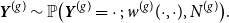 \begin{equation} \boldsymbol{Y}^{(g)} \sim \mathbb{P}\big (\boldsymbol{Y}^{(g)} = \cdot \, ; \, w^{(g)}(\cdot , \cdot ) , N^{(g)}\big ). \end{equation}
In this distribution model, the network’s size and structure are apparently dissociated, which therefore allows for a size-independent comparison of underlying structures. Hence, our goal is to develop a statistical test on the hypothesis
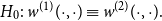 \begin{equation} H_0 : \; w^{(1)}(\cdot , \cdot ) \equiv w^{(2)}(\cdot , \cdot ). \end{equation}
In this context, we emphasize that data-generating process (2) is not unique because it is invariant to permutations of $w^{(g)}(\cdot ,\cdot )$
, as discussed in detail by Diaconis and Janson(2008, Sec. 7). Thus, the formulation of
$w^{(g)}(\cdot ,\cdot )$
, as discussed in detail by Diaconis and Janson(2008, Sec. 7). Thus, the formulation of $H_0$
needs to be formally understood from the perspective of corresponding equivalence classes. For the concrete implementation of the test procedure, we employ a concrete representation of the two graphons as described below. Specifically, under the assumption of
$H_0$
needs to be formally understood from the perspective of corresponding equivalence classes. For the concrete implementation of the test procedure, we employ a concrete representation of the two graphons as described below. Specifically, under the assumption of $H_0$
, we define the joint graphon
$H_0$
, we define the joint graphon
 \begin{equation*} w^{\text{joint}}(u,v) \,:\!=\, w^{(1)}(u, v) = w^{(2)}(u, v) \quad \mbox{for all } (u,v)^\top \in [0,1]^2. \end{equation*}
Since $w^{(1)}(\cdot ,\cdot )$
and
$w^{(1)}(\cdot ,\cdot )$
and $w^{(2)}(\cdot ,\cdot )$
are assumed to be smooth, this also holds for
$w^{(2)}(\cdot ,\cdot )$
are assumed to be smooth, this also holds for $w^{\text{joint}}(\cdot ,\cdot )$
. Given such joint graphon, the node position vectors
$w^{\text{joint}}(\cdot ,\cdot )$
. Given such joint graphon, the node position vectors ${\boldsymbol{u}}^{(1)}$
and
${\boldsymbol{u}}^{(1)}$
and ${\boldsymbol{u}}^{(2)}$
referring to
${\boldsymbol{u}}^{(2)}$
referring to $w^{\text{joint}}(\cdot ,\cdot )$
then provide a specific type of network alignment. This is what we utilize for a direct comparison of
$w^{\text{joint}}(\cdot ,\cdot )$
then provide a specific type of network alignment. This is what we utilize for a direct comparison of $\boldsymbol{y}^{(1)}$
and
$\boldsymbol{y}^{(1)}$
and $\boldsymbol{y}^{(2)}$
. Having said that, in real-world applications, neither (
$\boldsymbol{y}^{(2)}$
. Having said that, in real-world applications, neither ( ${\boldsymbol{u}}^{(1)}, {\boldsymbol{u}}^{(2)}$
) nor
${\boldsymbol{u}}^{(1)}, {\boldsymbol{u}}^{(2)}$
) nor $w^{\text{joint}}(\cdot ,\cdot )$
is observed. Thus, in order to achieve this alignment, we first need to formulate an appropriate estimation procedure for the joint graphon model. Note that, strictly speaking, according to formulation (3) this requires the presence of dense networks. Yet, the following modeling technique and the subsequent testing procedure are reasonable if the empirical densities are high enough and the observed networks are considered to be fixed in
$w^{\text{joint}}(\cdot ,\cdot )$
is observed. Thus, in order to achieve this alignment, we first need to formulate an appropriate estimation procedure for the joint graphon model. Note that, strictly speaking, according to formulation (3) this requires the presence of dense networks. Yet, the following modeling technique and the subsequent testing procedure are reasonable if the empirical densities are high enough and the observed networks are considered to be fixed in $N^{(g)}$
,
$N^{(g)}$
, $g=1,2$
.
$g=1,2$
.
4. EM-based joint graphon estimation
In this section, we present an iterative estimation procedure for the joint smooth graphon model under the assumption that null hypothesis (4) is true. To do so, we follow the EM-based estimation routine of Sischka and Kauermann (Reference Sischka and Kauermann2022), extending it to the situation of two networks.
4.1 MCMC E-step
Starting with the E-step of our iterative algorithm, we assume the joint graphon $w^{\text{joint}}(\cdot , \cdot )$
to be known for the moment. Based on that, the latent positions of the networks can be separately determined using MCMC techniques. To be precise, we apply Gibbs sampling by formulating the full conditional distribution of
$w^{\text{joint}}(\cdot , \cdot )$
to be known for the moment. Based on that, the latent positions of the networks can be separately determined using MCMC techniques. To be precise, we apply Gibbs sampling by formulating the full conditional distribution of $U_i^{(g)}$
through
$U_i^{(g)}$
through
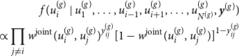 \begin{align} f(u_i^{(g)} \mid u_1^{(g)},\ldots , u_{i-1}^{(g)},u_{i+1}^{(g)}, \ldots , u_{N^{(g)}}^{(g)}, \boldsymbol{y}^{(g)}) \nonumber \\ \propto \prod _{j \neq i} w^{\text{joint}}(u_i^{(g)} , u_j^{(g)})^{y_{ij}^{(g)}} [1 - w^{\text{joint}}(u_i^{(g)} , u_j^{(g)})]^{1-{y_{ij}^{(g)}}} \end{align}
for all $i = 1,\ldots , N^{(g)}$
and
$i = 1,\ldots , N^{(g)}$
and $g=1, 2$
. Details on the concrete implementation of the Gibbs sampler are given in Section A of the Appendix. The resulting MCMC sequence (after cutting the burn-in period and appropriate thinning) then reflects the joint conditional distribution
$g=1, 2$
. Details on the concrete implementation of the Gibbs sampler are given in Section A of the Appendix. The resulting MCMC sequence (after cutting the burn-in period and appropriate thinning) then reflects the joint conditional distribution $f({\boldsymbol{u}}^{(g)} \mid \boldsymbol{y}^{(g)})$
. Thus, the marginal conditional means of the latent positions, i.e.
$f({\boldsymbol{u}}^{(g)} \mid \boldsymbol{y}^{(g)})$
. Thus, the marginal conditional means of the latent positions, i.e. $\mathbb{E} (U_i^{(g)} \mid \boldsymbol{Y}^{(g)} = \boldsymbol{y}^{(g)})$
for
$\mathbb{E} (U_i^{(g)} \mid \boldsymbol{Y}^{(g)} = \boldsymbol{y}^{(g)})$
for $i=1,\ldots ,N^{(g)}$
, can be approximated by taking the mean over the MCMC samples, which we denote by
$i=1,\ldots ,N^{(g)}$
, can be approximated by taking the mean over the MCMC samples, which we denote by $\bar {{\boldsymbol{u}}}^{(g)} = (\bar {u}_1^{(g)}, \ldots , \bar {u}_{N^{(g)}}^{(g)})$
. This posterior mean vector, however, requires further adjustment due to additional identifiability issues that cannot be coped with by the standard EM-type algorithm. To illustrate this, let model assumption (1) be more relaxed in the sense that the
$\bar {{\boldsymbol{u}}}^{(g)} = (\bar {u}_1^{(g)}, \ldots , \bar {u}_{N^{(g)}}^{(g)})$
. This posterior mean vector, however, requires further adjustment due to additional identifiability issues that cannot be coped with by the standard EM-type algorithm. To illustrate this, let model assumption (1) be more relaxed in the sense that the $U_i^{(g)}$
’s are assumed to follow a continuous distribution
$U_i^{(g)}$
’s are assumed to follow a continuous distribution $F^{(g)}(\cdot )$
. Under this configuration, the model (
$F^{(g)}(\cdot )$
. Under this configuration, the model ( $F^{(g)}(\cdot )$
,
$F^{(g)}(\cdot )$
, $w^{(g)}(\cdot ,\cdot )$
) is equivalent to any other model (
$w^{(g)}(\cdot ,\cdot )$
) is equivalent to any other model ( ${F^{(g)}}^\prime (\cdot )$
,
${F^{(g)}}^\prime (\cdot )$
, ${w^{(g)}}^\prime (\cdot ,\cdot )$
) constructed through
${w^{(g)}}^\prime (\cdot ,\cdot )$
) constructed through
 \begin{equation*} {F^{(g)}}^\prime (u^\prime ) \,:\!=\, F^{(g)}(\varphi (u^\prime )) \quad \mbox{and} \quad {w^{(g)}}^\prime (u^\prime ,v^\prime ) \,:\!=\, w^{(g)} (\varphi (u^\prime ),\varphi (v^\prime )) \end{equation*}
with $\varphi : [0,1] \rightarrow [0,1]$
being a strictly increasing continuous function (that is, in contrast to Diaconis and Janson, Reference Diaconis and Janson2008, Sec. 7 not measure-preserving). Specifically, that means
$\varphi : [0,1] \rightarrow [0,1]$
being a strictly increasing continuous function (that is, in contrast to Diaconis and Janson, Reference Diaconis and Janson2008, Sec. 7 not measure-preserving). Specifically, that means
 \begin{equation*} \mathbb{P}\big (\boldsymbol{Y}^{(g)} = \cdot \, ; \, F^{(g)}(\cdot ), w^{(g)}(\cdot ,\cdot ) , N^{(g)}\big ) \equiv \mathbb{P}\big (\boldsymbol{Y}^{(g)} = \cdot \, ; \, {F^{(g)}}^\prime (\cdot ), {w^{(g)}}^\prime (\cdot ,\cdot ) , N^{(g)}\big ) \end{equation*}
for all $N^{(g)} \geq 2$
. As a matter of conception, this issue cannot be solved by the EM algorithm since it aims at specifying a model that adapts optimally to the given data instead of perfectly recovering the underlying model structure. Consequently, the EM approach is not able to distinguish between the two conceptually equivalent model specifications (
$N^{(g)} \geq 2$
. As a matter of conception, this issue cannot be solved by the EM algorithm since it aims at specifying a model that adapts optimally to the given data instead of perfectly recovering the underlying model structure. Consequently, the EM approach is not able to distinguish between the two conceptually equivalent model specifications ( $F^{(g)}(\cdot )$
,
$F^{(g)}(\cdot )$
, $w^{(g)}(\cdot ,\cdot )$
) and (
$w^{(g)}(\cdot ,\cdot )$
) and ( ${F^{(g)}}^\prime (\cdot )$
,
${F^{(g)}}^\prime (\cdot )$
, ${w^{(g)}}^\prime (\cdot ,\cdot )$
). Nonetheless, this identifiability issue can simply be tackled by adjusting
${w^{(g)}}^\prime (\cdot ,\cdot )$
). Nonetheless, this identifiability issue can simply be tackled by adjusting $\bar {{\boldsymbol{u}}}^{(g)}$
before estimating the graphon in the M-step. To do so, we just impose that the inferred node positions follow an ideal sample drawn from the standard uniform distribution and thus intend to sprawl out the posterior means in an equidistant manner. More precisely, as an order-preserving adjusted estimate that is directly derived from the Gibbs sampler we utilize the “uniformized” posterior mean
$\bar {{\boldsymbol{u}}}^{(g)}$
before estimating the graphon in the M-step. To do so, we just impose that the inferred node positions follow an ideal sample drawn from the standard uniform distribution and thus intend to sprawl out the posterior means in an equidistant manner. More precisely, as an order-preserving adjusted estimate that is directly derived from the Gibbs sampler we utilize the “uniformized” posterior mean
 \begin{equation*} \hat {u}_i^{(g)} = \frac {\operatorname {rank} (\bar {u}_i^{(g)})}{N^{(g)}+1}, \end{equation*}
where $\operatorname {rank}(\bar {u}_i^{(g)})$
is the rank from the smallest to the largest of element
$\operatorname {rank}(\bar {u}_i^{(g)})$
is the rank from the smallest to the largest of element $\bar {u}_i^{(g)}$
within
$\bar {u}_i^{(g)}$
within $\bar {{\boldsymbol{u}}}^{(g)}$
. In this context, note that the values
$\bar {{\boldsymbol{u}}}^{(g)}$
. In this context, note that the values $i/(N^{(g)}+1)$
with
$i/(N^{(g)}+1)$
with $i=1,\ldots ,N^{(g)}$
represent the expectations of
$i=1,\ldots ,N^{(g)}$
represent the expectations of $N^{(g)}$
ordered random variables that are independently drawn from the standard uniform distribution. As a result, with
$N^{(g)}$
ordered random variables that are independently drawn from the standard uniform distribution. As a result, with $\hat {{\boldsymbol{u}}}^{(g)} = (\hat {u}_1^{(g)}, \ldots , \hat {u}_{N^{(g)}}^{(g)})$
we obtain a plausible realization of the node positions of network
$\hat {{\boldsymbol{u}}}^{(g)} = (\hat {u}_1^{(g)}, \ldots , \hat {u}_{N^{(g)}}^{(g)})$
we obtain a plausible realization of the node positions of network $g$
. Apparently, this relies on the current joint graphon estimate
$g$
. Apparently, this relies on the current joint graphon estimate $\hat {w}^{\text{joint}}(\cdot , \cdot )$
, which is applied as substitute in conditional distribution (5). In the next step, we formulate the procedure for updating
$\hat {w}^{\text{joint}}(\cdot , \cdot )$
, which is applied as substitute in conditional distribution (5). In the next step, we formulate the procedure for updating $\hat {w}^{\text{joint}}(\cdot , \cdot )$
given
$\hat {w}^{\text{joint}}(\cdot , \cdot )$
given $\hat {{\boldsymbol{u}}}^{(1)}$
and
$\hat {{\boldsymbol{u}}}^{(1)}$
and $\hat {{\boldsymbol{u}}}^{(2)}$
.
$\hat {{\boldsymbol{u}}}^{(2)}$
.
4.2 Spline-based M-step
For a semiparametric estimation of the joint smooth graphon, we choose a linear B-spline regression approach. To this end, we assume the joint graphon to be approximated through
 \begin{equation*} w_{\boldsymbol{\theta }}^{\text{joint}}(u,v) = {\boldsymbol{B}}(u,v) \, \boldsymbol{\theta } = \left [ {\boldsymbol{B}}(u) \otimes {\boldsymbol{B}}(v) \right ] \boldsymbol{\theta }, \end{equation*}
where $\otimes$
is the Kronecker product,
$\otimes$
is the Kronecker product, ${\boldsymbol{B}}(u) \in \mathbb{R}^{1 \times L}$
is a linear B-spline basis on
${\boldsymbol{B}}(u) \in \mathbb{R}^{1 \times L}$
is a linear B-spline basis on $[0,1]$
, normalized to have a maximum value of one, and
$[0,1]$
, normalized to have a maximum value of one, and $\boldsymbol{\theta } \in \mathbb{R}^{L^2}$
is the parameter vector to be estimated. The inner B-spline knots are specified as lying equidistantly on a regular two-dimensional grid within
$\boldsymbol{\theta } \in \mathbb{R}^{L^2}$
is the parameter vector to be estimated. The inner B-spline knots are specified as lying equidistantly on a regular two-dimensional grid within $[0,1]^2$
, where
$[0,1]^2$
, where $\boldsymbol{\theta }$
is indexed accordingly through
$\boldsymbol{\theta }$
is indexed accordingly through $\boldsymbol{\theta } = \left ( \theta _{11},\ldots , \theta _{1L}, \theta _{21}, \ldots , \theta _{LL} \right )^\top$
. Based on this representation and given the node positions
$\boldsymbol{\theta } = \left ( \theta _{11},\ldots , \theta _{1L}, \theta _{21}, \ldots , \theta _{LL} \right )^\top$
. Based on this representation and given the node positions $\hat {{\boldsymbol{u}}}^{(1)}$
and
$\hat {{\boldsymbol{u}}}^{(1)}$
and $\hat {{\boldsymbol{u}}}^{(2)}$
, we formulate the marginal log-likelihood over both networks as
$\hat {{\boldsymbol{u}}}^{(2)}$
, we formulate the marginal log-likelihood over both networks as
 \begin{equation} \ell (\boldsymbol{\theta }) = \sum _g \sum \limits _{\substack {i,j \\ j \neq i}} \left [ y_{ij}^{(g)} \, \log \left ( {\boldsymbol{B}}_{ij}^{(g)} \boldsymbol{\theta } \right ) + \left ( 1- y_{ij}^{(g)} \right ) \, \log \left ( 1 - {\boldsymbol{B}}_{ij}^{(g)} \boldsymbol{\theta } \right ) \right ], \end{equation}
where ${\boldsymbol{B}}_{ij}^{(g)} = {\boldsymbol{B}}(\hat {u}_i^{(g)}) \otimes {\boldsymbol{B}}(\hat {u}_j^{(g)})$
. Furthermore, through standard calculations, we are able to derive the score function
${\boldsymbol{B}}_{ij}^{(g)} = {\boldsymbol{B}}(\hat {u}_i^{(g)}) \otimes {\boldsymbol{B}}(\hat {u}_j^{(g)})$
. Furthermore, through standard calculations, we are able to derive the score function ${\boldsymbol{s}}(\boldsymbol{\theta })$
and the Fisher information
${\boldsymbol{s}}(\boldsymbol{\theta })$
and the Fisher information ${\boldsymbol{F}}(\boldsymbol{\theta })$
, as demonstrated in Section B of the Appendix. Fisher scoring can then be used to maximize
${\boldsymbol{F}}(\boldsymbol{\theta })$
, as demonstrated in Section B of the Appendix. Fisher scoring can then be used to maximize $\ell (\boldsymbol{\theta })$
. In addition, we include side constraints to ensure that
$\ell (\boldsymbol{\theta })$
. In addition, we include side constraints to ensure that $w_{\boldsymbol{\theta }}^{\text{joint}}(\cdot ,\cdot )$
is bounded to
$w_{\boldsymbol{\theta }}^{\text{joint}}(\cdot ,\cdot )$
is bounded to $[0,1]$
and symmetric. In the linear B-spline setting, this means restricting the parameters by the conditions
$[0,1]$
and symmetric. In the linear B-spline setting, this means restricting the parameters by the conditions
 \begin{equation*} \theta _{kl} \geq 0 \; , \quad \theta _{kl} \leq 1 \; , \quad \mbox{and} \quad \theta _{kl} - \theta _{lk} = 0 \end{equation*}
for all $l \gt k$
. Apparently, all three conditions are of linear form and thus can be written in matrix format. Taken together, the Fisher scoring becomes a quadratic programming problem that can be solved using standard software (see Andersen et al., Reference Andersen, Dahl and Vandenberghe2016 or Turlach and Weingessel, Reference Turlach and Weingessel2013).
$l \gt k$
. Apparently, all three conditions are of linear form and thus can be written in matrix format. Taken together, the Fisher scoring becomes a quadratic programming problem that can be solved using standard software (see Andersen et al., Reference Andersen, Dahl and Vandenberghe2016 or Turlach and Weingessel, Reference Turlach and Weingessel2013).
Moreover, we intend to add penalization on the B-spline estimate. As outlined in Eilers and Marx (Reference Eilers and Marx1996) and Ruppert et al., (Reference Ruppert, Wand and Carroll2003, Reference Ruppert, Wand and Carroll2009), penalized spline estimation under the setting of a rather large spline basis yields a preferable outcome since it guarantees a functional fit that covers the data adequately but is still smooth. Thus, this approach enables to precisely capture the underlying structure while avoiding overfitting. To realize this, we add a first-order penalty, meaning that elements of $\boldsymbol{\theta }$
get penalized that are neighboring on the notional two-dimensional grid, i.e.
$\boldsymbol{\theta }$
get penalized that are neighboring on the notional two-dimensional grid, i.e. $\theta _{kl}$
and
$\theta _{kl}$
and $\theta _{(k+1)l}$
as well as
$\theta _{(k+1)l}$
as well as $\theta _{kl}$
and
$\theta _{kl}$
and $\theta _{k(l+1)}$
. For the log-likelihood, the score function, and the Fisher information, this leads to the penalized versions in the form of
$\theta _{k(l+1)}$
. For the log-likelihood, the score function, and the Fisher information, this leads to the penalized versions in the form of
 \begin{equation} \begin{gathered} \ell _{\text{p}} (\boldsymbol{\theta }, \lambda ) = \ell (\boldsymbol{\theta }) - \frac {1}{2} \lambda \boldsymbol{\theta }^\top \boldsymbol{P} \boldsymbol{\theta }, \quad {\boldsymbol{s}}_{\text{p}}(\boldsymbol{\theta }, \lambda ) = {\boldsymbol{s}}(\boldsymbol{\theta }) - \lambda \boldsymbol{P} \boldsymbol{\theta }, \\ \text{and} \quad {\boldsymbol{F}}_{\text{p}}(\boldsymbol{\theta }, \lambda ) = {\boldsymbol{F}} (\boldsymbol{\theta }) + \lambda \boldsymbol{P}, \end{gathered} \end{equation}
respectively, where $\boldsymbol{P}$
is a penalization matrix of appropriate shape (see Section B of the Appendix). For an adequate choice of the penalty parameter
$\boldsymbol{P}$
is a penalization matrix of appropriate shape (see Section B of the Appendix). For an adequate choice of the penalty parameter $\lambda$
in the two/dimensional spline regression, we follow Kauermann et al., (Reference Kauermann, Schellhase and Ruppert2013) and apply the corrected Akaike Information Criterion (
$\lambda$
in the two/dimensional spline regression, we follow Kauermann et al., (Reference Kauermann, Schellhase and Ruppert2013) and apply the corrected Akaike Information Criterion ( $\operatorname {AIC}_{\text{c}}$
, see Hurvich and Tsai, Reference Hurvich and Tsai1989 and Burnham and Anderson, Reference Burnham and Anderson2002). This is defined as
$\operatorname {AIC}_{\text{c}}$
, see Hurvich and Tsai, Reference Hurvich and Tsai1989 and Burnham and Anderson, Reference Burnham and Anderson2002). This is defined as
 \begin{equation*} \operatorname {AIC}_{\text{c}} (\lambda ) = -2 \, \ell (\hat {\boldsymbol{\theta }}_{\text{p}}) + 2 \, \operatorname {df} (\lambda ) + \frac {2 \, \operatorname {df} (\lambda ) [ \operatorname {df} (\lambda ) +1 ] }{N(N-1) - \operatorname {df} (\lambda ) -1}, \end{equation*}
where $\hat {\boldsymbol{\theta }}_{\text{p}}$
is the corresponding penalized parameter estimate and
$\hat {\boldsymbol{\theta }}_{\text{p}}$
is the corresponding penalized parameter estimate and $\operatorname {df} (\lambda )$
specifies the degrees of freedom of the penalized B-spline function. More precisely, according to Wood (Reference Wood2017, pp. 211 ff.), the latter is defined trough
$\operatorname {df} (\lambda )$
specifies the degrees of freedom of the penalized B-spline function. More precisely, according to Wood (Reference Wood2017, pp. 211 ff.), the latter is defined trough
 \begin{equation*} \operatorname {df} (\lambda ) = \operatorname {tr} \left \{ {\boldsymbol{F}}_{\text{p}}^{-1} (\hat {\boldsymbol{\theta }}_{\text{p}}, \lambda ) \, {\boldsymbol{F}}(\hat {\boldsymbol{\theta }}_{\text{p}}) \right \} \end{equation*}
with $\operatorname {tr} \{\cdot \}$
being the trace of a matrix. A numerical optimization of the corrected
$\operatorname {tr} \{\cdot \}$
being the trace of a matrix. A numerical optimization of the corrected $\operatorname {AIC}$
with respect to
$\operatorname {AIC}$
with respect to $\lambda$
concludes the estimation of
$\lambda$
concludes the estimation of $\boldsymbol{\theta }$
, resulting in the estimate
$\boldsymbol{\theta }$
, resulting in the estimate $\hat {w}^{\text{joint}}(\cdot , \cdot )$
of the current M-step. The convergence rate of
$\hat {w}^{\text{joint}}(\cdot , \cdot )$
of the current M-step. The convergence rate of $\hat {w}^{\text{joint}}(\cdot , \cdot )$
towards
$\hat {w}^{\text{joint}}(\cdot , \cdot )$
towards $w^{\text{joint}}(\cdot , \cdot )$
for growing
$w^{\text{joint}}(\cdot , \cdot )$
for growing $N^{(g)}$
,
$N^{(g)}$
, $g=1,2$
, and
$g=1,2$
, and $L = \scriptstyle \mathcal{O} (\min \{N^{(1)}, N^{(2)}\})$
and under the assumption of (
$L = \scriptstyle \mathcal{O} (\min \{N^{(1)}, N^{(2)}\})$
and under the assumption of ( $\hat {{\boldsymbol{u}}}^{(1)}, \hat {{\boldsymbol{u}}}^{(2)}$
) being true then depends on the graphon’s smoothness, which has been postulated as a rather general assumption by the Hölder/Lipschitz condition in Section 3. Here,
$\hat {{\boldsymbol{u}}}^{(1)}, \hat {{\boldsymbol{u}}}^{(2)}$
) being true then depends on the graphon’s smoothness, which has been postulated as a rather general assumption by the Hölder/Lipschitz condition in Section 3. Here, $\scriptstyle \mathcal{O}(\cdot )$
refers to Landau’s small-
$\scriptstyle \mathcal{O}(\cdot )$
refers to Landau’s small- $\scriptstyle \mathcal{O}$
notation.
$\scriptstyle \mathcal{O}$
notation.
Finally, the EM-type estimation procedure described above allows us to adequately estimate both the joint graphon $w^{\text{joint}}(\cdot ,\cdot )$
and the corresponding node positions
$w^{\text{joint}}(\cdot ,\cdot )$
and the corresponding node positions ${\boldsymbol{u}}^{(1)}$
and
${\boldsymbol{u}}^{(1)}$
and ${\boldsymbol{u}}^{(2)}$
of the two networks. Specifically, given that
${\boldsymbol{u}}^{(2)}$
of the two networks. Specifically, given that ${\boldsymbol{u}}^{(1)}$
and
${\boldsymbol{u}}^{(1)}$
and ${\boldsymbol{u}}^{(2)}$
refer to the same graphon representation, this allows to formulate an appropriate test procedure based on local comparison.
${\boldsymbol{u}}^{(2)}$
refer to the same graphon representation, this allows to formulate an appropriate test procedure based on local comparison.
5. Two-sample test on network structures
Returning to the test problem raised in Section 3, we now develop a statistical test procedure on hypothesis (4), i.e. whether $\boldsymbol{y}^{(1)}$
and
$\boldsymbol{y}^{(1)}$
and $\boldsymbol{y}^{(2)}$
are drawn from the same distribution. To do so, we utilize the network alignment resulting from the (inferred) joint smooth graphon model. More precisely, we exploit the fact that two edge variables
$\boldsymbol{y}^{(2)}$
are drawn from the same distribution. To do so, we utilize the network alignment resulting from the (inferred) joint smooth graphon model. More precisely, we exploit the fact that two edge variables $Y_{i_1 j_1}^{(1)}$
and
$Y_{i_1 j_1}^{(1)}$
and $Y_{i_2 j_2}^{(2)}$
that have nearby positions—i.e. for which the distance between
$Y_{i_2 j_2}^{(2)}$
that have nearby positions—i.e. for which the distance between $(u_{i_1}^{(1)}, u_{j_1}^{(1)})^\top$
and
$(u_{i_1}^{(1)}, u_{j_1}^{(1)})^\top$
and $(u_{i_2}^{(2)}, u_{j_2}^{(2)})^\top$
is small—possess similar probabilities to form a connection. In a more formalized way, this means that, from
$(u_{i_2}^{(2)}, u_{j_2}^{(2)})^\top$
is small—possess similar probabilities to form a connection. In a more formalized way, this means that, from $\Vert (u_{i_1}^{(1)}, u_{j_1}^{(1)})^\top - (u_{i_2}^{(2)}, u_{j_2}^{(2)})^\top \Vert \approx 0$
, it follows that
$\Vert (u_{i_1}^{(1)}, u_{j_1}^{(1)})^\top - (u_{i_2}^{(2)}, u_{j_2}^{(2)})^\top \Vert \approx 0$
, it follows that
 \begin{multline*} \mathbb{P}(Y_{i_1 j_1}^{(1)} = 1 \mid U_{i_1}^{(1)} = u_{i_1}^{(1)}, U_{j_1}^{(1)} = u_{j_1}^{(1)} ) \approx \mathbb{P}(Y_{i_2 j_2}^{(2)} = 1 \mid U_{i_2}^{(2)} = u_{i_2}^{(2)}, U_{j_2}^{(2)} = u_{j_2}^{(2)} ), \end{multline*}
where $\Vert \cdot \Vert$
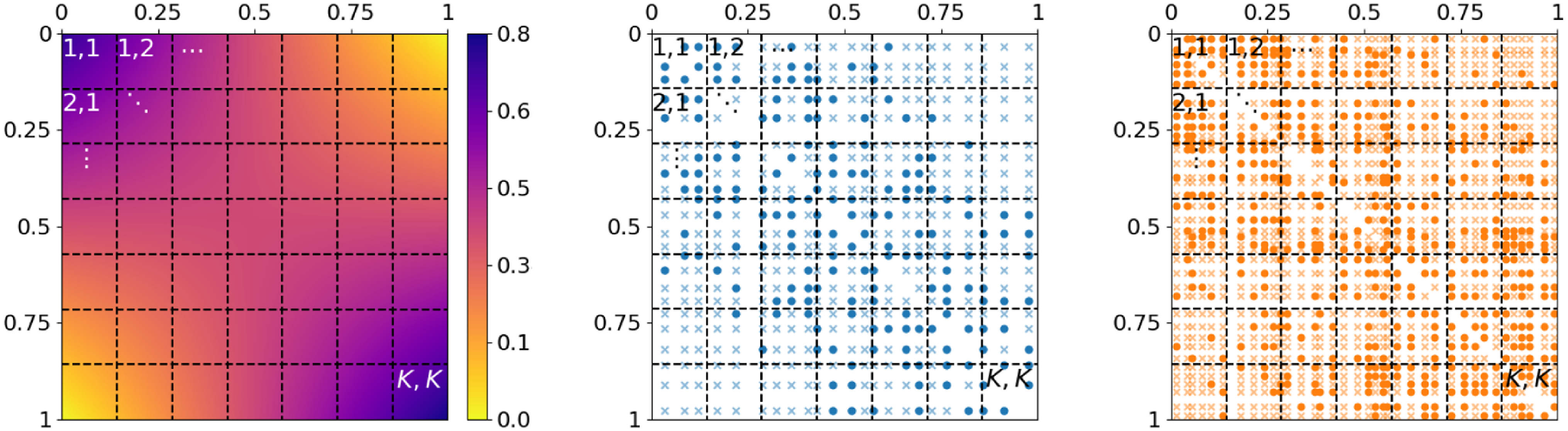
is the Euclidean distance. Following this intuition, we divide the unit square into small segments and compare between networks the ratio of present versus absent edges occurring in these segments (see Figure 2 for an exemplary division). For that purpose, we choose a suitable
$\Vert \cdot \Vert$
is the Euclidean distance. Following this intuition, we divide the unit square into small segments and compare between networks the ratio of present versus absent edges occurring in these segments (see Figure 2 for an exemplary division). For that purpose, we choose a suitable $K \in \mathbb{N}$
, specify a corresponding boundary sequence
$K \in \mathbb{N}$
, specify a corresponding boundary sequence $a_0=0 \lt a_1 \lt \ldots \lt a_K=1$
, and define the following two quantities for
$a_0=0 \lt a_1 \lt \ldots \lt a_K=1$
, and define the following two quantities for $l,k = 1,\ldots ,K$
with
$l,k = 1,\ldots ,K$
with $l \geq k$
:
$l \geq k$
:
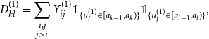
 \begin{align} \begin{split} d_{kl}^{(g)} &= \sum \limits _{\substack {i,j \\ j \gt i}} y_{ij}^{(g)} \unicode {x1D7D9}_{\{u_i^{(g)} \in [a_{k-1}, a_k)\}} \unicode {x1D7D9}_{\{u_j^{(g)} \in [a_{l-1}, a_l)\}} \\ m_{kl}^{(g)} &= \sum \limits _{\substack {i,j \\ j \gt i}} \unicode {x1D7D9}_{\{u_i^{(g)} \in [a_{k-1}, a_k)\}} \unicode {x1D7D9}_{\{u_j^{(g)} \in [a_{l-1}, a_l)\}}. \end{split} \end{align}
This means $d_{kl}^{(g)}$
and
$d_{kl}^{(g)}$
and $m_{kl}^{(g)}$
represent the number of present (
$m_{kl}^{(g)}$
represent the number of present ( $y_{ij}^{(g)} = 1$
) and (a priori) possible edges of network
$y_{ij}^{(g)} = 1$
) and (a priori) possible edges of network $g$
, respectively, within the constructed rectangle
$g$
, respectively, within the constructed rectangle $[a_{k-1}, a_k) \times [a_{l-1}, a_l)$
. The corresponding cross-network counts can be calculated by
$[a_{k-1}, a_k) \times [a_{l-1}, a_l)$
. The corresponding cross-network counts can be calculated by $d_{kl} = d_{kl}^{(1)} + d_{kl}^{(2)}$
and
$d_{kl} = d_{kl}^{(1)} + d_{kl}^{(2)}$
and $m_{kl} = m_{kl}^{(1)} + m_{kl}^{(2)}$
. Note that different network sizes are implicitly taken into account, since the sums in (8) run over the number of edges in network
$m_{kl} = m_{kl}^{(1)} + m_{kl}^{(2)}$
. Note that different network sizes are implicitly taken into account, since the sums in (8) run over the number of edges in network $g$
, which is suppressed in the notation for simplicity of notation. Since
$g$
, which is suppressed in the notation for simplicity of notation. Since $w^{\text{joint}}(\cdot ,\cdot )$
is smooth, we further assume that the induced probability on edge variables within
$w^{\text{joint}}(\cdot ,\cdot )$
is smooth, we further assume that the induced probability on edge variables within $[a_{k-1}, a_k) \times [a_{l-1}, a_l)$
is approximately constant. That allows for putting the observed ratios between present and absent edges in direct relation. In this light, we formulate the following contingency table to keep track of homogeneity between the networks within rectangle
$[a_{k-1}, a_k) \times [a_{l-1}, a_l)$
is approximately constant. That allows for putting the observed ratios between present and absent edges in direct relation. In this light, we formulate the following contingency table to keep track of homogeneity between the networks within rectangle $(k,l)$
:
$(k,l)$
:
Dividing the unit square as domain of the graphon model into small segments for comparing network structure on a microscopic level. Left: division of $w^{\text{joint}}(\cdot ,\cdot )$
into approximately piecewise-constant rectangles. Middle and right: edge positions
$w^{\text{joint}}(\cdot ,\cdot )$
into approximately piecewise-constant rectangles. Middle and right: edge positions $(u_{i}^{(g)}, u_{j}^{(g)})^\top$
of two simulated networks with respect to
$(u_{i}^{(g)}, u_{j}^{(g)})^\top$
of two simulated networks with respect to $w^{\text{joint}}(\cdot ,\cdot )$
; weakly colored crosses and intensively colored circles represent absent and present edges, respectively. The two networks can be compared by pairwise contrasting the edge proportions within the labeled rectangles.
$w^{\text{joint}}(\cdot ,\cdot )$
; weakly colored crosses and intensively colored circles represent absent and present edges, respectively. The two networks can be compared by pairwise contrasting the edge proportions within the labeled rectangles.

Apparently, if $H_0$
is assumed to be true, we would expect the proportions of present edges,
$H_0$
is assumed to be true, we would expect the proportions of present edges, $d_{kl}^{(1)} / m_{kl}^{(1)}$
and
$d_{kl}^{(1)} / m_{kl}^{(1)}$
and $d_{kl}^{(2)} / m_{kl}^{(2)}$
, to be similar. This can be assessed by contrasting the observed numbers of edges with their expectations conditional on the given margin totals, which is in line with the construction of Fisher’s exact test on
$d_{kl}^{(2)} / m_{kl}^{(2)}$
, to be similar. This can be assessed by contrasting the observed numbers of edges with their expectations conditional on the given margin totals, which is in line with the construction of Fisher’s exact test on $2 \times 2$
contingency tables. In this regard, the theoretical random counterpart of
$2 \times 2$
contingency tables. In this regard, the theoretical random counterpart of $d_{kl}^{(1)}$
can be defined as
$d_{kl}^{(1)}$
can be defined as
 \begin{align*} D_{kl}^{(1)} &= \sum \limits _{\substack {i,j \\ j \gt i}} Y_{ij}^{(1)} \unicode {x1D7D9}_{\{u_i^{(1)} \in [a_{k-1}, a_k)\}} \unicode {x1D7D9}_{\{u_j^{(1)} \in [a_{l-1}, a_l)\}}, \end{align*}
for which under $H_0$
it approximately holds that
$H_0$
it approximately holds that
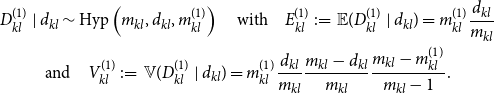 \begin{equation} \begin{gathered} D_{kl}^{(1)} \mid d_{kl} \sim \mbox{Hyp} \left ( m_{kl}, d_{kl}, m_{kl}^{(1)} \right ) \quad \mbox{with} \quad E_{kl}^{(1)} \,:\!=\, \mathbb{E} (D_{kl}^{(1)} \mid d_{kl} ) = m_{kl}^{(1)} \frac {d_{kl}}{m_{kl}} \\ \mbox{and} \quad V_{kl}^{(1)} \,:\!=\, {\mathbb{V}} (D_{kl}^{(1)} \mid d_{kl} ) = m_{kl}^{(1)} \frac {d_{kl}}{m_{kl}} \frac {m_{kl} - d_{kl}}{m_{kl}} \frac {m_{kl} - m_{kl}^{(1)}}{m_{kl} -1}. \end{gathered} \end{equation}
Based on these specifications, we define our test statistic as
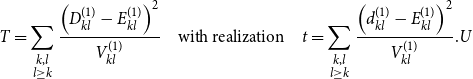 \begin{equation} T = \sum \limits _{\substack {k,l \\ l \geq k}} \frac {\left ( D_{kl}^{(1)} - E_{kl}^{(1)} \right )^2}{ V_{kl}^{(1)} } \quad \mbox{with realization} \quad t = \sum \limits _{\substack {k,l \\ l \geq k}} \frac {\left ( d_{kl}^{(1)} - E_{kl}^{(1)} \right )^2}{ V_{kl}^{(1)} }.U \end{equation}
Note that here we only sum over the squared standardized deviations of the first network as the hypergeometric distribution is symmetric, making the same information for the second network redundant. Moreover, summands for which $V_{kl}^{(1)} = 0$
—resulting from
$V_{kl}^{(1)} = 0$
—resulting from $m_{kl}^{(1)}$
,
$m_{kl}^{(1)}$
, $m_{kl} - m_{kl}^{(1)}$
,
$m_{kl} - m_{kl}^{(1)}$
, $d_{kl}$
, or
$d_{kl}$
, or $m_{kl} - d_{kl}$
being zero—carry no relevant information and thus can simply be omitted from the calculation. We can now easily simulate a sample of the distribution under
$m_{kl} - d_{kl}$
being zero—carry no relevant information and thus can simply be omitted from the calculation. We can now easily simulate a sample of the distribution under $H_0$
by drawing
$H_0$
by drawing $D_{kl}^{(1)} \mid d_{kl}$
according to (9) and calculating
$D_{kl}^{(1)} \mid d_{kl}$
according to (9) and calculating $T$
as in (10). From this, we can easily derive a critical value
$T$
as in (10). From this, we can easily derive a critical value $c_{1-\alpha }$
or
$c_{1-\alpha }$
or $p$
-value by comparing the realization
$p$
-value by comparing the realization $t$
of the simulated values. Moreover, asymptotic calculation is possible if
$t$
of the simulated values. Moreover, asymptotic calculation is possible if $m_{kl}^{(1)}$
is large,
$m_{kl}^{(1)}$
is large, $m_{kl}$
and
$m_{kl}$
and $d_{kl}$
are large compared to
$d_{kl}$
are large compared to $m_{kl}^{(1)}$
, and
$m_{kl}^{(1)}$
, and $d_{kl} / m_{kl}$
is not close to zero or one. Then
$d_{kl} / m_{kl}$
is not close to zero or one. Then $D_{kl}^{(1)}$
is approximately normally distributed and we can conclude that
$D_{kl}^{(1)}$
is approximately normally distributed and we can conclude that
 \begin{equation} T \stackrel {\text{a}}{\sim } \chi ^2_{K (K+1) / 2}. \end{equation}
Here, the test statistic is essentially the sum of squared (conditionally) independent random variables that approximately follow a standard normal distribution. This allows again to derive a critical value or a $p$
-value, respectively. The choice of an appropriate
$p$
-value, respectively. The choice of an appropriate $K$
applied for these calculations is discussed in Section C of the Appendix. Note that altogether the presented test procedure follows a conception similar to the one underlying the log-rank test for time-to-event data, which also includes the construction of a conditional distribution as in (9). Regarding the latter, it seems worth noting that conditioning on the margins in the corresponding contingency table does not imply adding any assumptions on
$K$
applied for these calculations is discussed in Section C of the Appendix. Note that altogether the presented test procedure follows a conception similar to the one underlying the log-rank test for time-to-event data, which also includes the construction of a conditional distribution as in (9). Regarding the latter, it seems worth noting that conditioning on the margins in the corresponding contingency table does not imply adding any assumptions on $w^{(1)}(\cdot , \cdot )$
or
$w^{(1)}(\cdot , \cdot )$
or $w^{(2)}(\cdot , \cdot )$
, or the structural relation between these two. It rather means to presume that the realization of these marginal totals carries no information about the relationship between
$w^{(2)}(\cdot , \cdot )$
, or the structural relation between these two. It rather means to presume that the realization of these marginal totals carries no information about the relationship between $w^{(1)}(\cdot , \cdot )$
and
$w^{(1)}(\cdot , \cdot )$
and $w^{(2)}(\cdot , \cdot )$
, equivalently as for Fisher’s test on contingency tables (Yates Reference Yates1984). We also refer to (Lang Reference Lang1996) for further discussion in this line.
$w^{(2)}(\cdot , \cdot )$
, equivalently as for Fisher’s test on contingency tables (Yates Reference Yates1984). We also refer to (Lang Reference Lang1996) for further discussion in this line.
Apparently, when conducting the test procedure on real-world networks, we obtain the joint graphon and the corresponding alignment of the networks by applying the estimation procedure described in Section 4. In the end, this enables us to appropriately approximate test statistic (10). In this context, it is important to consider the general behavior of the joint graphon estimation under the alternative, that is, if hypothesis (4) does not hold. We stress that the intuition of the estimation procedure is to align the two networks as well as possible with respect to some suitable joint graphon model. Consequently, the expectation of $T$
will be higher the more the true graphons
$T$
will be higher the more the true graphons $w^{(1)}(\cdot ,\cdot )$
and
$w^{(1)}(\cdot ,\cdot )$
and $w^{(2)}(\cdot ,\cdot )$
differ after “optimal” alignment. This clearly implies that the power of our test is higher for instances that deviate more strongly from the null hypothesis.
$w^{(2)}(\cdot ,\cdot )$
differ after “optimal” alignment. This clearly implies that the power of our test is higher for instances that deviate more strongly from the null hypothesis.
6. Applications
In this section, we showcase the applicability of the joint graphon estimation routine and the subsequent testing procedure. To give a comprehensive insight, this comprises both simulated and real-world networks. For an optimal estimation result and to best approximate test statistic (10), we repeat the estimation and testing procedure several times. In a modeling-oriented context, we would then typically pick the outcome with the lowest corrected $\operatorname {AIC}$
. However, since here the focus is on the statistical testing aspect, we choose the estimation result which leads to the highest
$\operatorname {AIC}$
. However, since here the focus is on the statistical testing aspect, we choose the estimation result which leads to the highest $p$
-value, assuming that this provides an optimal lower bound for the outcome under the (potentially existing) oracle network alignment.
$p$
-value, assuming that this provides an optimal lower bound for the outcome under the (potentially existing) oracle network alignment.
Moreover, applying test statistic (10) requires to specify $K$
and the sequence
$K$
and the sequence $a_0, \ldots , a_K$
. For the sake of simplicity and due to its minor impact, in the following applications we employ equidistant boundaries
$a_0, \ldots , a_K$
. For the sake of simplicity and due to its minor impact, in the following applications we employ equidistant boundaries $a_0, \ldots , a_K$
as an intuitive approach, that is, setting
$a_0, \ldots , a_K$
as an intuitive approach, that is, setting $a_k = k/K$
. In turn, under equidistant node positions, the consistent number of network entries per network and rectangle,
$a_k = k/K$
. In turn, under equidistant node positions, the consistent number of network entries per network and rectangle, $m_{kl}^{(g)}$
, can be easily deduced, and we choose
$m_{kl}^{(g)}$
, can be easily deduced, and we choose $K$
such that this parameter is “not too small” for both networks. For more details, see Section C of the Appendix.
$K$
such that this parameter is “not too small” for both networks. For more details, see Section C of the Appendix.
6.1 Simulation studies
6.1.1 Exemplary application to synthetic data
Joint graphon estimation for simulated networks with subsequent testing on equivalence of the underlying distribution models. The top row shows the true and the jointly estimated graphon on the left and right, respectively. The realizations of the terms of test statistic (10), representing the dissimilarities of the two networks per rectangle, are visualized at the bottom left, where $m_{kl}^{(g)} \geq 100$
for
$m_{kl}^{(g)} \geq 100$
for $k \neq l$
and
$k \neq l$
and $\geq 45$
otherwise (cf. contingency table on page 16). The final result of the test statistic (black solid vertical line) as well as its distribution under
$\geq 45$
otherwise (cf. contingency table on page 16). The final result of the test statistic (black solid vertical line) as well as its distribution under $H_0$
are illustrated at the bottom right, where the black solid step function and the blue dashed curve depict the simulated and the asymptotic chi-squared distribution, respectively. The red dashed vertical lines (separated by red dot) visualize the critical values at a significance level of
$H_0$
are illustrated at the bottom right, where the black solid step function and the blue dashed curve depict the simulated and the asymptotic chi-squared distribution, respectively. The red dashed vertical lines (separated by red dot) visualize the critical values at a significance level of $5\%$
, derived from the simulated (upper line) and the asymptotic distribution (lower line).
$5\%$
, derived from the simulated (upper line) and the asymptotic distribution (lower line).
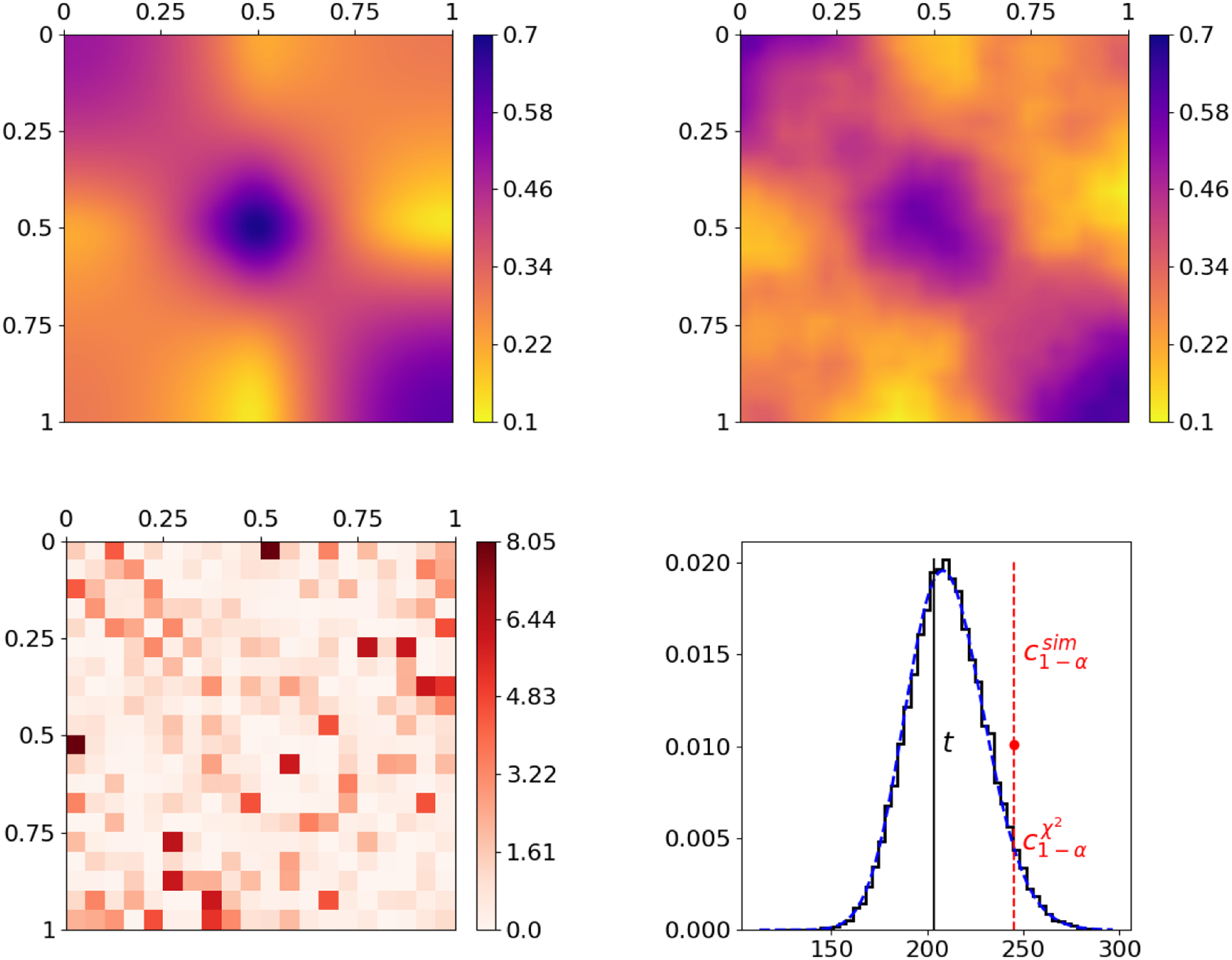
To demonstrate the general capability of the joint graphon estimation and the performance of the subsequent testing procedure, we consider the graphon in the top left plot of Figure 3. Its formation is inspired by and can be interpreted as a stochastic blockmodel with smooth transitions between communities. Based on this ground-truth model specification, we simulate two networks with $N^{(1)} = 200$
and
$N^{(1)} = 200$
and $N^{(2)} = 300$
by making use of data-generating process (2). The underlying structure can then be recovered by applying the joint graphon estimation, where, for initialization, we make use of an uninformative random node positioning. This yields the graphon estimate at the top right, which apparently fully captures the structure of the ground-truth graphon. Based on the associated estimated node positions, we subsequently conduct the testing procedure on whether the underlying distributions are equivalent. To this end, we start with calculating the rectangle-wise differences according to the construction of test statistic (10). The results are depicted as a heat map at the bottom left plot of Figure 3. This reveals that the difference in the local edge density is rather low to moderate in most rectangles, whereas it is distinctly higher in a few others. Aggregating these differences yields a test statistic of
$N^{(2)} = 300$
by making use of data-generating process (2). The underlying structure can then be recovered by applying the joint graphon estimation, where, for initialization, we make use of an uninformative random node positioning. This yields the graphon estimate at the top right, which apparently fully captures the structure of the ground-truth graphon. Based on the associated estimated node positions, we subsequently conduct the testing procedure on whether the underlying distributions are equivalent. To this end, we start with calculating the rectangle-wise differences according to the construction of test statistic (10). The results are depicted as a heat map at the bottom left plot of Figure 3. This reveals that the difference in the local edge density is rather low to moderate in most rectangles, whereas it is distinctly higher in a few others. Aggregating these differences yields a test statistic of $203.2$
as depicted by the black solid vertical line at the bottom right. Contrasting this result with the simulated
$203.2$
as depicted by the black solid vertical line at the bottom right. Contrasting this result with the simulated $95\%$
quantile of the distribution of
$95\%$
quantile of the distribution of $T$
under
$T$
under $H_0$
as the critical value (red dashed vertical line) yields no rejection. Hence, the underlying distributions of the two networks do not significantly differ with respect to a significance level of
$H_0$
as the critical value (red dashed vertical line) yields no rejection. Hence, the underlying distributions of the two networks do not significantly differ with respect to a significance level of $5\%$
. As a final remark with regard to the bottom right plot, the simulated distribution of
$5\%$
. As a final remark with regard to the bottom right plot, the simulated distribution of $T$
(black solid step function) and its theoretical approximation (blue dashed curve)—both relying on the assumption of
$T$
(black solid step function) and its theoretical approximation (blue dashed curve)—both relying on the assumption of $H_0$
being true—are very close to one another. Consequently, they also provide very similar critical values, namely
$H_0$
being true—are very close to one another. Consequently, they also provide very similar critical values, namely $243.6$
and
$243.6$
and $244.8$
, respectively. This demonstrates that asymptotic distribution (11) represents a good approximation.
$244.8$
, respectively. This demonstrates that asymptotic distribution (11) represents a good approximation.
6.1.2 Performance analysis under $H_0$
$H_0$

To evaluate the performance of the testing procedure in this example more profoundly, we repeat the above proceeding $400$
times, with newly simulated networks in each trial (remaining with
$400$
times, with newly simulated networks in each trial (remaining with $N^{(1)} = 200$
and
$N^{(1)} = 200$
and $N^{(2)} = 300$
). Note that we run the estimation procedure always ten times (with different random node positions as varying initialization) and finally pick the highest
$N^{(2)} = 300$
). Note that we run the estimation procedure always ten times (with different random node positions as varying initialization) and finally pick the highest $p$
-value as the actual result for the given network pair. These repetitions already provide a broad insight into the method’s performance under the given setting. An even more extensive evaluation becomes possible when, in contrast to the proceeding above, the testing procedure is performed on the basis of the oracle node positions. These positions already describe an optimal network alignment and can thus be used directly as a substitute for
$p$
-value as the actual result for the given network pair. These repetitions already provide a broad insight into the method’s performance under the given setting. An even more extensive evaluation becomes possible when, in contrast to the proceeding above, the testing procedure is performed on the basis of the oracle node positions. These positions already describe an optimal network alignment and can thus be used directly as a substitute for $(\hat {{\boldsymbol{u}}}^{(1)},\hat {{\boldsymbol{u}}}^{(2)})$
that will even lead to the smallest test statistic possible. Moreover, it allows us to dramatically reduce the computational burden since it releases us from the preceding (computationally expensive) model estimation. As a consequence, we are able to increase the number of conducted tests to
$(\hat {{\boldsymbol{u}}}^{(1)},\hat {{\boldsymbol{u}}}^{(2)})$
that will even lead to the smallest test statistic possible. Moreover, it allows us to dramatically reduce the computational burden since it releases us from the preceding (computationally expensive) model estimation. As a consequence, we are able to increase the number of conducted tests to $10,000$
. From these two repetition studies (using either
$10,000$
. From these two repetition studies (using either $\hat {{\boldsymbol{u}}}^{(g)}$
or
$\hat {{\boldsymbol{u}}}^{(g)}$
or ${\boldsymbol{u}}^{(g)}$
), we obtain rejection rates of
${\boldsymbol{u}}^{(g)}$
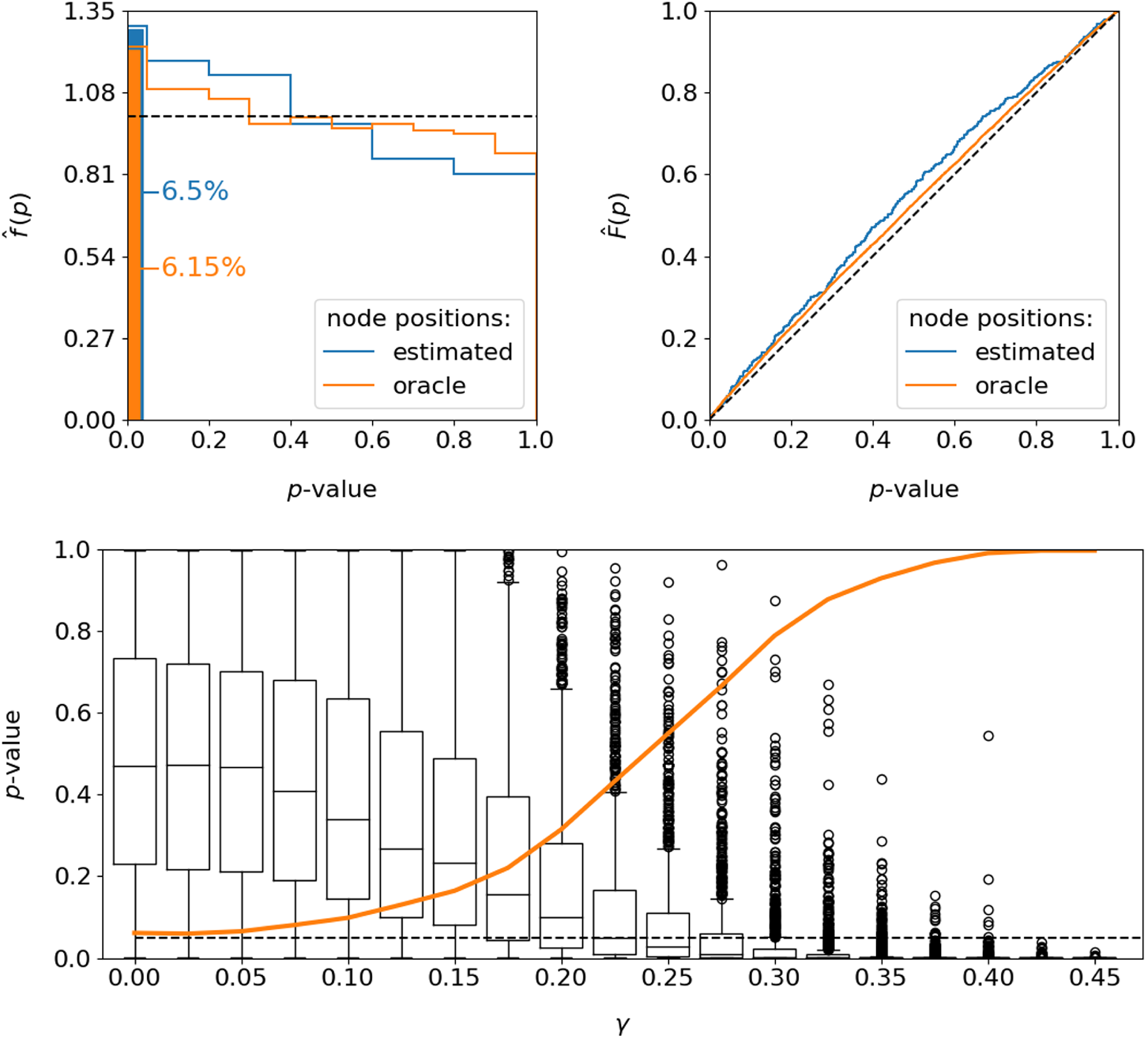
), we obtain rejection rates of $6.5\%$
and
$6.5\%$
and $6.15\%$
under the estimated and oracle node positioning, respectively. That means the test is slightly overconfident relative to the nominal significance level of
$6.15\%$
under the estimated and oracle node positioning, respectively. That means the test is slightly overconfident relative to the nominal significance level of $5\%$
. The test is not exact in any way, as it is built upon the asymptotic statement (11) which explains the small bias of the test. The top row of Figure 4 shows additionally the empirical distributions of the observed
$5\%$
. The test is not exact in any way, as it is built upon the asymptotic statement (11) which explains the small bias of the test. The top row of Figure 4 shows additionally the empirical distributions of the observed $p$
-values, illustrated as densities (left) and cumulative distribution functions (right). In accordance with the mildly inflated rejection rates, this exhibits a slight tendency to underestimate the
$p$
-values, illustrated as densities (left) and cumulative distribution functions (right). In accordance with the mildly inflated rejection rates, this exhibits a slight tendency to underestimate the $p$
-value, i.e. interpreting the discrepancy as too high in distributional terms.
$p$
-value, i.e. interpreting the discrepancy as too high in distributional terms.
Performance of the testing procedure with regard to the resulting $p$
-value; results are simulation-based. Top: empirical distribution of the
$p$
-value; results are simulation-based. Top: empirical distribution of the $p$
-value under
$p$
-value under $H_0$
, illustrated as density (left, including a depiction of rejection rates at significance level of 5%) and cumulative distribution function (right). The black dashed lines illustrate the desired distributional behavior of an optimal test. Number of repetitions for estimated / oracle node positions:
$H_0$
, illustrated as density (left, including a depiction of rejection rates at significance level of 5%) and cumulative distribution function (right). The black dashed lines illustrate the desired distributional behavior of an optimal test. Number of repetitions for estimated / oracle node positions: $400$
/
$400$
/ $10,000$
. Bottom: distribution of the
$10,000$
. Bottom: distribution of the $p$
-value under
$p$
-value under $H_1$
and the usage of oracle node positions (in box plot format); based on
$H_1$
and the usage of oracle node positions (in box plot format); based on $1,000$
repetitions each. The x-axis illustrates different settings according to formulation (12) (higher value of
$1,000$
repetitions each. The x-axis illustrates different settings according to formulation (12) (higher value of $\gamma$
implies stronger deviation from
$\gamma$
implies stronger deviation from $H_0$
). The black dashed horizontal line represents the
$H_0$
). The black dashed horizontal line represents the $5\%$
significance level, and the orange curve illustrates the corresponding power.
$5\%$
significance level, and the orange curve illustrates the corresponding power.
6.1.3 Performance analysis under
$H_1$

Conclusively, we are interested in evaluating the test performance under a false null hypothesis, which apparently requires formulating a suitable alternative. To this end, we “shrink” the heterogeneity within the graphon such that the present structure becomes less pronounced. The resulting graphon specification consequently tends more towards an Erdős–Rényi model, with the global density remaining unchanged. To be precise, based on $w^{(1)}(\cdot ,\cdot )$
, we formulate
$w^{(1)}(\cdot ,\cdot )$
, we formulate
 \begin{align} w^{(2)}(u, v) \,:\!=\, (1 - \gamma ) \, w^{(1)}(u,v) + \gamma \, \bar {w}^{(1)} \end{align}
with $\gamma \in [0,1]$
and
$\gamma \in [0,1]$
and $\bar {w}^{(1)} = \iint w^{(1)}(u,v) \mathop {}\!\mathrm{d} u \mathop {}\!\mathrm{d} v$
. Apparently, increasing the mixing parameter
$\bar {w}^{(1)} = \iint w^{(1)}(u,v) \mathop {}\!\mathrm{d} u \mathop {}\!\mathrm{d} v$
. Apparently, increasing the mixing parameter $\gamma$
leads to a stronger deviation from
$\gamma$
leads to a stronger deviation from $H_0$
. At the same time, this setting guarantees an optimal alignment of
$H_0$
. At the same time, this setting guarantees an optimal alignment of $w^{(1)}(\cdot ,\cdot )$
and
$w^{(1)}(\cdot ,\cdot )$
and $w^{(2)}(\cdot ,\cdot )$
, meaning that there exists no rearrangement of
$w^{(2)}(\cdot ,\cdot )$
, meaning that there exists no rearrangement of $w^{(2)}(\cdot ,\cdot )$
that is closer to
$w^{(2)}(\cdot ,\cdot )$
that is closer to $w^{(1)}(\cdot ,\cdot )$
than specification (12). For this experiment, we again choose
$w^{(1)}(\cdot ,\cdot )$
than specification (12). For this experiment, we again choose $N^{(1)} = 200$
and
$N^{(1)} = 200$
and $N^{(2)} = 300$
. Moreover, here we rely exclusively on the oracle node positions. This provides a lower bound of the power since the rejection rate can be expected to be higher when using estimated node positions instead (cf. previous analysis under
$N^{(2)} = 300$
. Moreover, here we rely exclusively on the oracle node positions. This provides a lower bound of the power since the rejection rate can be expected to be higher when using estimated node positions instead (cf. previous analysis under $H_0$
). The results for this setup are presented in the bottom plot of Figure 4, where the distribution of the resulting
$H_0$
). The results for this setup are presented in the bottom plot of Figure 4, where the distribution of the resulting $p$
-value is illustrated for different settings of
$p$
-value is illustrated for different settings of $\gamma$
. The orange curve additionally visualizes the resulting power, i.e. the proportion of cases with
$\gamma$
. The orange curve additionally visualizes the resulting power, i.e. the proportion of cases with $p \lt 0.05$
. These results clearly show that the probability of detecting the false null hypothesis monotonically increases as the parameter
$p \lt 0.05$
. These results clearly show that the probability of detecting the false null hypothesis monotonically increases as the parameter $\gamma$
gets larger, which underpins the appropriateness of our test procedure.
$\gamma$
gets larger, which underpins the appropriateness of our test procedure.
Overall, the obtained simulation results demonstrate that the elaborated estimation and testing procedure yields reasonable results for assessing structural differences between networks. Building upon these findings, we next want to investigate the method’s performance on real-world data.
6.2 Real-world examples
6.2.1 Facebook ego networks
As a first real-world example, we consider two Facebook ego networks, with each describing the friendship behavior between all friends of one user (“ego”). These networks have been assembled by Leskovec and McAuley (Reference Leskovec and McAuley2012) and are publicly available on the Stanford Large Network Dataset Collection (Leskovec and Krevl, Reference Leskovec and Krevl2014). The two ego networks consist of $333$
and
$333$
and $168$
individuals, respectively, where the ego nodes are not included. An illustration of these networks is given in the top row of Figure 5, with nodes being colored according to resulting positions. In both networks, these final estimated node positions appear to be in line with the given network structure in terms of reflecting the nodes’ embedding within the network. Moreover, they seem to be aligned across networks. For example, in both networks, the reddish nodes represent the rather centric individuals, whereas the nodes from the dark blue spectrum constitute a moderately interconnected branch that is more detached from the rest of the network. However, the segment-wise differences depicted at the bottom left in Figure 5 exhibit some strong deviations. This can be clearly traced back to the blockwise division of the adjacency matrices as it results from partitioning the domain of edge positions (middle row). The aggregated differences ultimately result in a test statistic that is far from the sector of plausible values under the null hypothesis, as illustrated at the bottom right. Consequently, we can conclude that the structural behavior in the two networks differs significantly.
$168$
individuals, respectively, where the ego nodes are not included. An illustration of these networks is given in the top row of Figure 5, with nodes being colored according to resulting positions. In both networks, these final estimated node positions appear to be in line with the given network structure in terms of reflecting the nodes’ embedding within the network. Moreover, they seem to be aligned across networks. For example, in both networks, the reddish nodes represent the rather centric individuals, whereas the nodes from the dark blue spectrum constitute a moderately interconnected branch that is more detached from the rest of the network. However, the segment-wise differences depicted at the bottom left in Figure 5 exhibit some strong deviations. This can be clearly traced back to the blockwise division of the adjacency matrices as it results from partitioning the domain of edge positions (middle row). The aggregated differences ultimately result in a test statistic that is far from the sector of plausible values under the null hypothesis, as illustrated at the bottom right. Consequently, we can conclude that the structural behavior in the two networks differs significantly.
Comparison of two facebook ego networks. Top: illustration of networks with coloring referring to estimated node positions. Middle: ordered adjacency matrices divided into blockwise segments. Bottom left: segment-wise differences between the two networks with $m_{kl}^{(g)} \geq 100$
for
$m_{kl}^{(g)} \geq 100$
for $k \neq l$
and
$k \neq l$
and $\geq 45$
otherwise (cf. contingency table on page 16); gray rectangles do not contain any observed edges (
$\geq 45$
otherwise (cf. contingency table on page 16); gray rectangles do not contain any observed edges ( $d_{kl}=0$
) and thus provide no information. Bottom right: realization of test statistic (black solid vertical line) plus corresponding distribution under
$d_{kl}=0$
) and thus provide no information. Bottom right: realization of test statistic (black solid vertical line) plus corresponding distribution under $H_0$
(black solid step function and blue dashed curve represent simulated and asymptotic chi-squared distribution, respectively); critical values derived from the two types of distributions are represented by the upper and the lower red dashed vertical line (separated by red dot).
$H_0$
(black solid step function and blue dashed curve represent simulated and asymptotic chi-squared distribution, respectively); critical values derived from the two types of distributions are represented by the upper and the lower red dashed vertical line (separated by red dot).
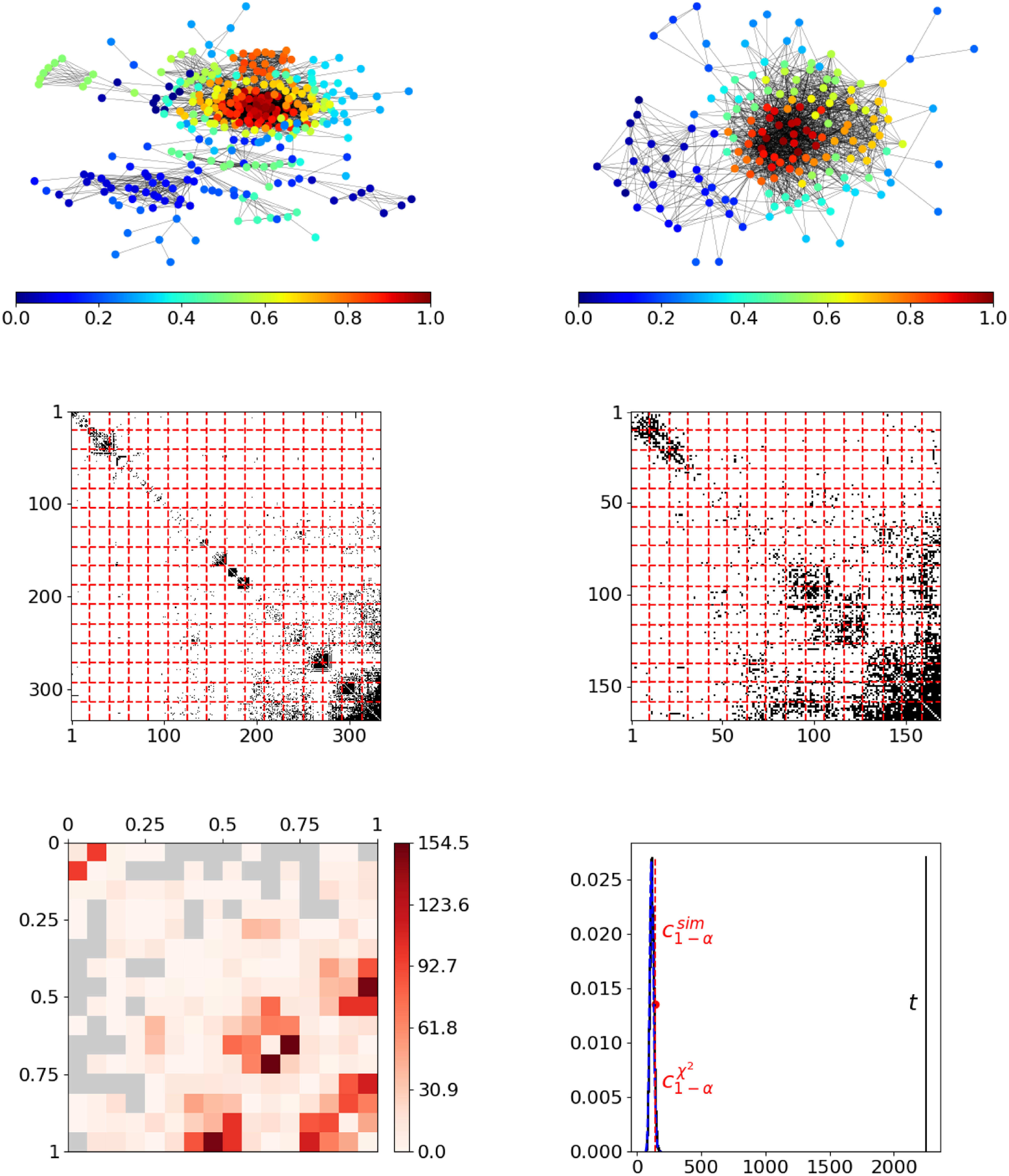
6.2.2 Human brain functional coactivation networks
In the second real-world application, we are concerned with differences in the human brain coactivation structure. To be precise, we compare two types of individuals, one with autism spectrum disorder (ASD) and the other with typical development (TD). In particular, we are interested in whether the functional connectivity within the brain significantly differs between these two groups (cf. the introductory example from Figure 1). For this analysis, we use resting-state functional magnetic resonance imaging data from the Autism Brain Imaging Data Exchange project (ABIDE I, Reference Abide2013). More specifically, we employ preprocessed data provided by the Preprocessed Connectomes Project platform (PCP 2015). Based on these person-specific datasets, we first calculate correlations between brain regions with respect to concurrent activation over time. Aggregating the results of participants from the same clinical group and employing an appropriate threshold finally yields the network-structured data which we aim to compare. To be precise, by performing the described preprocessing, we achieve for both groups, ASD and TD, a global connectivity pattern between $116$
prespecified relevant brain regions. Note that these regions are the same for both groups, which is why this could also be viewed as a comparison task under known node correspondence. However, we emphasize that in neurosciences, the transfer of competencies between brain regions is a well-known phenomenon, wherefore the general functional connectivity structure might be of greater relevance than the functional connection between specific regions. Further details on the acquisition and adequate transformation of the data are provided in Section D of the Appendix.
$116$
prespecified relevant brain regions. Note that these regions are the same for both groups, which is why this could also be viewed as a comparison task under known node correspondence. However, we emphasize that in neurosciences, the transfer of competencies between brain regions is a well-known phenomenon, wherefore the general functional connectivity structure might be of greater relevance than the functional connection between specific regions. Further details on the acquisition and adequate transformation of the data are provided in Section D of the Appendix.
Comparison of functional coactivation in the human brain between groups of subjects with autism spectrum disorder and with typical development. The top row shows the networks of the ASD and the TD group on the left- and right-hand side, respectively. All illustration aspects are equivalent to the representation in Figure 5. The number of nodes per rectangle is again given by $m_{kl}^{(g)} \geq 100$
for
$m_{kl}^{(g)} \geq 100$
for $k \neq l$
and
$k \neq l$
and $\geq 45$
otherwise, where N/A’s in the blockwise differences result from
$\geq 45$
otherwise, where N/A’s in the blockwise differences result from $d_{kl}$
or
$d_{kl}$
or $m_{kl} - d_{kl}$
being zero.
$m_{kl} - d_{kl}$
being zero.
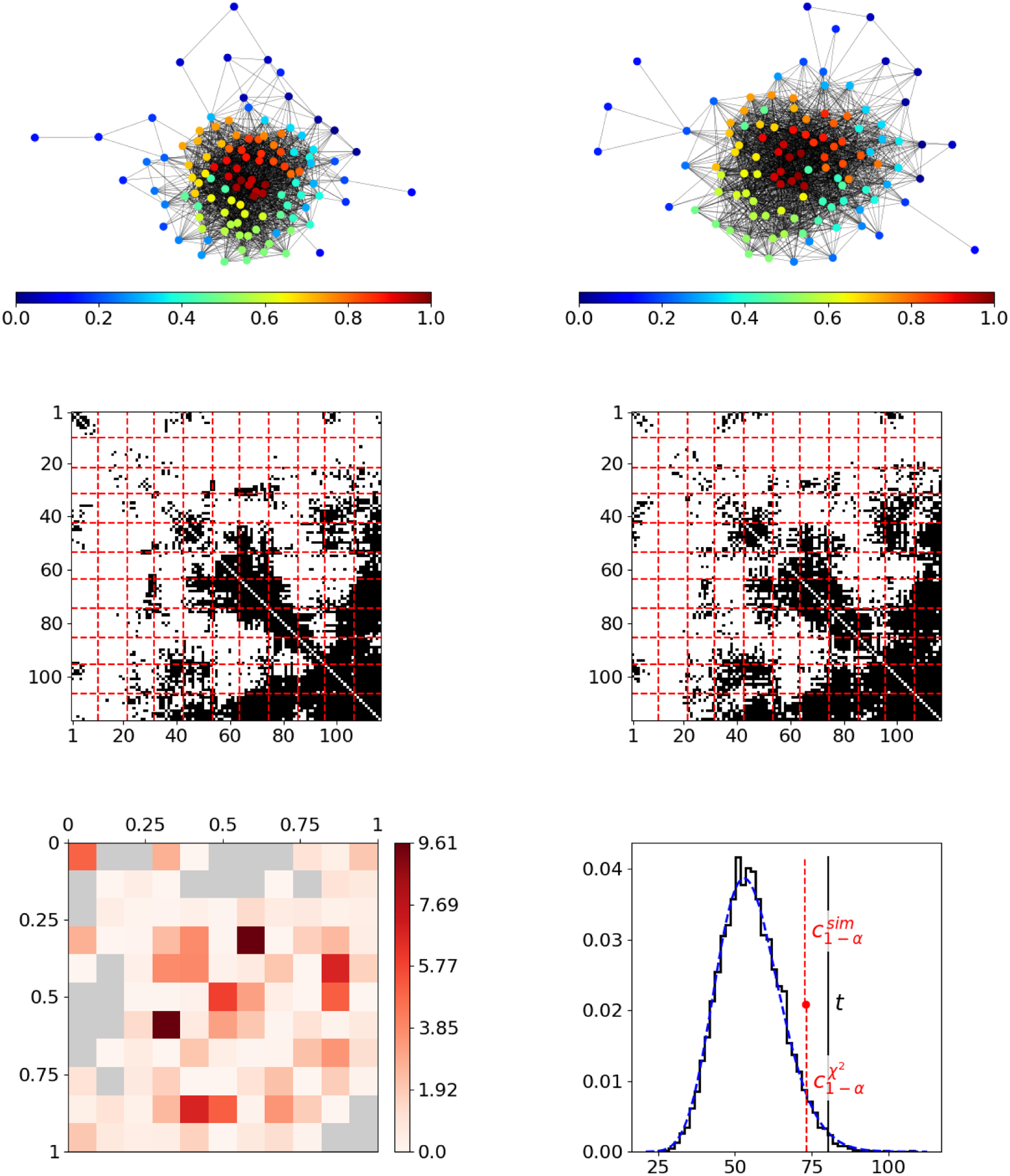
For analyzing the differences in the brain coactivation structure between the two diagnostic groups, we again start with appropriately aligning the two networks. This is apparently done by employing the joint graphon estimation routine. The resulting node positions in relation to the embedding of nodes within the networks are illustrated in the top row of Figure 6. Again this reveals a plausible allocation of the nodes in the joint graphon model. The structural evolvement can further be evaluated by consulting the correspondingly ordered adjacency matrices (see middle row), where the red dashed lines represent the blockwise division resulting from the assignment of the edge positions to the rectangles in $[0,1]$
. At first view, the formed structure looks quite similar in both matrices. Yet, on closer inspection, some blocks can be found where the density seems considerably different. This is also observed in the rectangle-wise differences depicted in the bottom left plot. In the end, aggregating these differences leads to a
$[0,1]$
. At first view, the formed structure looks quite similar in both matrices. Yet, on closer inspection, some blocks can be found where the density seems considerably different. This is also observed in the rectangle-wise differences depicted in the bottom left plot. In the end, aggregating these differences leads to a $p$
-value of
$p$
-value of $0.013$
which gives a strong indication against the null hypothesis.
$0.013$
which gives a strong indication against the null hypothesis.
Given that this outcome does not support an utterly unambiguous decision of the conducted test procedure, one might additionally be interested in the nature of the inferred differences. To address this, in Section 1.2 of the Supplementary Material, we localize different behavior between the networks on the microscopic scale. Note that this can also be derived more or less directly from the joint graphon model. Moreover, for comparison reasons, we repeated the above analysis for two randomly selected disjoint subgroups of the TD group. According to the results illustrated in Figure 6 of the Supplementary Material, in this scenario, we do not observe a significant overall deviation. This further underlines the findings about the dissimilarity between the ASD and the TD group.
7. Discussion and conclusion
In the literature on network comparison, the task of drawing statistical inference appears to be an open challenge up to now. In this paper, we addressed this shortcoming by developing a nonparametric test on the equivalence of network structures. As a basis, we utilized joint smooth graphon estimation in order to arrange the networks in a meaningful way. In turn, this allowed us to compare the networks’ densities at a local level. Appropriately quantifying and aggregating the differences between these densities finally enabled us to construct a nonparametric testing procedure on structural equivalence of networks. Given that graphons induce dense networks, our approach is restricted to such networks and an extension to sparse networks is questionable.
The proposed strategy of ordering networks in common relation is very similar to what is often referred to in the literature as “network alignment” (Kuchaiev et al., Reference Kuchaiev, Milenković, Memišević, Hayes and Pržulj2010). However, as an essential distinction to classical network alignment strategies, our method does not seek to find a node-wise one-to-one mapping. Instead, it implies a mapping of local components, meaning small fuzzy groups of nodes with similar structural roles in their respective domains.
Specifically, this also allows the networks to be of different sizes. In fact, the graphon model’s property of decoupling structure and size is crucial for the proposed approach to work. In the same line, one could think of further decoupling the global density by following the approach of Bickel and Chen (Reference Bickel and Chen2009), i.e. by introducing network-related quantities $\rho ^{(g)}$
that serve as individual density coefficients. Specifically, this means modifying formulation (2) by employing
$\rho ^{(g)}$
that serve as individual density coefficients. Specifically, this means modifying formulation (2) by employing $\rho ^{(g)} w^{(g)}(\cdot , \cdot )$
, where
$\rho ^{(g)} w^{(g)}(\cdot , \cdot )$
, where $\hat {\rho }^{(g)}= [N^{(g)} (N^{(g)} -1)]^{-1} \sum _{i,j} y_{ij}^{(g)}$
could serve as an estimate that is independent of the rest of the structure. Such a framework consequentially might lead to a more balanced comparison strategy.
$\hat {\rho }^{(g)}= [N^{(g)} (N^{(g)} -1)]^{-1} \sum _{i,j} y_{ij}^{(g)}$
could serve as an estimate that is independent of the rest of the structure. Such a framework consequentially might lead to a more balanced comparison strategy.
Beyond the applications presented in the previous section, which all refer to the situation with two networks, the method could easily be extended to cases with multiple or even a single network. For example, in the one-sample setting, to test whether a given network follows a hypothetical distribution $\mathbb{P} (\boldsymbol{Y} = \cdot \, ; \, w(\cdot , \cdot ) , N )$
, we could first align the network with the theoretical graphon. That is, applying the E-step based on
$\mathbb{P} (\boldsymbol{Y} = \cdot \, ; \, w(\cdot , \cdot ) , N )$
, we could first align the network with the theoretical graphon. That is, applying the E-step based on $w(\cdot , \cdot )$
. Given this alignment, we could then turn distributional assumption (9) into a binomial distribution with the rectangle-specific mean over
$w(\cdot , \cdot )$
. Given this alignment, we could then turn distributional assumption (9) into a binomial distribution with the rectangle-specific mean over $w(\cdot , \cdot )$
as success probability, and, based on that, calculate the test statistic as in (10).
$w(\cdot , \cdot )$
as success probability, and, based on that, calculate the test statistic as in (10).
Besides the testing aspect, our approach could further be used to uncover relevant differences between networks on the microscopic scale. To be precise, determining the nodes or edges (present or absent) that contribute most to a quantified structural discrepancy between networks is possibly interesting in many situations. This is further elaborated in Section 1.1 of the Supplementary Material.
As a last application case, the joint graphon estimation could further be used to predict edges between separated networks by considering the cross-sample probabilities $w^{\text{joint}}(u_{i_1}^{(1)} , u_{i_2}^{(2)})$
. This might be of interest when two (or more) networks are assumed to be samples of a larger global network. To the best of our knowledge, this has not been pursued by any other approach so far and hence constitutes a novel perspective. As a particular hurdle in this framework, the sampling strategy that is supposed for the drawing of subnetworks needs to be taken into account in the estimation routine. As far as this is not the simple Induced Subgraph Sampling, where one selects a simple random sample of nodes within which all edges are observed, further adaptations are required. Hence, this lies beyond the scope of the paper.
$w^{\text{joint}}(u_{i_1}^{(1)} , u_{i_2}^{(2)})$
. This might be of interest when two (or more) networks are assumed to be samples of a larger global network. To the best of our knowledge, this has not been pursued by any other approach so far and hence constitutes a novel perspective. As a particular hurdle in this framework, the sampling strategy that is supposed for the drawing of subnetworks needs to be taken into account in the estimation routine. As far as this is not the simple Induced Subgraph Sampling, where one selects a simple random sample of nodes within which all edges are observed, further adaptations are required. Hence, this lies beyond the scope of the paper.
Supplementary material
-
(i) Description for deriving differences between networks at the microscopic level. As exemplary application, the two brain networks from Section 6.2.2 are considered.
-
(ii) Replication of the test on functional coactivation networks for two subgroups of the typical-development group (confer Section 6.2.2).
-
(iii) Python-package containing the code to perform the comparison methods described in the paper. The package also contains the preprocessed data of the human brain functional coactivation networks (see Section 6.2.2). (GNU zipped tar file).
Competing interests.
None.
Data availability statement.
All data used in the paper are publicly available. References are given in the paper.
Funding statement.
This work was partially funded by the BERD@NFDI Consortium ( https://www.berd-nfdi.de ).
Appendix
A. Implementation of the Gibbs sampler
In an iterative joint graphon estimation procedure, the joint posterior distribution of the node positions given $w^{\text{joint}}(\cdot ,\cdot )$
and the networks
$w^{\text{joint}}(\cdot ,\cdot )$
and the networks $\boldsymbol{y}^{(1)}$
and
$\boldsymbol{y}^{(1)}$
and $\boldsymbol{y}^{(2)}$
can be simulated by constructing a Gibbs sampler. We stress that the node positions are independent between networks and thus the Gibbs sampling procedure can be conducted for each network separately. The MCMC framework is then build upon full conditional distribution (5) and can be formulated as follows. For the successive updating procedure, we consider
$\boldsymbol{y}^{(2)}$
can be simulated by constructing a Gibbs sampler. We stress that the node positions are independent between networks and thus the Gibbs sampling procedure can be conducted for each network separately. The MCMC framework is then build upon full conditional distribution (5) and can be formulated as follows. For the successive updating procedure, we consider ${\boldsymbol{u}}^{(g), \, \lt t\gt } = (u_1^{(g), \, \lt t\gt }, \ldots , u_{N^{(g)}}^{(g), \, \lt t\gt })$
to be the current state of the Markov chain. In the
${\boldsymbol{u}}^{(g), \, \lt t\gt } = (u_1^{(g), \, \lt t\gt }, \ldots , u_{N^{(g)}}^{(g), \, \lt t\gt })$
to be the current state of the Markov chain. In the $(t+1)$
-th step, component
$(t+1)$
-th step, component $i$
is then updated according to (5), where all other components remain unchanged, i.e.
$i$
is then updated according to (5), where all other components remain unchanged, i.e. $u_j^{(g), \, \lt t+1\gt } \,:\!=\, u_j^{(g), \, \lt t\gt }$
for
$u_j^{(g), \, \lt t+1\gt } \,:\!=\, u_j^{(g), \, \lt t\gt }$
for $j \neq i$
. To do so, we propose a new position
$j \neq i$
. To do so, we propose a new position $u_i^{(g), \, *}$
by drawing from a normal distribution under the application of a logit link. To be precise, we first calculate
$u_i^{(g), \, *}$
by drawing from a normal distribution under the application of a logit link. To be precise, we first calculate
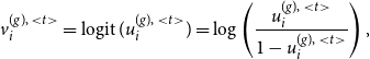 \begin{align*} v_i^{(g), \, \lt t\gt } = \operatorname {logit} (u_i^{(g), \, \lt t\gt }) = \log \left ( \frac {u_i^{(g), \, \lt t\gt }}{1 - u_i^{(g), \, \lt t\gt }} \right ), \end{align*}
then we add a normal term in the form of $v_i^{(g), \, *} = v_i^{(g), \, \lt t\gt } + \operatorname {Normal}(0, \sigma _v^2)$
, and finally we accomplish the retransformation through
$v_i^{(g), \, *} = v_i^{(g), \, \lt t\gt } + \operatorname {Normal}(0, \sigma _v^2)$
, and finally we accomplish the retransformation through
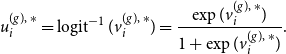 \begin{align*} u_i^{(g), \, *} = \operatorname {logit}^{-1} (v_i^{(g), \, *}) = \frac {\exp (v_i^{(g), \, *})}{1 + \exp (v_i^{(g), \, *})}. \end{align*}
In this setting, the variance $\sigma _v^2$
should be chosen such that a balance between a wide-ranging exploration and a high acceptance rate is achieved, where the relation to the latter also strongly depends on the graphon’s smoothness. Given these formulations, the proposal density can be written as
$\sigma _v^2$
should be chosen such that a balance between a wide-ranging exploration and a high acceptance rate is achieved, where the relation to the latter also strongly depends on the graphon’s smoothness. Given these formulations, the proposal density can be written as
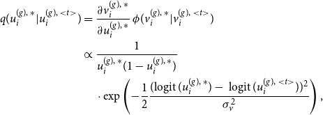 \begin{align*} q(u_i^{(g), \, *} | u^{(g), \, \lt t\gt }_{i}) =& \; \frac {\partial v^{(g), \, *}_i}{\partial u^{(g), \, *}_i} \; \phi (v^{(g), \, *}_i|v^{(g), \, \lt t\gt }_{i}) \\ \propto & \; \frac {1}{u^{(g), \, *}_i (1-u_i^{(g), \, *})} \\ & \;\cdot \exp \left (-\frac {1}{2} \frac {(\text{logit } (u_i^{(g), \, *}) - \text{ logit }(u^{(g), \, \lt t\gt }_{i}))^2}{\sigma _v^2}\right ), \end{align*}
which leads to a proposal ratio of
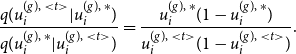 \begin{align*} \frac {q(u^{(g), \, \lt t\gt }_{i} | u^{(g), \, *}_i)}{q(u_i^{(g), \, *}|u^{(g), \, \lt t\gt }_{i})} = \frac {u^{(g), \, *}_i(1-u^{(g), \, *}_i)}{u^{(g), \, \lt t\gt }_{i} (1- u^{(g), \, \lt t\gt }_{i})}. \end{align*}
In combination with the likelihood ratio, the acceptance probability of the proposal, i.e. the probability for setting $u_i^{(g), \, \lt t+1\gt } \,:\!=\, u_i^{(g), \, *}$
, can be calculated through
$u_i^{(g), \, \lt t+1\gt } \,:\!=\, u_i^{(g), \, *}$
, can be calculated through
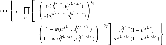 \begin{align*} \min \left \{ 1, \quad \prod _{j \neq i} \left [ \vphantom {\left ( \frac {1-w(u^{(g), \, *}_i, u^{(g), \, \lt t\gt }_{j})}{1-w(u^{(g), \, \lt t\gt }_{i}, u^{(g), \, \lt t\gt }_{j})} \right )^{1-y_{ij}}} \right . \right . & \left . \left . \left ( \frac {w(u_i^{(g), \, *}, u^{(g), \, \lt t\gt }_{j})}{w(u^{(g), \, \lt t\gt }_{i}, u^{(g), \, \lt t\gt }_{j})} \right )^{y_{ij}} \right . \right . \\ \cdot & \left . \left . \left ( \frac {1-w(u^{(g), \, *}_i, u^{(g), \, \lt t\gt }_{j})}{1-w(u^{(g), \, \lt t\gt }_{i}, u^{(g), \, \lt t\gt }_{j})} \right )^{1-y_{ij}} \right ] \frac {u^{(g), \, *}_i(1-u^{(g), \, *}_i)}{u^{(g), \, \lt t\gt }_{i} (1- u^{(g), \, \lt t\gt }_{i})} \right \}. \end{align*}
In case the decision leads to a rejection of the proposal, we set $u_i^{(g), \, \lt t+1\gt } \,:\!=\, u_i^{(g), \, \lt t\gt }$
. To give an intuition about the proposal strategy and how it is affected by
$u_i^{(g), \, \lt t+1\gt } \,:\!=\, u_i^{(g), \, \lt t\gt }$
. To give an intuition about the proposal strategy and how it is affected by $\sigma _v^2$
, Figure 7 shows the proposal density
$\sigma _v^2$
, Figure 7 shows the proposal density $q(\cdot | u^{(g), \, \lt t\gt }_{i})$
and its standard deviation as a function of
$q(\cdot | u^{(g), \, \lt t\gt }_{i})$
and its standard deviation as a function of $u^{(g), \, \lt t\gt }_{i}$
for different values of
$u^{(g), \, \lt t\gt }_{i}$
for different values of $\sigma _v$
. In our studies, we have observed a favorable behavior for the setting
$\sigma _v$
. In our studies, we have observed a favorable behavior for the setting $\sigma _v^2 = 2^2$
.
$\sigma _v^2 = 2^2$
.
Left: proposal density for different current states $u^{(g), \, \lt t\gt }_{i}$
with
$u^{(g), \, \lt t\gt }_{i}$
with $\sigma _v = 1$
. Right: standard deviation of the proposal density against current state
$\sigma _v = 1$
. Right: standard deviation of the proposal density against current state $u^{(g), \, \lt t\gt }_{i}$
; different profiles represent the behavior for different settings of
$u^{(g), \, \lt t\gt }_{i}$
; different profiles represent the behavior for different settings of $\sigma _v$
.
$\sigma _v$
.
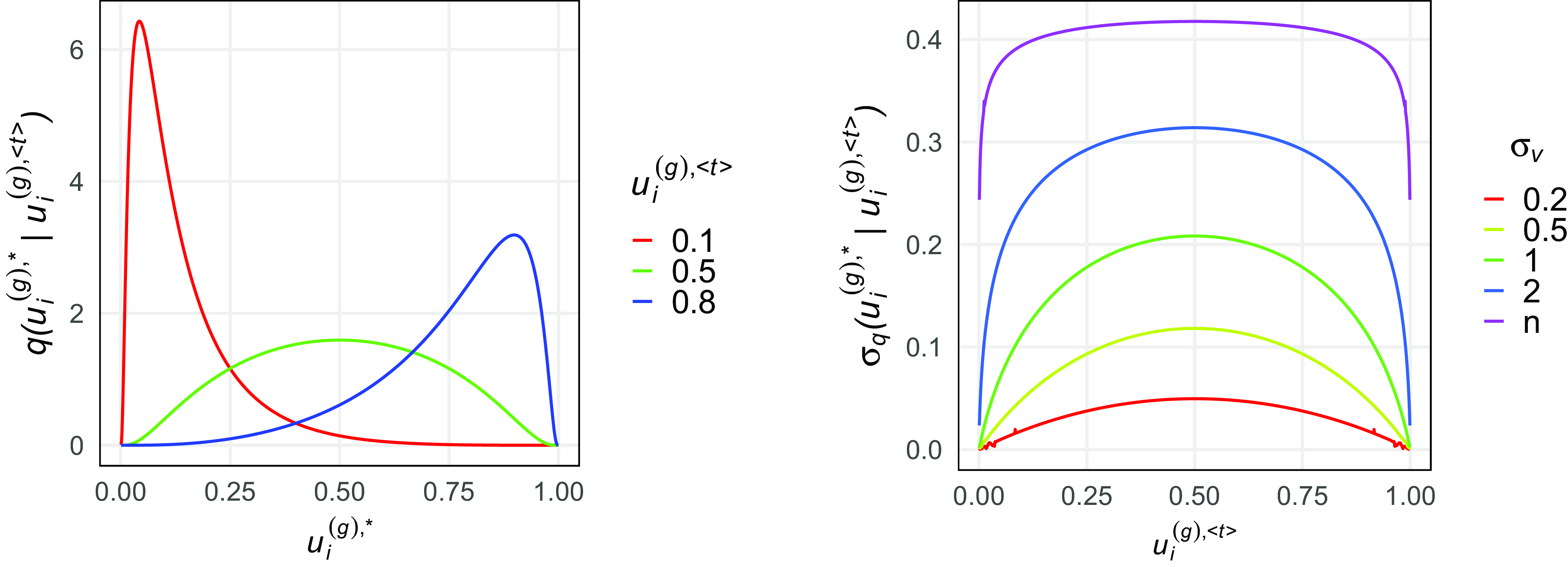
Applying the above updating strategy to all $i = 1,\ldots , N^{(g)}$
completes one overall update. Finally, we achieve a proper Gibbs sampling routine through consecutively repeating this scheme. After cutting the burn-in period and applying an appropriate thinning, this approach yields a sample of the desired joint posterior distribution of the node positions.
$i = 1,\ldots , N^{(g)}$
completes one overall update. Finally, we achieve a proper Gibbs sampling routine through consecutively repeating this scheme. After cutting the burn-in period and applying an appropriate thinning, this approach yields a sample of the desired joint posterior distribution of the node positions.
B. Derivative and penalization of the B-spline function
As has been show in Section 4.2, the log-likelihood of a B-spline function can be straightforwardly extended towards the situation with multiple datasets. Given the formulation from (6), the score function can be calculated as
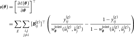 \begin{align*} {\boldsymbol{s}} ( \boldsymbol{\theta }) &= \left [ \frac {\partial \ell (\boldsymbol{\theta })}{\partial \boldsymbol{\theta }} \right ]^\top \\ &= \sum \limits _g \sum \limits _{\substack {i,j \\ j \neq i}} [ {\boldsymbol{B}}_{ij}^{(g)} ]^\top \left ( \frac {y_{ij}^{(g)}}{w_{\boldsymbol{\theta }}^{\text{joint}}(\hat {u}_i^{(g)},\hat {u}_j^{(g)})} - \frac {1-y_{ij}^{(g)}}{1-w_{\boldsymbol{\theta }}^{\text{joint}}(\hat {u}_i^{(g)},\hat {u}_j^{(g)})} \right ) \end{align*}
where the dependence of the graphon on the parameters is expressed as subscript, i.e. $ w_{\boldsymbol{\theta }}(\cdot , \cdot )$
. This, in turn, leads to the Fisher information in the form of
$ w_{\boldsymbol{\theta }}(\cdot , \cdot )$
. This, in turn, leads to the Fisher information in the form of
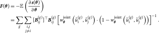 \begin{align*} {\boldsymbol{F}} (\boldsymbol{\theta }) &= - \mathbb{E} \left ( \frac {\partial {\boldsymbol{s}} ( \boldsymbol{\theta })}{\partial \boldsymbol{\theta }} \right ) \\ &= \sum \limits _g \sum \limits _{\substack {i,j \\ j \neq i}} [ {\boldsymbol{B}}_{ij}^{(g)} ]^\top {\boldsymbol{B}}_{ij}^{(g)} \left [ w_{\boldsymbol{\theta }}^{\text{joint}} \left ( \hat {u}_i^{(g)},\hat {u}_j^{(g)} \right ) \cdot \left ( 1 - w_{\boldsymbol{\theta }}^{\text{joint}} \left ( \hat {u}_i^{(g)}, \hat {u}_j^{(g)} \right ) \right ) \right ]^{-1}. \end{align*}
These results can then be used to implement the Fisher scoring procedure, where in (7) we additionally add a penalization term to guarantee a smooth estimation result. For penalizing “neighborhood” elements of the parameter vector $\boldsymbol{\theta } = \left ( \theta _{11},\ldots , \theta _{1L}, \theta _{21}, \ldots , \theta _{LL} \right )^\top$
, the penalization matrix can be formulated through
$\boldsymbol{\theta } = \left ( \theta _{11},\ldots , \theta _{1L}, \theta _{21}, \ldots , \theta _{LL} \right )^\top$
, the penalization matrix can be formulated through
 \begin{equation*} \boldsymbol{P} = \left ( \boldsymbol{J}_L \otimes {\boldsymbol{I}}_L \right )^{\top } \left ( \boldsymbol{J}_L \otimes {\boldsymbol{I}}_L \right ) + \left ( {\boldsymbol{I}}_L \otimes \boldsymbol{J}_L \right )^{\top } \left ( {\boldsymbol{I}}_L \otimes \boldsymbol{J}_L \right ), \end{equation*}
where ${\boldsymbol{I}}_L$
is the identity matrix of size
${\boldsymbol{I}}_L$
is the identity matrix of size $L$
and
$L$
and
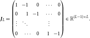 \begin{equation*} \boldsymbol{J}_L = \begin{pmatrix} 1 & -1 & \phantom {-}0 & {\phantom {-}\cdots } & \phantom {-}0 \\ 0 & \phantom {-}1 & -1 & {\phantom {-}\cdots } & \phantom {-}0 \\ \vdots & {\ddots } & & \phantom {-}\vdots \\ 0 & {\phantom {-}\cdots } & \phantom {-}0 & \phantom {-}1 & -1 \\ \end{pmatrix} \in \mathbb{R}^{(L-1) \times L}. \end{equation*}
C. Choosing the number and extent of rectangles
In order to appropriately test null hypothesis (4), in Section 5, we have developed an approach that relies on the partition of the graphon’s domain. According to formulation (8), that involves the number of rectangles, $K$
, as well as their concrete specification in the form of
$K$
, as well as their concrete specification in the form of $[a_{k-1}, a_k) \times [a_{l-1}, a_l)$
. In this regard, we emphasize that two aspects need to be observed. On the one hand, the joint graphon should be approximately constant within rectangles, requiring
$[a_{k-1}, a_k) \times [a_{l-1}, a_l)$
. In this regard, we emphasize that two aspects need to be observed. On the one hand, the joint graphon should be approximately constant within rectangles, requiring $[a_{k-1}, a_k) \times [a_{l-1}, a_l)$
to be not too expansive. On the other hand, the amount of edge variables per network falling into these blocks should be high, which needs rather broad rectangles. Thus, a trade-off between these two opposed requirements should be reached. In general, we choose
$[a_{k-1}, a_k) \times [a_{l-1}, a_l)$
to be not too expansive. On the other hand, the amount of edge variables per network falling into these blocks should be high, which needs rather broad rectangles. Thus, a trade-off between these two opposed requirements should be reached. In general, we choose $K$
to grow more slowly than both network dimensions, e.g. scaling as
$K$
to grow more slowly than both network dimensions, e.g. scaling as $\min _g \sqrt {N^{(g)}}$
. Note that choosing
$\min _g \sqrt {N^{(g)}}$
. Note that choosing $K=1$
would imply to test whether the two networks possess the same global density under the assumption of a joint Erdős–Rényi model. Having determined a suitable value for
$K=1$
would imply to test whether the two networks possess the same global density under the assumption of a joint Erdős–Rényi model. Having determined a suitable value for $K$
, we then simply specify the boundaries of the rectangles through
$K$
, we then simply specify the boundaries of the rectangles through $a_k = k/K$
for
$a_k = k/K$
for $k=0,\ldots ,K$
. In combination with the subsequent adjustment of the latent positions as described in Section 4.1, which leads to equidistance of the estimates
$k=0,\ldots ,K$
. In combination with the subsequent adjustment of the latent positions as described in Section 4.1, which leads to equidistance of the estimates $\hat {u}_i^{(g)}$
, a general lower bound for the amount of contained nodes per interval,
$\hat {u}_i^{(g)}$
, a general lower bound for the amount of contained nodes per interval, $N_k^{(g)}$
, can be derived. To be precise, we can formulate
$N_k^{(g)}$
, can be derived. To be precise, we can formulate
 \begin{multline*} N_k^{(g)} = \left \vert \left \{i \in \{ 1,\ldots , N^{(g)}\}: \frac {i}{N^{(g)} +1} \in [a_{k-1}, a_k) \right \} \right \vert \geq \left \lfloor \frac {1}{K} (N^{(g)} +1) \right \rfloor , \end{multline*}
where $\lfloor x \rfloor$
returns the largest integer smaller than or equal to
$\lfloor x \rfloor$
returns the largest integer smaller than or equal to $x$
. Given that,
$x$
. Given that, $K$
could also be chosen such that, per network, a prescribed minimum amount of edge variables per rectangle (
$K$
could also be chosen such that, per network, a prescribed minimum amount of edge variables per rectangle ( $N_k^{(g)} N_l^{(g)}$
for
$N_k^{(g)} N_l^{(g)}$
for $l \gt k$
and
$l \gt k$
and $N_k^{(g)} (N_k^{(g)}-1)/2$
for
$N_k^{(g)} (N_k^{(g)}-1)/2$
for $l=k$
) is guaranteed.
$l=k$
) is guaranteed.
As a final remark, we emphasize that with regard to the rectangle-based test statistic, it seems natural to alternatively apply a histogram estimator (Chan and Airoldi, Reference Chan and Airoldi2014 or Olhede and Wolfe, Reference Olhede and Wolfe2014). However, the smooth graphon estimation adapted from Sischka and Kauermann (Reference Sischka and Kauermann2024) considers a global node ordering which refers not only to separated intervals but to the entire domain of $[0,1]$
. This consequently facilitates the iterative estimation procedure and thus leads to a more plausible and faster converging node positioning.
$[0,1]$
. This consequently facilitates the iterative estimation procedure and thus leads to a more plausible and faster converging node positioning.
D. Acquiring and processing of brain functional activation data
The data we use for analyzing differences in the functional brain activation are originally provided by the Autism Brain Imaging Data Exchange project (ABIDE I, Reference Abide2013, Di Martino et al., Reference Di Martino, Yan, Li, Denio, Castellanos, Alaerts, Anderson, Assaf, Bookheimer, Dapretto, Deen, Delmonte, Dinstein, Ertl-Wagner, Fair, Gallagher, Kennedy, Keown, Keysers, Lainhart, Lord, Luna, Menon, Minshew, Monk, Mueller, Müller, Nebel, Nigg, O’Hearn, Pelphrey, Peltier, Rudie, Sunaert, Thioux, Tyszka, Uddin, Verhoeven, Wenderoth, Wiggins, Mostofsky and Milham2014). However, we make use of preprocessed data that are directly accessible through the Preprocessed Connectomes Project platform (PCP 2015, Craddock et al., Reference Craddock, Benhajali, Chu, Chouinard, Evans, Jakab, Khundrakpam, Lewis, Li and Milham2013). To be precise, we here apply the Connectome Computation System pipeline (Xu et al., Reference Xu, Yang, Jiang, Xing and Zuo2015) and the reduction to the Automated Anatomical Labeling atlas (Tzourio-Mazoyer et al., Reference Tzourio-Mazoyer, Landeau, Papathanassiou, Crivello, Etard, Delcroix, Mazoyer and Joliot2002). For each participant, this yields a dataset that consists of activity measurements over time for $116$
prespecified brain regions (a.k.a. regions of interest). Based on these temporal activity measurements, we calculate Pearson’s correlation coefficient between all pairs of brain regions which, per participant, leads to the corresponding functional connectivity matrix (Song et al., Reference Song, Epalle and Lu2019, Subbaraju et al., Reference Subbaraju, Suresh, Sundaram and Narasimhan2017). For this analysis, we rely on the data from New York University, comprising
$116$
prespecified brain regions (a.k.a. regions of interest). Based on these temporal activity measurements, we calculate Pearson’s correlation coefficient between all pairs of brain regions which, per participant, leads to the corresponding functional connectivity matrix (Song et al., Reference Song, Epalle and Lu2019, Subbaraju et al., Reference Subbaraju, Suresh, Sundaram and Narasimhan2017). For this analysis, we rely on the data from New York University, comprising $73$
ASD patients and
$73$
ASD patients and $98$
TD subjects. For aggregating these connectivity patterns per clinical group, we apply Fisher’s transformation to the pairwise correlation coefficients, calculate their mean for all pairs of brain regions, and finally retransform these means (Pascual-Belda et al., Reference Pascual-Belda, Díaz-Parra and Moratal2018). This yields for both diagnostic groups a
$98$
TD subjects. For aggregating these connectivity patterns per clinical group, we apply Fisher’s transformation to the pairwise correlation coefficients, calculate their mean for all pairs of brain regions, and finally retransform these means (Pascual-Belda et al., Reference Pascual-Belda, Díaz-Parra and Moratal2018). This yields for both diagnostic groups a $116 \times 116$
weighted connectivity matrix which we binarize by employing a threshold of
$116 \times 116$
weighted connectivity matrix which we binarize by employing a threshold of $0.4$
. Based on that, the two final networks we obtain both possess a global density of about
$0.4$
. Based on that, the two final networks we obtain both possess a global density of about $30\%$
. With regard to the choice of the threshold, Song et al. (Reference Song, Epalle and Lu2019) have found that this has only minor effects when comparing the networks.
$30\%$
. With regard to the choice of the threshold, Song et al. (Reference Song, Epalle and Lu2019) have found that this has only minor effects when comparing the networks.


 Open access