


1. Introduction
In its simplest form, a network is a static collection of nodes joined together by edges. Ties between nodes can be directed or undirected and can be dichotomous or valued, and different kinds of ties may function differently. Networks can be interpersonal, micro-level networks where nodes represent individual actors, or inter-organizational, macro-level networks where nodes represent organizations (Chen et al., Reference Chen, Mehra, Tasselli and Borgatti2022). Broadly speaking, networks capture the pattern of interactions between elements of a system, reducing the system to a basic topological structure that facilitates analysis. Network variables can serve as both dependent (outcome) and independent (explanatory) variables (Borgatti and Foster, Reference Borgatti and Foster2003). Furthermore, research can focus on the impact of individual dyads, or take a whole-of-network approach (Provan et al., Reference Provan, Fish and Sydow2007).
Networks that change over time, or temporal networks, can model both changes in relational states (i.e., the formation, transformation, or dissolution of a tie) and the occurrence of relational events (i.e., transactional events occurring between two actors) (Chen et al., Reference Chen, Mehra, Tasselli and Borgatti2022). In this paper, we present the temporal configuration model (TCM), a simple yet flexible way to model temporal networks. This approach can be used to model networks where edges represent relational states or where ties denote relational events. Furthermore, it can be applied to a diverse set of open research questions, including studying the mechanisms of network dynamics, the outcomes of network dynamics, and the interplay of relational states and relational events (Chen et al., Reference Chen, Mehra, Tasselli and Borgatti2022).
Over the last decade, temporal networks have emerged as a fascinating topic that has received substantial research interest from a variety of disciplines. The majority of research focuses on developing various temporal models that describe real-world data. Popular approaches include dynamic link modeling, activity-driven modeling, link-node memory modeling, and community dynamics modeling (Holme, Reference Holme2013; Perra et al., Reference Perra, Gonçalves, Pastor-Satorras and Vespignani2012; Vestergaard et al., Reference Vestergaard, Génois and Barrat2014; Peixoto and Rosvall, Reference Peixoto and Rosvall2017). These models provide key insights into the mechanisms of network dynamics, that is, how network ties form, dissolve, and evolve. A related line of research, relational event models (REMs), focuses on the intensity and sequencing of relational events (Butts, Reference Butts2008; Butts et al., Reference Butts, Lomi, Snijders and Stadtfeld2023). While REMs are useful for studying specific event-based processes and the timing of interactions, they do not directly capture tie persistence or larger-scale structural change. Stochastic actor-oriented models (SAOMs) provide another influential framework, modeling micro-mechanisms of tie formation and dissolution, but their estimation relies on extensive simulations and repeated full-network observations (Snijders, Reference Snijders2001; Snijders et al., Reference Snijders, Van de Bunt and Steglich2010). Dynamic random graph approaches, such as Zhang et al., propose generative rules where edges form and dissolve at constant rates and provide estimators for those rates (Zhang et al., Reference Zhang, Moore and Newman2017). Together, these approaches illustrate the progress of temporal network modeling, but a common limitation is that their theoretical guarantees may fail when complete sequences of network snapshots are unavailable, a situation often encountered in empirical applications where networks are only partially observed or aggregated over time.
Our proposed TCM addresses this limitation by allowing more freedom in how edges are formed and dissolved through the flexibility of CM degree distributions with an explicit mechanism for tie persistence. At the same time, it provides explicit, consistent estimators that clarify how much temporal network information is required to reliably estimate model parameters from data. Beyond its theoretical contribution, the TCM is also relevant to applications where tie persistence is essential, such as biological networks, human mobility and communication networks, and financial systems (Barabasi and Oltvai, Reference Barabasi and Oltvai2004; Barbosa et al., Reference Barbosa, Barthelemy, Ghoshal, James, Lenormand, Louail and Tomasini2018; Karsai et al., Reference Karsai, Jo and Kimmo2018; Barucca and Lillo, Reference Barucca and Lillo2016).
We also present an application of our model to infectious disease modeling on interpersonal networks. When a network evolves slowly relative to a spreading process, the dynamics can be approximated using a static network. When a network evolves very rapidly relative to the spreading process, the dynamics can be approximated well by a time-averaged version of the network. However, when the network and spreading process evolve at comparable time scales, the interplay between the two becomes important (Holme and Saramäki, Reference Holme and Saramäki2012; Holme, Reference Holme2015; Holme and Saramäki, Reference Holme and Saramäki2019; Jordan et al., Reference Jordan, Winer and Salem2020; Hosseinzadeh et al., Reference Hosseinzadeh, Cannataro, Guzzi and Dondi2022). Thus, regardless of whether one studies the spread of infectious disease, health behaviors, or information, it is essential that the model capture important temporal changes in the underlying network topology.
Recent technological advances have made high-fidelity individual-level proximity data easier to capture, thereby allowing us to study empirical time-varying networks more precisely. Wearable sensors, like RFID tags and Bluetooth-enabled devices, such as smartphones, allow researchers to collect accurate, granular data in a passive manner (Vanhems et al., Reference Vanhems, Barrat, Cattuto, Pinton, Khanafer, Régis, Kim, Comte and Voirin2013; Sapiezynski et al., Reference Sapiezynski, Stopczynski, Lassen and Lehmann2019; Neto et al., Reference Neto, Haenni, Phuka, Ozella, Paolotti, Cattuto, Robles and Lichand2021). These technologies also allow investigators to capture proximity information with high precision, measuring the exact time and duration that two individuals are in close contact, along with their approximate distance from one another. This high-fidelity data allows us to quantify exposure, making it ideal for studying the spread of contagion. However, this begs the question: how much temporal granularity is needed to accurately capture spreading processes over networks? Very granular temporal resolution poses its own challenges, as it may capture unimportant interactions and erode privacy-protecting measures. Coarser collection can help preserve privacy and be less burdensome to store and analyze. However, if the network information is too coarse, we may miss key temporal dynamics, thereby inhibiting our ability to accurately model spreading processes over the network.
The remainder of the paper is organized as follows. In Section 2, we present a generative model for temporal networks which employs an edge persistence rate, which can be a simple constant, generated from a distribution, or some function of the empirical data. We then establish consistent estimators for the model parameters. Under the proposed modeling framework, the temporal granularity required for a consistent estimator depends on the number of edges that persist up to
 $ k$
time steps from the original network, where
$ k$
time steps from the original network, where
 $ k$
corresponds to the highest moment of the generating distribution we seek to estimate. For instance, if the generating distribution is Normal or Beta, then only
$ k$
corresponds to the highest moment of the generating distribution we seek to estimate. For instance, if the generating distribution is Normal or Beta, then only
 $k=2$
is required, since the first and second moments alone suffice to characterize the distribution. We find that constructing an estimator using as much temporal network information as possible does not necessarily result in a superior estimator. Section 3 presents a simulation that illustrates some of the key statistical properties of our proposed estimators. In Section 4, we derive some theoretical results for a spreading process on temporal configuration networks, with a specific focus on the reproduction number, a fundamental concept in infectious disease epidemiology. In Section 5, we demonstrate how to fit the proposed model to an empirical dataset in the context of an infectious disease spreading through student contact on a college campus. Finally, Section 6 summarizes the main contributions of the study and suggests avenues for future research.
$k=2$
is required, since the first and second moments alone suffice to characterize the distribution. We find that constructing an estimator using as much temporal network information as possible does not necessarily result in a superior estimator. Section 3 presents a simulation that illustrates some of the key statistical properties of our proposed estimators. In Section 4, we derive some theoretical results for a spreading process on temporal configuration networks, with a specific focus on the reproduction number, a fundamental concept in infectious disease epidemiology. In Section 5, we demonstrate how to fit the proposed model to an empirical dataset in the context of an infectious disease spreading through student contact on a college campus. Finally, Section 6 summarizes the main contributions of the study and suggests avenues for future research.
2. Temporal network model
2.1 Model specification
The configuration model (CM) is a widely used network model as it balances both realism and simplicity (Newman, Reference Newman2018; Holme and Saramäki, Reference Holme and Saramäki2012; Fosdick et al., Reference Fosdick, Larremore, Nishimura and Ugander2018). Unlike many other network models, the CM incorporates arbitrary degree distributions. The exact degree of each individual node is fixed, which in turn fixes the total number of edges. To construct a network realization from a CM, one first specifies the total number of nodes in the network, denoted
 $N$
. Then, for a given node
$N$
. Then, for a given node
 $i$
, one specifies the degree of that node,
$i$
, one specifies the degree of that node,
 $k_{i}$
, repeating this process for all nodes in the network. Each node is then given “stubs” equal to its degree, where a stub is simply an edge that is only connected to the node in question with its remaining end free. Pairs of stubs are then selected uniformly at random and connected to form edges until no stubs remain. The CM has several attractive properties. First, each possible matching of stubs is generated with equal probability. Specifically, the probability of nodes
$k_{i}$
, repeating this process for all nodes in the network. Each node is then given “stubs” equal to its degree, where a stub is simply an edge that is only connected to the node in question with its remaining end free. Pairs of stubs are then selected uniformly at random and connected to form edges until no stubs remain. The CM has several attractive properties. First, each possible matching of stubs is generated with equal probability. Specifically, the probability of nodes
 $i$
and
$i$
and
 $j$
being connected is given by
$j$
being connected is given by
 $\frac {k_{i}k_{j}}{2m-1}$
, where
$\frac {k_{i}k_{j}}{2m-1}$
, where
 $m$
is the total number of edges. Because any stub is equally likely to be connected to any other, many of the properties of the CM can be solved exactly. While the CM does allow for multi-edges and self-edges, their probability tends to zero as
$m$
is the total number of edges. Because any stub is equally likely to be connected to any other, many of the properties of the CM can be solved exactly. While the CM does allow for multi-edges and self-edges, their probability tends to zero as
 $N$
approaches infinity. The CM is recognized as “one of the most important theoretical models in the study of networks” and many consider it one of the canonical network models (Newman, Reference Newman2018). When studying a new question or process, the CM is often the first model network scientists employ, making it an ideal foundation for our temporal network model (Newman, Reference Newman2018; Fosdick et al., Reference Fosdick, Larremore, Nishimura and Ugander2018).
$N$
approaches infinity. The CM is recognized as “one of the most important theoretical models in the study of networks” and many consider it one of the canonical network models (Newman, Reference Newman2018). When studying a new question or process, the CM is often the first model network scientists employ, making it an ideal foundation for our temporal network model (Newman, Reference Newman2018; Fosdick et al., Reference Fosdick, Larremore, Nishimura and Ugander2018).
We present a time-varying version of the CM that we call the TCM. Like the CM, the TCM allows for an arbitrary degree distribution. Additionally, it encodes persistent ties, a key motivation for using and studying network models, by assigning each dyad a latent persistence probability.
To construct a TCM, one creates an initial network,
 $G_{0}$
, via the standard CM algorithm. At each subsequent discrete time point
$G_{0}$
, via the standard CM algorithm. At each subsequent discrete time point
 $t$
, a new network,
$t$
, a new network,
 $G_{t}$
, is generated as follows. For each edge in
$G_{t}$
, is generated as follows. For each edge in
 $G_{t-1}$
, a Bernoulli trial is conducted with success probability equal to that edge’s latent persistence probability. That is, for an edge between nodes
$G_{t-1}$
, a Bernoulli trial is conducted with success probability equal to that edge’s latent persistence probability. That is, for an edge between nodes
 $i$
and
$i$
and
 $j$
, we perform a Bernoulli trial with success probability
$j$
, we perform a Bernoulli trial with success probability
 $p_{ij}$
. If the trial results in a success, the edge remains. If the trial is unsuccessful, the edge is broken, creating two stubs. After Bernoulli trials have been completed for all edges in
$p_{ij}$
. If the trial results in a success, the edge remains. If the trial is unsuccessful, the edge is broken, creating two stubs. After Bernoulli trials have been completed for all edges in
 $G_{t-1}$
, stubs are matched uniformly at random with one another, forming edges in the new network,
$G_{t-1}$
, stubs are matched uniformly at random with one another, forming edges in the new network,
 $G_{t}$
. This process is repeated for each time step until one obtains the desired sequence of graphs,
$G_{t}$
. This process is repeated for each time step until one obtains the desired sequence of graphs,
 $G_{0}, G_{1}, \ldots , G_{T}$
.
$G_{0}, G_{1}, \ldots , G_{T}$
.
The TCM can take on several intuitive forms by adjusting the latent edge-wise persistence probability. We begin by considering the two extremes. First, we can recover the standard CM simply by setting
 $p_{ij}=1$
for all
$p_{ij}=1$
for all
 $i$
,
$i$
,
 $j$
. This creates a static network such that
$j$
. This creates a static network such that
 $G_{t}=G_{0}$
for all times
$G_{t}=G_{0}$
for all times
 $t$
. Second, if we set
$t$
. Second, if we set
 $p_{ij}=0$
for all
$p_{ij}=0$
for all
 $i$
,
$i$
,
 $j$
, we simply generate independent and identically distributed random draws of graphs from a CM ensemble. At each
$j$
, we simply generate independent and identically distributed random draws of graphs from a CM ensemble. At each
 $t$
, a CM with the specified number of nodes and degree sequence will be generated, but this instance will be independent of the previous network realizations.
$t$
, a CM with the specified number of nodes and degree sequence will be generated, but this instance will be independent of the previous network realizations.
A more interesting scenario is obtained by setting
 $p_{ij}$
equal to some fixed
$p_{ij}$
equal to some fixed
 $p \in (0,1)$
for all pairs
$p \in (0,1)$
for all pairs
 $i$
,
$i$
,
 $j$
. That is, we specify a single or homogeneous persistence probability for all edges in the network. This parameter dictates how quickly the network changes over time. If
$j$
. That is, we specify a single or homogeneous persistence probability for all edges in the network. This parameter dictates how quickly the network changes over time. If
 $p$
is large, the network will change slowly as edges are highly likely to persist forward in time. If
$p$
is large, the network will change slowly as edges are highly likely to persist forward in time. If
 $p$
is small, the network will change rapidly.
$p$
is small, the network will change rapidly.
If we wanted the persistence probability to vary across the network, creating a more heterogeneous population, we can draw edge-level probabilities from some distribution for all node pairs. We could also imagine circumstances where it may make sense to encode some functional form for
 $p_{ij}$
. For instance, edge-level persistence probabilities could be a function of node-level attributes if such information is available. We could envision a scenario where some individuals are more likely to stay within a particular social group while others may frequently move between groups, be it due to age, location, or some other factor or combination of factors. In this setting, we might construct
$p_{ij}$
. For instance, edge-level persistence probabilities could be a function of node-level attributes if such information is available. We could envision a scenario where some individuals are more likely to stay within a particular social group while others may frequently move between groups, be it due to age, location, or some other factor or combination of factors. In this setting, we might construct
 $p_{ij}$
to be some function of node
$p_{ij}$
to be some function of node
 $i$
’s attributes,
$i$
’s attributes,
 $a_{i}$
, and node
$a_{i}$
, and node
 $j$
’s attributes,
$j$
’s attributes,
 $a_{j}$
. As such, every edge would have a distinct probability that would relate back to the two individuals in question. We could take this one step further and have edge-level persistence probabilities be a function of the relationship between the two nodes. For example, edges between close friends may have a higher persistence probability than those between acquaintances.
$a_{j}$
. As such, every edge would have a distinct probability that would relate back to the two individuals in question. We could take this one step further and have edge-level persistence probabilities be a function of the relationship between the two nodes. For example, edges between close friends may have a higher persistence probability than those between acquaintances.
2.2 Inference
We focus on three of the intuitive forms outlined above, namely a single persistence probability for the entire network, edge-level persistence parameters drawn from a probability distribution, and edge-level persistence parameters that are product of node-level persistence parameters drawn from a probability distribution. In the first model, the entire network has a single persistence probability,
 $p$
. We then consider the case where the persistence rate
$p$
. We then consider the case where the persistence rate
 $p_{ij}$
of edge
$p_{ij}$
of edge
 $(i,j)$
is generated from a given distribution
$(i,j)$
is generated from a given distribution
 $W$
, that is,
$W$
, that is,
 $p_{ij}\sim W$
, for all
$p_{ij}\sim W$
, for all
 $i$
,
$i$
,
 $j$
. Finally, we consider the case where
$j$
. Finally, we consider the case where
 $p_{ij} = p_{i}p_{j}$
, where
$p_{ij} = p_{i}p_{j}$
, where
 $p_i \sim W$
, for
$p_i \sim W$
, for
 $i = 1,\cdots , N$
are independently drawn from a given distribution
$i = 1,\cdots , N$
are independently drawn from a given distribution
 $W$
. Notice that the first model is a special case of the second model as the distribution
$W$
. Notice that the first model is a special case of the second model as the distribution
 $W$
shrinks to a constant
$W$
shrinks to a constant
 $p$
.
$p$
.
We observe that the future status of each edge after one step follows a Bernoulli distribution with mean equal to the persistence rate of that edge, and the status of each edge after two time steps follows a Bernoulli distribution with mean equal to the square of the persistence rate. The number of edges remaining after one or two time steps in the network is the sum of independent Bernoulli distributions. Thus, to estimate the first moment of the distribution, we can simply use the proportion of edges persisted one time step. To estimate the second moment of the distribution, we can use the proportion of edges that persisted two time steps. Next, we show that these estimators are consistent for each scenario.
Remark: As long as
 $W$
is uniquely determined from its first
$W$
is uniquely determined from its first
 $k$
moments, the proposed approach can specify the distribution of
$k$
moments, the proposed approach can specify the distribution of
 $W$
.
$W$
.
Model 1: All edges of the network have a single persistence probability
 $p$
for some
$p$
for some
 $0 \leq p \leq 1$
.
$0 \leq p \leq 1$
.
Let
 $X_{0} = x_0$
denote the number of edges in the initial graph,
$X_{0} = x_0$
denote the number of edges in the initial graph,
 $G_{0}$
. Notice that
$G_{0}$
. Notice that
 $x_0$
is a fixed constant for a given initial graph
$x_0$
is a fixed constant for a given initial graph
 $G_0$
. Let
$G_0$
. Let
 $X_{1}$
denote the number of edges that persist to time
$X_{1}$
denote the number of edges that persist to time
 $t = 1$
. That is,
$t = 1$
. That is,
 $X_{1} = \sum _{(i,j) \in G_0} \text{Bernoulli}(p)$
. We can then use the ratio
$X_{1} = \sum _{(i,j) \in G_0} \text{Bernoulli}(p)$
. We can then use the ratio
 $Z_{1}=\frac {X_{1}}{X_{0}}$
to estimate the persistence probability
$Z_{1}=\frac {X_{1}}{X_{0}}$
to estimate the persistence probability
 $p$
. Lemma 2.1 gives the properties of estimator
$p$
. Lemma 2.1 gives the properties of estimator
 $Z_1$
; the proof can be found in Appendix A.
$Z_1$
; the proof can be found in Appendix A.
Lemma 2.1.
 $\ \frac {Z_1 -p}{\sqrt {\big ( p(1-p)\big )/X_0}}$
converges to a standard normal distribution, as
$\ \frac {Z_1 -p}{\sqrt {\big ( p(1-p)\big )/X_0}}$
converges to a standard normal distribution, as
 $X_0 \rightarrow \infty$
.
$X_0 \rightarrow \infty$
.
Since the network continues to evolve over time, we can incorporate this information to refine our estimate of
 $p$
. Following the same logic as in Lemma 2.1, we can show that the ratio of edges remaining after each time step is also an unbiased and consistent estimator of
$p$
. Following the same logic as in Lemma 2.1, we can show that the ratio of edges remaining after each time step is also an unbiased and consistent estimator of
 $p$
. To obtain a more precise estimator for the persistence probability
$p$
. To obtain a more precise estimator for the persistence probability
 $p$
, we can use the average of ratios over all time steps, denoted
$p$
, we can use the average of ratios over all time steps, denoted
 $\bar {Z}$
.
$\bar {Z}$
.
Before discussing the proposed estimator
 $\bar {Z}$
, we first walk through the evolution of the temporal network and set up the necessary notation. During the first time step, the broken edges of the original network
$\bar {Z}$
, we first walk through the evolution of the temporal network and set up the necessary notation. During the first time step, the broken edges of the original network
 $G_0$
form stubs and are rematched to create new edges. Let
$G_0$
form stubs and are rematched to create new edges. Let
 $Y_{1}$
denote the number of newly formed edges (excluding self-loops and multi-edges) at
$Y_{1}$
denote the number of newly formed edges (excluding self-loops and multi-edges) at
 $t=1$
. For large networks, the number of self-loops and multi-edges is negligible relative to the total number of edges; thus,
$t=1$
. For large networks, the number of self-loops and multi-edges is negligible relative to the total number of edges; thus,
 $Y_{1}=X_{0}-X_{1}+o(1)$
, where
$Y_{1}=X_{0}-X_{1}+o(1)$
, where
 $o(1)$
captures the number of self-loops and multi-edges. Let
$o(1)$
captures the number of self-loops and multi-edges. Let
 $X_{1}^{+}$
denote the total number of edges at
$X_{1}^{+}$
denote the total number of edges at
 $t = 1$
after adding the new edges to the remaining edges. That is,
$t = 1$
after adding the new edges to the remaining edges. That is,
 $X_{1}^{+}=X_{1}+Y_{1} = X_{0} + o(1)$
. Then, at
$X_{1}^{+}=X_{1}+Y_{1} = X_{0} + o(1)$
. Then, at
 $t = 2$
, the number of edges that persist is
$t = 2$
, the number of edges that persist is
 $X_{2}\sim$
Binomial
$X_{2}\sim$
Binomial
 $(X_{1}^{+},p)$
and the total number of edges after the rematching is
$(X_{1}^{+},p)$
and the total number of edges after the rematching is
 $X_{2}^{+}=X_{1}^{+}+o(1)$
. Similarly, for time
$X_{2}^{+}=X_{1}^{+}+o(1)$
. Similarly, for time
 $t = T$
,
$t = T$
,
 $X_{T}$
is the total number of edges persisting from
$X_{T}$
is the total number of edges persisting from
 $X_{T-1}^{+}$
and
$X_{T-1}^{+}$
and
 $X_{T}^{+}$
is the number of edges after the rematching.
$X_{T}^{+}$
is the number of edges after the rematching.
Let
 $Z_{t}$
denote the fraction of edges that persist to time
$Z_{t}$
denote the fraction of edges that persist to time
 $t$
, that is,
$t$
, that is,
 $Z_{t}=\frac {X_{t}}{X_{t-1}^{+}}$
, for
$Z_{t}=\frac {X_{t}}{X_{t-1}^{+}}$
, for
 $t = 1,\cdots ,T$
. Then the proposed estimator
$t = 1,\cdots ,T$
. Then the proposed estimator
 $\bar {Z}$
is defined as
$\bar {Z}$
is defined as
 $\bar {Z}=\frac {1}{T}\left (Z_{1}+Z_{2}+\cdots +Z_{T}\right ).$
Next, we present some important properties of the proposed estimator
$\bar {Z}=\frac {1}{T}\left (Z_{1}+Z_{2}+\cdots +Z_{T}\right ).$
Next, we present some important properties of the proposed estimator
 $\bar {Z}$
, with a proof provided in Appendix B.
$\bar {Z}$
, with a proof provided in Appendix B.
Theorem 2.2.
The estimator
 $\bar {Z}$
is an unbiased and consistent estimator of the persistence probability
$\bar {Z}$
is an unbiased and consistent estimator of the persistence probability
 $p$
. In addition, when
$p$
. In addition, when
 $T = o(X_0)$
and
$T = o(X_0)$
and
 $T\rightarrow \infty$
,
$T\rightarrow \infty$
,
 $\bar {Z}$
converges to
$\bar {Z}$
converges to
 $p$
at the rate of
$p$
at the rate of
 $O_p\left (\sqrt {\frac {1}{X_0}} (\frac {1}{T})^{1/2-\delta }\right )$
, for some small
$O_p\left (\sqrt {\frac {1}{X_0}} (\frac {1}{T})^{1/2-\delta }\right )$
, for some small
 $\delta \gt 0$
.
$\delta \gt 0$
.
Remark: From Theorem 2.1 and Lemma 2.1, we see that by incorporating information about network evolution over time, the estimator
 $\bar {Z}$
converges to the persistence probability
$\bar {Z}$
converges to the persistence probability
 $p$
faster than
$p$
faster than
 $Z_1$
by a factor of
$Z_1$
by a factor of
 $(\frac {1}{T})^{1/2-\delta }$
for some small positive
$(\frac {1}{T})^{1/2-\delta }$
for some small positive
 $\delta$
.
$\delta$
.
Model 2: Now, consider drawing
 $p_{ij}$
from a given distribution
$p_{ij}$
from a given distribution
 $W$
, that is,
$W$
, that is,
 $p_{ij}\sim W$
for all
$p_{ij}\sim W$
for all
 $i$
,
$i$
,
 $j$
. The simplest way to structure this model is to set the persistence probability for edge
$j$
. The simplest way to structure this model is to set the persistence probability for edge
 $(i,j)$
as
$(i,j)$
as
 $p_{ij}$
, fixing it over time. Alternatively, one could fix the persistence probability of an edge over a time window of
$p_{ij}$
, fixing it over time. Alternatively, one could fix the persistence probability of an edge over a time window of
 $T_{0}$
time steps for some
$T_{0}$
time steps for some
 $T_{0}\gt 1$
. Under this model, edge persistence probabilities are regenerated from
$T_{0}\gt 1$
. Under this model, edge persistence probabilities are regenerated from
 $W$
anew for each time window. This latter approach may be more realistic in some settings.
$W$
anew for each time window. This latter approach may be more realistic in some settings.
We will show that in either case the ratio of edges remaining after the first time step from the original network
 $G_0$
and the ratio of edges remaining after the first two steps from the original network
$G_0$
and the ratio of edges remaining after the first two steps from the original network
 $G_0$
can serve as good estimators for the first and second moment of the distribution
$G_0$
can serve as good estimators for the first and second moment of the distribution
 $W$
, respectively. For simplicity, we only provide the proofs for the estimator of the first moment; the proof for the estimator of the second moment is similar. Recycling the notation from Model 1, we will use
$W$
, respectively. For simplicity, we only provide the proofs for the estimator of the first moment; the proof for the estimator of the second moment is similar. Recycling the notation from Model 1, we will use
 $Z_1 = \frac {X_1}{X_0}$
to estimate the first moment
$Z_1 = \frac {X_1}{X_0}$
to estimate the first moment
 $E(W)$
. Lemma 2.3 gives us the convergence property of the estimator
$E(W)$
. Lemma 2.3 gives us the convergence property of the estimator
 $Z_1$
; the proof is provided in Appendix C.
$Z_1$
; the proof is provided in Appendix C.
Lemma 2.3.
 $Z_1$
is an unbiased and consistent estimator of the first moment
$Z_1$
is an unbiased and consistent estimator of the first moment
 $E(W)$
of distribution
$E(W)$
of distribution
 $W$
, as
$W$
, as
 $X_0 \rightarrow \infty$
.
$X_0 \rightarrow \infty$
.
Next, we consider how to utilize temporal network information to refine the estimator
 $Z_1$
. Consider the case where we generate
$Z_1$
. Consider the case where we generate
 $p_{ij}$
from distribution
$p_{ij}$
from distribution
 $W$
and assign fixed persistence probabilities
$W$
and assign fixed persistence probabilities
 $p_{ij}$
for the
$p_{ij}$
for the
 $(i,j)$
dyad. In this case,
$(i,j)$
dyad. In this case,
 $\bar {Z}$
, constructed under Model 1, will not be a good estimator for the first moment
$\bar {Z}$
, constructed under Model 1, will not be a good estimator for the first moment
 $E(W)$
of
$E(W)$
of
 $W$
. As the network evolves, edges with higher persistence probabilities are more likely to be retained in the network. Therefore, over time, the persistence probabilities of edges remaining in the network will represent a shifted version of the original distribution
$W$
. As the network evolves, edges with higher persistence probabilities are more likely to be retained in the network. Therefore, over time, the persistence probabilities of edges remaining in the network will represent a shifted version of the original distribution
 $W$
. As a result, using the estimator
$W$
. As a result, using the estimator
 $\bar {Z}$
will result in a biased estimate of
$\bar {Z}$
will result in a biased estimate of
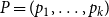
 $E(W)$
. Figure 1 shows this phenomenon, where the initial network has
$E(W)$
. Figure 1 shows this phenomenon, where the initial network has
 $1000$
nodes and the edge persistence probabilities are generated from
$1000$
nodes and the edge persistence probabilities are generated from
 $W = \text{Beta}(4,1)$
for the first time steps. After
$W = \text{Beta}(4,1)$
for the first time steps. After
 $100$
time steps, edge persistence probabilities of edges retained in the network are shifted compared with the original distribution significantly.
$100$
time steps, edge persistence probabilities of edges retained in the network are shifted compared with the original distribution significantly.
Box plots of edge persistence probabilities at the first step and the last step (step 100) for persistence edges of a network of size
 $1000$
over
$1000$
over
 $100$
time steps. Edge persistent probabilities are generated from a
$100$
time steps. Edge persistent probabilities are generated from a
 $\text{Beta}(4,1)$
distribution.
$\text{Beta}(4,1)$
distribution.

Next, consider the variant of Model 2 where the edge persistence probabilities are generated anew from
 $W$
for each time window
$W$
for each time window
 $T_0$
and kept fixed for each edge throughout each time window. More specifically, starting with
$T_0$
and kept fixed for each edge throughout each time window. More specifically, starting with
 $X_0$
edges from the set of edges
$X_0$
edges from the set of edges
 $\boldsymbol{A}_0$
in the initial graph
$\boldsymbol{A}_0$
in the initial graph
 $G_0$
at time
$G_0$
at time
 $t=0$
, we generate persistence probabilities
$t=0$
, we generate persistence probabilities
 $p_{ij}^{(0)}, i,j = 1,\cdots , N$
from a distribution
$p_{ij}^{(0)}, i,j = 1,\cdots , N$
from a distribution
 $W$
and assign the probability
$W$
and assign the probability
 $p_{ij}^{(0)}$
to the edge
$p_{ij}^{(0)}$
to the edge
 $(i,j)$
if the edge appears at time
$(i,j)$
if the edge appears at time
 $t = 0$
and persists to time
$t = 0$
and persists to time
 $T_0-1$
. At time step
$T_0-1$
. At time step
 $T_0$
, persistence probabilities
$T_0$
, persistence probabilities
 $p_{ij}^{(1)}, i,j = 1,\cdots , N$
are generated anew from
$p_{ij}^{(1)}, i,j = 1,\cdots , N$
are generated anew from
 $W$
and assigned to the edge
$W$
and assigned to the edge
 $(i,j)$
if the edge appears at time
$(i,j)$
if the edge appears at time
 $t = T_0$
and persists to time
$t = T_0$
and persists to time
 $2T_0 - 1$
. This process continues until we reach the desired number of time steps
$2T_0 - 1$
. This process continues until we reach the desired number of time steps
 $T$
. If additional information is available regarding the time window
$T$
. If additional information is available regarding the time window
 $T_0$
, we can use information from the first
$T_0$
, we can use information from the first
 $k$
time steps (
$k$
time steps (
 $k \lt T_0$
) from each window to obtain a better estimator for the first
$k \lt T_0$
) from each window to obtain a better estimator for the first
 $k$
moments of distribution
$k$
moments of distribution
 $W$
.
$W$
.
Denote the set of edges of
 $\boldsymbol{A}_0$
that persist to
$\boldsymbol{A}_0$
that persist to
 $t=1$
as
$t=1$
as
 $\boldsymbol{A}_1$
. After the rematching process at
$\boldsymbol{A}_1$
. After the rematching process at
 $t=1$
, the set of edges now becomes
$t=1$
, the set of edges now becomes
 $\boldsymbol{A}_1^+$
. Let
$\boldsymbol{A}_1^+$
. Let
 $X_1$
denote the number of edges in
$X_1$
denote the number of edges in
 $\boldsymbol{A}_1$
and
$\boldsymbol{A}_1$
and
 $X_1^+$
the number of edges in
$X_1^+$
the number of edges in
 $\boldsymbol{A}_1^+$
and so on for
$\boldsymbol{A}_1^+$
and so on for
 $t = 2,\cdots , T$
. Let
$t = 2,\cdots , T$
. Let
 $\mathcal{F}_{k}^+$
denote the
$\mathcal{F}_{k}^+$
denote the
 $\sigma -$
algebra generated by all sets of edges up to time
$\sigma -$
algebra generated by all sets of edges up to time
 $k$
, that is,
$k$
, that is,
 $\mathcal{F}_{k}^+ = \sigma \{\boldsymbol{A}_{1}^+, \ldots , \boldsymbol{A}_{k}^+\}$
. Finally, let
$\mathcal{F}_{k}^+ = \sigma \{\boldsymbol{A}_{1}^+, \ldots , \boldsymbol{A}_{k}^+\}$
. Finally, let
 $Z_k$
represent the fraction of edges remaining after one time step starting from each time window, that is,
$Z_k$
represent the fraction of edges remaining after one time step starting from each time window, that is,
 $Z_1 = \frac {X_1}{X_0}, Z_2 = \frac {X_{T_0+1}}{X_{T_0}^+}, Z_3 = \frac {X_{2T_0+1}}{X_{2T_0}^+}, \cdots$
. Then we can use
$Z_1 = \frac {X_1}{X_0}, Z_2 = \frac {X_{T_0+1}}{X_{T_0}^+}, Z_3 = \frac {X_{2T_0+1}}{X_{2T_0}^+}, \cdots$
. Then we can use
 $\bar {Z} = \sum _{k=1}^{m} Z_k/T$
to estimate the first moment
$\bar {Z} = \sum _{k=1}^{m} Z_k/T$
to estimate the first moment
 $E(W)$
, where
$E(W)$
, where
 $m = [T/T_0]$
.
$m = [T/T_0]$
.
Theorem 2.4.
If the periodic time interval
 $T_0$
is correctly specified, the proposed estimator
$T_0$
is correctly specified, the proposed estimator
 $\bar {Z}$
is an unbiased and consistent estimator for
$\bar {Z}$
is an unbiased and consistent estimator for
 $E(W)$
. In addition, when
$E(W)$
. In addition, when
 $T = o(X_0)$
and
$T = o(X_0)$
and
 $T\rightarrow \infty$
,
$T\rightarrow \infty$
,
 $\bar {Z}$
converges to
$\bar {Z}$
converges to
 $E(W)$
at the rate of
$E(W)$
at the rate of
 $O_p\left (\sqrt {\frac {1}{X_0}} \left (\frac {1}{m}\right )^{1/2-\delta }\right )$
for some small
$O_p\left (\sqrt {\frac {1}{X_0}} \left (\frac {1}{m}\right )^{1/2-\delta }\right )$
for some small
 $\delta \gt 0, m = [T/T_0]$
.
$\delta \gt 0, m = [T/T_0]$
.
The proof is provided in Appendix D.
Model 3: In Model 3, we consider the case where
 $p_{ij} = p_{i}p_{j}$
, where
$p_{ij} = p_{i}p_{j}$
, where
 $p_i, i = 1,\cdots , N$
are independently draw from a distribution
$p_i, i = 1,\cdots , N$
are independently draw from a distribution
 $W$
. As with Model 2, we consider two model variants. Since the persistence probability
$W$
. As with Model 2, we consider two model variants. Since the persistence probability
 $p_{ij} = p_{i} p_j$
,
$p_{ij} = p_{i} p_j$
,
 $E(p_{ij}) = E(p_ip_j) = E(p_i) E(p_j) = E(W)^2$
and
$E(p_{ij}) = E(p_ip_j) = E(p_i) E(p_j) = E(W)^2$
and
 $E(p_{ij}^2) = E(p_i^2 p_j^2) = E(p_i^2) E(p_j^2) = E(W^2)^2$
. Therefore, we can use the same estimation strategy as above to estimate moments of the distribution
$E(p_{ij}^2) = E(p_i^2 p_j^2) = E(p_i^2) E(p_j^2) = E(W^2)^2$
. Therefore, we can use the same estimation strategy as above to estimate moments of the distribution
 $W$
. The estimator
$W$
. The estimator
 $\bar {Z}$
will only be beneficial for the estimation process if we can correctly specify the time window
$\bar {Z}$
will only be beneficial for the estimation process if we can correctly specify the time window
 $T_0$
. Using the same arguments as in Lemma 2.3 and Theorem 2.4, we obtain the following:
$T_0$
. Using the same arguments as in Lemma 2.3 and Theorem 2.4, we obtain the following:
Lemma 2.5.
The proposed estimator
 $Z_1$
is an unbiased and consistent estimator for
$Z_1$
is an unbiased and consistent estimator for
 $E(W)^2$
.
$E(W)^2$
.
Theorem 2.6.
If the periodic time interval
 $T_0$
is correctly specified, the proposed estimator
$T_0$
is correctly specified, the proposed estimator
 $\bar {Z}$
is an unbiased and consistent estimator for
$\bar {Z}$
is an unbiased and consistent estimator for
 $E(W)^2$
. In addition, when
$E(W)^2$
. In addition, when
 $T = o(X_0)$
and
$T = o(X_0)$
and
 $T\rightarrow \infty$
,
$T\rightarrow \infty$
,
 $\bar {Z}$
converges to
$\bar {Z}$
converges to
 $E(W)^2$
at the rate of
$E(W)^2$
at the rate of
 $O_p\left (\sqrt {\frac {1}{N}} (\frac {1}{m})^{1/2-\delta }\right )$
for some small
$O_p\left (\sqrt {\frac {1}{N}} (\frac {1}{m})^{1/2-\delta }\right )$
for some small
 $\delta \gt 0, m = [T/T_0]$
.
$\delta \gt 0, m = [T/T_0]$
.
3. Simulation studies of proposed estimators
In this section, we perform some numerical simulations to illustrate the properties of proposed estimators on finite samples. We consider three different sets of simulation studies for each of the three models. The first set of simulations corresponds Model 1, where all edge persistence probabilities are fixed at
 $p = 0.8$
. The second set of simulations examines Model 2, where edge persistence probabilities are generated from a
$p = 0.8$
. The second set of simulations examines Model 2, where edge persistence probabilities are generated from a
 $\text{Beta}(1,4)$
distribution, kept fixed for a time window of
$\text{Beta}(1,4)$
distribution, kept fixed for a time window of
 $T_0 = 2$
, and then resampled at the start of a new window. More specifically, persistence probabilities for any given edge
$T_0 = 2$
, and then resampled at the start of a new window. More specifically, persistence probabilities for any given edge
 $(i,j)$
of the network at any two consecutive time steps
$(i,j)$
of the network at any two consecutive time steps
 $2(k-1)$
and
$2(k-1)$
and
 $2(k-1) + 1$
are the same and drawn from
$2(k-1) + 1$
are the same and drawn from
 $\text{Beta}(1,4)$
, for
$\text{Beta}(1,4)$
, for
 $k = 1,\cdots , [T/2]$
. Finally, we consider Model 3, where the persistence probability
$k = 1,\cdots , [T/2]$
. Finally, we consider Model 3, where the persistence probability
 $p_{ij}$
of a given edge
$p_{ij}$
of a given edge
 $(i,j)$
is the product of
$(i,j)$
is the product of
 $p_i$
and
$p_i$
and
 $p_j$
, where node-level persistence is drawn from
$p_j$
, where node-level persistence is drawn from
 $\text{Beta}(1,4)$
, kept fixed for any two consecutive time steps
$\text{Beta}(1,4)$
, kept fixed for any two consecutive time steps
 $2(k-1)$
and
$2(k-1)$
and
 $2(k-1) + 1$
and resampled at the start of a new window. To understand the effect of network size and number of time steps, we consider three different network sizes
$2(k-1) + 1$
and resampled at the start of a new window. To understand the effect of network size and number of time steps, we consider three different network sizes
 $N = 10$
,
$N = 10$
,
 $100$
, and
$100$
, and
 $1000$
. For each
$1000$
. For each
 $N$
, we allow the network to evolve through
$N$
, we allow the network to evolve through
 $T = 30$
and
$T = 30$
and
 $T = 100$
time steps. The original graph
$T = 100$
time steps. The original graph
 $G_0$
is first generated via the standard CM, where the degree sequence is generated from a Poisson distribution with mean
$G_0$
is first generated via the standard CM, where the degree sequence is generated from a Poisson distribution with mean
 $6$
. The network then evolves through
$6$
. The network then evolves through
 $T$
time steps with the persistence probabilities corresponding to each of the settings outlined above.
$T$
time steps with the persistence probabilities corresponding to each of the settings outlined above.
We use the proposed estimators
 $Z_1$
and
$Z_1$
and
 $\bar {Z}$
to estimate the persistence probability
$\bar {Z}$
to estimate the persistence probability
 $p$
in the first set of simulations and the first moment of the underlying distribution in the second and third simulations. To estimate the second moment of the underlying distribution in the last two simulations, we use estimators
$p$
in the first set of simulations and the first moment of the underlying distribution in the second and third simulations. To estimate the second moment of the underlying distribution in the last two simulations, we use estimators
 $V_1$
and
$V_1$
and
 $\bar {V}$
, where
$\bar {V}$
, where
 $V_1$
denotes the proportion of edges remaining after the first two time steps and
$V_1$
denotes the proportion of edges remaining after the first two time steps and
 $\bar {V}$
utilizes the average of
$\bar {V}$
utilizes the average of
 $V_k$
when the time window
$V_k$
when the time window
 $T_0$
is specified correctly. To evaluate the proposed estimators’ accuracy, we compute the absolute relative bias and the standard deviation of each estimator based on
$T_0$
is specified correctly. To evaluate the proposed estimators’ accuracy, we compute the absolute relative bias and the standard deviation of each estimator based on
 $100$
replications. The absolute relative bias of estimators
$100$
replications. The absolute relative bias of estimators
 $Z_1$
and
$Z_1$
and
 $\bar {Z}$
are defined as
$\bar {Z}$
are defined as
 $\frac {1}{100}\sum \limits _{k=1}^{100} \Big \vert \frac { Z_1^{(i)} - p }{p} \Big \vert$
and
$\frac {1}{100}\sum \limits _{k=1}^{100} \Big \vert \frac { Z_1^{(i)} - p }{p} \Big \vert$
and
 $\frac {1}{100}\sum \limits _{k=1}^{100} \Big \vert \frac { \bar {Z}^{(i)} - p }{p} \Big \vert$
, respectively, for the first set of simulations where,
$\frac {1}{100}\sum \limits _{k=1}^{100} \Big \vert \frac { \bar {Z}^{(i)} - p }{p} \Big \vert$
, respectively, for the first set of simulations where,
 $Z_1^{(i)}$
and
$Z_1^{(i)}$
and
 $\bar {Z}^{(i)}$
correspond to the
$\bar {Z}^{(i)}$
correspond to the
 $i$
th replication. For the second and third simulation, the absolute relative biases are
$i$
th replication. For the second and third simulation, the absolute relative biases are
 $\frac {1}{200} \left ( \sum \limits _{k=1}^{100} \Big \vert \frac { Z_1 - E(W) }{E(W)} \Big \vert + \sum \limits _{k=1}^{100} \Big \vert \frac { V_1 - E(W^2) }{E(W^2)} \Big \vert \right )$
and
$\frac {1}{200} \left ( \sum \limits _{k=1}^{100} \Big \vert \frac { Z_1 - E(W) }{E(W)} \Big \vert + \sum \limits _{k=1}^{100} \Big \vert \frac { V_1 - E(W^2) }{E(W^2)} \Big \vert \right )$
and
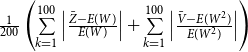 $\frac {1}{200} \left ( \sum \limits _{k=1}^{100} \Big \vert \frac { \bar {Z} - E(W) }{E(W)} \Big \vert + \sum \limits _{k=1}^{100} \Big \vert \frac { \bar {V} - E(W^2) }{E(W^2)} \Big \vert \right )$
. We denote absolute relative bias and its standard deviation as AbsRelBias and SdAbsRelBias, respectively.
$\frac {1}{200} \left ( \sum \limits _{k=1}^{100} \Big \vert \frac { \bar {Z} - E(W) }{E(W)} \Big \vert + \sum \limits _{k=1}^{100} \Big \vert \frac { \bar {V} - E(W^2) }{E(W^2)} \Big \vert \right )$
. We denote absolute relative bias and its standard deviation as AbsRelBias and SdAbsRelBias, respectively.
Table 1 shows that both
 $Z_1$
and
$Z_1$
and
 $\bar {Z}$
are good estimators of
$\bar {Z}$
are good estimators of
 $p$
with the estimator
$p$
with the estimator
 $\bar {Z}$
outperforming the estimator
$\bar {Z}$
outperforming the estimator
 $Z_1$
. The estimator
$Z_1$
. The estimator
 $Z_1$
seems to be a reasonable estimator for
$Z_1$
seems to be a reasonable estimator for
 $p$
when the network is greater than or equal to
$p$
when the network is greater than or equal to
 $N=100$
, but does not perform well when the network size is
$N=100$
, but does not perform well when the network size is
 $10$
.
$10$
.
 $\bar {Z}$
, on the other hand, is a good estimator of
$\bar {Z}$
, on the other hand, is a good estimator of
 $p$
in all cases. These results suggest that
$p$
in all cases. These results suggest that
 $\bar {Z}$
is a more reliable estimator for
$\bar {Z}$
is a more reliable estimator for
 $p$
when working with Model 1, where all edges have a fixed probability
$p$
when working with Model 1, where all edges have a fixed probability
 $p$
.
$p$
.
Absolute relative bias and standard deviations of the proposed estimators
 $Z_1$
and
$Z_1$
and
 $\bar {Z}$
for Model 1 when edge persistence probability is fixed at
$\bar {Z}$
for Model 1 when edge persistence probability is fixed at
 $p = 0.8$

Tables 2 and 3 also demonstrate the consistency of the proposed estimators for large networks. As expected, with more information in hand,
 $\bar {Z}$
also outperforms to the estimator
$\bar {Z}$
also outperforms to the estimator
 $Z_1$
as the number of time steps
$Z_1$
as the number of time steps
 $T$
increases. For a small network size of
$T$
increases. For a small network size of
 $N=10$
,
$N=10$
,
 $Z_1$
does a poor job while the estimator
$Z_1$
does a poor job while the estimator
 $\bar {Z}$
improves as the number of time steps increases from
$\bar {Z}$
improves as the number of time steps increases from
 $T=30$
to
$T=30$
to
 $T=100$
. As the network size increases, both estimators become more reliable and tend to concentrate at the underlying true value of the generating distribution.
$T=100$
. As the network size increases, both estimators become more reliable and tend to concentrate at the underlying true value of the generating distribution.
Absolute relative bias and standard deviations of the proposed estimators
 $Z_1$
and
$Z_1$
and
 $\bar {Z}$
for Model 2 when edge persistence probabilities
$\bar {Z}$
for Model 2 when edge persistence probabilities
 $p_{ij}$
are drawn from
$p_{ij}$
are drawn from
 $\text{Beta}(1,4)$

Absolute relative bias and standard deviations of the proposed estimators
 $Z_1$
and
$Z_1$
and
 $\bar {Z}$
for Model 3 when edge persistence probabilities are modeled as
$\bar {Z}$
for Model 3 when edge persistence probabilities are modeled as
 $p_{ij} = p_{i}p_{j}$
with
$p_{ij} = p_{i}p_{j}$
with
 $p_{i}$
drawn from
$p_{i}$
drawn from
 $\text{Beta}(1,4)$
, for
$\text{Beta}(1,4)$
, for
 $i=1,\cdots ,N$

4. Theoretical results from an infectious disease application
In this section, we demonstrate how the proposed model, despite its simplicity, can offer interesting insights, potentially opening new avenues for exploring theoretical properties in the study of spreading processes on temporal networks. While the TCM can be leveraged for any spreading process over a network, here we examine the spread of an infectious disease. With infectious diseases, the contagion propagates through the population via contact between an infected individual and a susceptible individual. Typically, infectious disease modeling is done via a fully mixed model, which assumes that every individual in the population interacts with every other individual with equal probability or rate. However, in the real world, individuals typically have a small circle of contacts with whom they interact repeatedly. This was emphasized during the COVID-19 pandemic when many individuals practiced social distancing, choosing to interact with only a small group of people dubbed their “social bubble” or “pod” (Hambridge et al., Reference Hambridge, Kahn and Onnela2021; Wu et al., Reference Wu, Li, Shen, He, Tang, Zheng, Fang, Li, Cheng and Shi2022). These repeated contacts, or persistent ties, between individuals are well represented by a network structure and often lead to isolation of the contagion within a particular part of the network. However, as the network topology changes, paths to new, uninfected portions of the network can open up. As such, it is critical to account for both persistent ties and changes in network structure over time. An approach that captures both of these phenomena, like our TCM, may offer a more realistic look at how diseases spread through populations.
To model disease spread, we employ compartmental models, a class of models that divides the population into different groups with respect to disease state. These models assign transition rules, allowing individuals to move between different states. Here, we use the susceptible-infectious-recovered (SIR) model, which assumes that individuals obtain perfect immunity once they recover from the disease. Under this model, individual nodes can be in any of three states: susceptible, infectious, and recovered. In the susceptible state, the node has not been infected but could become infected if it came into contact with an infectious node. That is, the node has no immunity to the disease. In the infected state, the node is infectious and can infect others it comes into contact with. Finally, in the recovered state, the node has recovered from the illness and can no longer infect others or be reinfected. With a stochastic model, nodes move through states probabilistically. Due to the discrete nature of our data, we utilize a discrete-time approach wherein events are defined by transition probabilities per unit time, as opposed to the transition rates used in a continuous time framework. A contact between an infectious and a susceptible node will result in a transmission with probability
 $\beta$
. Similarly, at any given time step a node will recover with probability
$\beta$
. Similarly, at any given time step a node will recover with probability
 $\gamma$
. For simplicity, we assume that at each time step, each edge has persistence probability
$\gamma$
. For simplicity, we assume that at each time step, each edge has persistence probability
 $p$
.
$p$
.
Let
 $R_0$
denote the average number of transmissions from the initially infected node and
$R_0$
denote the average number of transmissions from the initially infected node and
 $R_*$
denote the average number of transmissions in the early stages of the epidemic excluding those from the initial infection. For both a static and dynamic network,
$R_*$
denote the average number of transmissions in the early stages of the epidemic excluding those from the initial infection. For both a static and dynamic network,
 $R_0 = \tau \sum _k kp_k$
, where
$R_0 = \tau \sum _k kp_k$
, where
 $\tau$
is the transmission probability for a link between an infected node and a susceptible node and
$\tau$
is the transmission probability for a link between an infected node and a susceptible node and
 $p_k$
is the probability a node has degree
$p_k$
is the probability a node has degree
 $k$
in the CM. For a static network,
$k$
in the CM. For a static network,
 $R_* = \tau \sum _k q_k(k-1)$
, where
$R_* = \tau \sum _k q_k(k-1)$
, where
 $q_k$
is the excess degree distribution of a node with degree
$q_k$
is the excess degree distribution of a node with degree
 $k$
, that is,
$k$
, that is,
 $q _k = kp_k/\sum _k kp_k$
(Volz and Meyers, Reference Volz and Meyers2009).
$q _k = kp_k/\sum _k kp_k$
(Volz and Meyers, Reference Volz and Meyers2009).
Before further discussion of the reproduction number, we recall an important tool in studying disease spread on a network: the probability-generating function (PGF). Suppose the PGF for the degree distribution of the initial CM network is
 $g(x) = \sum _{k} p_k x^k$
, where
$g(x) = \sum _{k} p_k x^k$
, where
 $p_k$
is the probability that a randomly chosen edge has degree
$p_k$
is the probability that a randomly chosen edge has degree
 $k$
. The PGF of the excess degree distribution is
$k$
. The PGF of the excess degree distribution is
 $g_1(x) = \sum _{k} q_{k} x^{k-1}$
, where
$g_1(x) = \sum _{k} q_{k} x^{k-1}$
, where
 $q_{k} = kp_{k}/\sum _{k} k p_k$
. Thus, we have the following relations:
$q_{k} = kp_{k}/\sum _{k} k p_k$
. Thus, we have the following relations:
 \begin{align} g'(1) &= \sum _k kp_k \end{align}
 \begin{align} g''(1) &= \sum _k k(k-1) p_k \end{align}
 \begin{align} g'_1(1) &= \sum _{k} (k-1) q_{k} = \sum _{k} (k-1) kp_k / \sum _{k} k p_k = g''(1)/g'(1). \end{align}
We now examine the reproduction number at the early stage of the SIR spreading process on the TCM; a proof is provided in Appendix G.
Proposition 4.1.
The reproduction number at the early stage of a discrete-time SIR spreading process on the temporal network is given by
 $R_* =\tau [ (1-\gamma )(1-p)/\gamma + (1 - p + \gamma p ) g''(1) /\big ( \gamma g'(1) \big )]$
, where
$R_* =\tau [ (1-\gamma )(1-p)/\gamma + (1 - p + \gamma p ) g''(1) /\big ( \gamma g'(1) \big )]$
, where
 $\tau = \frac {\beta }{1- p(1-\beta )(1- \gamma )}.$
Next, we examine these results under specific degree distributions.
-
• When the degree distribution follows a Poisson distribution with mean
 $\lambda$
,
$p_k = \lambda ^k$
$\exp (-k)/k!$
, its corresponding PGF is
$g(x) = \exp \big (\lambda (x-1)\big )$
. Then
$g'(1) = \lambda$
and
$g''(1) = \lambda ^2$
. Therefore,
$R_* = \tau [ (1-\gamma )(1-p)/\gamma + (1 - p + \gamma p ) \lambda / \gamma ]$
. For
$p= 1$
, this gives us
$R_* = \tau \lambda$
, which agrees with the results derived in Volz and Meyers (Reference Volz and Meyers2009).
$\lambda$
,
$p_k = \lambda ^k$
$\exp (-k)/k!$
, its corresponding PGF is
$g(x) = \exp \big (\lambda (x-1)\big )$
. Then
$g'(1) = \lambda$
and
$g''(1) = \lambda ^2$
. Therefore,
$R_* = \tau [ (1-\gamma )(1-p)/\gamma + (1 - p + \gamma p ) \lambda / \gamma ]$
. For
$p= 1$
, this gives us
$R_* = \tau \lambda$
, which agrees with the results derived in Volz and Meyers (Reference Volz and Meyers2009). -
• When the degree distribution satisfies
$p_k = 1$
, if
$k = M$
for some
$ 1 \leq M \leq N$
where
$N$
is the network size, then the PGF is given by
$g(x) = x^M$
. So
$g''(1)/g'(1) = M-1$
, and therefore
$R_* = \tau [ (1-\gamma )(1-p)/\gamma + (1 - p + \gamma p ) (M-1) / \gamma ]$
. Notice that if
$k=N$
, we have a fully connected network. Under this scenario, the reproduction number is given by
$R_* = \tau$
$[ (1-\gamma )(1-p)/\gamma + (1 - p + \gamma p ) (N-1) / \gamma$
]. For
$p=1$
, this reduces to
$R_* = \tau (N-1)$
.


Additionally, when the temporal network is static over time,
 $p = 1$
. The reproduction number at the early stages is then
$p = 1$
. The reproduction number at the early stages is then
 $R_* = \tau g''(1)/g'(1)$
, which agrees with the
$R_* = \tau g''(1)/g'(1)$
, which agrees with the
 $R_*$
value for a static network introduced above. When the temporal network evolves as independent draws from a CM, then
$R_*$
value for a static network introduced above. When the temporal network evolves as independent draws from a CM, then
 $p=0$
. Under this scenario, the reproduction number at the early stage is
$p=0$
. Under this scenario, the reproduction number at the early stage is
 $R_* = \tau [ (1-\gamma )/\gamma + g''(1) /\big ( \gamma g'(1) \big )] = \beta [ (1-\gamma )/\gamma + g''(1) /\big ( \gamma g'(1) \big )]$
.
$R_* = \tau [ (1-\gamma )/\gamma + g''(1) /\big ( \gamma g'(1) \big )] = \beta [ (1-\gamma )/\gamma + g''(1) /\big ( \gamma g'(1) \big )]$
.
5. Fitting the model to empirical network data
In this section, we show how to use the three proposed TCMs to fit empirical network data and examine the fit of the generated temporal networks. The empirical data in this study was collected by the Copenhagen Network Study data and is publicly available (Sapiezynski et al., Reference Sapiezynski, Stopczynski, Lassen and Lehmann2019). This data set contains information about the connectivity patterns of 706 students at the Technical University of Denmark over 28 days in February 2014. During the study period, participants agreed to use loaner cell phones from researchers as their primary phones. The proximity patterns were collected using Bluetooth where the approximate pairwise distances of phones were obtained using the received signal strength indicator (RSSI) every five minutes. We assigned a connection between two persons if there was at least one strong Bluetooth ping with RSSI
 $\geq -\text{75dBm}$
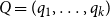
(Hambridge et al., Reference Hambridge, Kahn and Onnela2021). Because the empirical data reflects student proximity patterns, they fluctuate significantly on a daily basis. Students were more likely to connect during the week if they were in the same class, but on weekends, their proximity patterns were likely driven by their personal contact networks. Our models cannot capture the weekday–weekend variability because they require a comparable number of edges at each time instance. Therefore, we further processed the daily network data by combining each of the seven daily networks into a single weekly network. In particular, we established a weekly network by taking the union of the daily networks of each weekly batch of 7 daily networks. As a result, the period of 28 days yielded 4 weekly networks, denoted as
$\geq -\text{75dBm}$
(Hambridge et al., Reference Hambridge, Kahn and Onnela2021). Because the empirical data reflects student proximity patterns, they fluctuate significantly on a daily basis. Students were more likely to connect during the week if they were in the same class, but on weekends, their proximity patterns were likely driven by their personal contact networks. Our models cannot capture the weekday–weekend variability because they require a comparable number of edges at each time instance. Therefore, we further processed the daily network data by combining each of the seven daily networks into a single weekly network. In particular, we established a weekly network by taking the union of the daily networks of each weekly batch of 7 daily networks. As a result, the period of 28 days yielded 4 weekly networks, denoted as
 $\{ G_1, G_2, G_3, G_4\}$
. Figure 2 shows their degree distributions.
$\{ G_1, G_2, G_3, G_4\}$
. Figure 2 shows their degree distributions.
Degree distributions of weekly empirical networks
 $G_1, G_2, G_3, G_4$
.
$G_1, G_2, G_3, G_4$
.

To fit the TCM models, we used
 $G_1$
as the starting point and counted the number of edges in
$G_1$
as the starting point and counted the number of edges in
 $G_1$
that were retained in
$G_1$
that were retained in
 $G_2$
and
$G_2$
and
 $G_3$
. For Model 1, we calculated the fixed edge persistence rate as the ratio of the number of edges in
$G_3$
. For Model 1, we calculated the fixed edge persistence rate as the ratio of the number of edges in
 $G_1$
that persisted into
$G_1$
that persisted into
 $G_2$
. For Models 2 and 3, we assumed that the edge-level and node-level persistence rates were generated from Beta distributions. The first and second moments of these Beta distributions were estimated by the ratios of the number of edges in
$G_2$
. For Models 2 and 3, we assumed that the edge-level and node-level persistence rates were generated from Beta distributions. The first and second moments of these Beta distributions were estimated by the ratios of the number of edges in
 $G_1$
that persisted into
$G_1$
that persisted into
 $G_2$
and
$G_2$
and
 $G_3$
, respectively. Using the estimated first two moments, we determined the shape and scale parameters of the Beta distributions. The empirical weekly data gave us the estimate
$G_3$
, respectively. Using the estimated first two moments, we determined the shape and scale parameters of the Beta distributions. The empirical weekly data gave us the estimate
 $\hat {p} = 0.476$
for Model 1; the Beta distributions for Models 2 and 3 were estimated as Beta
$\hat {p} = 0.476$
for Model 1; the Beta distributions for Models 2 and 3 were estimated as Beta
 $(0.975, 1.074)$
and Beta
$(0.975, 1.074)$
and Beta
 $(1.171, 1.562)$
, respectively. With the estimated model parameters, we used
$(1.171, 1.562)$
, respectively. With the estimated model parameters, we used
 $G_1$
as the initial network and used the TCM models to obtain predicted networks
$G_1$
as the initial network and used the TCM models to obtain predicted networks
 $\hat {G}_2^{(M_k)}, \hat {G}_3^{(M_k)},\hat {G}_4^{(M_k)}$
for the empirical networks
$\hat {G}_2^{(M_k)}, \hat {G}_3^{(M_k)},\hat {G}_4^{(M_k)}$
for the empirical networks
 $G_2, G_3, G_4$
, respectively. Here
$G_2, G_3, G_4$
, respectively. Here
 $k = 1, 2, 3$
represents Models 1–3, respectively. As a benchmark, we employed the naive TCM, in which all edges were broken and rewired randomly at each time step. We refer to this CM as Model A. Furthermore, we also compare the proposed models with the dynamic random graphs with arbitrary expected degrees in Zhang et al. (2017). In this model, at each time step, new edges between each node pair
$k = 1, 2, 3$
represents Models 1–3, respectively. As a benchmark, we employed the naive TCM, in which all edges were broken and rewired randomly at each time step. We refer to this CM as Model A. Furthermore, we also compare the proposed models with the dynamic random graphs with arbitrary expected degrees in Zhang et al. (2017). In this model, at each time step, new edges between each node pair
 $i, j$
at is added with probability
$i, j$
at is added with probability
 $1-e^{-\lambda _{i j}}$
and removing existing edges at with probability
$1-e^{-\lambda _{i j}}$
and removing existing edges at with probability
 $1-e^{-\mu }$
, where
$1-e^{-\mu }$
, where
 $\lambda _{i j}=\mu d_i d_j / 2 m$
,
$\lambda _{i j}=\mu d_i d_j / 2 m$
,
 $m=\frac {1}{2} \sum _i d_i$
,
$m=\frac {1}{2} \sum _i d_i$
,
 $d_i$
is degree of node
$d_i$
is degree of node
 $i$
(Refer to Zhang et al., (Reference Zhang, Moore and Newman2017) for more details). We denote this model as Model B.
$i$
(Refer to Zhang et al., (Reference Zhang, Moore and Newman2017) for more details). We denote this model as Model B.
To assess the performance of the TCM models, we compared the distances between the degree distributions of networks generated with Model A, Model B, Models 1–3 with the empirical networks
 $G_2, G_3, G_4$
. We denote the distances between the model-based networks
$G_2, G_3, G_4$
. We denote the distances between the model-based networks
 $\hat {G}_2^{(M_k)}$
,
$\hat {G}_2^{(M_k)}$
,
 $\hat {G}_3^{(M_k)}$
,
$\hat {G}_3^{(M_k)}$
,
 $\hat {G}_4^{(M_k)}$
and the corresponding empirical networks
$\hat {G}_4^{(M_k)}$
and the corresponding empirical networks
 $G_2, G_3, G_4$
as
$G_2, G_3, G_4$
as
 $D_2^{(M_k)}, D_3^{(M_k)}, D_4^{(M_k)}$
. We computed the average distances
$D_2^{(M_k)}, D_3^{(M_k)}, D_4^{(M_k)}$
. We computed the average distances
 $\bar {D}^{(M_k)} = \frac {1}{3}\left (D_2^{(M_k)} + D_3^{(M_k)} + D_4^{(M_k)}\right )$
to assess the performance of the models. We calculated the means and standard deviations of
$\bar {D}^{(M_k)} = \frac {1}{3}\left (D_2^{(M_k)} + D_3^{(M_k)} + D_4^{(M_k)}\right )$
to assess the performance of the models. We calculated the means and standard deviations of
 $\bar {D}^{(M_k)}$
from 100 simulation runs and used them as final goodness-of-fit metrics to assess the performance of the models. In particular, for run
$\bar {D}^{(M_k)}$
from 100 simulation runs and used them as final goodness-of-fit metrics to assess the performance of the models. In particular, for run
 $i$
, we calculated the average distances
$i$
, we calculated the average distances
 $\bar {D}^{(M_k,i)}$
; the final metrics for comparing the four models are the means and standard deviations of these metrics. The distances considered include the total variation distance,
$\bar {D}^{(M_k,i)}$
; the final metrics for comparing the four models are the means and standard deviations of these metrics. The distances considered include the total variation distance,
 $ D_T = \frac {1}{2} \sum _{i=1}^k |p_i - q_i|$
; the Jaccard edge similarity,
$ D_T = \frac {1}{2} \sum _{i=1}^k |p_i - q_i|$
; the Jaccard edge similarity,
 $ D_J$
which is equal to the ratio of shared edges between
$ D_J$
which is equal to the ratio of shared edges between
 $G$
and
$G$
and
 $\hat {G}$
to the total number of unique edges in
$\hat {G}$
to the total number of unique edges in
 $G$
and
$G$
and
 $\hat {G}$
; and the absolute difference in average clustering coefficient,
$\hat {G}$
; and the absolute difference in average clustering coefficient,
 $ D_{\text{cl}} = \vert C_G - C_{\hat {G}} \vert$
. Here,
$ D_{\text{cl}} = \vert C_G - C_{\hat {G}} \vert$
. Here,
 $ P = (p_1, \ldots , p_k)$
and
$ P = (p_1, \ldots , p_k)$
and
 $ Q = (q_1, \ldots , q_k)$
denote the discrete degree distributions of the empirical network
$ Q = (q_1, \ldots , q_k)$
denote the discrete degree distributions of the empirical network
 $G$
and the model-based network
$G$
and the model-based network
 $\hat {G}$
, respectively, while
$\hat {G}$
, respectively, while
 $ C_G$
and
$ C_G$
and
 $ C_{\hat {G}}$
are their corresponding average clustering coefficients. For total variation and average clustering difference, smaller distance values indicate that the model-based networks more closely resemble the empirical networks, suggesting a better model fit. In contrast, a higher Jaccard edge similarity value indicates a better fit.
$ C_{\hat {G}}$
are their corresponding average clustering coefficients. For total variation and average clustering difference, smaller distance values indicate that the model-based networks more closely resemble the empirical networks, suggesting a better model fit. In contrast, a higher Jaccard edge similarity value indicates a better fit.
Table 4 shows that Models 2, 3, and B yield the best fit to the empirical data. In general, the performance of Models 2 and 3 is comparable to that of Model B. While Model B outperforms Models 2 and 3 in terms of total variation distance, Models 2 and 3 achieve better performance than Model B with respect to the average clustering difference and Jaccard edge similarity. It is important to note that estimating Model B requires more detailed information than Models 2 and 3. Specifically, while Models 2 and 3 only require knowledge of the number of edges remaining after one and two time steps, Model B requires tracking edges status that emerge, dissolve, or remain unchanged during the first two time steps. Model 1 performed worse than Models 2 and 3, and Model A had the worst performance. The results demonstrate that model fit generally improves from Model 1 to Model 2 to Model 3. The improvement in model fit was to be expected because Model A uses data about the initial network only; Model 1 requires additional knowledge of the number of edges that remain in the initial network
 $G_1$
after one time step, and Models 2 and 3 require knowledge of the number of edges that remain after one and two time steps.
$G_1$
after one time step, and Models 2 and 3 require knowledge of the number of edges that remain after one and two time steps.
Assessment of model goodness-of-fit using means and standard deviations of total variation distance between degree distributions, Jaccard edge similarity, and absolute difference in average clustering coefficients over 100 runs

To further evaluate the robustness of the proposed model, we repeated the procedure using student contact patterns from five weekdays only in the Copenhagen Network Study. The results, shown in Table 5, are consistent with those in Table 4, which was based on data from all seven days of the week. This consistency of the results suggests that the model is able to capture temporal contact patterns in social interaction networks.
Assessment of model goodness-of-fit using means and standard deviations of total variation distance between degree distributions, Jaccard edge similarity, and absolute difference in average clustering coefficients over 100 runs for five weekday networks

6. Discussion and conclusion
We introduced the TCM, a family of generative models for a temporal network, as well as approaches for estimating model parameters. The proposed generative model is simple and flexible. The modeling framework allows the edge persistence probability to be fixed, generated from a distribution, or constructed from the corresponding node-level persistence probabilities. Our simulation studies showed that our estimators have good statistical properties. We then presented a theoretical application of the proposed model to the spread of an infectious disease and demonstrated how to fit the model to empirical data from the Copenhagen Network Study.
We proposed consistent estimators for the model parameters and provided the convergence rate of the proposed estimators. We additionally showed that, when the persistence probability is constant across edges, using the network evolution process can give us a more precise estimator with a faster convergence rate. However, when persistence probabilities are generated at random or are the product of the node-level persistence probabilities, care must be taken when using an estimator that relies on averages over the entire course of the network’s evolution. Instead, it might be advantageous to consider alternative modeling strategies, such as those in which persistence probabilities are periodically updated. If additional information on this time interval is available, then a design that incorporates the network evolution process will give us a finer estimator with an accelerated convergence rate. This finding addresses a key question regarding the level of temporal resolution needed for reliable estimation in dynamic network settings: the resolution depends strongly on the nature of the underlying temporal process. For the proposed class of temporal networks, the only data required for consistent estimation are the counts of edges that persist up to
 $ k$
time steps from the original network, where
$ k$
time steps from the original network, where
 $ k$
corresponds to the highest-order moment of the generating distribution. This insight reduces the effort involved in data collection and storage for temporal networks governed by the TCM.
$ k$
corresponds to the highest-order moment of the generating distribution. This insight reduces the effort involved in data collection and storage for temporal networks governed by the TCM.
Additionally, we highlighted the merits of TCM through both a theoretical application to the study of spreading processes on temporal networks and an empirical data analysis. In the theoretical setting, we examined an SIR spreading model on a temporal network under the assumption of constant edge persistence probability and derived an explicit formula for the reproduction number during the early stage of the epidemic. In the empirical analysis, TCM demonstrated good fit with real-world temporal network data.
Further research directions might involve examining a good estimator for the periodic information in Models 2 and 3, extending the temporal model to include network size growth information, and investigating various epidemic characteristics of spreading processes on the temporal network of the three models. All of these potential developments, as well as the broad range of applications for temporal networks, offer an exciting future for the study of time-varying networks (Holme, Reference Holme2015; Jordan et al., Reference Jordan, Winer and Salem2020; Hosseinzadeh et al., Reference Hosseinzadeh, Cannataro, Guzzi and Dondi2022). With technological advances, particularly Bluetooth technology, network data is becoming more accessible than ever. How we can appropriately employ these new datasets for public health insights is an interesting subject that requires further research. We believe that statistical techniques with robust theoretical underpinnings are the foundation for leveraging the vast amounts of data available for the common good.
An important contribution of the TCM is that it provides a principled solution to the problem of temporal granularity in network analysis. Prior work has shown that the resolution at which interactions are observed can substantially alter conclusions about spreading dynamics, robustness, and network structure (Holme and Saramäki, Reference Holme and Saramäki2012; Holme, Reference Holme2015). If data are aggregated too coarsely, essential ordering and persistence effects are lost; if collected at overly fine resolution, data can be noisy, costly, and difficult to obtain (Vanhems et al., Reference Vanhems, Barrat, Cattuto, Pinton, Khanafer, Régis, Kim, Comte and Voirin2013; Sapiezynski et al., Reference Sapiezynski, Stopczynski, Lassen and Lehmann2019). Despite this recognition, a rigorous statistical characterization of how much temporal information is sufficient has been lacking. Our results show that for the class of TCMs, consistent inference requires only edge persistence counts up to a finite horizon of length
 $k$
, thereby providing a tractable statistical solution to this problem for this model class.
$k$
, thereby providing a tractable statistical solution to this problem for this model class.
Our modeling framework is relevant in application domains where persistence and temporal resolution are essential. For example, within network biology, distinguishing stable from transient protein interactions (Barabasi and Oltvai, Reference Barabasi and Oltvai2004) can be framed through persistence-based inference. In human mobility, separating recurrent commuting flows from irregular trips (Barbosa et al., Reference Barbosa, Barthelemy, Ghoshal, James, Lenormand, Louail and Tomasini2018) can benefit from a principled treatment of temporal resolution. In studies of bursty human dynamics, persistence parameters can provide a way to capture stability amid temporal clustering (Karsai et al., Reference Karsai, Jo and Kimmo2018). In financial networks, where aggregation can obscure underlying creditor–debtor structures (Barucca and Lillo, Reference Barucca and Lillo2016), the TCM can help track the evolving backbone of interbank relationships. The framework can also be applied to study changes in resource access in interpersonal networks, assessing growth in interorganizational partnerships, comparing persistence across communities, and analyzing the interplay between relational states and relational events. By formalizing persistence within a statistical framework, the TCM provides theoretical clarity and practical insights for temporal network research.
Funding statement
H.H. was supported by a Harvard University Department of Biostatistics scholarship and a U.S. Government scholarship. T.M.L and J.P.O. were supported by a National Institutes of Health award (NIAID R01 AI138901). The funding sources had no role in study design, data analysis, data interpretation, or the writing of the paper.
Competing interests
None.
Data availability statement
The empirical network data is publicly available at The Copenhagen Networks Study interaction data Sapiezynski et al. (Reference Sapiezynski, Stopczynski, Lassen and Lehmann2019). Python code used in this study is publicly available at https://github.com/onnela-lab/temporal-configuration-model.
Appendix A. Proof of Lemma 2.1
Proof.
We have
 $Z_{1}=X_{1}/X_{0} = \sum _{(i,j) \in G_0} \text{Bernoulli}(p)/ X_{0}$
. Since
$Z_{1}=X_{1}/X_{0} = \sum _{(i,j) \in G_0} \text{Bernoulli}(p)/ X_{0}$
. Since
 $\sum _{(i,j) \in G_0} \text{Bernoulli}(p)$
is the sum of independent Bernoulli random variables, applying the central limit theorem we have
$\sum _{(i,j) \in G_0} \text{Bernoulli}(p)$
is the sum of independent Bernoulli random variables, applying the central limit theorem we have
 $\frac {Z_1 -p}{\sqrt {\big ( p(1-p)\big )/X_0}}$
converges to a standard normal distribution as
$\frac {Z_1 -p}{\sqrt {\big ( p(1-p)\big )/X_0}}$
converges to a standard normal distribution as
 $X_0 \rightarrow \infty .$
Thus,
 $Z_1$
is an unbiased and consistent estimator for
$Z_1$
is an unbiased and consistent estimator for
 $p$
.
$p$
.
Appendix B. Proof of Theorem 2.2
Proof.
It follows from Lemma 2.1 that each estimator
 $Z_k$
is an unbiased and consistent estimator for the persistence probability
$Z_k$
is an unbiased and consistent estimator for the persistence probability
 $p$
, for all
$p$
, for all
 $k = 1,\cdots ,T$
. Therefore,
$k = 1,\cdots ,T$
. Therefore,
 $\bar {Z} =\frac {1}{T}\, \sum _{i=1}^{T}Z_{i}$
is also an unbiased and consistent estimator of
$\bar {Z} =\frac {1}{T}\, \sum _{i=1}^{T}Z_{i}$
is also an unbiased and consistent estimator of
 $p$
.
$p$
.
Denote
 $S_{T}=\sum _{i=1}^{T}Z_{i}$
and
$S_{T}=\sum _{i=1}^{T}Z_{i}$
and
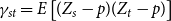 $\gamma _{st}=E\left [(Z_{s}-p)(Z_{t}-p)\right ]$
for all
$\gamma _{st}=E\left [(Z_{s}-p)(Z_{t}-p)\right ]$
for all
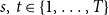 $s,\,t\in \{1,\ldots ,T\}$
. We now evaluate the variance of
$s,\,t\in \{1,\ldots ,T\}$
. We now evaluate the variance of
 $S_{T}$
.
$S_{T}$
.
 \begin{align*} \text{Var}(S_{T})&=E\left [(S_{T}-pT)^{2}\right ] =E\left [\left (\sum _{i=1}^{T}Z_{i}-pT\right)^{\!\!2}\right ] =\sum _{s=1}^{T}\sum _{t=1}^{T}E\left [(Z_{s}-p)(Z_{t}-p)\right ]= \sum _{s=1}^{T}\sum _{t=1}^{T}\gamma _{st}. \end{align*}
For any
 $s\gt t$
, we have
$s\gt t$
, we have
 \begin{align*} \gamma _{st}&=E\left [(Z_{s}-p)(Z_{t}-p)\right ] = E(Z_{s}Z_{t})-p\,E(Z_{s})-p\,E(Z_{t})+p^{2} =E(Z_{s}Z_{t})-p^{2}-p^{2}+p^{2}\\ &=E\left (\frac {X_{s}}{X_{s-1}^{+}}\,\frac {X_{t}}{X_{t-1}^{+}}\right )-p^{2} =E\left [E\left (\frac {X_{s}}{X_{s-1}^{+}}\,\frac {X_{t}}{X_{t-1}^{+}}\Big | X_{s-1}^{+}\right )\right ]-p^{2} \\ &=E\left [E\left (\frac {X_{s}}{X_{s-1}^{+}}\Big | X_{s-1}^{+}\right )\right ]E\left (\frac {X_{t}}{X_{t-1}^{+}}\right )-p^{2} \ \ \ \text{by independence of $\frac {X_{t}}{X_{t-1}^{+}}$ and $E\left (\frac {X_{s}}{X_{s-1}^{+}}\Big | X_{s-1}^{+}\right )$}\\ &=p\,E\left (\frac {X_{t}}{X_{t-1}^{+}}\right )-p^{2}=p^{2}-p^{2} = 0. \end{align*}
Thus,
 $\gamma _{st}=0$
for any
$\gamma _{st}=0$
for any
 $s\gt t$
. Similarly,
$s\gt t$
. Similarly,
 $\gamma _{st}=0$
for any
$\gamma _{st}=0$
for any
 $s\lt t$
. Therefore,
$s\lt t$
. Therefore,
 $\text{Var}(S_{T}) = \sum _{s=1}^{T}\sum _{t=1}^{T}\gamma _{st} = \sum _{s=1}^{T}\gamma _{ss}$
.
$\text{Var}(S_{T}) = \sum _{s=1}^{T}\sum _{t=1}^{T}\gamma _{st} = \sum _{s=1}^{T}\gamma _{ss}$
.
For
 $T = o(X_0)$
, we have
$T = o(X_0)$
, we have
 $X_{s-1}^{+} = X_0 + o(1)$
, for all
$X_{s-1}^{+} = X_0 + o(1)$
, for all
 $s \in 1,\cdots , T$
. Therefore,
$s \in 1,\cdots , T$
. Therefore,
 \begin{align*} \gamma _{ss} &=E\big ( (Z_{s}-p)(Z_{s}-p)\big ) =E(Z_{s}^{2})-p^2 =E\left [\left (\frac {X_{s}}{X_{s-1}^{+}}\right)^{\!\!2}\right ] - p^2\\ &=E\left [E\left (\left (\frac {X_{s}}{X_{s-1}^{+}}\right)^{\!\!2}\Big |X_{s-1}^{+}\right )\right ] - p^2 = E\left [\left (\frac {1}{X_{s-1}^{+}}\right)^{\!\!2} E\left (X_{s}^{2}\Big |X_{s-1}^{+}\right )\right ] - p^2 \\ &= E\left [\left (\frac {1}{X_{s-1}^{+}}\right )^{\!\!2} \left [X_{s-1}^{+}\,p\,(1-p)+(p\,X_{s-1}^{+})^{2}\right ]\right ] - p^2 \\ & = E\left [\frac {p\,(1-p)}{X_{s-1}^{+}}\right ] \leq \frac {C_1}{X_0}, \quad \text{for some}\ C_1 \gt 0. \end{align*}
This gives us
 $\text{Var}(S_{T}) = \sum _{s=1}^{T}\gamma _{ss} \leq T \frac {C_1}{X_0}$
. Applying the Chebyshev’s, for some
$\text{Var}(S_{T}) = \sum _{s=1}^{T}\gamma _{ss} \leq T \frac {C_1}{X_0}$
. Applying the Chebyshev’s, for some
 $C_2\gt 0$
and
$C_2\gt 0$
and
 $0\lt \delta \lt 1/2$
, we have
$0\lt \delta \lt 1/2$
, we have
 \begin{align*} P\left (\left |\bar {Z}-p\right |\geq C_2 \sqrt {\frac {1}{X_0}} \left (\frac {1}{T}\right )^{1/2-\delta }\right )&\leq \frac {E\left [(\bar {Z}-p)^{2}\right ]}{C_2^2 \frac {1}{X_0} (\frac {1}{T})^{1-2\delta }}=\frac {E\left [(S_{T}-T\,p)^{2}\right ]}{T^{2}C_2^2 \frac {1}{X_0} (\frac {1}{T})^{1-2\delta }}\\ &\leq \frac {T \frac {C_1}{X_0}}{T^{2}C_2^2 \frac {1}{X_0} (\frac {1}{T})^{1-2\delta }}= \frac {C_1}{C_2^2 T^{2\delta }}\rightarrow 0. \end{align*}
Thus,
 $ \bar {Z}$
converges to
$ \bar {Z}$
converges to
 $p$
at the rate of
$p$
at the rate of
 $O_p\left (\sqrt {\frac {1}{X_0}} (\frac {1}{T})^{1/2-\delta }\right )$
.
$O_p\left (\sqrt {\frac {1}{X_0}} (\frac {1}{T})^{1/2-\delta }\right )$
.
Appendix C. Proof of Lemma 2.3
Proof.
We first prove that, for any given combination of edge persistence probabilities drawn from
 $W$
,
$W$
,
 $Z_1$
is an unbiased and consistent estimator for the average of the edge persistence probabilities. We have
$Z_1$
is an unbiased and consistent estimator for the average of the edge persistence probabilities. We have
 $Z_{1}=X_{1}/X_{0} = \sum _{(i,j) \in G_0} \text{Bernoulli}(p_{ij})/ X_{0}$
, where
$Z_{1}=X_{1}/X_{0} = \sum _{(i,j) \in G_0} \text{Bernoulli}(p_{ij})/ X_{0}$
, where
 $\text{Bernoulli}(p_{ij})$
are independent variables. For simplicity, let us re-enumerate the sequence of independent
$\text{Bernoulli}(p_{ij})$
are independent variables. For simplicity, let us re-enumerate the sequence of independent
 $\text{Bernoulli}(p_{ij})$
for all
$\text{Bernoulli}(p_{ij})$
for all
 $(i,j) \in G_0$
and denote them as
$(i,j) \in G_0$
and denote them as
 $U_1, U_2, \cdots , U_{X_0}$
, where
$U_1, U_2, \cdots , U_{X_0}$
, where
 $U_i \sim \text{Bernoulli}(p_i)$
for
$U_i \sim \text{Bernoulli}(p_i)$
for
 $i=1,\cdots ,X_0$
. Then
$i=1,\cdots ,X_0$
. Then
 $Z_1 = \frac {1}{X_0} \sum _{i=1}^{X_0}U_i$
. Denote
$Z_1 = \frac {1}{X_0} \sum _{i=1}^{X_0}U_i$
. Denote
 $\mu _{X_0} = \frac {1}{X_0} \sum _{i=1}^{X_0}p_i$
and
$\mu _{X_0} = \frac {1}{X_0} \sum _{i=1}^{X_0}p_i$
and
 $\sigma _{X_0} = \frac {1}{X_0} \sqrt {\sum _{i=1}^{X_0}p_i(1-p_i)}$
.
$\sigma _{X_0} = \frac {1}{X_0} \sqrt {\sum _{i=1}^{X_0}p_i(1-p_i)}$
.
Using the Lyapunov central limit theorem for independent non-identical distributions, we see that
 $(Z_1 - \mu _{X_0})/\sigma _{X_0}$
will converge to a standard normal distribution if we can verify the Lyapunov condition (C1) below:
$(Z_1 - \mu _{X_0})/\sigma _{X_0}$
will converge to a standard normal distribution if we can verify the Lyapunov condition (C1) below:
 \begin{equation} \lim _{X_0 \rightarrow \infty }\frac {1}{\sigma _{X_0}^{\!\!2+\delta }} \sum _{i=1}^{X_0} \left (\frac {1}{X_0}\right )^{\!\!2+\delta }E\left \vert U_i - p_i\right \vert ^{2+\delta } \rightarrow 0, \text{for some} \ \delta \gt 0. \end{equation}
Since
 $0 \leq p_i \leq 1$
for all
$0 \leq p_i \leq 1$
for all
 $i$
,
$i$
,
 $\sum _{i=1}^{X_0}p_i(1-p_i)$
is of the same order as
$\sum _{i=1}^{X_0}p_i(1-p_i)$
is of the same order as
 $\sum _{i=1}^{X_0}p_i$
. Therefore,
$\sum _{i=1}^{X_0}p_i$
. Therefore,
 $\sum _{i=1}^{X_0}p_i(1-p_i) \rightarrow \infty$
as
$\sum _{i=1}^{X_0}p_i(1-p_i) \rightarrow \infty$
as
 $X_0 \rightarrow \infty$
. In addition, we also have
$X_0 \rightarrow \infty$
. In addition, we also have
 \begin{align*} E\vert U_i - p_i\vert ^{2+\delta } &= p_i (1 - p_i)^{2+\delta } + (1-p_i)p_i^{2+\delta } \\ &\leq p_i(1-p_i)^2 + (1-p_i)p_i^2 = p_i(1-p_i). \end{align*}
Therefore,
 \begin{align*} \lim _{X_0 \rightarrow \infty }\frac {1}{\sigma _{X_0}^{2+\delta }} \sum _{i=1}^{X_0} \left (\frac {1}{X_0}\right)^{\!2+\delta }E\left \vert U_i - p_i\right \vert ^{2+\delta } &= \lim _{X_0 \rightarrow \infty }\frac {1}{\big ( \sum _{i=1}^{X_0}p_i(1-p_i) \big ) ^{1+\delta /2}} \sum _{i=1}^{X_0}E\vert U_i - p_i\vert ^{2+\delta }\\ &\leq \lim _{X_0 \rightarrow \infty }\frac {\sum _{i=1}^{X_0}p_i(1-p_i)}{\big ( \sum _{i=1}^{X_0}p_i(1-p_i) \big ) ^{1+\delta /2}} \\ &= \lim _{X_0 \rightarrow \infty }\frac {1}{\big ( \sum _{i=1}^{X_0}p_i(1-p_i) \big ) ^{\delta /2}} \rightarrow 0.\\ \end{align*}
So,
 $\frac {Z_1 - \mu _{X_0}}{\sigma _{X_0}}$
converges to a standard normal distribution, as
$\frac {Z_1 - \mu _{X_0}}{\sigma _{X_0}}$
converges to a standard normal distribution, as
 $X_0 \rightarrow \infty$
.
$X_0 \rightarrow \infty$
.
The central limit theorem for random observations generated from distribution
 $W$
gives us
$W$
gives us
 $\mu _{X_0} = E(W) + O_p\left (\sqrt {\frac {1}{X_0}}\right )$
. Furthermore, we also have that
$\mu _{X_0} = E(W) + O_p\left (\sqrt {\frac {1}{X_0}}\right )$
. Furthermore, we also have that
 $E(Z_1) = E( \frac {1}{X_0} \sum _{i=1}^{X_0}p_i) = E(W)$
. Therefore,
$E(Z_1) = E( \frac {1}{X_0} \sum _{i=1}^{X_0}p_i) = E(W)$
. Therefore,
 $Z_1$
is an unbiased and consistent estimator of the first moment
$Z_1$
is an unbiased and consistent estimator of the first moment
 $E(W)$
of distribution
$E(W)$
of distribution
 $W$
as
$W$
as
 $X_0 \rightarrow \infty$
.
$X_0 \rightarrow \infty$
.
Appendix D. Proof of Theorem 2.4
Proof.
It follows from Lemma 2.3 that each
 $Z_k$
is an unbiased and consistent estimator for the first moment
$Z_k$
is an unbiased and consistent estimator for the first moment
 $E(W)$
, for
$E(W)$
, for
 $k = 1,\cdots ,m$
. Then
$k = 1,\cdots ,m$
. Then
 $E(\bar {Z}) = E\left (\sum _{k=1}^{m} Z_k/m\right ) = E(W).$
In other words,
$E(\bar {Z}) = E\left (\sum _{k=1}^{m} Z_k/m\right ) = E(W).$
In other words,
 $\bar {Z}$
is also an unbiased and consistent estimator for
$\bar {Z}$
is also an unbiased and consistent estimator for
 $E(W)$
, as
$E(W)$
, as
 $X_0, X_{T_0}, \cdots , X_{mT_0} \rightarrow \infty$
.
$X_0, X_{T_0}, \cdots , X_{mT_0} \rightarrow \infty$
.
To obtain the convergence rate of
 $\bar {Z}$
, we first provide the upper bound for
$\bar {Z}$
, we first provide the upper bound for
 $E\big (\sum _{s=1}^{m} Z_s - m\,E(W)\big )^{2}$
:
$E\big (\sum _{s=1}^{m} Z_s - m\,E(W)\big )^{2}$
:
 \begin{align*} E\left (\sum _{s=1}^m Z_s - m\,E(W)\right )^{\!\!2} &= \text{Var}\left (\sum _{s=1}^{m} Z_s - m\,E(W)\right ) = \text{Var} \left ( \sum _{s=1}^{m} Z_s \right ) \\ & = \sum _{s=1}^{m} \text{Var} (Z_s) + 2 \sum _{s\gt t; s, t =1}^{m} \text{Cov} ( Z_s , Z_t ) . \end{align*}
For any
 $s\gt t$
, we have
$s\gt t$
, we have
 \begin{align*} \text{Cov} ( Z_s , Z_t ) & =E\left (\frac {X_{(s-1)T_0+1}}{X_{(s-1)T_0}^{+}}\cdot \frac {X_{(t-1)T_0+1}}{X_{(t-1)T_0}^{+}}\right ) - \big ( E(W) \big )^2 \\ &=E\left [E\left (\frac {X_{(s-1)T_0+1}}{X_{(s-1)T_0}^{+}}\cdot \frac {X_{(t-1)T_0+1}}{X_{(t-1)T_0}^{+}}\Bigg | \mathcal{F}_{(s-1)T_0}^{+}\right )\right ] - \big ( E(W) \big )^2 \\ &=E\left [E\left (\frac {X_{(s-1)T_0+1}}{X_{(s-1)T_0}^{+}}\Bigg | \mathcal{F}_{(s-1)T_0}^{+}\right )\right ] E\left ( \frac {X_{(t-1)T_0+1}}{X_{(t-1)T_0}^{+}} \right ) - \big ( E(W) \big )^2 \\ &= E(W) E(W) - \big ( E(W) \big )^2 = 0. \end{align*}
In addition,
 \begin{align*} \text{Var} ( Z_s ) &= E\left [\left (\frac {X_{(s-1)T_0+1}}{X_{(s-1)T_0}^{+}}\right)^{\!\!2}\right ] - \big ( E(W) \big )^2 = E\left [E\left (\left (\frac {X_{(s-1)T_0+1}}{X_{(s-1)T_0}^{+}}\right )^{\!\!2} \Bigg | \mathcal{F}_{(s-1)T_0}^{+} \right )\right ] - \big ( E(W) \big )^2\\ &= E\left [ \left ( \frac {1}{X_{(s-1)T_0}^{+}} \right)^{\!\!2} E \left ( X_{(s-1)T_0+1}^2 \Bigg | \mathcal{F}_{(s-1)T_0}^{+} \right ) \right ] - \big ( E(W) \big )^2.\\ \end{align*}
Since
 $X_{(s-1)T_0+1}$
is the summation of independent Bernoulli variables
$X_{(s-1)T_0+1}$
is the summation of independent Bernoulli variables
 $\text{Bernoulli}\left (p_{ij}^{(s)}\right )$
, where
$\text{Bernoulli}\left (p_{ij}^{(s)}\right )$
, where
 $(i,j)\in \boldsymbol{A}_{(s-1)T_0}^+$
, we have
$(i,j)\in \boldsymbol{A}_{(s-1)T_0}^+$
, we have
 \begin{align*} E \left ( X_{(s-1)T_0+1}^2 \Big | \mathcal{F}_{(s-1)T_0}^{+} \right ) &= \text{Var}\left (X_{(s-1)T_0+1} \vert \mathcal{F}_{(s-1)T_0}^{+} \right ) + \left [ E \left (X_{(s-1)T_0+1}\vert \mathcal{F}_{(s-1)T_0}^{+} \right ) \right ]^2 \\ &= \sum _{(i,j) \in \boldsymbol{A}_{(s-1)T_0}^+ } p_{ij}^{(s)}\left (1-p_{ij}^{(s)}\right ) + \left (\sum _{(i,j) \in \boldsymbol{A}_{(s-1)T_0}^+ } p_{ij}^{(s)}\right)^{\!\!2} . \end{align*}
For
 $T = o(X_0)$
, we have
$T = o(X_0)$
, we have
 $X_{(s-1)T_0}^{+} = X_0 + o(1)$
, for all
$X_{(s-1)T_0}^{+} = X_0 + o(1)$
, for all
 $s = 1, \cdots , m$
. Therefore,
$s = 1, \cdots , m$
. Therefore,
 \begin{align*} \text{Var} ( Z_s ) &= E\left ( \frac { \sum _{(i,j) \in \boldsymbol{A}_{(s-1)T_0}^+ } p_{ij}^{(s)}\left (1-p_{ij}^{(s)}\right )}{ X_{(s-1)T_0}^{+ 2}} \right ) + E\left (\frac {\left (\sum _{(i,j) \in \boldsymbol{A}_{(s-1)T_{0}}^+ } p_{ij}^{(s)}\right)^{\!\!2}} {X_{(s-1)T_0}^{+ 2}}\right) - \big ( E(W) \big )^2\\ &\leq E\left ( \frac { \sum _{(i,j) \in \boldsymbol{A}_{(s-1)T_0}^+ } p_{ij}^{(s)}}{ X_{(s-1)T_0}^{+ 2}} \right ) + E\left (\frac {\text{Var}(W)}{X_{(s-1)T_0}^{+}}\right ) \leq \frac {C}{X_0}, \, \text{for some}\, C \gt 0.\\ \end{align*}
This gives us
 $E\big (\sum _{s=1}^{m} Z_s - m\,E(W)\big )^{2} \leq \frac {mC}{X_0}$
. Using the same argument as in the proof of Theorem 2.2,
$E\big (\sum _{s=1}^{m} Z_s - m\,E(W)\big )^{2} \leq \frac {mC}{X_0}$
. Using the same argument as in the proof of Theorem 2.2,
 $\bar {Z}$
converges to
$\bar {Z}$
converges to
 $E(W)$
at the rate of
$E(W)$
at the rate of
 $O_p\left (\sqrt {\frac {1}{X_0}} (\frac {1}{m})^{1/2-\delta }\right )$
, for some small
$O_p\left (\sqrt {\frac {1}{X_0}} (\frac {1}{m})^{1/2-\delta }\right )$
, for some small
 $\delta \gt 0.$
Appendix E. Proof of Lemma 2.5
Proof.
As in Lemma 2.3, for any given combination of edge persistence probabilities generated from distribution
 $W$
, the standardized version of
$W$
, the standardized version of
 $Z_1$
converges to a standard normal distribution. Applying the Central Limit Theorem to the degenerate U-statistics (Theorem 2.1 in Dürre and Paindaveine (Reference Dürre and Paindaveine2023)), we have
$Z_1$
converges to a standard normal distribution. Applying the Central Limit Theorem to the degenerate U-statistics (Theorem 2.1 in Dürre and Paindaveine (Reference Dürre and Paindaveine2023)), we have
 $\mu _{X_0} = \frac {1}{X_0} \sum _{(i,j)\in G_0} p_i p_j = E(W)^2 + O_p\left (\sqrt {\frac {1}{N}}\right )$
. Furthermore, we also have that
$\mu _{X_0} = \frac {1}{X_0} \sum _{(i,j)\in G_0} p_i p_j = E(W)^2 + O_p\left (\sqrt {\frac {1}{N}}\right )$
. Furthermore, we also have that
 $E(Z_1) = \frac {1}{X_0} \sum _{(i,j)\in G_0} p_i p_j = E(W)^2$
. Therefore,
$E(Z_1) = \frac {1}{X_0} \sum _{(i,j)\in G_0} p_i p_j = E(W)^2$
. Therefore,
 $Z_1$
is an unbiased and consistent estimator for
$Z_1$
is an unbiased and consistent estimator for
 $E(W)^2$
, as
$E(W)^2$
, as
 $X_0 \rightarrow \infty$
.
$X_0 \rightarrow \infty$
.
Appendix F. Proof of Theorem 2.6
Proof. The proof follows by using the same arguments as in Theorem 2.4.
Appendix G. Proof of Proposition 4.1
Proof. Following the idea of Volz and Meyers (Reference Volz and Meyers2009), we derive the reproduction number for the process through four steps as follows:
-
1. Find the probability of transmission
$\tau$
for each connection. -
2. Find the PGF of the number of contacts
$M$
for a node with degree k. -
3. Find the PGF
$\tilde {H}_1(x)$
of the number of contacts of the selected node proportional to the concurrent degree, but subtracting one transitory contact. -
4. Find the PGF
$H_1(x)$
of the number of transmissions caused by the selected node proportional to the concurrent degree, but subtracting one transitory contact.


Then the reproduction number
 $R_*$
at the early stage of the epidemic is the derivative of
$R_*$
at the early stage of the epidemic is the derivative of
 $H_1(x)$
evaluated at
$H_1(x)$
evaluated at
 $x =1$
.
$x =1$
.
We first find the probability of transmission
 $\tau$
for each connection. Notice that for a given edge, the time
$\tau$
for each connection. Notice that for a given edge, the time
 $X$
until the edge has broken follows a geometric distribution, where
$X$
until the edge has broken follows a geometric distribution, where
 $X \sim$
Geo
$X \sim$
Geo
 $(1-p)$
. Similarly, the time
$(1-p)$
. Similarly, the time
 $Y$
until an infected node transmits to a susceptible neighbor satisfies
$Y$
until an infected node transmits to a susceptible neighbor satisfies
 $Y \sim$
Geo
$Y \sim$
Geo
 $(\beta )$
, and the time
$(\beta )$
, and the time
 $Z$
until an infected node recovers satisfies
$Z$
until an infected node recovers satisfies
 $Z \sim$
Geo
$Z \sim$
Geo
 $(\gamma )$
. For an infected-susceptible connection, the overlap time
$(\gamma )$
. For an infected-susceptible connection, the overlap time
 $U$
while the infected node is still infectious and the edge is still connected is
$U$
while the infected node is still infectious and the edge is still connected is
 $U \sim \text{min}(X,Z)$
. Notice that
$U \sim \text{min}(X,Z)$
. Notice that
 $X$
and
$X$
and
 $Z$
are independent, therefore
$Z$
are independent, therefore
 $U \sim \text{Geo}(1- p (1-\gamma ))$
by the properties of a geometric distribution.
$U \sim \text{Geo}(1- p (1-\gamma ))$
by the properties of a geometric distribution.
So, the probability that the infected node transmits the disease to the susceptible in at most
 $k$
steps is
$k$
steps is
 $P(Y \leq k-1) = 1 - (1-\beta )^k$
. Therefore, the transmission probability
$P(Y \leq k-1) = 1 - (1-\beta )^k$
. Therefore, the transmission probability
 $\tau$
during the overlap time is
$\tau$
during the overlap time is
 \begin{align} \tau &= E\left (1- (1-\beta )^U\right )= \sum _{k\geq 1} P(U=k)\left [1 - (1-\beta )^k\right ] \nonumber \\&= \sum _{k \geq 1} \left [1 - (1-\beta )^k\right ] [p(1- \gamma )]^{k-1} [1-p(1-\gamma )] \nonumber \\ & = [1-p(1-\gamma )] \sum _{k \geq 1} [p(1- \gamma )]^{k-1} - [1-p(1-\gamma )](1-\beta ) \sum _{k \geq 1} [p(1-\beta )(1- \gamma )]^{k-1} \nonumber \\ &= [1-p(1-\gamma )] \frac {1}{1 - p(1- \gamma )} - [1-p(1-\gamma )](1-\beta ) \frac {1}{1- p(1-\beta )(1- \gamma )} \nonumber \\ &= 1 - \frac {[1-p(1-\gamma )](1-\beta )}{1- p(1-\beta )(1- \gamma )}= \frac {\beta }{1- p(1-\beta )(1- \gamma )}. \end{align}
We then find the PGF of number of contacts
 $M$
for an infected node with degree
$M$
for an infected node with degree
 $k$
during time period
$k$
during time period
 $\ell$
. For simplicity, we first construct the PGF for
$\ell$
. For simplicity, we first construct the PGF for
 $M$
corresponding to nodes with degree
$M$
corresponding to nodes with degree
 $1$
. For a node of degree
$1$
. For a node of degree
 $1$
, the number of edges swapped during
$1$
, the number of edges swapped during
 $\ell$
time steps follows Binomial
$\ell$
time steps follows Binomial
 $(\ell ,(1-p))$
. Therefore, the probability that the number of contacts for a node of degree
$(\ell ,(1-p))$
. Therefore, the probability that the number of contacts for a node of degree
 $1$
is equal to
$1$
is equal to
 $m$
during the period of
$m$
during the period of
 $\ell$
steps is
$\ell$
steps is
 $ \binom {\ell }{ m-1} (1-p)^{m-1}p^{\ell -m+1}$
. Thus, for a node with degree
$ \binom {\ell }{ m-1} (1-p)^{m-1}p^{\ell -m+1}$
. Thus, for a node with degree
 $1$
, the PGF of the number of contacts
$1$
, the PGF of the number of contacts
 $M$
is
$M$
is
 $ \sum _{m\geq 1} \binom {\ell }{ m-1} (1-p)^{m-1}p^{\ell -m+1} x^m = x \sum _{m\geq 1} \binom {\ell }{ m-1} [x(1-p)]^{m-1}p^{\ell -m+1} = x [x(1-p) + p]^\ell .$
Therefore, for a node with degree
$ \sum _{m\geq 1} \binom {\ell }{ m-1} (1-p)^{m-1}p^{\ell -m+1} x^m = x \sum _{m\geq 1} \binom {\ell }{ m-1} [x(1-p)]^{m-1}p^{\ell -m+1} = x [x(1-p) + p]^\ell .$
Therefore, for a node with degree
 $k$
, the PGF for the number of contacts
$k$
, the PGF for the number of contacts
 $M$
is
$M$
is
 $\{x [x(1-p) + p]^\ell \}^k$
.
$\{x [x(1-p) + p]^\ell \}^k$
.
Next, we provide the PGF
 $\tilde {H}_1(x)$
of the number of transitory contacts of a selected node proportional to the concurrent degree, but subtracting one transitory contact. Construction of
$\tilde {H}_1(x)$
of the number of transitory contacts of a selected node proportional to the concurrent degree, but subtracting one transitory contact. Construction of
 $\tilde {H}_1(x)$
includes the following three steps:
$\tilde {H}_1(x)$
includes the following three steps:
-
(a) Sum over the infectious period
$\ell$
. -
(b) Sum over all PGFs of all possible degree
$k$
while weighting for the excess degree,
$q_k = k p_k/(\sum k p_k)$
. -
(c) Add an extra term, denoted as
$f_\ell (x)$
, corresponding to the PGF that accounts for the concurrent partnership of the infected node being considered, but that excludes the contact that infected the node being considered.


Following the same argument as for the PGF of number of contacts for a node with degree
 $1$
, we have
$1$
, we have
 $f_\ell (x) = \sum _{m\geq 1} \binom {\ell }{ m-1} (1-p)^{m-1}p^{\ell -m+1} x^{m-1} = \sum _{m\geq 1} \binom {\ell }{ m-1} [x(1-p)]^{m-1}p^{\ell -m+1} $
 $ = [x(1-p) + p]^\ell$
. Notice that the probability of the infectious period
$ = [x(1-p) + p]^\ell$
. Notice that the probability of the infectious period
 $\ell$
is equal to the probability that the infected node recovers at time
$\ell$
is equal to the probability that the infected node recovers at time
 $\ell +1$
. Therefore, we have
$\ell +1$
. Therefore, we have
 \begin{align*} \tilde {H}_1(x) & = \sum _{\ell \geq 0} Pr(Z = \ell +1) \left [f_\ell (x) + \sum q_k (x f_\ell (x))^{k-1}\right ] \\ & = \sum _{\ell \geq 0} (1-\gamma )^\ell \gamma \left \{ \big (x(1-p) + p\big )^\ell + \sum _{k\geq 1} q_k \left [x \big (x(1-p) + p\big )^\ell \right ]^{k-1}\right \}\\ & = \sum _{\ell \geq 0} (1-\gamma )^\ell \gamma \big ( x(1-p) + p \big )^\ell + \sum _{\ell \geq 0} (1-\gamma )^\ell \gamma \sum _{k\geq 1} q_k \left [x \big (x(1-p) + p\big )^\ell \right ]^{k-1} \\ & = \gamma \sum _{\ell \geq 0} [(1-\gamma )\big (x(1-p) + p\big )]^\ell + \gamma \sum _{k\geq 1} q_k x^{k-1} \sum _{\ell \geq 0} \left [ (1-\gamma ) \left ( x(1-p) + p\right )^{k-1}\right ]^\ell \\ & =\gamma /[1- (1-\gamma ) \big ( x(1-p) + p\big ) ]+ \gamma \sum _{k\geq 1} q_k x^{k-1}/\left [1 - (1-\gamma ) \big ( x(1-p) + p\big )^{k-1}\right ] \end{align*}
where the summation exists as long as
 $x \lt \big (1/(1-\gamma \big )^{1/(k-1)}-p)/(1-p)$
for all
$x \lt \big (1/(1-\gamma \big )^{1/(k-1)}-p)/(1-p)$
for all
 $k \geq 2$
. Therefore,
$k \geq 2$
. Therefore,
 \begin{align} \tilde {H}'_1(1) & = \gamma (1-\gamma )(1-p)/\gamma ^2 + \gamma \sum _{k\geq 1} \big ( \gamma q_k (k-1) + q_k (k-1) (1-\gamma ) (1-p) \big )/\gamma ^2 \nonumber \\ & = (1-\gamma )(1-p)/\gamma + (1 - p + \gamma p ) \sum _{k\geq 1} q_k (k-1)/\gamma , \end{align}
or
 \begin{equation} \tilde {H}'_1(1) = (1-\gamma )(1-p)/\gamma + (1 - p + \gamma p ) g''(1) /\big ( \gamma g'(1) \big ). \end{equation}
Finally, we find the PGF
 $H_1(x)$
of the number of transmissions caused by the selected node proportional to the concurrent degree, but subtracting one transitory contact. The PGF of number of transmissions corresponding to
$H_1(x)$
of the number of transmissions caused by the selected node proportional to the concurrent degree, but subtracting one transitory contact. The PGF of number of transmissions corresponding to
 $k$
transitory contacts is
$k$
transitory contacts is
 $(1- \tau + \tau x )^k$
. Since the PGF of the number of transmissions is the summation of all possible transitory contacts,
$(1- \tau + \tau x )^k$
. Since the PGF of the number of transmissions is the summation of all possible transitory contacts,
 \begin{equation} H_1(x) = \sum P(\#\text{transitory} = k) (1- \tau + \tau x )^k = \tilde {H}_1(1- \tau + \tau x ). \end{equation}
Then we have,
 \begin{equation} R_* = (dH_1(x)/dx)_{x=1} = (d \tilde {H}_1(1- \tau + \tau x )/dx)_{x=1} = \tau \tilde {H}'(1). \end{equation}
Applying (G5) and (G6), the reproduction number
 $R_*$
is
$R_*$
is
 \begin{equation} R_* =\tau [ (1-\gamma )(1-p)/\gamma + (1 - p + \gamma p ) g''(1) /\big ( \gamma g'(1) \big )], \end{equation}
where
 $\tau = \frac {\beta }{1- p(1-\beta )(1- \gamma )}$
. Proposition 4.1 is thus proved.
$\tau = \frac {\beta }{1- p(1-\beta )(1- \gamma )}$
. Proposition 4.1 is thus proved.


 Open access