

1 Introduction
A common task in the analysis of time-series count data is to estimate any structural breaks in the distribution of the count (Spirling Reference Spirling2007; Brandt and Sandler Reference Brandt and Sandler2010; Park Reference Park2010). For example, in electoral campaigns, the number of contributions to a given candidate represents a costly form of political participation and, thus, can be seen as a measure of enthusiasm for a particular candidate. Discovering a shift in the distribution of these contributions over time could provide a measure of when a candidacy takes off or falls flat.
To estimate these shifts, I develop a nonparametric Bayesian changepoint model with two important features that make it suitable for handling a wide range of count data such as campaign contributions. First, the model relies on a hierarchical Dirichlet process (HDP) prior to allow the model to infer the number of changepoints from the data (Teh et al. Reference Teh, Jordan, Beal and Blei2006). Obviously, for most applications, it would extraordinarily difficult for researchers to know, with certainty, the number of changepoints in the data. For many researchers, in fact, estimating the number of changepoints might be as interesting as estimating their location. The HDP prior is one of several recent models that allows for estimation and inference on both the number and the location of changepoints, making it an extremely flexible model for a wide array of applications.
Second, I model the distribution of the counts as negative binomial, which can account for overdispersion in count data. Extant changepoint models for count data in political science (Spirling Reference Spirling2007; Brandt and Sandler Reference Brandt and Sandler2010; Park Reference Park2010) rely on the Poisson distribution, but many types of counts can have higher variance than a Poisson model would imply, which can lead to incorrect inferences about the number and timing of changepoints. Campaigns often attempt to fundraise through email or at events, both of which lead to clusters of donations at specific times. In counts of terrorist activity, the number of injuries in a particular month might exhibit overdispersion since one attack might produce a large number of injuries and one conflict might produce many attacks. The negative binomial model easily handles these types of overdispersion. These two model features make this a powerful and flexible approach to estimating structural breaks in count data.
2 A Model for Changepoints in Overdispersed Count Data
2.1 Changepoint models
Changepoint models estimate discrete changes in the distribution of time-series data. I focus on a specific class of changepoint models called hidden Markov models (HMMs). Given a time series of observed contribution counts, $y=(y_{1},\ldots ,y_{T})$
, an HMM assumes that the count at time
$y=(y_{1},\ldots ,y_{T})$
, an HMM assumes that the count at time $t$
is independent of other time periods conditional on time-specific state variables,
$t$
is independent of other time periods conditional on time-specific state variables, $s_{t}$
, which follow a Markov process. In the usual finite HMM, there are a finite number of states,
$s_{t}$
, which follow a Markov process. In the usual finite HMM, there are a finite number of states, $s_{t}\in \{1,\ldots ,K\}$
, and each state,
$s_{t}\in \{1,\ldots ,K\}$
, and each state, $s_{t}=k$
, is associated with a particular set of parameters for the distribution of the outcome,
$s_{t}=k$
, is associated with a particular set of parameters for the distribution of the outcome, $\unicode[STIX]{x1D703}_{k}$
:
$\unicode[STIX]{x1D703}_{k}$
: $y_{t}|s_{t}\sim F(\unicode[STIX]{x1D703}_{s_{t}})$
, where
$y_{t}|s_{t}\sim F(\unicode[STIX]{x1D703}_{s_{t}})$
, where $F(\cdot )$
is a family of distributions.
$F(\cdot )$
is a family of distributions.
Changepoint models have been fruitfully applied to count data in many contexts. Chib (Reference Chib1998) developed an unconditional Poisson changepoint model to find changes in the Poisson rate parameter over time. Park (Reference Park2010) extended this model to a conditional Poisson changepoint model that could find structural breaks in a vector of Poisson regression coefficients. One drawback of these approaches is the Poisson model is a poor fit for count data that is overdispersed. These models implicitly assume that the (conditional) mean in any specific regime is equal to the (conditional) variance, which is unlikely to hold in general and fails in the applications below. In the Supplemental Materials,Footnote 1 I show that using a Poisson model on overdispersed count data leads to incorrect inferences on the number and timing of changepoints.
As shown by Frühwirth-Schnatter et al. (Reference Frühwirth-Schnatter2009) in the context of mixture modeling, we can handle overdispersion in a count model by augmenting the usual Poisson with a random intercept:
 $$\begin{eqnarray}y_{t}|s_{t}=k,\unicode[STIX]{x1D6FD}_{k},\unicode[STIX]{x1D702}_{t}\sim \text{Po}(\unicode[STIX]{x1D702}_{t}\exp (X_{t}^{\prime }\unicode[STIX]{x1D6FD}_{k})),\end{eqnarray}$$
where $X_{t}$
is a
$X_{t}$
is a $J\times 1$
vector of covariates,
$J\times 1$
vector of covariates, $\unicode[STIX]{x1D6FD}_{k}$
are the
$\unicode[STIX]{x1D6FD}_{k}$
are the $J\times 1$
vector coefficients on the covariates from state
$J\times 1$
vector coefficients on the covariates from state $k$
, and
$k$
, and $\unicode[STIX]{x1D6FD}=(\unicode[STIX]{x1D6FD}_{1},\ldots ,\unicode[STIX]{x1D6FD}_{K})$
is the collection of coefficients across states. If no covariates are included except an intercept term, then each
$\unicode[STIX]{x1D6FD}=(\unicode[STIX]{x1D6FD}_{1},\ldots ,\unicode[STIX]{x1D6FD}_{K})$
is the collection of coefficients across states. If no covariates are included except an intercept term, then each $\unicode[STIX]{x1D6FD}_{k}$
is a scalar. The random effects,
$\unicode[STIX]{x1D6FD}_{k}$
is a scalar. The random effects, $\boldsymbol{\unicode[STIX]{x1D702}}=(\unicode[STIX]{x1D702}_{1},\ldots ,\unicode[STIX]{x1D702}_{T})$
, allow for the marginal distribution of the data (that is,
$\boldsymbol{\unicode[STIX]{x1D702}}=(\unicode[STIX]{x1D702}_{1},\ldots ,\unicode[STIX]{x1D702}_{T})$
, allow for the marginal distribution of the data (that is, $p(y_{t}|\unicode[STIX]{x1D706}_{t})$
) to have a separate mean and variance. In fact, if we place a Gamma prior on the random intercept,
$p(y_{t}|\unicode[STIX]{x1D706}_{t})$
) to have a separate mean and variance. In fact, if we place a Gamma prior on the random intercept,
 $$\begin{eqnarray}\unicode[STIX]{x1D702}_{t}|s_{t}=k,\unicode[STIX]{x1D70C}_{k}\sim \text{Ga}(\unicode[STIX]{x1D70C}_{k},\unicode[STIX]{x1D70C}_{k}),\end{eqnarray}$$
then the distribution of the data (possibly conditional on $X_{t}$
) after marginalizing over the random effects is negative binomial. Negative binomial models are common in political science for handling count data with overdispersion (King Reference King1989). Note that the prior in (2) allows for different amounts of overdispersion in different regimes. As
$X_{t}$
) after marginalizing over the random effects is negative binomial. Negative binomial models are common in political science for handling count data with overdispersion (King Reference King1989). Note that the prior in (2) allows for different amounts of overdispersion in different regimes. As $\unicode[STIX]{x1D70C}_{k}$
tends toward infinity, the model converges to a Poisson model.
$\unicode[STIX]{x1D70C}_{k}$
tends toward infinity, the model converges to a Poisson model.
2.2 Estimating the number of changepoints
A changepoint in an HMM is when the time-series transitions from one state to another, so that $s_{t}\neq s_{t+t}$
. Thus, specifying how the model switches in this fashion is important to HMMs in general and changepoint models, specifically. Chib (Reference Chib1998) introduced a Bayesian HMM with a constraint on this transition process so that if
$s_{t}\neq s_{t+t}$
. Thus, specifying how the model switches in this fashion is important to HMMs in general and changepoint models, specifically. Chib (Reference Chib1998) introduced a Bayesian HMM with a constraint on this transition process so that if $s_{t}=k$
, then
$s_{t}=k$
, then $s_{t+1}$
can only stay in state
$s_{t+1}$
can only stay in state $k$
or transition to a new state,
$k$
or transition to a new state, $k+1$
and there is a known number of regimes,
$k+1$
and there is a known number of regimes, $K$
. In that model, each of these
$K$
. In that model, each of these $K$
regimes must be visited so there are exactly
$K$
regimes must be visited so there are exactly $K-1$
changepoints, which can create misleading estimates if
$K-1$
changepoints, which can create misleading estimates if $K$
is misspecified.
$K$
is misspecified.
To avoid having to specify the number of changepoints a priori, I rely on a Bayesian nonparametric approach called the hierarchical Dirichlet process or HDP (Teh et al.
Reference Teh, Jordan, Beal and Blei2006) that allows the model to infer (1) the number of changepoints and (2) their location. The HDP is a generalization of the Dirichlet process prior that creates an infinite mixture models as opposed to the finite mixture model common in changepoint models.Footnote
2
Thus, the Dirichlet process prior places no restrictions on the number of regimes a priori (Ferguson Reference Ferguson1973; Escobar and West Reference Escobar and West1995). Hierarchical Dirichlet processes allow for different groups of observations to have different mixtures, but to share mixture components (that is, what is being mixed over) across groups. In the context of changepoint models and HMMs, the groups are defined by the state, $s_{t}$
, and the mixtures are the transition probabilities between one state to the next.
$s_{t}$
, and the mixtures are the transition probabilities between one state to the next.
The HDP for HMMs (called HDP-HMM) places structure on the transition probabilities from one state to another. Given that the process in state $j$
at time
$j$
at time $t$
, we need to determine the probability that the process stays in this state or transitions to a new state, as captured by the probability vector
$t$
, we need to determine the probability that the process stays in this state or transitions to a new state, as captured by the probability vector $\unicode[STIX]{x1D70B}_{j}$
. When there are an infinite number of possible states, this is complicated because
$\unicode[STIX]{x1D70B}_{j}$
. When there are an infinite number of possible states, this is complicated because $\unicode[STIX]{x1D70B}_{j}$
is infinite dimensional. Furthermore, each state should have its own set of transition probabilities so that, for instance, the probability of staying in a state is higher than leaving it. Thus, there will be an infinite number of transition probability vectors,
$\unicode[STIX]{x1D70B}_{j}$
is infinite dimensional. Furthermore, each state should have its own set of transition probabilities so that, for instance, the probability of staying in a state is higher than leaving it. Thus, there will be an infinite number of transition probability vectors, $\unicode[STIX]{x1D70B}_{j}$
. The hierarchical Dirichlet process model handles this by treating these transition probabilities as being drawn from a Dirichlet process prior. One way to represent the HDP-HMM is as a limit of finite hierarchical models:
$\unicode[STIX]{x1D70B}_{j}$
. The hierarchical Dirichlet process model handles this by treating these transition probabilities as being drawn from a Dirichlet process prior. One way to represent the HDP-HMM is as a limit of finite hierarchical models:
 $$\begin{eqnarray}\displaystyle y_{t}|s_{t},\unicode[STIX]{x1D6FD},\unicode[STIX]{x1D702}_{t} & {\sim} & \displaystyle \text{Po}(\unicode[STIX]{x1D702}_{t}\exp (X_{t}\unicode[STIX]{x1D6FD}_{s_{t}}))\end{eqnarray}$$
 $$\begin{eqnarray}\displaystyle \unicode[STIX]{x1D702}_{t}|s_{t},\unicode[STIX]{x1D746} & {\sim} & \displaystyle \text{Ga}(\unicode[STIX]{x1D70C}_{s_{t}},\unicode[STIX]{x1D70C}_{s_{t}})\end{eqnarray}$$
 $$\begin{eqnarray}\displaystyle s_{t}|s_{t-1}=j,\unicode[STIX]{x1D745}_{j} & {\sim} & \displaystyle \text{Discrete}(\unicode[STIX]{x1D70B}_{j1},\ldots ,\unicode[STIX]{x1D70B}_{jK})\end{eqnarray}$$
 $$\begin{eqnarray}\displaystyle \unicode[STIX]{x1D745}_{j}|\unicode[STIX]{x1D6FC},\boldsymbol{\unicode[STIX]{x1D6FF}} & {\sim} & \displaystyle \text{Dirichlet}(\unicode[STIX]{x1D6FC}\unicode[STIX]{x1D6FF}_{1},\ldots ,\unicode[STIX]{x1D6FC}\unicode[STIX]{x1D6FF}_{K}),\end{eqnarray}$$
 $$\begin{eqnarray}\displaystyle \boldsymbol{\unicode[STIX]{x1D6FF}}|\unicode[STIX]{x1D6FE} & {\sim} & \displaystyle \text{Dirichlet}(\unicode[STIX]{x1D6FE}/K,\ldots ,\unicode[STIX]{x1D6FE}/K).\end{eqnarray}$$
In the implementation of the sampler, I assume that the distribution of the initial $s_{1}$
is uniform over the set of possible states. In this model, each current state
$s_{1}$
is uniform over the set of possible states. In this model, each current state $j$
has its own vector of transition probabilities to other states, drawn from a Dirichlet distribution, which is itself dependent on a distribution
$j$
has its own vector of transition probabilities to other states, drawn from a Dirichlet distribution, which is itself dependent on a distribution $\boldsymbol{\unicode[STIX]{x1D6FF}}$
that is also drawn from a Dirichlet. This common distribution allows each of the state-specific distributions to share information and the concentration parameter
$\boldsymbol{\unicode[STIX]{x1D6FF}}$
that is also drawn from a Dirichlet. This common distribution allows each of the state-specific distributions to share information and the concentration parameter $\unicode[STIX]{x1D6FC}$
controls how similar the
$\unicode[STIX]{x1D6FC}$
controls how similar the $\unicode[STIX]{x1D745}_{j}$
vectors are to
$\unicode[STIX]{x1D745}_{j}$
vectors are to $\boldsymbol{\unicode[STIX]{x1D6FF}}$
. This finite model is equivalent to the HDP-HMM as we let
$\boldsymbol{\unicode[STIX]{x1D6FF}}$
. This finite model is equivalent to the HDP-HMM as we let $K\rightarrow \infty$
. For a richer description of the HDP-HMM and HDPs more generally, see Teh et al. (Reference Teh, Jordan, Beal and Blei2006).
$K\rightarrow \infty$
. For a richer description of the HDP-HMM and HDPs more generally, see Teh et al. (Reference Teh, Jordan, Beal and Blei2006).
One potential drawback to using such a clustering model for detecting changepoints is that the HDP-HMM will often rapidly switch between different states with the same parameter values (Fox et al. Reference Fox2011). To avoid these redundant states, I rely on the sticky HDP-HMM approach of Fox et al. (Reference Fox2011), which models the transition probabilities with a self-transition bias:
 $$\begin{eqnarray}\unicode[STIX]{x1D745}_{j}|\unicode[STIX]{x1D6FC},\boldsymbol{\unicode[STIX]{x1D6FF}}\sim \text{Dirichlet}(\unicode[STIX]{x1D6FC}\unicode[STIX]{x1D6FF}_{1},\ldots ,\unicode[STIX]{x1D6FC}\unicode[STIX]{x1D6FF}_{j}+\unicode[STIX]{x1D705},\ldots ,\unicode[STIX]{x1D6FC}\unicode[STIX]{x1D6FF}_{K}).\end{eqnarray}$$
The $\unicode[STIX]{x1D705}$
in this derivation is the self-transition bias and will increase the probability of staying in state
$\unicode[STIX]{x1D705}$
in this derivation is the self-transition bias and will increase the probability of staying in state $j$
,
$j$
, $\unicode[STIX]{x1D70B}_{jj}$
, relative to transitioning to a new state. Thus, the prior means of the transition probabilities are:
$\unicode[STIX]{x1D70B}_{jj}$
, relative to transitioning to a new state. Thus, the prior means of the transition probabilities are:
 $$\begin{eqnarray}E[\unicode[STIX]{x1D70B}_{jk}|\boldsymbol{\unicode[STIX]{x1D6FF}},\unicode[STIX]{x1D6FC},\unicode[STIX]{x1D705}]=\frac{\unicode[STIX]{x1D6FC}\unicode[STIX]{x1D6FF}_{k}+\unicode[STIX]{x1D705}\mathbb{1}\{j=k\}}{\unicode[STIX]{x1D6FC}+\unicode[STIX]{x1D705}},\end{eqnarray}$$
where $\mathbb{1}\{\cdot \}$
is an indicator function. Note that this model allows the observation process to move back and forth between all states, whereas in most traditional changepoint models, observations can only move “forward” to a new state and cannot “return” to a previous state Chib (Reference Chib1998).
$\mathbb{1}\{\cdot \}$
is an indicator function. Note that this model allows the observation process to move back and forth between all states, whereas in most traditional changepoint models, observations can only move “forward” to a new state and cannot “return” to a previous state Chib (Reference Chib1998).
In practice, there is no need to draw parameters for an infinite number of regimes. It is possible to use a weak limit approximation with a finite, but large, number of regimes, $K$
(Ishwaran and James Reference Ishwaran and James2001). This will not limit the number of regimes estimated by the model, so long as the upper bound on the number of regimes is large enough to never truncate the distribution in practice. In the applications below, I use such an approximation with
$K$
(Ishwaran and James Reference Ishwaran and James2001). This will not limit the number of regimes estimated by the model, so long as the upper bound on the number of regimes is large enough to never truncate the distribution in practice. In the applications below, I use such an approximation with $K=15$
, which is sufficient for both applications.
$K=15$
, which is sufficient for both applications.
2.3 Comparison to other approaches to selecting the number of changepoints
A common approach to determining the number of changepoints is to estimate many models, each conditional on a number of changepoints, then use a model selection tool to choose the “best” model (Chib Reference Chib1998; Park Reference Park2011). These techniques require the calculation of the marginal likelihood, which can be easily done when the estimation approach consists of a Gibbs sampler (Chib Reference Chib1995) or Metropolis–Hastings (Chib and Jeliazkov Reference Chib and Jeliazkov2011) or some combination of the two, but these simple estimators can face difficulties in mixture and Markov switching models (Frühwirth-Schnatter Reference Frühwirth-Schnatter2004). More sophisticated marginal likelihood estimators like bridge sampling require specialized coding and tuning to achieve good performance. Furthermore, model comparison can be computationally intensive since it requires full MCMC runs for each number of changepoints. To give some perspective, I implemented a negative binomial version of the fixed-regime Chib (Reference Chib1998) model with a calculation of the marginal likelihood, ran it with 11 candidate models with $k\in \{0,1,\ldots ,10\}$
changepoints assumed a priori, and calculated the marginal likelihood of each model. The average time to sample 5000 draws (after a burn-in of 1000 draws) for a given number of changepoints was 81.7 seconds, whereas the sticky HDP-HMM algorithm with 5000 draws took 89.9 seconds.
$k\in \{0,1,\ldots ,10\}$
changepoints assumed a priori, and calculated the marginal likelihood of each model. The average time to sample 5000 draws (after a burn-in of 1000 draws) for a given number of changepoints was 81.7 seconds, whereas the sticky HDP-HMM algorithm with 5000 draws took 89.9 seconds.
Another approach is to create a trans-dimensional MCMC algorithm that moves between models with different numbers of regimes (Green Reference Green1995; Park Reference Park2010). These techniques can be technically challenging to implement because there must be some mapping between parameter sets in the different models and so usually need to be custom-tailored and tuned to a particular application (Capp, Moulines and Rydén Reference Cappé, Moulines and Rydén2005, pp. 488–500). Furthermore, when poorly designed or not properly tuned, these approaches can experience poor performance due to low mixing between states.
Finally, the HDP-HMM (sticky or otherwise) is one in a class of models, often referred to as infinite Hidden Markov Models, that allow for a arbitrary number of regimes. Johnson and Willsky (Reference Johnson and Willsky2013) develop a Bayesian nonparametric hidden semi-Markov models (HSMM) also based on an HDP, which allow for the explicit modeling of the duration of each regime (see also Koop and Potter Reference Koop and Potter2007; Giordani and Kohn Reference Giordani and Kohn2008). This approach can be quite useful when the distribution of the state durations is of direct interest or when durations are of very different lengths (Huggins and Wood Reference Huggins and Wood2014). These models, however, are more computationally intensive than the present approach. Ko, Chong and Ghosh (Reference Ko, Chong and Ghosh2015) presents a related HMM with a Dirichlet Process prior but with a left-to-right constraint on the regime transitions. The HDP, on the other hand, allows regimes to be revisited and thus allows regimes to share information and produce more efficient estimates of the underlying parameters. One downside of using Dirichlet process priors is that they tend to overfit the data, which can lead to overestimation in the number of changepoints (Miller and Harrison Reference Miller and Harrison2014). As shown in a simulation exercise in the Supplemental Materials, the self-transition bias in the sticky HDP-HMM appears to help partially alleviate this issue, though even this model may place posterior mass on higher numbers of changepoints even as the sample size grows. In short, the theoretical properties of this approach as the sample size grows have not been firmly established, but is an interesting avenue for future research.
In the Supplemental Materials, I perform simulations to see how these various methods perform on a handful of data situations. I find that, when the outcome distributions are properly specified, many of these techniques for inferring the number of changepoints give very similar answers. Overall, it is important to note that there is no single best method for estimating the number of changepoints across all contexts. All have strengths and weaknesses that depend on the context at hand.
2.4 Quantities of interest
In the Supplemental Materials, I describe a Markov chain Monte Carlo (MCMC) approach to estimating this model. There are several quantities of interest that can be calculated from the MCMC output. Before describing these, it is important to note that in mixture models like the one considered here, there is long-standing problem of interpreting quantities called the label-switching problem (Jasra, Holmes and Stephens Reference Jasra, Holmes and Stephens2005; Geweke Reference Geweke2007). In short, this problem occurs because switching the regime number of a given regime from, say, 1 to 2 has no effect on the posterior. This leads to a multi-modal posterior and a situation where “regime 1” in one MCMC draw might be referred to as “regime 2” in another draw. There are several ways of handling this issue, including constraining the regimes to be ordered over time as in Chib (Reference Chib1998) or only focusing on quantities that are invariant to relabeling (Geweke Reference Geweke2007). This paper focuses on the latter approach, so it is crucial to choose quantities of interest with care.
First, to measure the location of changepoints, we must find time periods where the latent state switched regimes, which again require some care due to the label-switching problem. To do this, I simply calculate the posterior changepoint probability:
 $$\begin{eqnarray}{\hat{c}}_{t}=\frac{1}{M}\mathop{\sum }_{m=1}^{M}\mathbb{1}\left({\hat{s}}_{t}^{(m)}\neq {\hat{s}}_{t-1}^{(m)}\right),\end{eqnarray}$$
where $s_{t}^{(m)}$
is the
$s_{t}^{(m)}$
is the $m$
th MCMC draw of the regime for observation
$m$
th MCMC draw of the regime for observation $t$
, and
$t$
, and $M$
is the number of MCMC draws. Note that this quantity is invariant to relabeling of the regime numbers since it is only about comparing labels within a draw of the MCMC output. We can calculate this straightforwardly from the MCMC output by finding the proportion of draws where a change occurs at
$M$
is the number of MCMC draws. Note that this quantity is invariant to relabeling of the regime numbers since it is only about comparing labels within a draw of the MCMC output. We can calculate this straightforwardly from the MCMC output by finding the proportion of draws where a change occurs at $t$
. The cumulative sum of these probabilities up to period
$t$
. The cumulative sum of these probabilities up to period $t$
will be equal to the posterior average number of changepoints up to
$t$
will be equal to the posterior average number of changepoints up to $t$
, which can be useful when changepoint probabilities are spread out over multiple periods. More generally, we can calculate the posterior probability that two observations belong to the same regime:
$t$
, which can be useful when changepoint probabilities are spread out over multiple periods. More generally, we can calculate the posterior probability that two observations belong to the same regime: $\widehat{a}_{jt}=\frac{1}{M}\sum _{m=1}^{M}\mathbb{1}({\hat{s}}_{j}^{(m)}={\hat{s}}_{t}^{(m)})$
. A plot of this matrix of values can show where regimes appear to change and when certain regimes are “revisited” in the future. Finally, to avoid the labeling problem for a particular set of regime parameters, I calculate the posterior distribution of the parameters for a given day rather than for a particular regime. One potential drawback of these measures is that they cannot be used to construct transition matrices between states since this would require the states to be consistent over MCMC draws.
$\widehat{a}_{jt}=\frac{1}{M}\sum _{m=1}^{M}\mathbb{1}({\hat{s}}_{j}^{(m)}={\hat{s}}_{t}^{(m)})$
. A plot of this matrix of values can show where regimes appear to change and when certain regimes are “revisited” in the future. Finally, to avoid the labeling problem for a particular set of regime parameters, I calculate the posterior distribution of the parameters for a given day rather than for a particular regime. One potential drawback of these measures is that they cannot be used to construct transition matrices between states since this would require the states to be consistent over MCMC draws.
3 Illustrations of the Model
To demonstrate the usefulness of the game-changers model, I apply it to two empirical settings: campaign contributions and terrorist attacks. For both, I use the MCMC algorithm described in the Supplemental Material with 100,000 iterations, thinned by 100, with a burn-in period of 5,000 iterations.Footnote 3
3.1 The rise and fall of Herman Cain
The Federal Election Commission (FEC) collects data on contributions of $200 or more to campaigns for federal office made by individuals and groups. The FEC requires campaigns to report several pieces of information, including the date that the campaign received the contribution (Federal Election Commission 2011). These reports allow researchers to track both the daily number of contributions made to a campaign along with the amount contributed. Unfortunately, extant changepoint models are poorly suited to handle campaign contributions data due to the clustering of both fundraising attempts and contribution processing, both of which lead to overdispersion in the contribution counts. However, these data provide an excellent demonstration of the validity of the model. As an illustration, I consider the candidacy of Herman Cain in the 2012 Republican primary. Cain was one of many candidates vying for the nomination and one of a few to reach the status of frontrunner, quickly losing that status due in part to allegations of sexual misconduct. The quick ups and downs of Cain’s campaign provide a good target for the changepoint model.
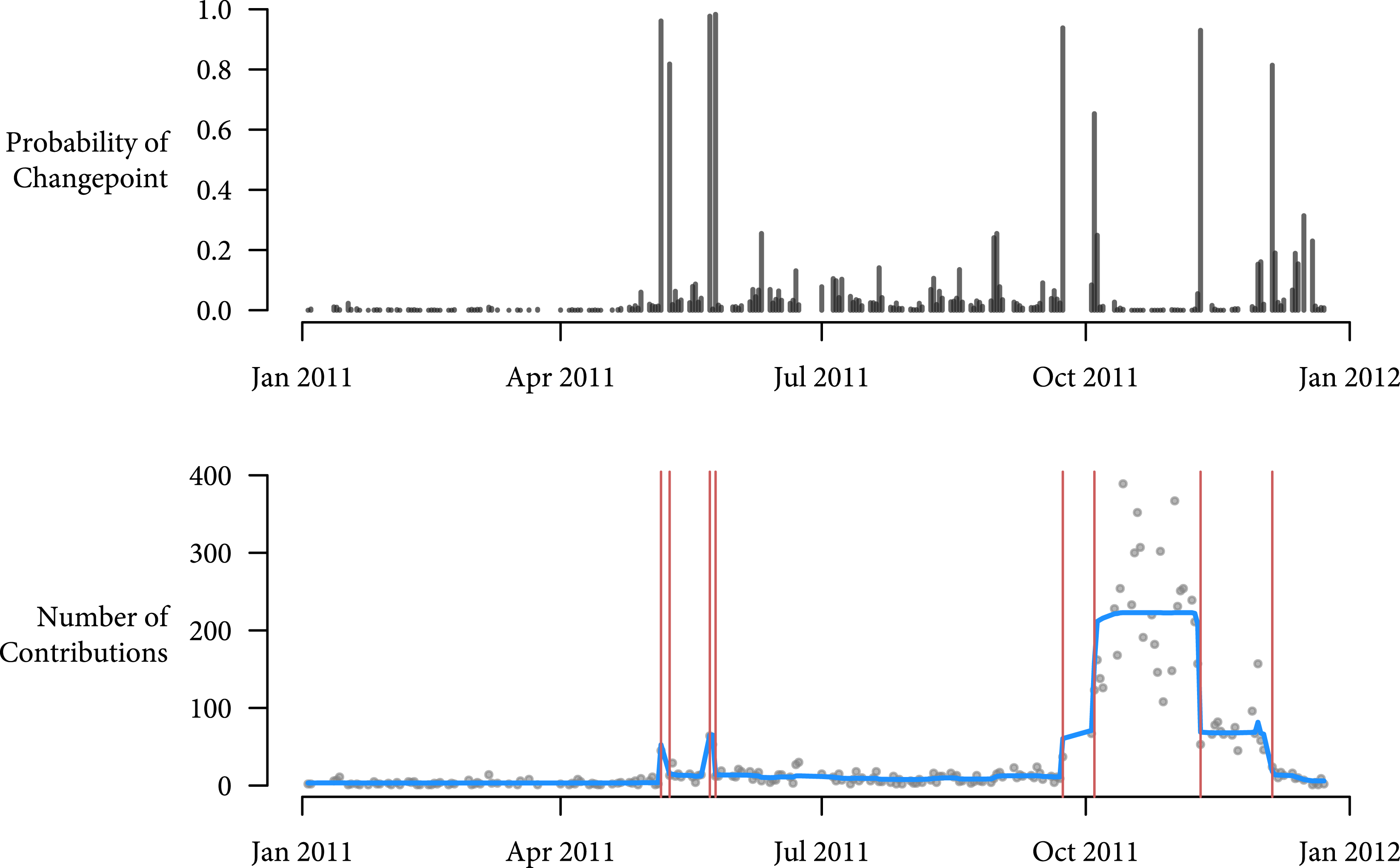
Figure 1. Contributions and changepoints for Herman Cain in the 2012 Republican Primary.
Figure 1 presents the posterior probability of a changepoint in the top panel.Footnote
4
In the bottom panel, I plot the raw number of contributions along with the posterior mean of $\unicode[STIX]{x1D706}_{t}$
, the mean of the negative binomial distribution for each observation in red. The vertical red lines correspond to dates that have greater than 0.5 posterior probability of being a changepoint. Table 1 lists each of these estimated changepoints and its corresponding event in the campaign. The model correctly identifies major shifts in the distribution of contributions to Herman Cain that correspond to actual prominent events in his campaign. The model correctly identifies his rise after winning a key straw poll on September 24th, 2011, (Sutton and Holland Reference Sutton and Holland2011) and his fall after sexual misconduct allegations were made public on November 7th (Henderson Reference Henderson2011; Palmer et al.
Reference Palmer, Martin, Haberman and Vogel2011). Note that the model makes no restrictions on the number of changepoints in the data. This is crucial in this example because specifying the number of changepoints a priori would be difficult, even if one were to visually inspect the time series.
$\unicode[STIX]{x1D706}_{t}$
, the mean of the negative binomial distribution for each observation in red. The vertical red lines correspond to dates that have greater than 0.5 posterior probability of being a changepoint. Table 1 lists each of these estimated changepoints and its corresponding event in the campaign. The model correctly identifies major shifts in the distribution of contributions to Herman Cain that correspond to actual prominent events in his campaign. The model correctly identifies his rise after winning a key straw poll on September 24th, 2011, (Sutton and Holland Reference Sutton and Holland2011) and his fall after sexual misconduct allegations were made public on November 7th (Henderson Reference Henderson2011; Palmer et al.
Reference Palmer, Martin, Haberman and Vogel2011). Note that the model makes no restrictions on the number of changepoints in the data. This is crucial in this example because specifying the number of changepoints a priori would be difficult, even if one were to visually inspect the time series.
Table 1. Estimated Herman Cain changepoints and their substantive explanations. $\Pr (\text{Change})$
gives the posterior probability of changepoint on the given dates.
$\Pr (\text{Change})$
gives the posterior probability of changepoint on the given dates.

3.2 Terrorism around the world
Terrorism remains a persistent and malevolent threat in many countries around the world, and how terrorism relates the political world has generated considerable scholarly interest (see Young and Findley Reference Young and Findley2011, for a review of this literature). Many of these studies leverage time-series or time-series cross-sectional data on terrorist attacks or the number of injuries due to terrorist attacks. These time series tend to be highly overdispersed, however, since a single attack might induce many clustered injuries or an underlying conflict may lead to “bundles” of attacks in a given country.
To investigate changes in the distribution of terrorist attacks over time, I analyze data from the Global Terrorism Database (Terrorism 2016), which tracks both transnational and domestic terror attacks from 1970 until 2015 (with 1993 missing). I aggregate the number of deaths and number wounded in terrorist attacks to the monthly level to produce a time series of terrorism-related injuries over 552 months. With this long span of data and quite a few outlier months, allowing the data to choose the number of regimes is vital. Identifying changepoints and common regimes can elucidate some of the root causes of terrorism and point researchers to time periods and events worthy of further study.

Figure 2. Top panel is a heatmap of the posterior probability of two months being in the same regime, with more pink colors denoting two months having higher posterior probabilities of belonging to the same regime. Bottom panel is the time series of the raw data. Red vertical lines highlight months with greater than 0.5 probability of being a changepoint.
Figure 2 presents the results of the model for the terrorism data. The top panel of this figure shows the posterior probability of two time periods being in the same regime, and the bottom panel shows the counts over time. Red vertical lines represent dates with a greater than 0.5 posterior probability of being a changepoint. The clearest message from these results is the relative stability of terrorism in the Cold War era and the relative instability after the USSR collapses in 1991. In the latter era, a few changepoints highlight single months that had an unusually high number of injuries, such as the 9/11 attacks, the August 1998 U.S. embassy bombings, and a combination of the Tokyo sarin gas subway attacks and the Oklahoma City bombing in March and April of 1995, respectively.
There are several changepoints since 9/11, each marking a significant increase in terrorist activity. After June 2006, for instance, the terrorism-induced injury rate in Iraq, Pakistan, India, and Afghanistan increased markedly. Another increase in terrorist attack occurs at the start of 2012, with significantly increased terrorist activity from jihadist groups such as the Taliban (in Afghanistan and Pakistan), Al-Shabaab (East Africa), Al-Qaida in Iraq, and Boko Haram (West Africa). A final regime starts in May of 2013 and continues through the end of the data (late 2015), with increases in activity by all of these groups and the beginning of attacks from the Islamic State of Iraq and the Levant (ISIL). The changepoint that precipitates this final regime coincides with two events. First, there is an escalation of the conflict between Nigeria and Boko Haram. Second, Sunni–Shia violence erupted in May 2013 in reaction to the Iraqi Army raiding an anti-government protest camp in the city Hawija in northern Iraq amid tension surrounding the April parliamentary elections.
Even without guidance on the number or location of structural breaks, the model is able to find politically relevant dates where the distribution of terrorist activity sharply changed. Previous studies have generally found different changepoints than the ones found here, but these studies generally focused on incident counts by type.Footnote 5 Note that extending this model to include region parameters or covariates as is common in the literature would be straightforward. In this augmented model, changepoints would detect when the overall level of terrorism or the distribution of terrorism across region changes or if the effect of various covariates changes.
4 Conclusion
This paper applies a novel statistical model that estimates the number and timing of changepoints in overdispersed count data. This model, which relies on Bayesian nonparametrics, gives researchers the ability to cluster political time series into distinct regimes and detect significant shifts in the distribution of the counts. The model uses recent developments in Dirichlet process priors to estimate the number of changepoints rather than specifying the number a priori. This is important in many applications where the number of changepoints is unknown or is the target of inference itself. While the model here has been tailored to overdispersed count data, modifying the base (within-regime) model to allow for continuous, binary, and ordered categorical outcome variables is possible.
Supplementary materials
For supplementary materials accompanying this paper, please visithttps://doi.org/10.1017/pan.2017.42.


