2 Setup

We consider a randomized or natural experiment with subjects indexed by $i=1,\dots ,N$ , for which we also have measured P pre-treatment covariates collected in the vector $\mathbf {X}_i = (X_{i1}, X_{i2}, \dots , X_{iP})$ . For each subject, we always observe values of the covariates,Footnote ² the treatment status $D_i \in \{0,1\}$ , and the response indicator $S_i \in \{0,1\}$ . The realized outcome $Y_i$ is observed only when $S_i = 1$ . For $D_i = 1$ and $D_i=0$ , respectively, potential outcomes are given by $(Y_i(1), Y_i(0))$ and potential response indicators are given by $(S_i(1), S_i(0))$ . The realized response indicator is $S_i = D_iS_i(1) + (1-D_i)S_i(0)$ , and the realized outcome is $Y_i = D_iY_i(1) + (1-D_i)Y_i(0)$ when $S_i = 1$ and missing when $S_i = 0$ . Define $U_i$ to be unobserved factors that affect both $(S_i(1),S_i(0))$ and $(Y_i(1),Y_i(0))$ .

We make the following assumption on treatment assignment:

Assumption 1. Strong ignorability:

The first part states that the treatment is conditionally independent to both the potential outcomes and the potential responses. The second part requires that the propensity score, $p(\mathbf {X}_i) = P(D_i = 1 | \mathbf {X}_i)$ , is strictly bounded between 0 and 1.Footnote ³ The assumption holds in experiments when treatment is randomly or conditionally randomly assigned. In observational studies, the assumption implies that the covariate vector $\mathbf {X}_i$ includes all confounders.

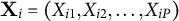
The directed acyclic graph (DAG) in Figure 1 shows relationships that our setting admits. For the Santoro and Broockman (Reference Santoro and Broockman2022) study, $U_i$ could represent the degree of political interest. Our approach also admits the possibility that $Y_i$ directly affects missingness. Only using observations with $S_i = 1$ amounts to conditioning on $S_i$ , which is a “collider” between the treatment $D_i$ and then either the unobserved $U_i$ or the outcome $Y_i$ (Elwert and Winship Reference Elwert and Winship2014; Montgomery et al. Reference Montgomery, Nyhan and Torres2018). For example, suppose that for some units, $D_i$ and $U_i$ negatively affect response. For these units, high values of $D_i$ (i.e., being treated) would tend to require low values of $U_i$ for $S_i = 1$ to hold. The lower $U_i$ values would affect the distribution of $Y_i$ values. Correlations induced by conditioning on $S_i = 1$ confound our ability to estimate the causal effect of $D_i$ on $Y_i$ . Such induced correlations result in bias.

Figure 1

Endogenous missingness.

Note: The above figure shows a directed acyclic graph (DAG) representing an endogenous missingness mechanism. White nodes represent observable variables and black nodes represent unobservable ones. An arrow from one node to the other (a “path”) marks the causal relationship from the former to the latter. The heavier arrows indicate the relationships that generate the bias from conditioning on $S_i$ .

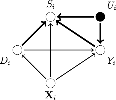
To further understand the source of the bias, we classify subjects into four different types based on their responses to the treatment: always-responders ( $S_i(0) = S_i(1) = 1$ ), never-responders ( ${S_i(0) = S_i(1) = 0}$ ), treatment-only responders ( $S_i(0) = 0, S_i(1) = 1$ ), and control-only responders ( ${S_i(0) = 1, S_i(1) = 0}$ ). These subgroups are examples of what Frangakis and Rubin (Reference Frangakis and Rubin2002) call “principal strata,” similar to those in the setting with instrumental variables (Angrist, Imbens, and Rubin Reference Angrist, Imbens and Rubin1996). These strata are determined by the attributes of the units, such as $\mathbf {X}_{i}$ and $U_i$ , but not affected by treatment assignment. From Table 1 (Panel 1), we see that among units with observed outcomes ( $S_i=1$ ), the control group may consist of both control-only responders (CR) and always-responders (AR), while the treatment group is a mixture of treatment-only responders (TR) and always-responders (AR). Therefore, the group-mean difference in the observed outcome does not capture an average of treatment effects for a fixed sub-population.

Table 1

Principal strata.

Note: AR, NR, TR, and CR in the table stand for always-responders, never-responders, treatment-only responders, and control-only responders, respectively.

From the decomposition in Table 1 (Panel 1), we cannot identify the share of units falling into each principal stratum from data. Following Lee (Reference Lee2009), we consider the following assumption on the selection process:

Assumption 2. Monotonic selection:

$$ \begin{align*} S_i(1) \ge S_i(0) \end{align*} $$

for any i.

The assumption requires that under treatment, a unit is at least as likely to respond as under control, thus it excludes the existence of control-only responders. This is shown in Table 1 (Panel 2). The assumption is similar to the “no defiers” assumption for instrumental variables. It should be motivated by arguments about the choice behavior of agents determining response (Slough Reference Slough2023). We could alternatively assume the opposite: $S_i(1) \le S_i(0)$ for any i. Then, we have control-only responders but not treatment-only responders. Either form of monotonicity allows one to form trimming bounds. In the Santoro and Broockman (Reference Santoro and Broockman2022) example, subjects who would engage when uninformed of their partners’ partisanship would be assumed to engage when informed.Footnote ⁴ Parametric and semi-parametric selection models implicitly impose a monotonicity assumption as part of the first-stage regression specification (Vytlacil Reference Vytlacil2002); the manner in which we state monotonicity here is a nonparametric generalization.

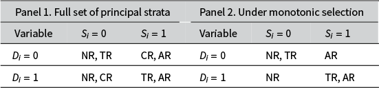
Table 2 reports how examples from different fields of political science (American politics, comparative politics, public administration, international relations, and political economy) fit into our setup.

Table 2

Empirical examples

Note: This table summarizes how examples from different fields of political science fit into the setup developed here.

3 Trimming Bounds

Lee (Reference Lee2009) shows that we can use “trimming” to bound the average treatment effect for always-responders, , under Assumptions 1 and 2. The focus on always-responders has substantive motivation. It is the subset of the population that would not withdraw (or be withdrawn) from the intervention under prevailing circumstances. It is also the subset of the population for which intensive margin effects are defined (as in Lee’s original application). Table 2 lists examples.

To lighten the notation in the discussion that follows, suppose that we have unconditionally random assignment. For the more general analysis under strong ignorability (Assumption 1), one would simply switch the expectations to include iterated expectations that condition on and then marginalize over $\mathbf {X}_i$ . Given this notational convenience, the average treatment effect for always-responders can be expressed as

$$ \begin{align*} \tau(1,1) & := E[Y_{i}(1) | S_{i}(1) = S_{i}(0) = 1] - E[Y_{i}(0) | S_{i}(1) = S_{i}(0) = 1] \\ & = E[Y_{i} | D_i = 1, S_{i}(1) = S_{i}(0) = 1] - E[Y_{i} | D_i = 0, S_i = 1]. \end{align*} $$

The result indicates that under random assignment and monotonic selection, the mean of observed outcomes in the control group identifies the average untreated outcome for the always-responders. Those who respond in the treatment group can belong to either always-responders or treatment-only responders, and so the observed mean does not identify the average treated outcome for the always-responders.

Recall that Assumption 1 implies that the shares of units in each principal stratum are balanced (in expectation) across treatment and control. Under Assumption 2, the rate at which outcomes are observed in the control group, $\text {Pr}[S_i = 1 \mid D_i = 0]$ , identifies the share of units in the overall sample that are always-responders. The rate at which outcomes are observed in the treatment group, $\text {Pr}[S_i = 1 \mid D_i = 1]$ , identifies the share of units in the overall sample that are either treatment-only responders or always-responders. If we let q denote the share of treated units with observed outcomes that are always-responders, then we have

$$ \begin{align*}q = \frac{\text{Pr}[S_i = 1 \mid D_i = 0]}{\text{Pr}[S_i = 1 \mid D_i = 1]}. \end{align*} $$

The mean of observed outcomes in the treatment group can be written as a mixture of the always-responders mean (with weight q) and the treatment-only responders mean (with weight $1-q$ ):

$$ \begin{align*} E[Y_{i} | D_i = 1, S_i = 1] &= q E[Y_{i} | D_i = 1, S_{i}(1) = S_{i}(0) = 1] \\ &\quad + (1-q)E[Y_{i} | D_i = 1, S_{i}(1) = 1, S_{i}(0) = 0]. \end{align*} $$

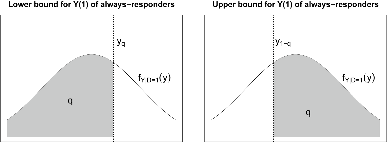
The quantity $E[Y_{i} | D_i = 1, S_{i}(1) = S_{i}(0) = 1]$ is not identified under random assignment and monotonicity. But we can construct sharp upper and lower bounds that surround it by trimming the lower and upper tails of the observed treated outcome distribution by the share of treatment-only responders, thus retaining the portion with mass q (Lee Reference Lee2009, Proposition 1a). As shown in Figure 2, in the worst case, always-responders take the bottom (left-most) q share of the treated outcome’s distribution. Hence, the average treated outcome of always-responders is bounded from below by $Y(1)$ ’s expectation over the shaded area in the left plot. Similarly, the average treated outcome for always-responders is bounded from above by $Y(1)$ ’s expectation over the shaded area in the right plot. Mathematically, we have

$$\begin{align*}\begin{aligned} E[Y_{i} | D_i = 1, S_i = 1, Y_i \leq y_{q}] & \leq E[Y_{i} | D_i = 1, S_{i}(1) = S_{i}(0) = 1] \\ & \leq E[Y_{i} | D_i = 1, S_i = 1, Y_i \geq y_{1-q}], \end{aligned} \end{align*}$$

where $y_{q}$ is the qth-quantile of the observed outcome’s conditional distribution in the treatment group that satisfies the condition $\int _{-\infty }^{y_{q}} dF_{Y|D=1, S=1}(y) = q$ . Here, $F_{Y|D=1, S=1}(\cdot )$ is the distribution function for observed treatment group outcomes. The quantile $y_{1-q}$ is similarly defined. We denote $E[Y_{i} | D_i = 1, S_i = 1, Y_i \leq y_{q}] - E[Y_{i} | D_i = 0, S_i = 1]$ as $\tau ^L_{TB}(1, 1)$ and $E[Y_{i} | D_i = 1, S_i = 1, Y_i \geq y_{q}] - E[Y_{i} | D_i = 0, S_i = 1]$ as $\tau ^U_{TB}(1, 1)$ , where TB is short for trimming bounds. Clearly,

$$ \begin{align*}\tau^L_{TB}(1, 1) \leq \tau(1, 1) \leq \tau^U_{TB}(1, 1). \end{align*} $$

The interval $[\tau ^L_{TB}(1, 1), \tau ^U_{TB}(1, 1)]$ is the identified set for the always-responder treatment effect.

Figure 2

Basic trimming bounds in Lee (Reference Lee2009).

4 Covariate-Tightened Trimming Bounds

Basic trimming bounds that do not incorporate covariate information can be very wide. Lee (Reference Lee2009, Proposition 1b) suggests that when covariates are discrete, researchers can estimate the bounds across blocks formed by them for more precise inference. We extend this approach to cases where the covariates are continuous or large in number. For $\mathbf {X}_i = \mathbf {x}$ , consider the always-responders’ conditional average treatment effect, . We can derive the following bounds using the same logic as above:

$$\begin{align*}\begin{aligned} E[Y_{i} | D_i = 1, S_i = 1, Y_i \leq y_{q(\mathbf{x})}(\mathbf{x}), \mathbf{X}_i = \mathbf{x}] & \leq E[Y_{i} | D_i = 1, S_{i}(1) = S_{i}(0) = 1, \mathbf{X}_i = \mathbf{x}] \\ & \leq E[Y_{i} | D_i = 1, S_i = 1, Y_i \geq y_{1-q(\mathbf{x})}(\mathbf{x}), \mathbf{X}_i = \mathbf{x}], \end{aligned} \end{align*}$$

where $q(\mathbf {x})$ is the conditional proportion of always-responders among units with observed outcomes in the treatment group; $y_{q(\mathbf {x})}(\mathbf {x})$ and $y_{1-q(\mathbf {x})}(\mathbf {x})$ are the conditional $q(\mathbf {x})$ -quantile and $(1-q(\mathbf {x}))$ -quantile of the conditional treated outcome distribution.

We denote the conditional control mean for always-responders, $E[Y_{i} | D_i = 0, S_i = 1, \mathbf {X}_i = \mathbf {x}]$ , as $\theta _{0}(\mathbf {x})$ , $E[Y_{i} | D_i = 1, S_i = 1, \mathbf {X}_i = \mathbf {x}, Y_i \leq y_{q(\mathbf {x})}(\mathbf {x})]$ as $\theta _{1}^{L}(\mathbf {x})$ , and $E[Y_{i} | D_i = 1, S_i = 1, \mathbf {X}_i = \mathbf {x}, Y_i \geq y_{1-q(\mathbf {x})}(\mathbf {x})]$ as $\theta _{1}^{U}(\mathbf {x})$ , respectively. Then,

where CTB is short for covariate-tightened trimming bounds. The conditional bounds allow us to see how the bounds vary across different values of the covariates. In practice, we can either estimate the conditional bounds for all the observations or over evaluation points spanning the covariate distribution of the sample. For instance, we can generate the evaluation points by going through the quantiles of one covariate while fixing the values of the other covariates at their sample mode or average.

We can further integrate ( $\tau _{CTB, \mathbf {x}}^L(1,1)$ , $\tau _{CTB, \mathbf {x}}^U(1,1)$ ) over the distribution of $\mathbf {X}_i$ among always-responders to recover the unconditional covariate-tightened bounds on $\tau (1, 1)$ . Define

where

$$ \begin{align*} q_0(\mathbf{x}) := \Pr[S_i(1) = S_i(0) = 1 \mid \mathbf{X}_i = \mathbf{x}] = \Pr[S_i = 1 \mid D_i = 0, \mathbf{X}_i = \mathbf{x}] \end{align*} $$

is the expected conditional proportion of always-takers in the overall sample and $F(\mathbf {x})$ is the distribution of the covariates. The expression indicates that $q_0(\mathbf {x})$ can be identified from the control group. In expectation, covariate-tightened trimming bounds will not be wider than the basic trimming bounds:Footnote ⁵

$$ \begin{align*}\tau^L_{TB}(1, 1) \leq \tau^L_{CTB}(1, 1) \leq \tau(1, 1) \leq \tau^U_{CTB}(1, 1) \leq \tau^U_{TB}(1, 1). \end{align*} $$

The improvement depends on how well the covariates predict the outcome or response rate (Semenova Reference Semenova2025). These bounds are also sharp—we cannot further reduce the identified set’s width without additional information.

We can also relax Assumption 2 and allow the direction of monotonicity to change across the values of covariates, as suggested by Semenova (Reference Semenova2025). We replace Assumption 2 with the following:

Under Assumption 3, the covariates space X can be divided into two parts, $\mathcal {X}^{+}$ and $\mathcal {X}^{-}$ , that satisfy

$$ \begin{align*}\begin{cases} S_i(1) \le S_i(0), & \mathbf{X}_i \in \mathcal{X}^{-} \\[4pt]S_i(1) \ge S_i(0), & \mathbf{X}_i \in \mathcal{X}^+ \end{cases} \text{where } \mathcal{X}^{+} \cup \mathcal{X}^{-} = \mathcal{X}. \end{align*} $$

To identify $\mathcal {X}^+$ and $\mathcal {X}^-$ , we first estimate the conditional trimming probability, $q(\mathbf {x})$ , and approximate $\mathcal {X}^+$ and $\mathcal {X}^-$ with and , respectively. Semenova (Reference Semenova2025) shows that the classification is accurate in large samples under regularity conditions. If the sample is substantially divided between sets $\hat {\mathcal {X}}^{-}$ and $\hat {\mathcal {X}}^{+}$ , conditional monotonicity would be more plausible than unconditional monotonicity. Conditional on each part, we can estimate either the conditional or the aggregated bounds. To acquire the aggregated bounds for the whole sample, we take a weighted average the estimates from $\mathcal {X}^{+}$ and $\mathcal {X}^{-}$ .

Conditionally monotonic selection (Assumption 3) is weaker than its unconditional counterpart (Assumption 2). It also seems uncontroversial that there could be both control-only and treatment-only responders in a sample, even if Lee’s original analysis ruled this out. In the Santoro and Broockman (Reference Santoro and Broockman2022) experiment, treatment may induce missingness for those who find it aversive to speak to an outpartisan, while it may reduce missingness for those who find it boring to talk to a “random person.” That said, the interpretation of conditionally monotonic selection can be subtle. The assumption holds when, at any point in the covariate space, units for which outcomes are observed are either a mixture of always-responders and control-only responders or a mixture of always-responders and treatment-only responders. If there are values of $\mathbf {X}_i$ in which control-only responders and treatment-only responders are both present, then the assumption is violated. The share of always-responders can vary arbitrarily over covariate values, and so it may not be obvious exactly where in the covariate space transitions occur from regions containing control-only responders versus treatment-only responders. In our algorithm, we use units’ covariates to classify them as being in either the (1) always-responders + control-only responders class or (2) always-responders + treatment-only responder class. Our algorithm would be inconsistent if, asymptotically, the covariates are inadequate to perform such a classification. There may be ways to further adjust the bounds to account for such residual classification error. We consider this issue to be beyond the scope of the current paper but one that we think is interesting for further research. We do note that our implementation and accompanying package contains an option to set a tolerance parameter for how sensitive is the classification.

We can also consider the relationship between conditionally monotonic selection and the conditional independence (“missing at random,” MAR) assumption that motivates approaches such as imputation, regression adjustment, or inverse propensity score weighting. One can construct scenarios where conditionally monotonic selection is satisfied while MAR is violated, and vice versa. Importantly, however, the bounding approach allows unmeasured variables to affect both response and the outcome, as demonstrated by our DAG in Figure 1, which we understand to be a first-order threat to identification. In cases where an unobserved variable affects response patterns in a conditional-monotonicity fashion, a MAR approach is biased but we would still be able to recover valid trimming bounds, as we show in Section D.1 of the Supplementary Material. In contrast, when an unobservable variable affects the direction of missingness, even after conditioning on covariates, but is strictly independent of outcomes, then MAR would hold but Assumption 3 would fail. The latter scenario strikes us as more unusual than the former, although we appreciate that this does not exhaust all possibilities.

In Section C of the Supplementary Material, we demonstrate extensions to unit-level missing data, binary outcomes, and estimated propensity scores for generalizing to observational studies under strong ignorability.

5 Estimation

Estimating the covariate-tightened trimming bounds proceeds in two steps. First, we estimate the “nuisance parameters”, $(q_0(\mathbf {x}), q_1(\mathbf {x}))$ and $(y_{q(\mathbf {x})}(\mathbf {x}), y_{1-q(\mathbf {x})}(\mathbf {x}))$ . Second, we use the nuisance parameter estimates to estimate the “target parameters,” that is, the conditional bounds or the aggregated bounds. To estimate parameters evaluated at point $\mathbf {x}$ , we use the generalized random forest (grf) method. The grf method approximates quantities at $\mathbf {x}$ using a weighted average of neighboring observations. To determine the weights, grf generates many regression trees from randomly selected sub-samples, and the weight given to observation i for a prediction at $\mathbf {x}$ equals the share of trees in which i falls in the same leaf as the value $\mathbf {x}$ . Compared to standard kernel weighting, the grf weights are adaptive to the sample distribution and better manage the bias-variance tradeoff. Following Chernozhukov et al. (Reference Chernozhukov2018), our algorithm also incorporates Neyman orthogonalization and cross-fitting to avoid biases from using the same data to fit nuisance and target parameters, while also maintaining efficiency. The bounds estimators are shown to be asymptotically normal, therefore confidence interval construction is straightforward. Practitioners can also directly construct confidence intervals for $\tau (1,1)$ , the ATE for always-responders, using methods developed by Imbens and Manski (Reference Imbens and Manski2004) and Stoye (Reference Stoye2009). Figure 1 summarizes the algorithm. Technical details and statistical properties are given in the Supplementary Material.

6 Simulation

We conduct a Monte Carlo experiment to study the method’s performance. We set $N=1,000$ and the number of covariates $P=10$ . Each of the covariates, $X_p$ , is drawn from the uniform distribution on $[0, 1]$ . The unobservable factor, U, is uniform on $[-1.4, 1.4]$ . We only allow $X_1$ and U to affect both the potential responses ( $S_i(0)$ , $S_i(1)$ ) and the potential outcomes ( $Y_i(0)$ , $Y_i(1)$ ), while the other nine covariates are pure noise. The setup resembles the reality in which we possess measures of multiple covariates but do not know ex-ante which one(s) should be controlled. Our exact data-generating process is as follows:

$$ \begin{align*}\begin{aligned} & Y_i(0) = 1.5 - 2*U_{i}^2 + 4*X_{1i} + \varepsilon_{i}, \\ & Y_i(1) = Y_i(0) + 2.5 + 1.8*U_{i} + 3*\sin(-0.7 + 2*X_{1i}), \\ & S_i = \mathbf{1}\{1 - 0.2*X_{1i} - 1.6*|U_{i}| + 0.4*D_i + 0.1*D_i*X_{1i} + 2.2*D_i*|U_{i}| + \nu_i> 0 \}, \\ & D_i \sim Bernoulli(0.5), \varepsilon_{i} \sim \mathcal{N}(0, 1), \nu_{i} \sim \mathcal{N}(0, 1). \end{aligned} \end{align*} $$

Individualistic treatment effects are nonlinear and non-monotonic in the covariates. Both the selection indicator $S_i$ and outcome $Y_i$ are affected by $D_i$ and $U_i$ , making the sample selection process endogenous. The construction of $S_i$ guarantees that $S_i(1) \geq S_i(0)$ per Assumption 2.

We first estimate the conditional bounds, ( $\tau ^L_{CTB, \mathbf {x}}(1,1)$ , $\tau ^U_{CTB, \mathbf {x}}(1,1)$ ), across 19 points where $X_2$ to $X_{10}$ are fixed at their sample averages, with $X_1$ values set at 5ppt. increments. The results are shown in the right plot of Figure 3. Each gray point is an individual-level treatment effect for an observation from one of the Monte Carlo samples. The black line traces out the true CATE for the always-responders; this quantity would be unobservable in a real application and constitutes what the conditional bounds should cover. Upper bounds estimates are depicted as red dots and lower bounds estimates as blue dots. The dotted lines surrounding them are the estimated 95% confidence intervals. The red and blue curves are the true bounds on the always-responders CATEs, based on the simulation parameters. The estimates are very accurate in the middle part of $X_1$ ’s support but slightly biased at the boundary points.

Figure 3

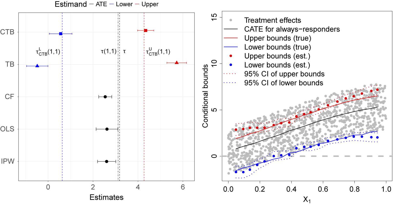
Covariate-tightened trimming bounds in simulated data.

Note: The plot on the left shows the averages of the covariate-tightened trimming bound estimates (CTB, in squares), basic trimming bounds (TB, in triangles), ATE estimate using causal forest on the non-missing sample (CF, in circles), ATE estimate using OLS on the non-missing sample (OLS, in circles), and ATE estimate using OLS re-weighted by the inverse probability of attrition (IPW, in circles). Lower bound estimates are in blue and upper bound estimates are in red. The segments represent 95% confidence intervals. The red and blue dotted lines mark the CTBs. The black dotted line represents the true ATE and the black dash dotted line represents the true ATE for the always-responders. The plot on the right shows the estimates of the conditional covariate-tightened trimming bounds across 19 evaluation points on $X_1$ , holding $X_2$ to $X_{10}$ to their sample averages.

In the left plot of Figure 3, the top row presents the averages of our CTB estimates with 95% confidence intervals across 1,000 treatment assignments. It is clear that our estimates lead to a narrower identified set of $\tau (1,1)$ , the ATE for always-responders, than unadjusted bounds (“TB”). The estimates are also centered around the true CTB and the standard errors of our estimates are not larger than the unadjusted bound estimates. Estimates of the ATE using causal forest or OLS on the non-missing sample and OLS with inverse probability of attrition weighting (IPW) are biased given endogeneity to the unobserved U.Footnote ⁶

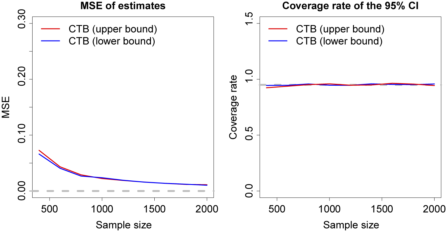
We examine the asymptotic properties of our estimators by varying the sample size from 400 to 2,000. In Figure 4 shows how mean squared error (MSE) and the confidence interval coverage rates perform as N goes from 400 to 2,000, still over 1,000 Monte Carlo draws. MSE declines toward zero as N grows, and our method provides the correct (95%) coverage across the sample sizes. In the Supplementary Material, we present evidence that the performance of the method remains stable when the number of features in the data increases and is superior to alternative methods proposed by Olma (Reference Olma2020) and Semenova (Reference Semenova2025).

Figure 4

Asymptotic performance of the method.

Note: The left panel shows how the MSE of the lower bound estimate (in blue) and upper bound estimate (in red) varies with sample sizes. The right panel presents the variation of the coverage rate across sample sizes. The gray line marks the nominal level of coverage, 95%.

7 Application

We apply our methods to study the robustness of the findings from Santoro and Broockman (Reference Santoro and Broockman2022) to potentially endogenous attrition. Our Supplementary Material reanalyzes the Job Corps study, which was the original application in Lee (Reference Lee2009), as well as a study by Kalla and Broockman (Reference Kalla and Broockman2022) to demonstrate a binary outcome and a study by Blattman and Annan (Reference Blattman and Annan2010) to demonstrate an observational study.

We focus on Santoro and Broockman (Reference Santoro and Broockman2022, Study 1), which invited subjects to have a video chat on an online platform with a partner from a different party. The theme of the conversation is what their perfect day would be like. The study started with 986 subjects who satisfied the screening criteria. The subjects were then randomly assigned into either the treatment group ( $D_i = 1$ ), in which they were informed that the partner would be an outpartisan, or the control group ( $D_i = 0$ ), in which they received no extra information. Among subjects that were assigned to a treatment condition, 45.2% of the treated subjects and 39.5% of the control subjects completed the conversation and post-treatment survey. The authors examined the treatment effect on attitudes toward the other parties and found significant effects in the short run.

The authors indicate that the treatment effect on the response rates had a p-value of 0.055, and their omnibus test for covariate balance with respect to education, race/ethnicity, gender, age, and party identification had a p-value of 0.28. Nonetheless, the difference in response rates is not trivial, and other confounding factors may be imbalanced beyond those tested. We can use our covariate-tightened trimming bounds to assess the robustness of their findings. Our inference targets the “always responders” that would complete the conversation and survey regardless of being informed about their partner’s partisanship. We focus on the “warmth toward outpartisan voters” outcome (measured by a rescaled thermometer) and rely on the same covariates the authors selected for their analysis, including the age, gender, race, education level, and party identification of the subjects, as well as their pre-treatment outcome.

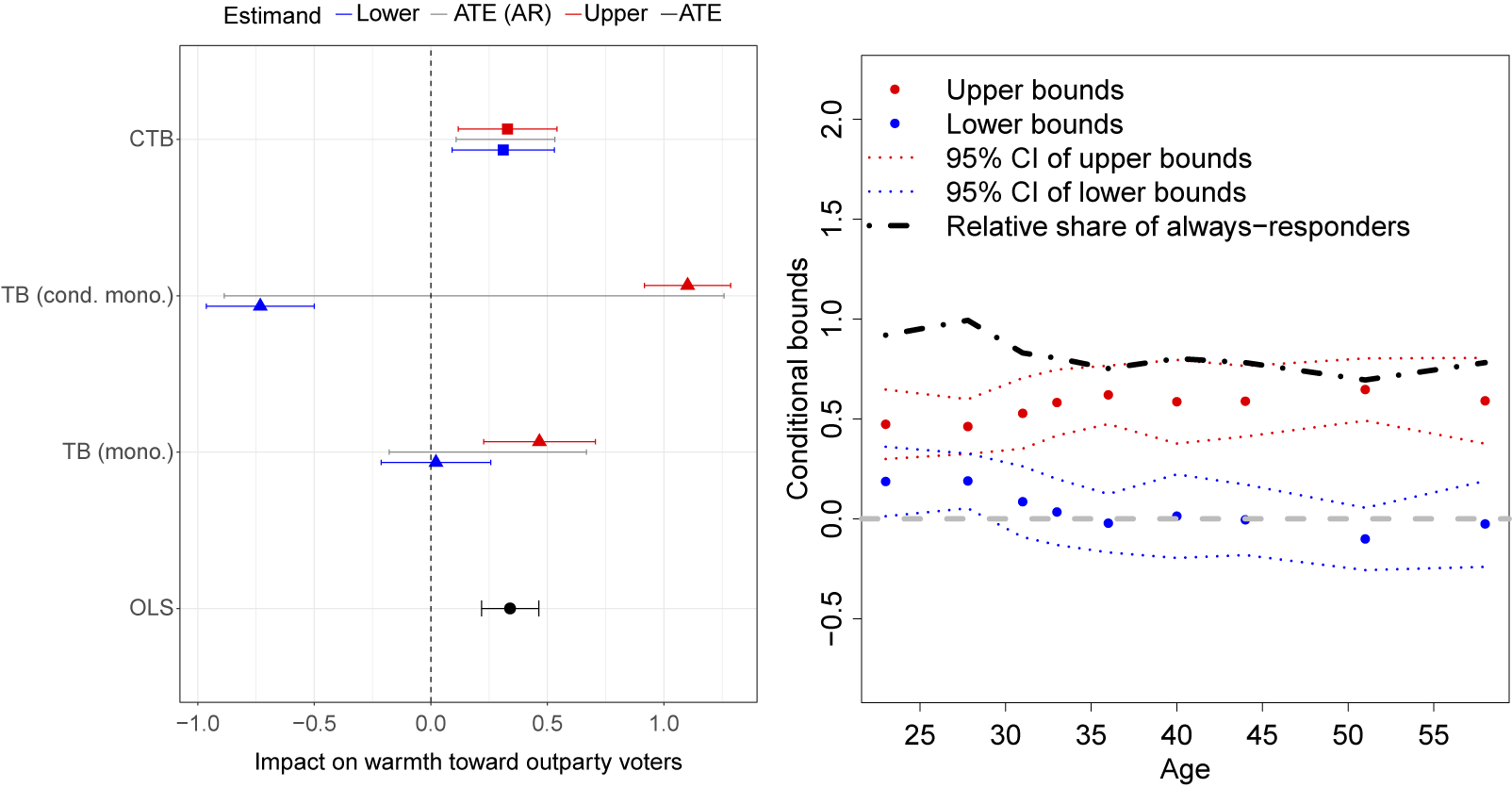
Figure 5 shows the results. At the bottom is the OLS estimate replicating the main result in the paper. Above that (TB mono.) are the basic trimming bounds, assuming monotonic selection. In this case, however, unconditional monotonicity is questionable. While the overall pattern was such that missingness was lower in the treatment group, some types of people (e.g., those with high affective polarization) may actually choose to drop out when informed about their partner’s partisan status. When we perform the test proposed in the discussion of conditional monotonicity above, the results suggest that unconditional monotonicity is violated (see the Supplementary Material for details). We thus construct two sets of units ( $\mathcal {X}^{+}$ and $\mathcal {X}^{-}$ ) for which treatment is positively and negatively associated with response. Basic trimming bounds (without covariate adjustment) for the first group would be based on bounding the treated mean, and bounds for the second group are based on bounding the control mean. We can form the basic trimming bounds for the overall sample by constructing the appropriately weighted average of these bounds and the observed treated and control means. The result is shown as “TB (cond. mono.).” We see that relaxing the monotonic selection assumption has strong consequences for our inference. However, when we adjust for covariates using our proposed method (“CTB”), we get tighter results that also allow for conditionally monotonic selection. Both the lower bound ( $0.272$ ) and the upper bound ( $0.355$ ) are significantly larger than zero, suggesting that the ATE for the always-responders is indeed positive.

Figure 5

Covariate-tightened trimming bounds in Santoro and Broockman (Reference Santoro and Broockman2022).

Note: In both plots, the outcome variable is warmth toward outpartisan voters. The plot on the left shows the estimated covariate-tightened trimming bounds (CTB, in squares), basic trimming bounds under monotonicity (TB (mono.), in triangles) and under conditional monotonicity (TB (cond. mono.), in triangles), and the ATE estimate using OLS on the non-missing sample (OLS, in circles). Lower bound estimates are in blue and upper bound estimates are in red. Segments represent the 95% confidence intervals for the estimates. Black segments between the red and blue ones represent the 95% confidence intervals for the ATE for always-responders, using the Imbens–Manski approach. The plot on the right shows the estimates of the conditional covariate-tightened trimming bounds across nine evaluation points of age with other demographic attributes are fixed to sample mean or mode.

We can examine how the bounds vary over the age of the subjects. We create nine “representative subjects” whose demographic attributes are fixed at the sample mean or mode while their age varies across its deciles. The estimates of the conditional bounds are shown in the right plot of Figure 5. The red and blue dots represent the upper and the lower bounds, respectively, while the dotted lines around them are the 95% confidence intervals. The dash-dotted curve depicts the conditional trimming probability. The response rate (which determines the share of always-responders) is much higher among subjects who are younger than 30. The conditional lower bounds are also significantly larger than zero for this sub-group, while the identified set crosses zero for other subjects. We show results for pre-treatment warmth and ideology in the Supplementary Material.