


1 Introduction
When two variables are simultaneously generated, it becomes challenging and promising to study the relationship between them. For instance, if unobserved confounders affect them, regressing one variable on the other leads to endogeneity bias. Scholars may have reasonable substantive knowledge or theory about the marginal distributions of the two variables but no idea about the conditional distribution of one variable given the other. One approach is to directly analyze the joint distribution. When one variable includes some of the same information as the other, analyzing them together will lead to less biased and more efficient estimation, as well as better prediction without assuming selection on observables. Classic methods include the seemingly unrelated regression and Heckman’s sample selection models, although they assume only a bivariate normal distribution for the variables.Footnote 1 Instead, as I elaborate on below, copula functions are flexible and helpful because they model how dependent the two variables are on each other, whatever marginal distribution each variable follows. In political science, Braumoeller et al. (Reference Braumoeller, Marra, Radice and Bradshaw2018), Chiba, Martin, and Stevenson (Reference Chiba, Martin and Stevenson2015), Chiba, Metternich, and Ward (Reference Chiba, Metternich and Ward2015), and Fukumoto (Reference Fukumoto2015) have employed copulas.Footnote 2 In finance, Li (Reference Li2000) improves credit derivative valuation by accounting for the default correlation with the help of copulas.
However, an understudied shortcoming of copulas is that most conventional copulas cannot model joint distributions where one variable does not increase or decrease in the other in a monotonic manner. To date, little attention has been devoted to such situations because those scenarios “do not seem to arise often in applications” (Hofert et al. Reference Hofert, Kojadinovic, Maechler and Yan2018, 173, emphasis added). Nevertheless, they do sometimes arise, even in political science. For instance, suppose that two variables are linearly positively correlated for one type of unit and negatively correlated for another type of unit. If the type is unobserved, we can observe only a mixture of both types. Seemingly, one variable tends to take either a high or low value (or a middle value) when the other variable is small (large), or vice versa.
One example is the relationship between access to social media and press freedom. Kocak and Kıbrıs (Reference Kocak and Kıbrıs2023) develop a game-theoretic model to argue that higher internet access promotes press freedom in a country when an incumbent has a lower rent from office but prohibits it in a country with higher rent. The left panel of Figure 1 replicates Figure 1 of Kocak and Kıbrıs (Reference Kocak and Kıbrıs2023) that shows the relationship between internet penetration and press freedom in 160 countries from 2000 to 2015.Footnote
3
Each dot corresponds to a unit of observation, namely, a country in a year ( $n=2,560$
). The horizontal axis represents internet penetration. The vertical axis indicates a press freedom score. When internet penetration is low, the press freedom scores vary (near the left vertical axis). When internet penetration is high, some units have high press freedom scores (top-right corner) and others have low press freedom scores (bottom-right corner), although no unit has a moderate press freedom score (near and in the middle of the right vertical axis). Therefore, the relationship between the two variables is nonmonotonic in the sense that internet penetration decreases in press freedom when press freedom is low but increases in press freedom when press freedom is high. Since the rent is unobserved, we cannot condition on it and should have studied the joint distribution.
$n=2,560$
). The horizontal axis represents internet penetration. The vertical axis indicates a press freedom score. When internet penetration is low, the press freedom scores vary (near the left vertical axis). When internet penetration is high, some units have high press freedom scores (top-right corner) and others have low press freedom scores (bottom-right corner), although no unit has a moderate press freedom score (near and in the middle of the right vertical axis). Therefore, the relationship between the two variables is nonmonotonic in the sense that internet penetration decreases in press freedom when press freedom is low but increases in press freedom when press freedom is high. Since the rent is unobserved, we cannot condition on it and should have studied the joint distribution.
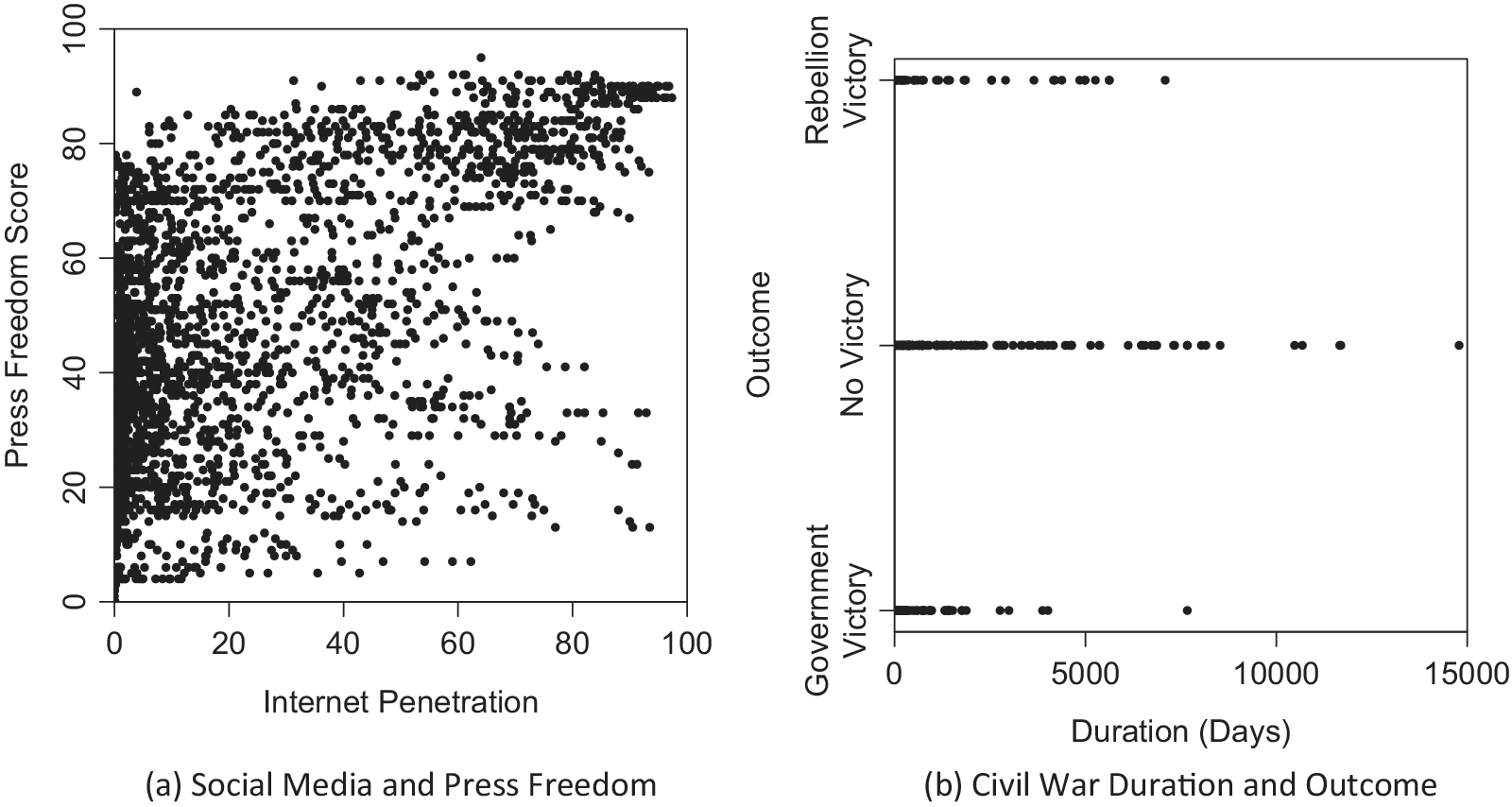
Figure 1 Empirical examples of nonmonotonic dependence. (a) Each dot corresponds to a country in a year, 2000 to 2015 ( $n=2,560$
). (b) Each dot corresponds a civil war, 1946 to 2003 (
$n=2,560$
). (b) Each dot corresponds a civil war, 1946 to 2003 ( $n=267$
).
$n=267$
).
Another instance is civil war duration and outcome, 1946 to 2003 (Cunningham, Gleditsch, and Salehyan Reference Cunningham, Gleditsch and Salehyan2009). In the right panel of Figure 1, each point represents a civil war ( $n=267$
), the horizontal axis indicates the duration in days, and the vertical axis corresponds to the outcome, which is equal to one if the government wins, two if neither side wins, and three if the rebellion wins.Footnote
4
If either the government or the rebellion is strong enough to win, the civil war ends in a short time. Otherwise, neither side obtains a decisive victory, but they instead reach a negotiated settlement to spare the continuing war attrition costs. They do this only after the intrastate military conflict persists for a long duration (Mason, Weingarten Jr, and Fett Reference Mason, Weingarten and Fett1999). Here, the relative power of rebels to governments is a confounder, which is observed but only as a three-category indicator with measurement error.
$n=267$
), the horizontal axis indicates the duration in days, and the vertical axis corresponds to the outcome, which is equal to one if the government wins, two if neither side wins, and three if the rebellion wins.Footnote
4
If either the government or the rebellion is strong enough to win, the civil war ends in a short time. Otherwise, neither side obtains a decisive victory, but they instead reach a negotiated settlement to spare the continuing war attrition costs. They do this only after the intrastate military conflict persists for a long duration (Mason, Weingarten Jr, and Fett Reference Mason, Weingarten and Fett1999). Here, the relative power of rebels to governments is a confounder, which is observed but only as a three-category indicator with measurement error.
In these cases, the underlying copulas have irregular properties, such as nonmonotonicity and asymmetricity. Few parametric copulas can handle these properties. To address this gap, I pay special attention to an overlooked copula (Chesneau Reference Chesneau2021), which I name the “normal mode copula.” It is imperative to enlarge the pool of copulas so that analysts can flexibly adapt the joint distribution to the data and alleviate reliance on the functional-form assumption of the joint distribution (Braumoeller et al. Reference Braumoeller, Marra, Radice and Bradshaw2018).
This article is organized as follows: The next section elaborates on the definition of copulas, introduces some conventional copulas, and defines the normal mode copula. In the following section, I apply these copulas to a dataset on government formation and duration (Chiba et al. Reference Chiba, Martin and Stevenson2015) to demonstrate that the normal mode copula fits the data better than do other conventional copulas. Finally, I present concluding remarks.
2 Definition
2.1 Generic and Gaussian Copulas
Let $0 \leq u_{d} \leq 1$
for
$0 \leq u_{d} \leq 1$
for $d \in \{1, 2\}$
. A function
$d \in \{1, 2\}$
. A function $C(u_{1}, u_{2}): [0, 1]^2 \to [0, 1]$
is called a copula if the following two conditions are met (Nelsen Reference Nelsen2006, 10):
$C(u_{1}, u_{2}): [0, 1]^2 \to [0, 1]$
is called a copula if the following two conditions are met (Nelsen Reference Nelsen2006, 10):
-
Boundary conditions: $C(u_{1}, 0) = C(0, u_{2}) = 0, C(u_{1}, 1) = u_{1}$
, and
$C(1, u_{2}) = u_{2}$
.
$C(u_{1}, 0) = C(0, u_{2}) = 0, C(u_{1}, 1) = u_{1}$
, and
$C(1, u_{2}) = u_{2}$
. -
Two-increasing condition: If
$u_{1}^{L} \leq u_{1}^{H}$
and
$u_{2}^{L} \leq u_{2}^{H}$
, it follows that
$C(u_{1}^{H}, u_{2}^{H}) - C(u_{1}^{L}, u_{2}^{H}) - C(u_{1}^{H}, u_{2}^{L}) + C(u_{1}^{L}, u_{2}^{L}) \geq 0$
.


The motivation for copulas is as follows. I suppose that there are two random variables, $X_{1}$
and
$X_{1}$
and $X_{2}$
. I denote the value of the dth variable
$X_{2}$
. I denote the value of the dth variable $X_{d}$
by
$X_{d}$
by $x_{d}$
, the marginal cumulative distribution function (CDF) of
$x_{d}$
, the marginal cumulative distribution function (CDF) of $X_{d}$
by
$X_{d}$
by $F_{d}(x_{d}) \equiv u_{d}$
, and the joint CDF of
$F_{d}(x_{d}) \equiv u_{d}$
, and the joint CDF of $X_{1}$
and
$X_{1}$
and $X_{2}$
by
$X_{2}$
by $F_{12}(x_{1}, x_{2})$
. Then, according to Sklar’s theorem (Nelsen Reference Nelsen2006, 18 and 24–25), there exists a copula C such that
$F_{12}(x_{1}, x_{2})$
. Then, according to Sklar’s theorem (Nelsen Reference Nelsen2006, 18 and 24–25), there exists a copula C such that
 $$ \begin{align} F_{12}(x_{1}, x_{2}) = C \{ F_{1}(x_{1}), F_{2}(x_{2}) \}. \end{align} $$
When $F_{1}$
and
$F_{1}$
and $F_{2}$
are continuous, C is unique. If
$F_{2}$
are continuous, C is unique. If $X_{1}$
and
$X_{1}$
and $X_{2}$
are continuous variables and we can differentiate both sides of Equation (1) by
$X_{2}$
are continuous variables and we can differentiate both sides of Equation (1) by $x_{1}$
and
$x_{1}$
and $x_{2}$
, we obtain
$x_{2}$
, we obtain
 $$ \begin{align} f_{12}(x_{1}, x_{2}) = f_{1}(x_{1}) f_{2}(x_{2}) c (u_{1}, u_{2}), \end{align} $$
where $f_{d}(x_{d})$
is the probability density function (PDF) of
$f_{d}(x_{d})$
is the probability density function (PDF) of $X_{d}$
and
$X_{d}$
and
 $$ \begin{align*} c (u_{1}, u_{2}) \equiv \frac{\partial^2 }{\partial u_{1} \partial u_{2}} C (u_{1}, u_{2}) \end{align*} $$
represents densities for copula C.Footnote
5
The copula C of $X_{1}$
and
$X_{1}$
and $X_{2}$
abstracts away the marginal distributions of
$X_{2}$
abstracts away the marginal distributions of $X_{1}$
and
$X_{1}$
and $X_{2}$
and thus distills all information about the dependence between
$X_{2}$
and thus distills all information about the dependence between $X_{1}$
and
$X_{1}$
and $X_{2}$
. Equation (2) clarifies the modularity of the copula: we can substitute the marginal distribution of one variable or the copula without changing the other two terms on the right-hand side to obtain a new bivariate distribution on the left-hand side.
$X_{2}$
. Equation (2) clarifies the modularity of the copula: we can substitute the marginal distribution of one variable or the copula without changing the other two terms on the right-hand side to obtain a new bivariate distribution on the left-hand side.
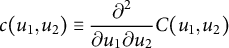
For instance, the Gaussian copula is defined as
 $$ \begin{align*} C_{\mathrm{G}}(u_{1}, u_{2}) \equiv \Phi^2 \{ \Phi^{-1}(u_{1}), \Phi^{-1}(u_{2}) \mid \theta \}, \end{align*} $$
where $\Phi $
and
$\Phi $
and $\Phi ^2$
are univariate and bivariate standard normal distributions, respectively, and
$\Phi ^2$
are univariate and bivariate standard normal distributions, respectively, and $-1 \leq \theta \leq 1$
is the correlation parameter. Figure 2 illustrates an example; the top-left panel shows a contour plot of densities for the joint distribution
$-1 \leq \theta \leq 1$
is the correlation parameter. Figure 2 illustrates an example; the top-left panel shows a contour plot of densities for the joint distribution $f_{12}(x_{1}, x_{2}) = \phi ^2(x_{1}, x_{2} \mid \theta = 0.156)$
, where
$f_{12}(x_{1}, x_{2}) = \phi ^2(x_{1}, x_{2} \mid \theta = 0.156)$
, where $\phi ^2$
is the PDF of
$\phi ^2$
is the PDF of $\Phi ^2$
;Footnote
6
the bottom-left and top-right panels present densities for the marginal distributions
$\Phi ^2$
;Footnote
6
the bottom-left and top-right panels present densities for the marginal distributions $f_{1}(x_{1}) = \phi (x_{1})$
and
$f_{1}(x_{1}) = \phi (x_{1})$
and $f_{2}(x_{2}) = \phi (x_{2})$
, respectively, where
$f_{2}(x_{2}) = \phi (x_{2})$
, respectively, where $\phi $
is the PDF of
$\phi $
is the PDF of $\Phi $
; the bottom-right panel represents a contour plot of densities for the copula
$\Phi $
; the bottom-right panel represents a contour plot of densities for the copula $c(u_{1}, u_{2})$
, which turns to be Gaussian,
$c(u_{1}, u_{2})$
, which turns to be Gaussian, $c_{\mathrm {G}}(u_{1}, u_{2})$
.Footnote
7
If we substitute
$c_{\mathrm {G}}(u_{1}, u_{2})$
.Footnote
7
If we substitute $f_{1}(x_{1}), f_{2}(x_{2})$
, or
$f_{1}(x_{1}), f_{2}(x_{2})$
, or $c (u_{1}, u_{2})$
, the joint distribution
$c (u_{1}, u_{2})$
, the joint distribution $f_{12}(x_{1}, x_{2})$
is no longer represented by
$f_{12}(x_{1}, x_{2})$
is no longer represented by $\phi ^2$
.
$\phi ^2$
.
Figure 2 Bivariate normal distribution: joint distribution, marginal distributions, and copula.
2.2 Conventional Copulas
Scholars have derived dozens of copulas (Hofert et al. Reference Hofert, Kojadinovic, Maechler and Yan2018; Nelsen Reference Nelsen2006; Trivedi and Zimmer Reference Trivedi and Zimmer2007). For reference, I introduce the product copula and the following four conventional copulas: Farlie–Gumbel–Morgenstein (FGM), Ali–Mikhail–Haq (AMH), Clayton, and Frank.
The product (or independence) copula is defined as (Nelsen Reference Nelsen2006, 25)
 $$ \begin{align*} C_{\mathrm{I}} (u_{1}, u_{2}) \equiv u_{1} u_{2}, \end{align*} $$
where $X_{1}$
and
$X_{1}$
and $X_{2}$
are independent of each other.
$X_{2}$
are independent of each other.
The FGM copula is defined as (Nelsen Reference Nelsen2006, 77)
 $$ \begin{align*} C_{\mathrm{FGM}} (u_{1}, u_{2}) \equiv u_{1} u_{2} + \theta u_{1} (1 - u_{1}) u_{2} (1 - u_{2}), \end{align*} $$
where $-1 \leq \theta \leq 1$
.
$-1 \leq \theta \leq 1$
.
The other three belong to a class of Archimedean copulas. Let the generator function $\varphi (u): [0, 1] \to [0, \infty ]$
be a continuous, convex, strictly decreasing function, where
$\varphi (u): [0, 1] \to [0, \infty ]$
be a continuous, convex, strictly decreasing function, where $\varphi (1) = 0$
. I define the pseudoinverse function of
$\varphi (1) = 0$
. I define the pseudoinverse function of $\varphi (u)$
as
$\varphi (u)$
as $\varphi ^{[-1]}(z) = \varphi ^{-1}(z)$
for
$\varphi ^{[-1]}(z) = \varphi ^{-1}(z)$
for $0 \leq z \leq \varphi (0)$
and
$0 \leq z \leq \varphi (0)$
and $\varphi ^{[-1]}(z) = 0$
for
$\varphi ^{[-1]}(z) = 0$
for $\varphi (0) \leq z \leq \infty $
. Then, the following function:
$\varphi (0) \leq z \leq \infty $
. Then, the following function:
 $$ \begin{align*} C_{\mathrm{A}} ( u_{1}, u_{2} \mid \varphi) \equiv \varphi^{[-1]}\{ \varphi(u_{1}) + \varphi(u_{2}) \} \end{align*} $$
meets the two conditions of a copula and is called an Archimedean copula (Nelsen Reference Nelsen2006, 110–112). The generator functions for the AMH, Clayton, and Frank copulas are
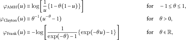 $$ \begin{align*} \varphi_{\mathrm{AMH}}(u) &\equiv \log \left[ \frac{1}{u} \{ 1 - \theta (1 - u) \} \right]& \textrm{for} & \quad -1 \leq \theta \leq 1,\\ \varphi_{\mathrm{Clayton}}(u) &\equiv \theta^{-1} (u^{- \theta} - 1) & \textrm{for} & \quad \theta> 0,\\ \varphi_{\mathrm{Frank}}(u) &\equiv - \log \left[ \frac{1}{\exp( - \theta ) - 1} \{ \exp( - \theta u) - 1 \}\right] & \textrm{for} & \quad \theta \in \mathbb{R},\\ \end{align*} $$
respectively.
Figure 3 shows contour plots of densities for the conventional copulas, where the horizontal and vertical axes are $u_{1}$
and
$u_{1}$
and $u_{2}$
, respectively. Panels correspond to FGM, AMH, Clayton, and Frank.Footnote
8
Clearly, these copulas represent monotonic dependence.
$u_{2}$
, respectively. Panels correspond to FGM, AMH, Clayton, and Frank.Footnote
8
Clearly, these copulas represent monotonic dependence.
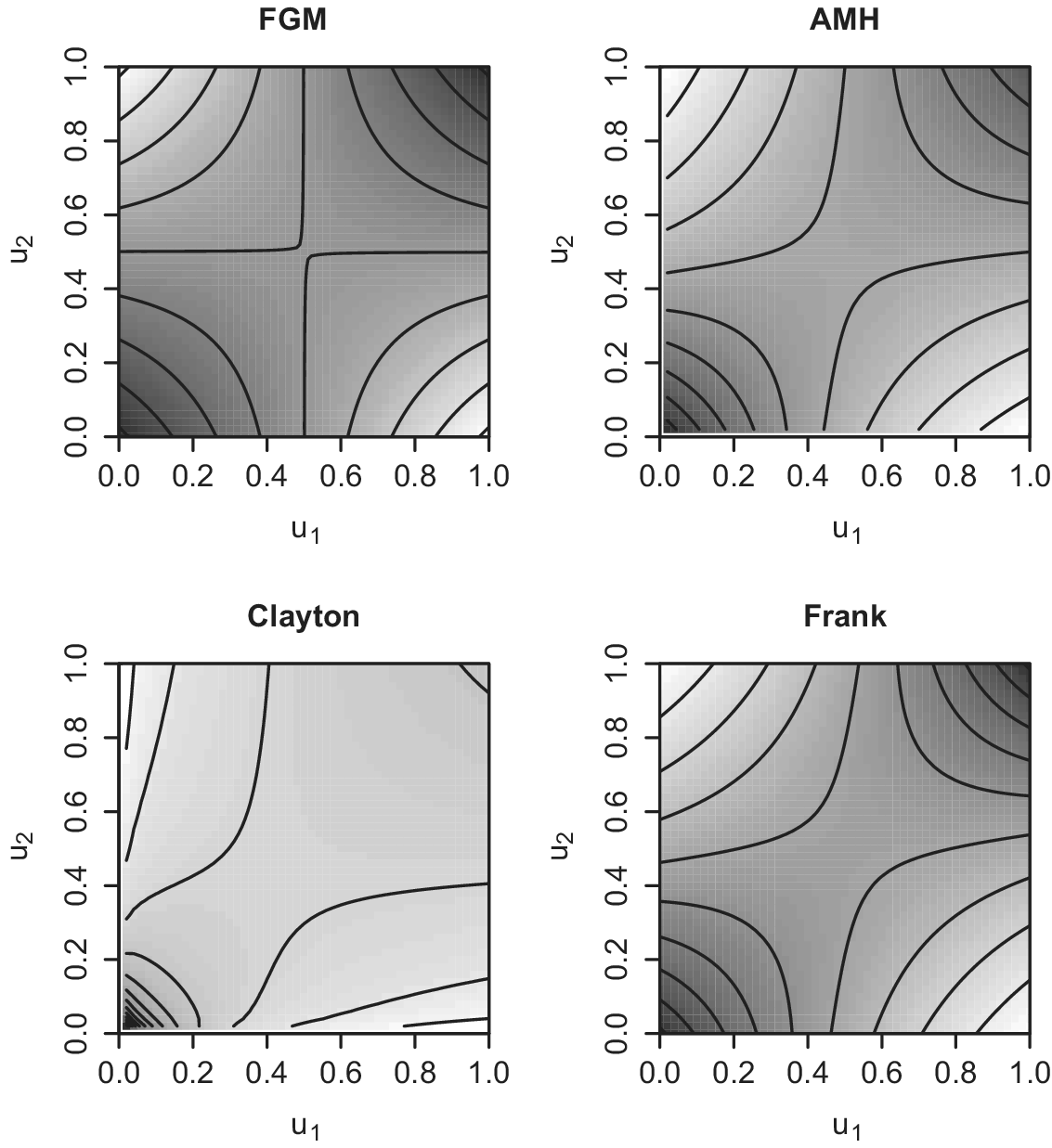
Figure 3 Example plots of conventional copulas.
In general, the three associated copulas of a copula are defined as (Trivedi and Zimmer Reference Trivedi and Zimmer2007, 13–14)
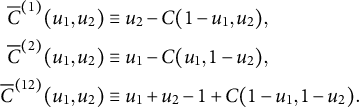 $$ \begin{align} \overline{C}^{(1)} (u_{1}, u_{2}) & \equiv u_{2} - C (1 - u_{1}, u_{2}), \nonumber\\ \overline{C}^{(2)} (u_{1}, u_{2}) & \equiv u_{1} - C (u_{1}, 1 - u_{2}),\\ \overline{C}^{(12)} (u_{1}, u_{2}) & \equiv u_{1} + u_{2} - 1 + C (1 - u_{1}, 1 - u_{2}).\nonumber \end{align} $$
In particular, $\overline {C}^{(12)} (u_{1}, u_{2})$
is called the survival copula (Nelsen Reference Nelsen2006, 32). Figure 4 illustrates contour plots of densities for the associated Clayton copulas. Graphically, by turning the density
$\overline {C}^{(12)} (u_{1}, u_{2})$
is called the survival copula (Nelsen Reference Nelsen2006, 32). Figure 4 illustrates contour plots of densities for the associated Clayton copulas. Graphically, by turning the density $c (u_{1}, u_{2})$
(first panel, the same as the bottom-left panel of Figure 3) with respect to the line
$c (u_{1}, u_{2})$
(first panel, the same as the bottom-left panel of Figure 3) with respect to the line $u_{d} = \frac {1}{2}$
, we obtain
$u_{d} = \frac {1}{2}$
, we obtain $\overline {c}^{(d)} (u_{1}, u_{2})$
(second (
$\overline {c}^{(d)} (u_{1}, u_{2})$
(second ( $d = 1$
) and third (
$d = 1$
) and third ( $d = 2$
) panels); by rotating
$d = 2$
) panels); by rotating $c (u_{1}, u_{2})$
180 degrees, we obtain
$c (u_{1}, u_{2})$
180 degrees, we obtain $\overline {c}^{(12)} (u_{1}, u_{2})$
(fourth panel).Footnote
9
Specifically, I study the three associated copulas for AMH and Clayton copulas (cf. Braumoeller et al. Reference Braumoeller, Marra, Radice and Bradshaw2018, 59); for each of the other conventional copulas, the three associated copulas belong to the family of the original copula.
$\overline {c}^{(12)} (u_{1}, u_{2})$
(fourth panel).Footnote
9
Specifically, I study the three associated copulas for AMH and Clayton copulas (cf. Braumoeller et al. Reference Braumoeller, Marra, Radice and Bradshaw2018, 59); for each of the other conventional copulas, the three associated copulas belong to the family of the original copula.
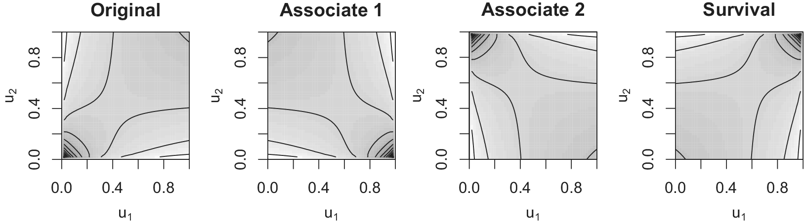
Figure 4 Example plots of associated Clayton copulas.
2.3 Normal Mode Copulas
Chesneau (Reference Chesneau2021) refers to the following copula but only in passing:
 $$ \begin{align} C_{\mathrm{Chesneau}} (u_{1}, u_{2}) = u_{1} u_{2} + \frac{ 1 }{ p_{1} p_{2} \kappa_{1} \kappa_{2} \pi^2 } \theta \{ \sin (u_{1} \kappa_{1} \pi ) \}^{p_{1}} \{ \sin (u_{2} \kappa_{2} \pi ) \}^{p_{2}}, \end{align} $$
where for $d \in \{1, 2\}$
,
$d \in \{1, 2\}$
, $\kappa _{d}$
’s are positive integers,
$\kappa _{d}$
’s are positive integers, $p_{d} \geq 1$
, and
$p_{d} \geq 1$
, and $-1 \leq \theta \leq 1$
.Footnote
10
However, Chesneau (Reference Chesneau2021) did not apply the copula to any real data or give it any name.
$-1 \leq \theta \leq 1$
.Footnote
10
However, Chesneau (Reference Chesneau2021) did not apply the copula to any real data or give it any name.
I simplify this copula by setting $p_{d} = 1$
,
$p_{d} = 1$
,
 $$ \begin{align*} C_{\mathrm{NM}} (u_{1}, u_{2}) \equiv u_{1} u_{2} + \frac{1}{\kappa_{1} \kappa_{2} \pi^2}\theta \sin (u_{1} \kappa_{1} \pi) \sin (u_{2} \kappa_{2} \pi), \end{align*} $$
so that the copula is still flexible in a tractable way with fewer parameters. I name $C_{\mathrm {NM}}$
the normal mode copula,
$C_{\mathrm {NM}}$
the normal mode copula, $\theta $
the amplitude, and
$\theta $
the amplitude, and $\kappa _{d}$
’s mode numbers. (I explain the motivation shortly.)
$\kappa _{d}$
’s mode numbers. (I explain the motivation shortly.)
Figure 5 shows contour plots of densities for normal mode copulas,
 $$ \begin{align*} c_{\mathrm{NM}} (u_{1}, u_{2}) = 1 + \theta \cos (u_{1} \kappa_{1} \pi) \cos (u_{2} \kappa_{2} \pi). \end{align*} $$
The top-left panel corresponds to the case where $\theta = 0.304, \kappa _{1}= 1,$
and
$\theta = 0.304, \kappa _{1}= 1,$
and $\kappa _{2} = 1$
.Footnote
11
This normal mode copula is (radially) symmetric, where
$\kappa _{2} = 1$
.Footnote
11
This normal mode copula is (radially) symmetric, where $U_{2}$
monotonically increases in
$U_{2}$
monotonically increases in $U_{1}$
. In the top-right panel, I present another normal mode copula where I only change
$U_{1}$
. In the top-right panel, I present another normal mode copula where I only change $\theta $
from
$\theta $
from $0.304$
to
$0.304$
to $-0.304$
. We obtain the current plot by making the dark parts in the previous plot light and vice versa. Here,
$-0.304$
. We obtain the current plot by making the dark parts in the previous plot light and vice versa. Here, $U_{2}$
monotonically decreases in
$U_{2}$
monotonically decreases in $U_{1}$
. The bottom-left panel represents the case where
$U_{1}$
. The bottom-left panel represents the case where $\theta = 0.304, \kappa _{1}= 2,$
and
$\theta = 0.304, \kappa _{1}= 2,$
and $\kappa _{2} = 1$
. This normal mode copula is not (radially) symmetric. Moreover,
$\kappa _{2} = 1$
. This normal mode copula is not (radially) symmetric. Moreover, $U_{2}$
monotonically increases in
$U_{2}$
monotonically increases in $U_{1}$
for
$U_{1}$
for $U_{1} \leq \frac {1}{2}$
but decreases in
$U_{1} \leq \frac {1}{2}$
but decreases in $U_{1}$
for
$U_{1}$
for $U_{1} \geq \frac {1}{2}$
. Thus, the copula represents a case of nonmonotonic dependence that motivates me, as I explained in Section 1. In fact, if we rotate the plot clockwise (counterclockwise) 90 degrees, it resembles the right (left) panel of Figure 1. Finally, the bottom-right panel addresses the case where
$U_{1} \geq \frac {1}{2}$
. Thus, the copula represents a case of nonmonotonic dependence that motivates me, as I explained in Section 1. In fact, if we rotate the plot clockwise (counterclockwise) 90 degrees, it resembles the right (left) panel of Figure 1. Finally, the bottom-right panel addresses the case where $\theta = 0.304, \kappa _{1}= 2,$
and
$\theta = 0.304, \kappa _{1}= 2,$
and $\kappa _{2} = 2$
. This normal mode copula is (radially) symmetric but has nonmonotonic dependence.
$\kappa _{2} = 2$
. This normal mode copula is (radially) symmetric but has nonmonotonic dependence.
Figure 5 Example plots of normal mode copulas.
If we regard $u_{1}$
as the position along an open pipe (such as a flute) with unit length and
$u_{1}$
as the position along an open pipe (such as a flute) with unit length and $u_{2}$
as time, the displacement of a standing sound wave with one frequency at position
$u_{2}$
as time, the displacement of a standing sound wave with one frequency at position $u_{1}$
and time
$u_{1}$
and time $u_{2}$
resembles
$u_{2}$
resembles $c_{\mathrm {NM}} (u_{1}, u_{2})$
.Footnote
12
Importantly, if
$c_{\mathrm {NM}} (u_{1}, u_{2})$
.Footnote
12
Importantly, if $\kappa _{1}$
were not an integer, the corresponding sound wave would not form a standing wave and would not resonate, thus dissipating immediately. In general, this kind of standing wave is called the normal mode. This is why I name
$\kappa _{1}$
were not an integer, the corresponding sound wave would not form a standing wave and would not resonate, thus dissipating immediately. In general, this kind of standing wave is called the normal mode. This is why I name $C_{\mathrm {NM}}$
the normal mode copula.
$C_{\mathrm {NM}}$
the normal mode copula.
3 Application
3.1 Overview
This section intends to showcase the usefulness of normal mode copulas by reanalyzing Chiba et al. (Reference Chiba, Martin and Stevenson2015, hereafter, “CMS”), who also use a copula.Footnote 13 CMS focus on two outcomes of (coalition) government formation and duration. Scholars have studied what factors affect either outcome. One problem is that these two outcomes are interrelated, and failure to consider simultaneity leads to selection bias in estimating the model. For instance, if a government would not remain in power for a long time, say, due to a hidden scandal, it may be less likely to be formed in the first place. If (and probably as) scholars do not observe all confounders (e.g., the hidden scandal) that affect both outcomes or do observe some of them but with measurement error, the resultant estimates will be less efficient and might suffer from omitted variable bias. To address this problem, CMS incorporate a copula into their model and analyze the two outcomes jointly. A remaining concern is that CMS consider only the Gaussian copula. I substitute the normal mode copulas as well as other conventional copulas to show that a normal mode copula is the best.
3.2 Model
To focus on the comparison between the Gaussian copula and other copulas, this subsection introduces a simplified version of the CMS model using my notation.Footnote
14
The units of observation are a (coalition government) formation opportunity $i \in \{1,2,\ldots ,n = 432\}$
and a potential coalition government (combination of parties)
$i \in \{1,2,\ldots ,n = 432\}$
and a potential coalition government (combination of parties) $j \in \mathcal {J}_{i} \equiv \{1,2,\ldots ,m_{i}\}$
(
$j \in \mathcal {J}_{i} \equiv \{1,2,\ldots ,m_{i}\}$
( $\sum _{i} m_{i} = 95,576$
). For each i, we have two outcome variables. The first outcome is a realized government,
$\sum _{i} m_{i} = 95,576$
). For each i, we have two outcome variables. The first outcome is a realized government, $Y_{1, i} \in \mathcal {J}_{i}$
. The second outcome is the duration of the government from its inception to its termination,
$Y_{1, i} \in \mathcal {J}_{i}$
. The second outcome is the duration of the government from its inception to its termination, $Y_{2, i} \in (0, \bar {y}_{i}]$
, where
$Y_{2, i} \in (0, \bar {y}_{i}]$
, where $\bar {y}_{i}$
is the constitutional interelection period. Unless a government ends for political reasons (replacement by another government without an election or dissolution of the legislature followed by an early election), I regard the government’s duration as censored.Footnote
15
$\bar {y}_{i}$
is the constitutional interelection period. Unless a government ends for political reasons (replacement by another government without an election or dissolution of the legislature followed by an early election), I regard the government’s duration as censored.Footnote
15
CMS use a conditional logit model to explain government formation. We denote a covariate vector by $\boldsymbol {z}_{1, ij}$
and the corresponding coefficient vector by
$\boldsymbol {z}_{1, ij}$
and the corresponding coefficient vector by $\boldsymbol {\theta }_{1}$
. Specifically,
$\boldsymbol {\theta }_{1}$
. Specifically, $\boldsymbol {z}_{1, ij}$
is composed of Minority Government, Status Quo Government, and dozens of party dummy variables.Footnote
16
The probability that government
$\boldsymbol {z}_{1, ij}$
is composed of Minority Government, Status Quo Government, and dozens of party dummy variables.Footnote
16
The probability that government $g \in \mathcal {J}_{i}$
is formed is modeled as
$g \in \mathcal {J}_{i}$
is formed is modeled as
 $$ \begin{align*} \Pr(Y_{1, i} = g) & = \frac{\exp(\boldsymbol{z}^{\prime}_{1, ig} \boldsymbol{\theta}_{1})}{\sum_{j \in \mathcal{J}_{i}} \exp(\boldsymbol{z}^{\prime}_{1, ij} \boldsymbol{\theta}_{1})} \\ & \equiv G(g \mid \boldsymbol{z}_{1, i}, \boldsymbol{\theta}_{1}), \end{align*} $$
where $\boldsymbol {z}_{1, i} \equiv (\boldsymbol {z}_{1, i1}^{\prime }, \boldsymbol {z}_{1, i2}^{\prime }, \ldots , \boldsymbol {z}_{1, i m_{i}}^{\prime })^{\prime }$
. In my understanding, CMS implicitly assume that when a latent utility variable
$\boldsymbol {z}_{1, i} \equiv (\boldsymbol {z}_{1, i1}^{\prime }, \boldsymbol {z}_{1, i2}^{\prime }, \ldots , \boldsymbol {z}_{1, i m_{i}}^{\prime })^{\prime }$
. In my understanding, CMS implicitly assume that when a latent utility variable $X_{1, i}$
is smaller than
$X_{1, i}$
is smaller than $\overline {x}_{1, i} \equiv F_{1}^{-1} \{G(g \mid \boldsymbol {z}_{1, i}, \boldsymbol {\theta }_{1})\}$
, we observe
$\overline {x}_{1, i} \equiv F_{1}^{-1} \{G(g \mid \boldsymbol {z}_{1, i}, \boldsymbol {\theta }_{1})\}$
, we observe $Y_{1, i} = g$
.Footnote
17
$Y_{1, i} = g$
.Footnote
17
CMS’s main model assumes that the government duration follows a Weibull distribution, $F_{2}(t \mid \theta _{2, \mathrm {inv.scale}}, \theta _{2, \mathrm {shape}})$
, where
$F_{2}(t \mid \theta _{2, \mathrm {inv.scale}}, \theta _{2, \mathrm {shape}})$
, where $\theta _{2, \mathrm {inv.scale}}$
is the inverse scale parameter and
$\theta _{2, \mathrm {inv.scale}}$
is the inverse scale parameter and $\theta _{2, \mathrm {shape}}$
is the shape parameter. We denote the latent time variable by
$\theta _{2, \mathrm {shape}}$
is the shape parameter. We denote the latent time variable by $X_{2, i}$
, another covariate vector by
$X_{2, i}$
, another covariate vector by $\boldsymbol {z}_{2, i}$
, and the corresponding coefficient vector by
$\boldsymbol {z}_{2, i}$
, and the corresponding coefficient vector by $\boldsymbol {\theta }_{2, \mathrm {coef}}$
. To be concrete, I include Minority and Polarization Index in
$\boldsymbol {\theta }_{2, \mathrm {coef}}$
. To be concrete, I include Minority and Polarization Index in $\boldsymbol {z}_{2, i}$
.Footnote
18
The probability density that the length of the duration is t is modeled as
$\boldsymbol {z}_{2, i}$
.Footnote
18
The probability density that the length of the duration is t is modeled as
 $$ \begin{align*} p(X_{2, i} = t) = f_{2}(t \mid \theta_{2, \mathrm{inv.scale}}, \theta_{2, \mathrm{shape}}), \end{align*} $$
where $\theta _{2, \mathrm {inv.scale}} = \exp (- \boldsymbol {z}^{\prime }_{2, i} \boldsymbol {\theta }_{2, \mathrm {coef}})$
.
$\theta _{2, \mathrm {inv.scale}} = \exp (- \boldsymbol {z}^{\prime }_{2, i} \boldsymbol {\theta }_{2, \mathrm {coef}})$
.
Let $W_{i}$
be the censoring indicator. If the duration ends for political reasons at
$W_{i}$
be the censoring indicator. If the duration ends for political reasons at $t < \bar {y}_{i}$
, we observe
$t < \bar {y}_{i}$
, we observe $W_{i} = 0$
,
$W_{i} = 0$
, $Y_{1, i} = g$
, and
$Y_{1, i} = g$
, and $Y_{2, i} = X_{2, i} = t$
, and the mixed joint density is
$Y_{2, i} = X_{2, i} = t$
, and the mixed joint density is
 $$ \begin{align} p(Y_{1, i} = g, Y_{2, i} = t) & = \Pr ( X_{1, i} \leq \overline{x}_{1, i} \mid X_{2, i} = t ) p(X_{2, i} = t) \nonumber\\ & = F_{1 \mid 2}( \overline{x}_{1, i} \mid X_{2, i} = t) f_{2}(t \mid \boldsymbol{z}_{2, i}, \boldsymbol{\theta}_{2}) \\ & = C^{\prime}_{1 \mid 2} ( \overline{u}_{1, i} \mid \underline{u}_{2, i}, \theta_{12}) f_{2}(t \mid \boldsymbol{z}_{2, i}, \boldsymbol{\theta}_{2}),\nonumber \end{align} $$
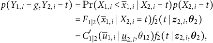
where $\overline {u}_{1, i} = F_{1}(\overline {x}_{1, i}) = G(g \mid \boldsymbol {z}_{1, i}, \boldsymbol {\theta }_{1})$
,
$\overline {u}_{1, i} = F_{1}(\overline {x}_{1, i}) = G(g \mid \boldsymbol {z}_{1, i}, \boldsymbol {\theta }_{1})$
, $\underline {u}_{2, i} \equiv F_{2}(t \mid \boldsymbol {z}_{2, i}, \boldsymbol {\theta }_{2})$
,
$\underline {u}_{2, i} \equiv F_{2}(t \mid \boldsymbol {z}_{2, i}, \boldsymbol {\theta }_{2})$
, $\boldsymbol {\theta }_{2} \equiv (\boldsymbol {\theta }_{2, \mathrm {coef}}^{\prime }, \theta _{2, \mathrm {shape}})^{\prime }$
,
$\boldsymbol {\theta }_{2} \equiv (\boldsymbol {\theta }_{2, \mathrm {coef}}^{\prime }, \theta _{2, \mathrm {shape}})^{\prime }$
, $\theta _{12}$
is the parameter of copula C of
$\theta _{12}$
is the parameter of copula C of $X_{1}$
and
$X_{1}$
and $X_{2}$
, and it generally holds that
$X_{2}$
, and it generally holds that $\Pr (X_{1} \leq x_{1} \mid X_{2} = x_{2}) = \frac {\partial }{\partial u_{2}} C (u_{1}, u_{2}) \equiv C^{\prime }_{1 \mid 2} ( u_{1} \mid u_{2})$
(Nelsen Reference Nelsen2006, 41).
$\Pr (X_{1} \leq x_{1} \mid X_{2} = x_{2}) = \frac {\partial }{\partial u_{2}} C (u_{1}, u_{2}) \equiv C^{\prime }_{1 \mid 2} ( u_{1} \mid u_{2})$
(Nelsen Reference Nelsen2006, 41).
If the duration is censored at t, we observe $W_{i} = 1$
,
$W_{i} = 1$
, $Y_{1, i} = g$
, and
$Y_{1, i} = g$
, and $Y_{2, i} = t$
but not
$Y_{2, i} = t$
but not $X_{2, i}> t$
, and the joint probability is
$X_{2, i}> t$
, and the joint probability is
 $$ \begin{align} \Pr(Y_{1, i} = g, Y_{2, i} = t) & = \Pr(X_{1, i} \leq \overline{x}_{1, i}, X_{2, i}> t) \nonumber\\ & = \Pr(X_{1, i} \leq \overline{x}_{1, i}) - \Pr(X_{1, i} \leq \overline{x}_{1, i}, X_{2, i} \leq t) \\ & = F_{1}(\overline{x}_{1, i}) - F_{12}(\overline{x}_{1, i}, t) \nonumber\\ & = \overline{u}_{1, i} - C ( \overline{u}_{1, i}, \underline{u}_{2, i}\mid \theta_{12}).\nonumber \end{align} $$
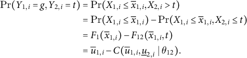
By multiplying either Equation (5) or (6), we can obtain the total likelihood function,
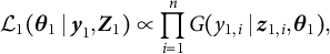
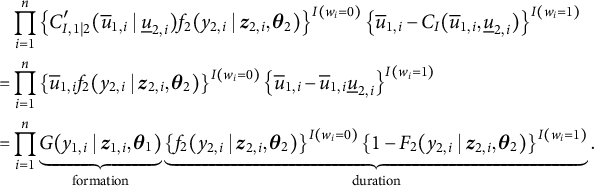
 $$\begin{align} \mathcal{L}_{12} ( \boldsymbol{\theta}_{1}, \boldsymbol{\theta}_{2}, \theta_{12} \mid \boldsymbol{w}, \boldsymbol{y}_{1}, \boldsymbol{y}_{2}, \boldsymbol{Z}_{1}, \boldsymbol{Z}_{2}) \propto & \prod^{n}_{i = 1} \left\{ C^{\prime}_{1 \mid 2} ( \overline{u}_{1, i} \mid \underline{u}_{2, i}, \theta_{12}) f_{2}(y_{2, i} \mid \boldsymbol{z}_{2, i}, \boldsymbol{\theta}_{2})\right\}^{I(w_{i} = 0)} \\ & \left\{ \overline{u}_{1, i} - C ( \overline{u}_{1, i}, \underline{u}_{2, i}\mid \theta_{12}) \right\}^{I(w_{i} = 1)},\nonumber \end{align}$$
where $I(\cdot )$
is the dummy indicator function, and maximize it to estimate the parameters,
$I(\cdot )$
is the dummy indicator function, and maximize it to estimate the parameters, $\boldsymbol {\theta }_{1}, \boldsymbol {\theta }_{2}$
, and
$\boldsymbol {\theta }_{1}, \boldsymbol {\theta }_{2}$
, and $\theta _{12}$
. This is the CMS model.
$\theta _{12}$
. This is the CMS model.
3.3 Studied Copulas
CMS assume that the copula of $X_{1}$
and
$X_{1}$
and $X_{2}$
is a Gaussian copula. My departure from the CMS model starts here. I substitute normal mode copulas. In general, before analysts apply a normal mode copula to any dataset, they have to determine the values of
$X_{2}$
is a Gaussian copula. My departure from the CMS model starts here. I substitute normal mode copulas. In general, before analysts apply a normal mode copula to any dataset, they have to determine the values of $\kappa _{1}$
and
$\kappa _{1}$
and $\kappa _{2}$
, which are model choice indicators rather than parameters to be estimated. In my case, I explore
$\kappa _{2}$
, which are model choice indicators rather than parameters to be estimated. In my case, I explore $\kappa _{1}, \kappa _{2} \in \{1,2,3,4\}$
. I also consider the following four conventional copulas: FGM, AMH, Clayton, and Frank. The three associated copulas of AMH and Clayton copulas are also studied.
$\kappa _{1}, \kappa _{2} \in \{1,2,3,4\}$
. I also consider the following four conventional copulas: FGM, AMH, Clayton, and Frank. The three associated copulas of AMH and Clayton copulas are also studied.
For the purpose of comparison, I analyze the “separate” model of formation and duration by maximizing each of the following likelihood functions:
 $$\begin{align} \mathcal{L}_{1} ( \boldsymbol{\theta}_{1} \mid \boldsymbol{y}_{1}, \boldsymbol{Z}_{1}) & \propto \prod^{n}_{i = 1} G(y_{1, i} \mid \boldsymbol{z}_{1, i}, \boldsymbol{\theta}_{1}),\quad\quad\qquad\qquad\qquad\qquad\qquad\qquad \end{align}$$
 $$\begin{align} \mathcal{L}_{2} ( \boldsymbol{\theta}_{2} \mid \boldsymbol{w}, \boldsymbol{y}_{2}, \boldsymbol{Z}_{2}) & \propto \prod^{n}_{i = 1} \left\{ f_{2}(y_{2, i} \mid \boldsymbol{z}_{2, i}, \boldsymbol{\theta}_{2}) \right\}^{I(w_{i} = 0)} \left\{ 1 - F_{2}(y_{2, i} \mid \boldsymbol{z}_{2, i}, \boldsymbol{\theta}_{2}) \right\}^{I(w_{i} = 1)}. \end{align}$$
I also analyze another duration model where I include the predicted probability of formation ( $\hat {\overline {u}}_{1, i}$
, hereafter, “Formation Probability”), which is estimated by using the formation model (Equation (8)), as a covariate:
$\hat {\overline {u}}_{1, i}$
, hereafter, “Formation Probability”), which is estimated by using the formation model (Equation (8)), as a covariate:
 $$\begin{align} \mathcal{L}^{*}_{2} ( \boldsymbol{\theta}^{*}_{2} \mid \boldsymbol{w}, \boldsymbol{y}_{2}, \boldsymbol{Z}_{2}, {\hat{\overline{\boldsymbol{u}}}_{1}}) \propto \prod^{n}_{i = 1} \left\{ f_{2}(y_{2, i} \mid \boldsymbol{z}_{2, i}, \hat{\overline{u}}_{1, i}, \boldsymbol{\theta}^{*}_{2}) \right\}^{I(w_{i} = 0)} \left\{ 1 - F_{2}(y_{2, i} \mid \boldsymbol{z}_{2, i}, \hat{\overline{u}}_{1, i}, \boldsymbol{\theta}^{*}_{2}) \right\}^{I(w_{i} = 1)}. \end{align}$$
If the relationship between formation and duration is monotonic, this “two-step” model should work.Footnote
19
Note that the separate and two-step models are effectively equivalent to the CMS model with the product copula ( $C_{I}$
), which has no parameter, because
$C_{I}$
), which has no parameter, because $C^{\prime }_{I, 1 \mid 2} (u_{1} \mid u_{2}) = u_{1}$
and Equation (7) becomes
$C^{\prime }_{I, 1 \mid 2} (u_{1} \mid u_{2}) = u_{1}$
and Equation (7) becomes
 $$ \begin{align*} & \prod^{n}_{i = 1} \left\{ C^{\prime}_{I, 1 \mid 2} ( \overline{u}_{1, i} \mid \underline{u}_{2, i}) f_{2}(y_{2, i} \mid \boldsymbol{z}_{2, i}, \boldsymbol{\theta}_{2})\right\}^{I(w_{i} = 0)} \left\{ \overline{u}_{1, i} - C_{I} ( \overline{u}_{1, i}, \underline{u}_{2, i}) \right\}^{I(w_{i} = 1)} \\ =& \prod^{n}_{i = 1} \left\{ \overline{u}_{1, i} f_{2}(y_{2, i} \mid \boldsymbol{z}_{2, i}, \boldsymbol{\theta}_{2})\right\}^{I(w_{i} = 0)} \left\{ \overline{u}_{1, i} - \overline{u}_{1, i} \underline{u}_{2, i} \right\}^{I(w_{i} = 1)} \\ =& \prod^{n}_{i = 1} \underbrace{G(y_{1, i} \mid \boldsymbol{z}_{1, i}, \boldsymbol{\theta}_{1})}_{\textrm{formation}} \underbrace{\left\{ f_{2}(y_{2, i} \mid \boldsymbol{z}_{2, i}, \boldsymbol{\theta}_{2})\right\}^{I(w_{i} = 0)} \left\{ 1 - F_{2}(y_{2, i} \mid \boldsymbol{z}_{2, i}, \boldsymbol{\theta}_{2})\right\}^{I(w_{i} = 1)}}_{\textrm{duration}}. \end{align*} $$
If copula models improve the model fit, we can alleviate bias due to unobserved confounders and root mean squared error (CMS, Braumoeller et al. Reference Braumoeller, Marra, Radice and Bradshaw2018). I also expect that a copula model that fits the data better leads to smaller standard errors because the copula model takes greater advantage of the information about formation ( $X_{1}$
) in estimating the parameters about duration (
$X_{1}$
) in estimating the parameters about duration ( $X_{2}$
), and thus the conditional variance of duration given formation is smaller.
$X_{2}$
), and thus the conditional variance of duration given formation is smaller.
3.4 Results
Table 1 reports the Akaike information criterion (AIC) for each copula used in the CMS model.Footnote
20
Each row indicates the model with each copula. In the first and second rows, I report the AICs of the separate and two-step models, respectively, where I sum the AICs of the formation model (Equation (8)) and the duration model (Equation (9) for the separate model and Equation (10) for the two-step model). The AIC of the two-step model is larger than that of the separate model almost by two, which means the predicted probability of formation has little linear relation with duration. Below, all models employ Equation (7). Compared with the separate model, the Gaussian copula model CMS used (third row) worsens the AIC. In the next 16 rows, I display the AICs of normal mode copula models. The normal mode copula model with $\kappa _{1} = 1$
and
$\kappa _{1} = 1$
and $\kappa _{2} = 2$
(hereafter, the “NM(1, 2) copula model,” fifth row) has the best (i.e., smallest) AIC. In the last ten rows, I present the AICs of the conventional copula models and their associated copula models. (For the AMH and Clayton copulas, “Original,” “Associate 1,” “Associate 2,” and “Survival” indicate C,
$\kappa _{2} = 2$
(hereafter, the “NM(1, 2) copula model,” fifth row) has the best (i.e., smallest) AIC. In the last ten rows, I present the AICs of the conventional copula models and their associated copula models. (For the AMH and Clayton copulas, “Original,” “Associate 1,” “Associate 2,” and “Survival” indicate C, $\overline {C}^{(1)}$
,
$\overline {C}^{(1)}$
, $\overline {C}^{(2)}$
, and
$\overline {C}^{(2)}$
, and $\overline {C}^{(12)}$
(Equation (3)), respectively.) They have almost the same AIC as the two-step model and do not outperform the NM(1, 2) copula model. This is probably because all of these conventional copulas cope with monotonic relationships alone, where in fact, the relation between
$\overline {C}^{(12)}$
(Equation (3)), respectively.) They have almost the same AIC as the two-step model and do not outperform the NM(1, 2) copula model. This is probably because all of these conventional copulas cope with monotonic relationships alone, where in fact, the relation between $\overline {u}_{1, i}$
and
$\overline {u}_{1, i}$
and $\underline {u}_{2, i}$
is nonmonotonic as shown next.
$\underline {u}_{2, i}$
is nonmonotonic as shown next.
Table 1 AICs for models using various copulas.
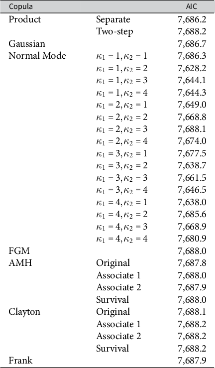
Figure 6 illustrates the scatter plots of estimated $\overline {u}_{1, i}$
’s (horizontal axis) and
$\overline {u}_{1, i}$
’s (horizontal axis) and $\underline {u}_{2, i}$
’s (vertical axis). The left and right panels correspond to the Gaussian copula model and the NM(1, 2) copula model, respectively. In each panel, the contour plot of the copula based on the estimate of
$\underline {u}_{2, i}$
’s (vertical axis). The left and right panels correspond to the Gaussian copula model and the NM(1, 2) copula model, respectively. In each panel, the contour plot of the copula based on the estimate of $\theta _{12}$
is overlaid.Footnote
21
A point indicates a unit that is not censored, where
$\theta _{12}$
is overlaid.Footnote
21
A point indicates a unit that is not censored, where $(U_{1, i}, U_{2, i}) \in \{ (u_{1}, u_{2}) \mid 0 < u_{1} \leq \overline {u}_{1, i}, u_{2} = \underline {u}_{2, i} \}$
. A cross indicates a unit that is censored, where
$(U_{1, i}, U_{2, i}) \in \{ (u_{1}, u_{2}) \mid 0 < u_{1} \leq \overline {u}_{1, i}, u_{2} = \underline {u}_{2, i} \}$
. A cross indicates a unit that is censored, where $(U_{1, i}, U_{2, i}) \in \{ (u_{1}, u_{2}) \mid 0 < u_{1} \leq \overline {u}_{1, i}, \underline {u}_{2, i} < u_{2} < 1 \}$
. Clearly, the relationship between
$(U_{1, i}, U_{2, i}) \in \{ (u_{1}, u_{2}) \mid 0 < u_{1} \leq \overline {u}_{1, i}, \underline {u}_{2, i} < u_{2} < 1 \}$
. Clearly, the relationship between $\overline {u}_{1, i}$
and
$\overline {u}_{1, i}$
and $\underline {u}_{2, i}$
is nonmonotonic. Since I use a simplified CMS model, neither copula model appears to fit the data well. However, units near the right vertical axis are situated in low-density areas of the Gaussian copula model but in high-density areas of the NM(1, 2) copula model. This is likely why the NM(1, 2) copula model achieves the best performance among the studied copulas in Table 1.
$\underline {u}_{2, i}$
is nonmonotonic. Since I use a simplified CMS model, neither copula model appears to fit the data well. However, units near the right vertical axis are situated in low-density areas of the Gaussian copula model but in high-density areas of the NM(1, 2) copula model. This is likely why the NM(1, 2) copula model achieves the best performance among the studied copulas in Table 1.
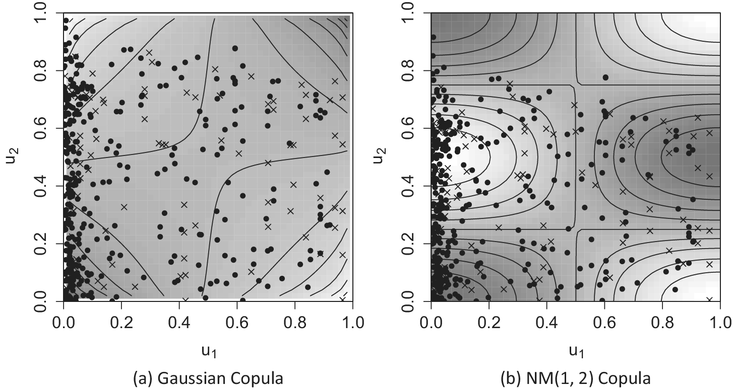
Figure 6 Scatter plots of ${\overline{u}}_{1, i}$
’s and
${\overline{u}}_{1, i}$
’s and ${\underline{u}}_{2, i}$
’s with contour plots of the estimated copula.
${\underline{u}}_{2, i}$
’s with contour plots of the estimated copula. $n = 432$
.
$n = 432$
.
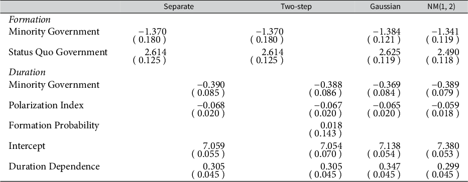
Table 2 presents the estimation results of the parameters.Footnote
22
The first two rows display covariate coefficients of the formation model ( $\boldsymbol {\theta }_{1}$
except for dozens of party fixed effects). The third to sixth rows indicate covariate coefficients of the duration model (including intercept,
$\boldsymbol {\theta }_{1}$
except for dozens of party fixed effects). The third to sixth rows indicate covariate coefficients of the duration model (including intercept, $\boldsymbol {\theta }_{2, \mathrm {coef}}$
), while the last row represents the logged shape parameter of the duration model (
$\boldsymbol {\theta }_{2, \mathrm {coef}}$
), while the last row represents the logged shape parameter of the duration model ( $\log (\theta _{\mathrm {shape}})$
). The first and second columns concern the separate model (Equations (8) and (9), respectively), while the third and fourth columns correspond to the two-step model (Equations (8) and (10), respectively; thus, the first column is the same as the third column). In the fifth and sixth columns, I show the results of the Gaussian copula model and the NM(1, 2) copula model, respectively (Equation (7)). In each cell, the entry is the estimate with the standard error in parentheses.
$\log (\theta _{\mathrm {shape}})$
). The first and second columns concern the separate model (Equations (8) and (9), respectively), while the third and fourth columns correspond to the two-step model (Equations (8) and (10), respectively; thus, the first column is the same as the third column). In the fifth and sixth columns, I show the results of the Gaussian copula model and the NM(1, 2) copula model, respectively (Equation (7)). In each cell, the entry is the estimate with the standard error in parentheses.
Table 2 Results of parameter estimation.
Note: Cell entries are estimates (with standard errors in parentheses). $n = 432$
.
$n = 432$
.
As expected, all standard errors are smaller in the NM(1, 2) copula model than in the separate model, the two-step model, and the Gaussian copula model, except for that of the Duration Dependence parameter. In the case of Minority Government as a formation covariate, the standard error of the NM(1, 2) copula model is reduced by 34% compared with that of the separate model. The coefficient of Formation Probability in the two-step model is close to zero and not significant, although the NM(1, 2) copula model performs well. (Recall also that the two-step model does not improve the AIC compared with the separate model in Table 1.) This implies that the probability of formation affects duration not in a monotonic way but in a nonmonotonic way. Point estimates are not particularly different across models in the simplified models. However, if I use the full CMS model, they are so distinct that coefficient estimates are statistically significantly different from zero in one model but not in another (Supplementary Material).
4 Conclusion
This study sheds light on an understudied family of copulas, normal mode copulas. I apply dozens of copulas to a dataset of government formation and duration to show that the normal mode copula achieves higher performance than other conventional copulas.
There are several directions for future research. In a companion paper (Fukumoto Reference Fukumoto2023a), I have characterized the properties of normal mode copulas such as monotonicity and measures of association. It is also promising to explore the properties of Chesneau’s (Reference Chesneau2021) copulas (Equation (4)) and its multivariate version. Scholars can apply normal mode copulas to various data to find interesting dependence structures. I hope normal mode copulas become a helpful tool to analyze mutually dependent variables in political science.
Acknowlegments
Earlier versions of this article were presented on November 5, 2013, June 23, 2015, and September 16, 2022, at the Institute of Statistical Mathematics, Tokyo, Japan, and on January 6–7, 2023, at the 10th Asian Political Methodology Meeting, National University of Singapore. I thank Toshikazu Kitano and Dean Knox for their helpful comments. I am grateful to Korhan Kocak, Özgür Kıbrıs, David E. Cunningham, Kristian Skrede Gleditsch, Idean Salehyan, Daina Chiba, Lanny W. Martin, and Randolph T. Stevenson for enabling me to reanalyze their datasets. I also appreciate American Journal Experts for providing proofreading service. I am entirely responsible for the scientific content of the article, and the article adheres to the journal’s authorship policy.
Funding
This work was supported by the Japan Society for the Promotion of Science (Grant No. KAKENHI JP19K21683) and the Gakushuin University's Computer Centre (no grant number).
Conflicts of Interest
There are no conflicts of interest to disclose.
Data Availability Statement
The replication materials for this article can be found in Fukumoto (Reference Fukumoto2023b) at https://doi.org/10.7910/DVN/X94ITA.
Supplementary Material
For supplementary material accompanying this paper, please visit https://doi.org/10.1017/pan.2023.45.


 Open access