2 What Exactly is Measured?

The kurtosis (k) is defined as the fourth moment of a distribution. Contrary to the first three moments (mean, variance, and skewness), the interpretation of k is the object of debate. It is often wrongly interpreted as the peakedness of a distribution. This interpretation has been common in political science and among statisticians, even though research pointed out for a long time that the kurtosis of a given distribution and its peakedness do not necessarily align with each other (Kaplansky Reference Kaplansky1945). If anything, k can be seen as a measure for the tailedness of a distribution (Westfall Reference Westfall2014). This becomes clear when looking at the standardized measure of k for a random variable X which is defined as:

(1) $$ \begin{align} k = E(Z^4), \end{align} $$

(2) $$ \begin{align} Z = \frac{X-E(X).}{\sigma_X} \end{align} $$

This definition allows for an intuitive interpretation of why k only concerns the tails. Z is defined as the difference between the observed value X and its expected value $E(X)$ divided by the standard deviation $\sigma _X$ . Therefore, the Z-score indicates the number of standard deviations separating a value from its expected value. Therefore, outliers with high Z-scores, heavily influence the value of k while values around 0 have nearly no influence. To somewhat alleviate this problem, the literature moved forward using moments that are based on L-statistics (Hosking Reference Hosking1990). L-moments build on the linear combination of order statistics, where $X_{k:r}$ is is the kth smallest observation in a sample of the size r. The L-kurtosis ( $\tau _4$ ) is defined as the ratio of the fourth ( $\lambda _4$ ) and the second L-moment ( $\lambda _2$ ):

(3) $$ \begin{align} \tau_4 = \frac{\lambda_4}{\lambda_2} \end{align} $$

$\lambda _2$ represents a measure of scale and is defined as the expected difference of two randomly drawn values (X) from a given distribution:

(4) $$ \begin{align} \lambda_2 = \frac{1}{2}E(X_{2:2} - X_{1:2}). \end{align} $$

The definition of $\lambda _4$ is more complicated. It is defined as the “central third difference of the expected order statistic of a sample of the size 4” (Hosking Reference Hosking1990, 109):

(5) $$ \begin{align} \lambda_4 = \frac{1}{4}E(X_{4:4} - 3X_{3:4} + 3X_{2:4} - X_{1:4}). \end{align} $$

As Hosking (Reference Hosking1990, p.111) states, $\tau _4$ is “equally difficult to interpret uniquely” as k but should be interpreted similar to it, although with less sensitivity to observations in the tails. Thus, while $\tau _4$ might be less sensitive to outliers compared to k it is equally as difficult to interpret what exactly is measured with it.

Instead of relying on measures that might be overly sensitive to outliers, are hard to interpret, and, consequently, difficult to align with the foundations of PET, we propose to use the Gini coefficient (G) that commonly has been used to assess income disparity as a better-suited alternative. As stated before, the pattern of PET manifests itself through many observations close to 0 and a few observations with high change values. Therefore, punctuation could be measured by assessing the dispersion or inequality between the change values; G does exactly that. It can be formalized in several, mathematical identical ways. The most intuitive way is through the Lorenz-curve ( $L(X)$ ). $L(X)$ depicts the relative cumulative distribution of a variable X against the cumulative frequency distribution of the proportion of individuals in the population (Lorenz Reference Lorenz1905). Under perfect equality the values should align with each other; 10% of the population should have 10% of its income, 20% should have 20% of the income, and so on. This would form a straight line with a 45 $^{\circ }$ angle sometimes called the line of perfect equality. When $L(X)$ is concave on the other hand, for example, when the last 10% of a population have 60% of its income, it signals an unequal distribution. G measures the ratio of the area between $L(X)$ and the line of perfect equality divided by the total area under the perfect distribution line (Gini Reference Gini1912). Since the total area equates to 0.5 this can be formalized as:

(6) $$ \begin{align} G = 1 - 2 \int_{0}^{1}L(X)dX. \end{align} $$

In the case of PET, $L(X)$ would depict the cumulative percentage of absolute change values against the relative cumulative proportion of time units. Thus, we would measure how concentrated the absolute change values are in relation to the time units in the observation period. High values of G would indicate a policy-making pattern that is in line with the expectations of PET since policy change is concentrated within a few time units. G is bound between 0 (perfect equality) and 1 (absolute inequality).

3 Sensitivity and Precision of (L-)Kurtosis and Gini Coefficient

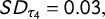
How the different measures compare can be shown through simulations.Footnote ² First off, we investigate their sensitivity to outliers. Figure 1 shows the density distribution of a random sample with $n=10,000$ drawn from a t-distribution with 4 degrees of freedom ( $df$ ). We use the t-distribution since it allows us to simulate a punctuated distribution by controlling $df$ (Fernández-i-Marín et al. Reference Fernández-i-Marín, Hurka, Knill and Steinebach2019). The dashed lines mark the 0.005 and the 0.995 quantiles, therefore, 1% of the values lie outside of the range encompassed by them.

Figure 1 Left: Density distribution of a random sample $n=10,000$ drawn from a t-distribution with $df = 4$ . Right: Normalized measurements of L-kurtosis( $\tau _4$ ), kurtosis (k), and Gini coeefficient (G) for step-wise exclusion of outliers.

The resulting distribution has a high peak with few values deviating strongly from 0. To investigate the effect of outliers on the measures, we removed the 100 largest outliers in a step-wise procedure starting with the largest absolute value and re-estimated the three measures for each outlier removed. Figure 1 shows the resulting measures on the y-axes and the number of outliers removed on the x-axes. The measures were normalized between 0 and 1 to allow for a better comparison. Looking at Figure 1 clearly shows that k is heavily influenced by outliers, with the first three values removed having an immense impact on the measurement. By contrast, $\tau _4$ and G are far more stable, with G being slightly less sensitive. Thus, k is not suited to assess punctuation reliably and we will only concentrate on G and $\tau _4$ in the following.

To compare the measures, we assess if G and $\tau _4$ capture the same concept, as well as their precision. We simulated 10,000 sample distributions with $n = 250$ drawn from a t-distributions with $df = 4$ and estimated G and $\tau _4$ for each sample distribution. Again we use a t-distribution to simulate a punctuated distribution. We choose $n = 250$ as a representation of the typical sample size used in the study of PET.Footnote ³ Since all sample distributions were drawn from the same underlying distribution, variation between them is caused by pure chance. The resulting measures of G and $\tau _4$ are correlated with $p = 0.9$ . Therefore, it can be assumed that both measurements capture the same underlying patterns in the data. Yet, G outperforms $\tau _4$ when it comes to precision.

Figure 2 shows the density distributions for the resulting measures of G and $\tau _4$ with their approximated 95% confidence intervals. The density distribution of G shows a higher peak and less variation than the density distribution of $\tau _4$ . The resulting standard deviations are 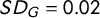$SD_G = 0.02$ and $SD_{\tau _4} = 0.03,$ respectively. When divided by the mean we get coefficients of variation of $CV_G = 0.05$ and $CV_{\tau _4} = 0.15$ . While the difference seems small at first, to reach a similar standard deviation with $\tau _4$ one would have to double the sample size the values are calculated from. For a similar $CV$ it would have to be seven times as large. This finding is not unique to simulated data. We find a similar pattern when applying the two measures to a distribution of U.S. budget outlays. The results are shown in the Supplementary Material.

Figure 2 Density distributions of Gini coefficient (G) and L-kurtois ( $\tau _4$ ) based on 10,000 sample distribution with $n=250$ drawn from t-distribution with $df=4$ .

4 Implications for Type I Errors

The lack of precision has direct implications for the creation of Type I errors, especially for researchers that are interested if change distributions are punctuated or are interested in the comparison between different change distributions (e.g., in the case of varying institutional frictionFootnote ⁴ ). We show this through simulation for the first case and give an empirical example for the second one in the Supplementary Material.

Jones and Baumgartner (Reference Jones and Baumgartner2005) assess punctuation as the deviation of the change pattern from the shape of a normal distribution. This is justified by the assumption that “incremental decision making updated by proportional responses to incoming signals will [ultimately] result in a normal distribution of policy changes” (p. 132). Therefore, the common $H_0$ in PET research is that the change distributions resemble a normal distribution. While G allows us to soften this assumption, since it has an interpretation without referencing the normal distribution, it is helpful to take this baseline to show the proneness for Type I errors of the two measures. In PET research, the hypothesis is often not tested in the classical sense, instead, the literature mostly relies on assessing if $\tau _4$ deviates from the true value of $\tau _4$ for a normal distribution. How this can lead to Type 1 errors can be illustrated through simulation.

First, we calculate an approximation for the true values of G and $\tau _4$ for a standard normal distribution. For this, we simulate 10,000 draws of the size $n = 1,000$ from a standard normal distribution and calculate the measures for each draw. Assuming that the true values converge to the sample mean we obtain $G= 0.414$ and $\tau _4 =0.123$ as the approximately true values. In the literature measures of $\tau _4$ are often taken at face value ignoring their potential imprecision. We create a scenario where a researcher would reject $H_0$ if the obtained value is 0.05 higher than the true value, therefore, 0.173 for $\tau _4$ and 0.464 for G. We then simulate 1,000 draws from a standard normal distribution. For each draw, we calculate the value of G and the value of $\tau _4$ and check if it falls outside the defined rejection criterion. The sample sizes of the drawings are varied from 50 to 500 in one-step increments to account for the fact, that the precision might be worse in smaller samples. Thus, we simulate 1,000 draws of the sample size 50, 1,000 draws of the sample size 51, and so on. Figure 3 shows in percent how often the researcher would wrongly reject $H_0$ for each sample size based on the 1,000 draws and therefore, how often a Type I error is created.

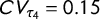
Figure 3 Rejection rate of $H_0$ for G and $\tau _4$ out of 1,000 tries in percent dependent on sample size ranging from 50 to 500. Rejection criterion: Simulated value above 0.05 of true value. Line: LOESS with 95% confidence intervals.

The rejection rate of $\tau _4$ is significantly higher than the rejection rate of G reaching nearly 15% for small sample sizes around 50. Therefore, using G instead of $\tau _4$ could reduce the Type I error rate especially in research scenarios with smaller sample sizes due to its higher precision. One has to keep in mind that the presented scenario still is the most favorable for $\tau _4$ . In cases where researchers are interested in comparing different empirical change distributions, the lack of precision of $\tau _4$ might be even more detrimental. As we show in the Supplementary Material we observe lower precision in empirical distributions that are more punctuated. Therefore, when trying to compare two punctuated distributions the error rate could be much higher.

5 Why Should We Care?

In this letter, we have compared different measures to assess PET. More precisely, we compared the kurtosis and the L-kurtosis with the Gini coefficient and promoted the latter as a better alternative. But why should we care? Why should political research opt for a “new” measure of punctuations after more than two decades (successfully) using the (L-)kurtosis? Most importantly, we argue that it is of great advantage to have a measure that the reader knows and more or less intuitively understands. Most readers have come across the Gini coefficient in the context of income inequality. Moreover, we deem the Lorenz curve to be an intuitive and powerful tool to illustrate the “inequality” of policy change events across time. Knowing that 90% of the changes occurred in only 10% of the time is an easily and uniquely interpretable information. The information that the L-kurtosis is 0.8 does not tell us much without further insights. Yet, it is not only the interpretability that makes the Gini coefficient a superior measure of punctuations. When it comes to assessing change events, political scientists strongly depend on the accuracy of the information provided by experts, research assistants, or computers. These inputs are prone to all kinds of systematic and unsystematic measurement errors. Facing these challenges, we must rely on measures that are least affected by outliers, are the “best possible” estimate of the true value, and are the most precise measure, especially when dealing with rather small sample sizes. The Gini coefficient outperforms the (L-)kurtosis in all these aspects. This gives researchers interested in assessing PET an additional tool to use that can easily be combined with other approaches such as log-log plots, and quantile regression.