One of the central puzzles in the study of American politics is the coexistence of an increasingly polarized Congress with a more centrist electorate (Fiorina and Abrams Reference Fiorina and Abrams2010). Because it has been difficult to find a reliable link between polarization in Congress and the polarization of voter policy preferences, researchers have generally abandoned explanations of congressional polarization that rely on changes in the ideology of the mass public and focus instead on institutional features like primaries, agenda control in the legislature, and redistricting (Fiorina and Abrams Reference Fiorina and Abrams2008; Barber and McCarty Reference Barber and McCarty2013).Footnote 1
This paper brings attention back to the distribution of ideology in the mass public with new data and an alternative theoretical approach. Previous explanations for polarization focus, quite naturally, on variation across the nation as a whole, or on the average or median traits of citizens in each district (e.g., Jacobson Reference Jacobson2004; Clinton Reference Clinton2006; McCarty, Poole and Rosenthal Reference McCarty, Poole and Rosenthal2006; Levendusky Reference Levendusky2009). This work follows from a long literature on representation that builds on Anthony Downs’s (Reference Downs1957) argument that two-candidate competition should lead to platforms that converge on the preferences of the median voter. The great majority of scholarship on this question, however, finds that the median voter is an inadequate predictor of candidate or legislator positions (Miller and Stokes Reference Miller and Stokes1963; Ansolabehere, Snyder and Stewart Reference Ansolabehere, Snyder and Stewart2001; Clinton Reference Clinton2006; Bafumi and Herron Reference Bafumi and Herron2010). Moreover, polarization in Congress (McCarty, Poole and Rosenthal Reference McCarty, Poole and Rosenthal2006; McCarty, Poole and Rosenthal Reference McCarty, Poole and Rosenthal2009) and state legislatures (Shor and McCarty Reference Shor and McCarty2011) has been primarily a reflection of increasing differences in the way Republicans and Democrats represent otherwise similar districts. Consequently, it is unlikely that polarization can be explained purely by changes in the distribution of voter ideology across districts.
We take a different approach. We build upon a literature that focuses on the distribution of voter preferences within districts rather than the distributions of voter medians or means across districts (e.g., Bailey and Brady Reference Bailey and Brady1998; Gerber and Lewis Reference Gerber and Lewis2004; Levendusky and Pope Reference Levendusky and Pope2010; Ensley Reference Ensley2012; Harden and Carsey Reference Harden and Carsey2012; Stephanopoulos Reference Stephanopoulos2012). We show that differences in the roll-call voting behavior of Democratic and Republican legislators are largest in the most ideologically heterogeneous districts. Our main contribution is empirical: this paper is the first to use a large-scale national data set of the votes of about 3000 legislators and the policy views of hundreds of thousands of constituents to test hypotheses about ideological heterogeneity. But first, we motivate these hypotheses with a theoretical model that builds on the work of Calvert (Reference Calvert1985) and Wittman (Reference Wittman1983), who argue that policy-motivated candidates might adopt divergent positions in the face of uncertainty about voter preferences. When candidates are uncertain about the ideological location of the median voter, they shade their platforms toward their or their party’s more extreme ideological preferences. Our extension focuses on mechanisms by which voter heterogeneity produces more uncertainty about the median voter and therefore more polarization.
After presenting the formal model, we turn to an empirical analysis of the roll-call voting behavior of state legislators. Existing research on polarization in the United States focuses primarily on attempting to explain the dramatic growth of polarization in the US Congress (Poole and Rosenthal Reference Poole and Rosenthal1997; McCarty, Poole and Rosenthal Reference McCarty, Poole and Rosenthal2006). The small empirical literature that examines how the distribution of voters’ preferences within districts affects legislators’ roll-call behavior has likewise focused on the US Congress (Bailey and Brady Reference Bailey and Brady1998; Jones Reference Jones2003; Bishin, Dow and Adams Reference Bishin, Dow and Adams2006; Ensley Reference Ensley2012; Harden and Carsey Reference Harden and Carsey2012). The notable exception is Gerber and Lewis (Reference Gerber and Lewis2004) who use data from the California Assembly and Senate.
Congressional polarization has moved in tandem with many potential explanatory variables. Thus, the literature’s exclusive focus on Congress undermines efforts to test competing hypotheses. Moreover, most of the increase in polarization occurred prior to the years for which reliable estimates of voter ideology can be created at the district level. In this paper, we turn away from an analysis of change over time in the US Congress and focus instead on the considerable cross-sectional and more limited longitudinal variation in state legislative polarization.
Our primary focus is on state legislative upper chambers, or state senates. This is a calculated choice that provides a desirable combination of substantial statistical power (several thousand observations of unique state legislators) and good measures of district heterogeneity (hundreds of individual survey respondents within each state Senate district). Congressional districts provide the latter without the former, while state lower chamber (state house or assembly) districts provide even more power, but substantially poorer measures of heterogeneity, based as they are on only a few dozen observations within each district. Nevertheless, we have run our models for both US House and state lower chambers, and have found substantially identical results. These estimates are detailed in the Supplementary Appendix C and D.
Building on the work of McCarty, Poole and Rosenthal (Reference McCarty, Poole and Rosenthal2009), we match upper chamber districts that are as similar as possible with respect to ideology, showing that (1) as in the US Congress, there is considerable divergence in roll-call voting across otherwise identical districts controlled by Democrats and Republicans, and (2) this inter-district divergence is a function of within-district ideological heterogeneity. Given the panel structure of our data, we also have a set of observations of within-district switches in party control. We find that the change in legislator ideal point associated with such a partisan switch is substantially larger in heterogeneous districts.
We conclude with a discussion of the implications of these findings for the polarization literature. Based on our findings, we find it quite plausible that the rise of polarization in the US Congress has been driven in part by increasing within-district heterogeneity associated with the demographic and residential transformations of recent decades. Moreover, our results offer skepticism about redistricting reforms aimed at creating more ideologically heterogeneous districts as a cure for legislative polarization (McCarty, Poole and Rosenthal Reference McCarty, Poole and Rosenthal2009; Masket, Winburn and Wright Reference Masket, Winburn and Wright2012). Finally, the utility of these results for explaining polarization suggests that future research on representation should take seriously the idea that the distribution of preferences within districts may be important for determining the positions of legislators, who must balance competing strategic considerations as well as their own preferences in deciding what policy positions to uphold (Fiorina Reference Fiorina1974). The arrival of very large data sets on public opinion and legislative behavior is now making this type of empirical exercise possible.
POLARIZATION IN THE MASS PUBLIC AND STATE LEGISLATURES
We begin by reviewing some of the stylized facts and research findings that motivate the paper. First, we examine the geographic distribution of voter ideology within states. One of the obstacles to previous research on this topic is that scholars have lacked good measures of the mass public’s ideology at the individual level in each state. Existing research primarily relies on measures of ideological self-placement on relatively small national surveys (Jones Reference Jones2003; Bishin, Dow and Adams Reference Bishin, Dow and Adams2006), economic and demographic characteristics (Bailey and Brady Reference Bailey and Brady1998; Stephanopoulos Reference Stephanopoulos2012), or state-level survey responses (Harden and Carsey Reference Harden and Carsey2012; Kirkland Reference Kirkland2014) to measure preference distributions.Footnote 2 However, Tausanovitch and Warshaw (Reference Tausanovitch and Warshaw2013) demonstrate how to estimate the ideal points of survey respondents from their policy views on several surveys and project them onto a common scale, allowing for vastly larger sample size. They bridge together the ideal points of survey respondents from eight recent large-sample surveys using survey responses on a battery of policy questions. Although these surveys ask different questions, a smaller survey asks questions from all of the other surveys. This “super-survey” facilitates comparisons across all of the other samples. Using a scaling model not unlike factor analysis, they are able to produce a single ideological score for every respondent, which summarizes each respondent’s views on the many policy questions they were asked. See Supplementary Appendix A for more details.
The resulting data set has a measure of the ideological preferences of over 350,000 respondents on a common left-right scale.Footnote 3 The ideal point for a given individual signifies the liberalness or conservativeness of that individual. These data on the ideological preferences of hundreds of thousands of Americans enable us to increase dramatically the size of survey samples for small geographic areas, which makes it possible to characterize not only the mean or median position, but also the nature of the overall distribution of citizens’ ideological preferences within states and legislative districts.
These data enable a new approach to what has become a classic question in American politics: is the mass public responsible for ideological polarization in legislatures? The current literature answers with a tentative “no,” based on time series analysis of the US Congress, where legislative polarization has grown but the ideological distance between Democratic and Republican voters began growing much later and at a slower rate. Addressing the question at the state level requires new data and measures. Using a combination of archival and online data gathering, Shor and McCarty (Reference Shor and McCarty2011) estimated ideal points of members of state legislatures from a large data set of roll-call votes cast between 1993 and 2015. These estimates once again summarize positions on large numbers of roll-call votes using a simple measurement model. However, no comparisons across different states are possible without some method to account for the fact that agendas are vastly different across states. That “bridging” is facilitated by a survey that asks candidates from different states about their policy positions using the same questions (see Shor and McCarty Reference Shor and McCarty2011, 532–3). Individual-level measurements can be then aggregated in a variety of ways to make statements about states as a whole.
Combining the data on ideological distributions of voters and positions of state legislators provides the opportunity to take a first look at the relationship between district heterogeneity and legislative polarization. If legislative polarization is a function of ideological polarization of voters across districts, we would expect to see the familiar bimodal distribution of legislator ideal points mirrored in the distribution of district-level median ideal points of voters. Figure 1 displays kernel densities of both measures across all state upper chambers. There is sharp divergence between the roll-call votes of Democrats and Republicans, but the distribution of median ideology across districts has a single peak. The disjuncture is even more extreme when one examines these distributions separately for each state. Thus Fiorina’s (Reference Fiorina and Abrams2010) puzzle reappears at the district level: there is a large density of moderate districts, but in many states the middle of the ideological distribution is not well represented in state legislatures (Shor Reference Shor2014). The same is true for the US Congress (Rodden Reference Rodden2015).
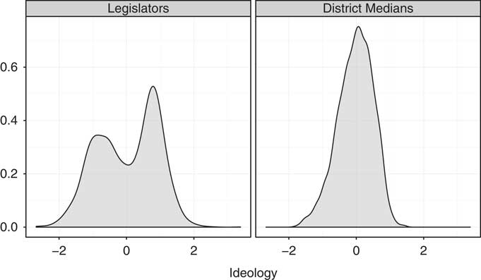
Fig. 1 Distributions of legislator and district median ideal points Note: This plot shows the distribution of legislators’ ideal points and the median citizen’s ideal point in each district. It indicates that the distribution of legislators’ ideal points is much more polarized than the ideal points of the median citizens.
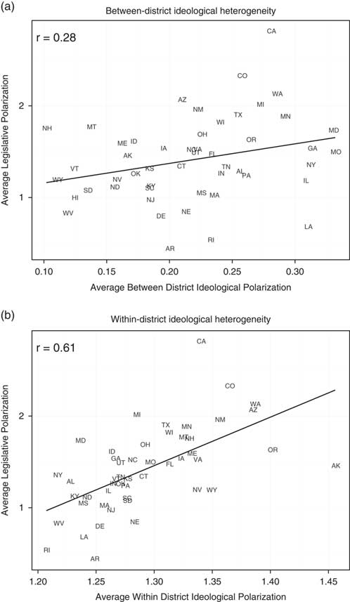
Next, we examine cross-state variation in the polarization of legislatures that we measure as the distance in ideal point estimates between state legislative Democratic and Republican medians (averaged across chambers). A commonly held view is that polarization reflects the way in which voters are allocated across districts. If this were the case, we would expect to see that our measure of legislative polarization correlates strongly with the variation of district medians within each state. In the top panel of Figure 2, we examine this hypothesis by plotting the degree of legislative polarization against across-district ideological heterogeneity in the mass public for each state (measured as the standard deviation of the district-level ideology estimates). Indeed, we find a correspondence between across-district heterogeneity and the polarization of the legislature.

Fig. 2 Legislative polarization and ideological heterogeneity Note: These plots show the correlation between legislative polarization and the between-district (a) and within-district (b) polarization of citizens in each state.
This relationship, however, leaves a large part of the variance unexplained. In the bottom panel of Figure 2 we test a different proposition—that heterogeneity within districts correlates with legislative polarization. The horizontal axis captures the average within-district standard deviation of our ideological scale for district opinion. Again we find a systematic relationship, stronger indeed than that for between-district heterogeneity. Not only is legislative polarization correlated with across-district ideological heterogeneity, but the states with the highest levels of within-district heterogeneity, such as California, Colorado, and Washington, are also clearly those with the highest levels of legislative polarization.
If district heterogeneity impacts polarization, it is important to understand what sorts of districts have this feature. More specifically, what is the relationship between ideology—how conservative or liberal a district is on average—and that district’s heterogeneity? Figure 3 plots our measure of the standard deviation of public ideology for each state senate district on the vertical axis, and our estimate of mean ideology of the district on the horizontal axis. The left side of the inverted u-shape of the lowess plot in Figure 3 shows that the far-left urban enclaves are ideologically relatively homogeneous. The same is true for the conservative exurban and suburban districts on the right side of the plot.Footnote 4
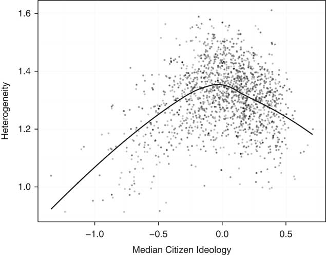
Fig. 3 Average district ideology and within-district polarization Note: This plot shows the relationship between the median citizens’ ideological preferences and the heterogeneity of citizens’ preferences in each state senate district in the country.
The most internally heterogeneous districts are those in the middle of the ideological spectrum. In other words, the districts with the most moderate ideological means—the so-called “purple” districts where the presidential vote share is most evenly split—tend to be places where the electorate is most heterogeneous. These are the districts that switch back and forth between parties in close elections and determine which party controls the state legislature. Reformers often idealize such moderate districts because it is believed that they are most conducive to the political competition that is supposed to produce moderate representation. But as we will show, the fact that such districts are more likely to be heterogeneous mitigates their ability to elect moderate legislators. A takeaway from Figure 3 is that state senate districts come predominately in three flavors: “liberal,” “conservative,” or “moderate but heterogeneous.” Our argument is that none of these are conducive to centrist representation.
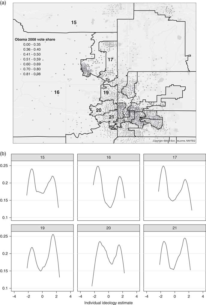
To better understand why moderate districts are so often heterogeneous, it is useful to take a closer look at an example of the distribution of ideology in Colorado, a highly polarized state. The top portion of Figure 4 zooms in on the pivotal “purple” Denver–Boulder suburban corridor, representing the centroids of precincts with dots.Footnote 5 The identification numbers of the districts with the most ideologically moderate means are displayed on the map, and the bottom portion of Figure 4 presents kernel densities capturing the distribution of our ideological scale within each corresponding district.
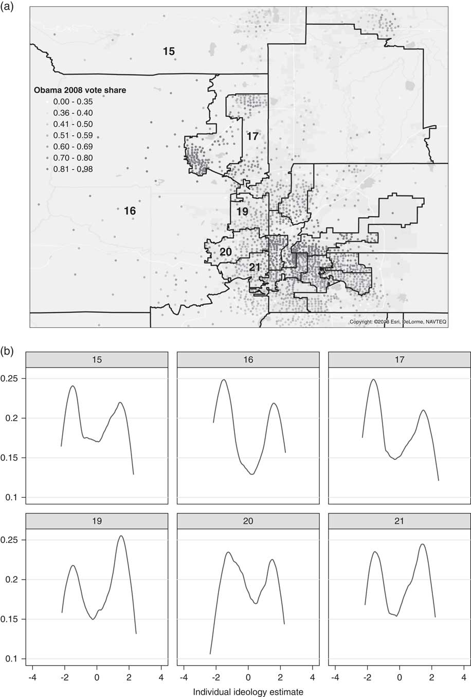
Fig. 4 Within-district distributions of votes and ideology, selected Colorado senate districts Note: (a) Precinct-level 2008 Obama vote share; (b) within-district distribution of ideology, pivotal districts.
The kernel densities show that these “moderate” districts are very heterogeneous internally. Several of these are relatively compact formerly white districts in the suburbs that have experienced large inflows of Hispanics in recent years. These districts contain a mix of Democratic, Republican, and evenly divided precincts. Another type of internally polarized district is exemplified by Districts 15 and 16—sprawling, sparsely populated districts that contain rural conservatives and concentrated pockets of progressives.
Throughout the United States, our estimates of within-district ideology tell a similar story. Districts in the urban core of large cities are homogeneous and liberal. Yet many of their surrounding suburban districts are quite ideologically heterogeneous—a phenomenon that is driven in large part by the growing racial, ethnic, and income heterogeneity of American suburbia (Orfield and Luce Reference Orfield and Luce2013). As for rural districts, some are overwhelmingly white, sparsely populated, and conservative, but in many cases, they also include countervailing concentrations of progressive voters surrounding colleges, resort communities, mines, 19th century manufacturing outposts, or Native American reservations.
These initial findings motivate the remainder of the paper: in the middle of each states’ distribution of districts lies a set of potentially pivotal districts that are ideologically moderate on average, but where voters are often quite heterogeneous and characterized by a lower density of moderates than one might expect. Moreover, this within-district ideological heterogeneity is a good predictor of polarization in state legislatures.
But given the logic of the median voter, why would electoral competition in these pivotal but heterogeneous districts generate such polarized legislative representation? The remainder of the paper develops a simple intuition: relative to a homogeneous district where voters are clustered around the district median, candidates in such heterogeneous districts face weaker incentives for platform convergence due to uncertainty about the ideology of the median voter.
A FORMAL MODEL
In this section, we extend a canonical model of electoral competition to provide some intuition about a possible of linking heterogeneity to polarization. Following Wittman (Reference Wittman1983) and Calvert (Reference Calvert1985), assume that there are two political parties with preferences over a single policy dimension X. Party L prefers that policies be as low as possible and party R wants policy to be as high as possible.Footnote 6 Thus u R (x)=x and u L (x) =−x.
We assume that the parties are uncertain about the distribution of preferences among voters who will turnout in a general election. The parties share common beliefs that the ideal point of the median (and decisive) voter m is given by probability function F. We assume that the median voter has preferences that are single-peaked and symmetric around m.
Prior to the election, parties L and R commit to platforms x
L
and x
R
.Footnote
7
Voter m votes for the party with the closest platform. Therefore, party L wins if and only if
 $$m\leq {{x_{L} {\plus}x_{R} } \over 2}$$
. Therefore, we may write the payoffs for the parties as follows:
$$m\leq {{x_{L} {\plus}x_{R} } \over 2}$$
. Therefore, we may write the payoffs for the parties as follows:
 $$U_{L} (x_{L} ,x_{R} )\,{\equals}\,F\left( {{{x_{L} {\plus}x_{R} } \over 2}} \right)u_{L} (x_{L} ){\plus}\left[ {1\,{\minus}\,F\left( {{{x_{L} {\plus}x_{R} } \over 2}} \right)} \right]u_{L} (x_{R} ),$$
and
 $$U_{R} (x_{L} ,x_{R} )\,{\equals}\,F\left( {{{x_{L} {\plus}x_{R} } \over 2}} \right)u_{R} (x_{L} ){\plus}\left[ {1\,{\minus}\,F\left( {{{x_{L} {\plus}x_{R} } \over 2}} \right)} \right]u_{R} (x_{R} ).$$
The first-order conditions for optimal platforms areFootnote 8
 $${\minus}F\left( {{{x_{L} {\plus}x_{R} } \over 2}} \right){\plus}{1 \over 2}\left[ {F^{'} \left( {{{x_{L} {\plus}x_{R} } \over 2}} \right)} \right](x_{R} \,{\minus}\,x_{L} )\,{\equals}\,0,$$
 $$\left[ {1\,{\minus}\,F\left( {{{x_{L} {\plus}x_{R} } \over 2}} \right)} \right]{\minus}{1 \over 2}\left[ {F^{'} \left( {{{x_{L} {\plus}x_{R} } \over 2}} \right)} \right](x_{R} \,{\minus}\,x_{L} )\,{\equals}\,0.$$
It is straightforward to establish that convergence is not an equilibrium. Suppose x
L
=x
R
=x, then the first-order conditions become F(x)=1−F(x)=0 which obviously cannot hold. Thus, the only candidate equilibrium is one where
 $$x_{L}^{{\asterisk}} \,\lt\,x_{R}^{{\asterisk}} $$
. Thus, when there is uncertainty about the median voter, the candidates diverge in equilibrium. Conversely, if the median voter is known with certainty, then candidates converge as predicted by Downs.
$$x_{L}^{{\asterisk}} \,\lt\,x_{R}^{{\asterisk}} $$
. Thus, when there is uncertainty about the median voter, the candidates diverge in equilibrium. Conversely, if the median voter is known with certainty, then candidates converge as predicted by Downs.
Now, we can establish the direct relationship between uncertainty and polarization by re-writing the first-order conditions as:
 $${{F^{'} \left( {\tilde{x}} \right)} \over {F\left( {\tilde{x}} \right)}}\,{\equals}\,{{F^{'} \left( {\tilde{x}} \right)} \over {1{\minus}F\left( {\tilde{x}} \right)}}\,{\equals}\,{2 \over {x_{R} \,{\minus}\,x_{L} }},$$
where
 $$\tilde{x}\,\equiv\,{{x_{L} {\plus}x_{R} } \over 2}$$
. Equation 5 implies that
$$\tilde{x}\,\equiv\,{{x_{L} {\plus}x_{R} } \over 2}$$
. Equation 5 implies that
 $$1\,{\minus}\,F\left( {\tilde{x}} \right)\,{\equals}\,F\left( {\tilde{x}} \right)$$
which implies that
$$1\,{\minus}\,F\left( {\tilde{x}} \right)\,{\equals}\,F\left( {\tilde{x}} \right)$$
which implies that
 $$\tilde{x}$$
equals the median of F,
$$\tilde{x}$$
equals the median of F,
 $$\bar{m}$$
. Moreover,
$$\bar{m}$$
. Moreover,
 $$x_{R} \,{\minus}\,x_{L} {\equals}{1 \over {F^{'} (\bar{m})}}$$
.
$$x_{R} \,{\minus}\,x_{L} {\equals}{1 \over {F^{'} (\bar{m})}}$$
.
This result is summarized in Proposition 1.
Proposition 1: Let F be a distribution function with median
 $$\bar{m}$$
, then
$$\bar{m}$$
, then
(a) there exists a pure strategy Nash equilibrium such that
 $$x_{L}^{{\asterisk}} \,{\equals}\,\bar{m}\,{\minus}\,{1 \over {2F^{'} (\bar{m})}}$$
and
$$x_{L}^{{\asterisk}} \,{\equals}\,\bar{m}\,{\minus}\,{1 \over {2F^{'} (\bar{m})}}$$
and
 $$x_{R}^{{\asterisk}} \,{\equals}\,\bar{m}{\plus}{1 \over {2F^{'} (\bar{m})}}$$
,
$$x_{R}^{{\asterisk}} \,{\equals}\,\bar{m}{\plus}{1 \over {2F^{'} (\bar{m})}}$$
,
(b) the level of divergence is
 $$x_{R}^{{\asterisk}} \,{\minus}\,x_{L}^{{\asterisk}} \,{\equals}\,{1 \over {F^{'} (\bar{m})}}$$
.
$$x_{R}^{{\asterisk}} \,{\minus}\,x_{L}^{{\asterisk}} \,{\equals}\,{1 \over {F^{'} (\bar{m})}}$$
.
The upshot of the proposition is that the divergence between candidates is proportional to the inverse of the density at the median of the distribution of median voters. When there is a lot of mass around the median of the distribution, electoral competition drives the parties toward convergence. When there is less mass around the median and more in the tails, policy-seeking parties will choose more divergent candidates.
To generate an observable comparative static on the distribution of median voters, we assume somewhat more structure for F. Let F be a member of the symmetric, scalable family of distributions so that
 $$F(m)\,{\equals}\,\bar{F}({{m\,{\minus}\,\bar{m}} \over \sigma })$$
where
$$F(m)\,{\equals}\,\bar{F}({{m\,{\minus}\,\bar{m}} \over \sigma })$$
where
 $$\bar{F}$$
is a symmetric distribution with mean and median of
$$\bar{F}$$
is a symmetric distribution with mean and median of
 $$\bar{m}$$
. Since
$$\bar{m}$$
. Since
 $$\bar{F}$$
is symmetric, the scale parameter σ induces mean- and median-preserving spreads, and is thus directly related to the variance of m. With these additional assumptions, the equilibrium candidate divergence is
$$\bar{F}$$
is symmetric, the scale parameter σ induces mean- and median-preserving spreads, and is thus directly related to the variance of m. With these additional assumptions, the equilibrium candidate divergence is
 $$x_{R}^{{\asterisk}} \,{\minus}\,x_{L}^{{\asterisk}} \,{\equals}\,{\sigma \over {\bar{F}^{'} (0)}}$$
. Thus, divergence is directly proportional to σ and is consequently increasing in the variance of m. This result is stated in the following corollary.
$$x_{R}^{{\asterisk}} \,{\minus}\,x_{L}^{{\asterisk}} \,{\equals}\,{\sigma \over {\bar{F}^{'} (0)}}$$
. Thus, divergence is directly proportional to σ and is consequently increasing in the variance of m. This result is stated in the following corollary.
Corollary 1: If F is symmetric, scalable distribution, in the symmetric Nash equilibrium described in Proposition 1, the equilibrium level of divergence is increasing in the variance of m.
To illustrate the proposition and corollary, consider a couple of examples. First, assume that m is distributed normally with mean 0 and standard deviation s. In this case,
 $$x_{R}^{{\asterisk}} \,{\minus}\,x_{L}^{{\asterisk}} \,{\equals}\,s\sqrt {2\pi } $$
. Therefore, the equilibrium level of divergence is increasing in s. Similarly assume that m is distributed u[−a, a],
$$x_{R}^{{\asterisk}} \,{\minus}\,x_{L}^{{\asterisk}} \,{\equals}\,s\sqrt {2\pi } $$
. Therefore, the equilibrium level of divergence is increasing in s. Similarly assume that m is distributed u[−a, a],
 $$x_{R}^{{\asterisk}} \,{\minus}\,x_{L}^{{\asterisk}} \,{\equals}\,2a$$
. Therefore divergence is increasing in a and hence the variance of m.Footnote
9
$$x_{R}^{{\asterisk}} \,{\minus}\,x_{L}^{{\asterisk}} \,{\equals}\,2a$$
. Therefore divergence is increasing in a and hence the variance of m.Footnote
9
Our results establish that uncertainty about the median voter can contribute to candidate divergence. The next step is to connect uncertainty about the median voter to the underlying preference heterogeneity of the district. To motivate this connection, we assume that beliefs about the distribution of the district median are formed by public pre-election polls of the district.
To keep things simple, assume that parties do not know the distribution of the median voter, have diffuse priors, and rely on a poll with sample size N to generate posterior beliefs about the distribution of m. Let G(x) be the distribution function for voter ideal points. Let μ be the median ideal point and σ 2 be the variance of ideal points—our measure of heterogeneity.
A standard result from sampling theory suggests that the sample median from a poll of N voters is asymptotically distributed normally with mean μ and
 $$s^{2} \,{\equals}\,{1 \over {4(N{\plus}1)(G\prime(\mu ))^{2} }}$$
. Therefore, the variance in the estimate of the median ideal point is a decreasing function of the density of median voter in the district. In turn this implies that the equilibrium level of divergence following a public poll would be
$$s^{2} \,{\equals}\,{1 \over {4(N{\plus}1)(G\prime(\mu ))^{2} }}$$
. Therefore, the variance in the estimate of the median ideal point is a decreasing function of the density of median voter in the district. In turn this implies that the equilibrium level of divergence following a public poll would be
 $$x_{R}^{{\asterisk}} \,{\minus}\,x_{L}^{{\asterisk}} \,{\equals}\,\sqrt {{\pi \over {2(N{\plus}1)G\prime(\mu )^{2} }}} .$$
Thus, given enough data to precisely estimate the density of the median of each district, we could use those estimates as predictors of the level of divergence between the candidates in the district. Unfortunately, while we have a relatively large number of observations per district, precise estimation of the densities G′(μ) remains formidable. But we can, however, use the variance of the distribution in each district as a proxy. For example, if the distribution of voter ideal points is normal, we can directly relate the variance of the estimated median to the variance of the overall median so that
 $$s^{2} {\equals}{{\sigma ^{2} \pi } \over {2(N{\plus}1)}}$$
.Footnote
10
Thus, the equilibrium divergence is
$$s^{2} {\equals}{{\sigma ^{2} \pi } \over {2(N{\plus}1)}}$$
.Footnote
10
Thus, the equilibrium divergence is
 $$x_{R}^{{\asterisk}} \,{\minus}\,x_{L}^{{\asterisk}} \,{\equals}\,{{\sigma \pi } \over {\sqrt {N{\plus}1} }}$$
.
$$x_{R}^{{\asterisk}} \,{\minus}\,x_{L}^{{\asterisk}} \,{\equals}\,{{\sigma \pi } \over {\sqrt {N{\plus}1} }}$$
.
For other distributions, the relationship between G′(μ) and σ 2 is less direct. But there is a large class of parametric distributions for which the density at the median is lower when the variance is larger. Any symmetric distribution such as the t-distribution, uniform, and others symmetric beta family must have this property. Non-symmetric distributions with this property include the log-normal, exponential, and Weibull.
The arguments above show a direct relationship between the variance of the voter ideal points and the level of uncertainty about the location of the median voter for a wide variety of ideal point distributions. Other plausible features of elections also work to strengthen the relationship between heterogeneity and the residual uncertainty following the public poll. One empirically plausible feature is that voters with more extreme ideal points are more likely to turnout on election day. This, of course, has the effect of overweighting the voters with extreme preferences. Consequently, turnout would be generated by a weighted distribution where the weights are highest for extreme voters and lead to more uncertainty about the median following any poll.Footnote 11
Another source of electoral uncertainty are partisan and ideological tides which may lead turnout to be higher or lower in different parts of the ideological spectrum from election to election. The effect of such tides are likely to be magnified in heterogeneous districts.Footnote 12
One might also ask why we rely on measures of heterogeneity rather than directly measure F, the probability distribution of the median voter. The simplest answer is that estimates of F are infeasible. Only recently have district-level data on voter preferences become available. However, even if we could estimate median voters for a set of longitudinal data on each district, this empirical distribution may not closely match the F that is observed by the parties in a specific election. Rational political actors must forecast conditions for each race based on possibly unique features of down-ballot and up-ballot races on the ideological composition of the electorates. A researcher who wishes to estimate F is in the unenviable position of modeling the ex ante expected turnout effects of many different candidates in many different races. Such a modeling exercise, even if feasible, is beyond the scope of this paper.
While the variance of the distribution of preferences is an imperfect predictor of electoral uncertainty, we have shown that the variance of voter ideal points will be associated with electoral uncertainty in a broad class of distributions and assumptions. We recognize that there are many theoretical possibilities that could motivate the link between heterogeneous preferences and legislative polarization. Our intention is to demonstrate one such possibility as a starting point. We would encourage other researchers to examine competing theoretically motivated explanations.
RESEARCH DESIGN
Our formal model suggests the following empirical strategy. We would like to estimate the model:
 $$divergence_{i} \,{\equals}\,\beta {\rm V}(m_{i} ){\plus}\gamma z_{i} {\plus}{\epsilon}_{i} ,$$
where divergence i is the distance between the two-candidates in district i, V(m i ) the variance of the median voter in district i, and z i a set of control variables. The theoretical model suggests that β>0. Unfortunately, we only observe the winning candidates of the elections. Therefore, we follow the approach of McCarty, Poole and Rosenthal (Reference McCarty, Poole and Rosenthal2009), who decompose partisan polarization into roughly two components. The first part, which they term intradistrict divergence is simply the difference between how Democratic and Republican legislators would represent the same district. The remainder, which they term sorting, is the result of the propensity for Democrats to represent liberal districts and for Republicans to represent conservative ones.Footnote 13
To formalize the distinction between divergence and sorting, we can write the difference in party mean ideal points as
 $$E(x\left| R \right.)\,{\minus}\,E(x\left| D \right.)\,{\equals}\,{\int} \left[ {E(x\left| {R,z} \right.){{p(z)} \over {\overline{p} }}\,{\minus}\,E(x\left| {D,z} \right.){{1\,{\minus}\,p(z)} \over {1\,{\minus}\,\overline{p} }}} \right]f(z)dz,$$
where x is an ideal point, R and D are indicators for the party of the representative, and z a vector of district characteristics. We assume that z is distributed according to density function f and that p(z) is the probability that a district with characteristics z elects a Republican. The term
 $$\overline{p} $$
is the average probability of electing a Republican. The average difference between a Republican and Democrat representing a district with characteristics z, E(x|R,z)−E(x|D,z), captures the intradistrict divergence, while variation in p(z) captures the sorting effect.
$$\overline{p} $$
is the average probability of electing a Republican. The average difference between a Republican and Democrat representing a district with characteristics z, E(x|R,z)−E(x|D,z), captures the intradistrict divergence, while variation in p(z) captures the sorting effect.
Estimating the average intradistrict divergence (AIDD) is analogous to estimating the average treatment effect of the non-random assignment of party affiliations to representatives. There is a large literature discussing alternative methods of estimation for this type of analysis. For now we assume that the assignment of party affiliations is based on observables in the vector z. If we assume linearity for the conditional mean functions, that is, E(x|R, z)=β 1+β 2 R+β 3 z, we can estimate the AIDD as the ordinary least squares (OLS) estimate of β 2.
Our claim is that the AIDD is a function of uncertainty over the location of the median voter within districts which we have proxied by the variance of the voter’s ideal points. We use two empirical strategies to examine whether the AIDD is greater in more heterogeneous districts. First, we use OLS-based regression models of the form:
 $$x_{i} \,{\equals}\,\alpha {\plus}\beta _{1} {\rm V}(m_{i} ){\plus}\beta _{2} Party_{i} {\plus}\beta _{3} {\rm V}(m_{i} )xParty_{i} {\plus}\gamma z_{i} {\plus}\delta _{{j[i]}} {\plus}{\epsilon}_{i} ,$$
where x i is the ideological position of the incumbent in district i, Party i an indicator that equals 1 if the incumbent is a Republican and −1 if she is a Democrat, γ a vector of district-level covariates, and δ a random effect for each census division or state. If V(m) has a polarizing effect, β 3>0 as it moves Republicans to the right and Democrats to the left.
One complication is that there may be unobserved factors that lead to across-state variation in polarization (i.e., the distance between parties within each state). For instance, variation in primary type or other institutions could affect polarization. As a result, we subset the data and estimate the model separately for each party. This allows us to use census division and state-level random coefficients to account for anytime invariant, unobserved factors lead to across-state variation in polarization within parties. Thus, our regression models show the relationship between legislators’ ideal points and the amount of district-level heterogeneity within each census division or state, depending on the model. This specification also allows β and other coefficients to vary across parties.
Second, because the functional forms used in our OLS models are somewhat restrictive, we also use matching estimators to check the robustness of our main results (Ho et al. Reference Ho, Imai, King and Stuart2007). Intuitively, these estimators match observations from a control and treatment group that share similar characteristics z and then compute the average difference in roll-call voting behavior for the matched set. We use the bias-corrected estimator developed by Abadie and Imbens (Reference Abadie and Imbens2006) and implemented in R using the Matching package (Sekhon Reference Sekhon2011).Footnote 14 Following McCarty, Poole and Rosenthal (Reference McCarty, Poole and Rosenthal2009) and Shor and McCarty (Reference Shor and McCarty2011), we use matching techniques to estimate the average district divergence for districts with different levels of V(m i ). Specifically, we use matching to estimate the AIDD for districts with “high” and “low” levels of heterogeneity. We define districts with “high” levels of heterogeneity as those that are above the national median, and those with “low” levels of heterogeneity as those that are below the national median.
We estimate the position of the median voter in each district using the approach described in Tausanovitch and Warshaw (Reference Tausanovitch and Warshaw2013). Specifically, we combine our super-survey of 350,000 citizens’ policy preferences with a multilevel regression with post-stratification (MRP) model. Previous work has shown that MRP-based models yield accurate estimates of the public’s preferences at the level of states (Park, Gelman and Bafumi Reference Park, Gelman and Bafumi2004; Lax and Phillips Reference Lax and Phillips2009) as well as congressional and state legislative districts (Warshaw and Rodden Reference Warshaw and Rodden2012; Tausanovitch and Warshaw Reference Tausanovitch and Warshaw2013). As a robustness check, we also run all of our models using presidential vote share in each district as a proxy for the position of the median voter.
Finally, we estimate the variance of the median voter in district i based on the standard deviation of the electorate’s preferences in each district in the large data set of citizens’ ideal points from Tausanovitch and Warshaw (Reference Tausanovitch and Warshaw2013) (Gerber and Lewis Reference Gerber and Lewis2004; Levendusky and Pope Reference Levendusky and Pope2010; Ensley Reference Ensley2012; Harden and Carsey Reference Harden and Carsey2012). In Supplementary Appendix B, we also use an alternative measure of the heterogeneity of preferences in each district that eliminates the possibility that the measure is influenced by sample size. Our results are substantively similar using both definitions of the variance of the median voter in each district.
RESULTS
In this section, we present our main results on the link between the variance of the median voter in each senate district and polarization in legislators’ roll-call behavior.Footnote 15 Before reporting on the multilevel and matching models, we first present some graphical evidence for our argument. Figure 5 shows how legislator ideology changes with district opinion. The three panels represent terciles of district heterogeneity, with the leftmost (or “first”) the least heterogeneous, and the rightmost (“third”) the most heterogeneous. Each point represents a unique legislator serving sometime between 2003 and 2012, with Republicans represented with triangles and Democrats with circles. Both parties are responsive to district opinion, with more conservative districts being represented by more conservative legislators. Nevertheless, a distinct separation between the parties is quite evident. More central to our point, that divergence is largest for the most heterogeneous districts.
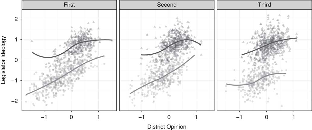
Fig. 5 Scatterplot of legislator ideology and state senate district opinion, by heterogeneity tercile Note: Republicans are represented with triangles and Democrats with circles.
We now turn to our multilevel analyses which are presented in Table 1. The unit of analysis is the unique legislator in Shor and McCarty’s (Reference Shor and McCarty2011) data that served at some point between 2003 and 2012. The two columns show results of a simple multilevel model with varying intercepts for census divisions.Footnote 16 The results indicate that both Democratic and Republican state legislators take substantially more extreme positions in more ideologically heterogeneous districts. AIDD is clearly a function of ideological heterogeneity in the district. Controlling for mean district ideology, the difference between the roll-call voting behavior of Democrats and Republicans within states is largest in districts that are most heterogeneous, and smallest in the most homogeneous districts.Footnote 17 Suggestively, the effect for Republicans appears somewhat higher than that for Democrats (though the difference is not significant at conventional levels). We also find substantively similar results using an alternate measure of ideological heterogeneity which adjusts for sample size at a cost to overall statistical power.Footnote 18
Table 1 Heterogeneity: Upper Chamber Score Models (Multilevel)
Note: *p<0.1; **p<0.05; ***p<0.01.
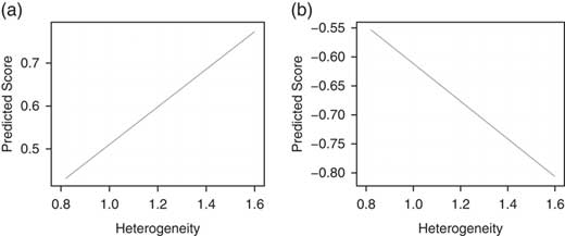
To get a better idea of the size of the effect, consider the first two columns of Table 1. A shift from one-half of a standard deviation below the mean in our heterogeneity measure to one-half of a standard deviation above the mean (from 1.25 to 1.36), while keeping district opinion constant at its mean, is predicted to make Republican legislator ideal points 0.05 units more conservative and Democratic ideal points 0.04 units more liberal. This total 0.09 point shift in AIDD due to an increase of 1 SD of heterogeneity is ~24.2 percent of the mean standard deviation of state legislator ideology by state.Footnote 19 Figure 6 shows these effects more vividly. A district with heterogeneity less than 1.0 can expect to be represented by a moderate, regardless of party. In contrast, districts with heterogeneity of 1.4 or more can expect to be represented by a legislator who is from the extremes of their party.

Fig. 6 Predicted values of Republican (a) and Democratic (b) ideal points as a function of district heterogeneity
Finally, as discussed above, we use matching estimators to check the robustness of our main results. The matching approach tells a similar story to the OLS models. AIDD is substantially greater among matched districts that are more heterogeneous than in those that contain more homogeneous electorates. Table 2 shows that the AIDD in heterogeneous districts is 25 percent greater than in the more homogeneous districts.
Table 2 Matching Estimates of the Average Intradistrict Divergence (AIDD) (Average Treatment Effect) in the Upper Chamber
Clearly, the use of random effects and matching cannot eliminate all concerns about omitted variable bias. To better account for this possibility, we also examine the subset of districts that have been represented by both parties. We do this in two ways. First, we isolate those districts that have elected members from both parties at some point in this decade. Then we measure within-district party divergence as the difference in the average ideal point score of these Democrats and Republicans. Our second approach cuts an even finer distinction. Here, we look at districts that have elected members from both parties within the same year. This would be the case for multi-member districts,Footnote 20 or in the context of a within-year transition from one party to the other due to a special election or appointment because of resignation or death. Figure 7 plots divergence as a function of district opinion heterogeneity in either set of districts. The results are striking; district heterogeneity and legislator partisan divergence are quite strongly related.Footnote 21
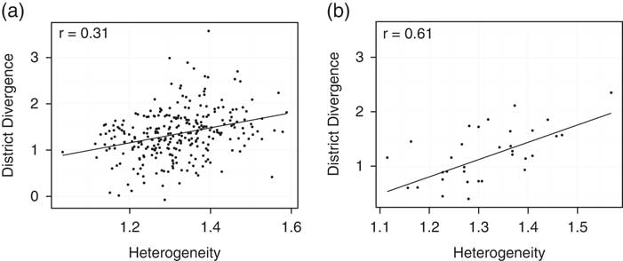
Fig. 7 Scatterplot of district heterogeneity and partisan divergence Note: (a) Within-district: compares the difference between the average ideology of Republicans and Democrats representing a single district anytime from 2003 to 2013. (b) Within-district, within-year: compares the differences between the two parties for districts with multiple representatives for a given year, due either to multi-member districts or mid-year replacement.
One final objection to the conclusions above is that our results may be capturing the effects of primary elections or other nominating contests. We address this in Supplementary Appendix E using analysis that pits our theory against a theory based on primaries. The results are more consistent with a theory based on uncertainty over the median voter.
DISCUSSION AND CONCLUSION
Our key findings can be summarized as follows. Partisan polarization within state legislatures emerges in large part from the fact that Democrats and Republicans represent districts with similar mean characteristics very differently. We have discovered that these differences are especially large in districts that are most internally heterogeneous. Further, we have discovered that these internally diverse districts are especially prevalent in the ideologically “centrist” places that most frequently change partisan hands in the course of electoral competition.
In other words, moderates are often not efficiently clustered in districts where they can dominate. We have identified a class of districts that are moderate on average without containing large densities of moderates. When candidates compete in these internally polarized districts in heterogeneous suburbs and spatially diverse non-metropolitan areas, they face weak incentives to adopt moderate platforms and build up moderate roll-call voting records. Rather, they can cater to primary constituents, donors, activists, or other forces that pull the parties away from the ideological center. We have motivated this intuition with a theoretical model focusing on the candidates’ uncertainty about the ideology of the median voter on election day when the district does not contain a large density of moderates. Aggregating up to the level of states, we have shown that the states with the highest levels of within-district ideological polarization are also those with the highest levels of partisan polarization in the legislature.
Our analysis suggests several avenues for further research. First of all, as larger district-level public opinion samples become available with a longitudinal element, future research might focus more explicitly on the relationship between fluctuations in turnout and the identity of the median voter in different types of districts. Second, it would be useful to develop and test hypotheses about the potential role of primaries and campaign finance in generating divergence of voting behavior in heterogeneous districts.
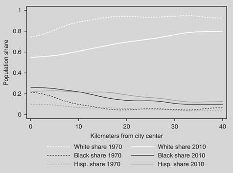
Third, it would be useful to examine whether within-district heterogeneity has risen over time, and whether this can be connected to the rise of polarization in the US House, senate, and state legislatures. We have noted above that many of the ideologically heterogeneous districts are in suburbs that have experienced rapid population change. To visualize this trend, we have collected census tract-level data on race, and measured the distance of the centroid of each tract from the city center in each of the 100 largest metro areas in the United States. Using all of the tracts across 100 cities, Figure 8 displays population shares of African Americans, Latinos, and whites against the distance from the relevant city center, first in 1970 and then in 2010.

Fig. 8 Race, ethnicity, and distance from city center
Figure 8 illuminates a major demographic transformation. If we define suburbia as beginning around 8 km from the city center, we see that inner suburbs were around 85 percent white in 1970, but on average they are barely over 50 percent white today. While falling with distance from the city center, racial heterogeneity extends well out into the middle and more distant suburbs as well. Latinos and especially African Americans were once clustered in city centers, but they are now spread throughout the suburban periphery.
The geography of income has also transformed during the same period. Figure 9 displays box plots of average inflation-adjusted tract-level household income by distance from the city center, first in 1970 and then in 2010. It shows that the heterogeneity of income has grown dramatically throughout metro areas, especially in the suburbs. When legislative districts are drawn in the suburbs, they are likely to encompass an increasingly heterogeneous group of voters with respect not only to race, but also income.
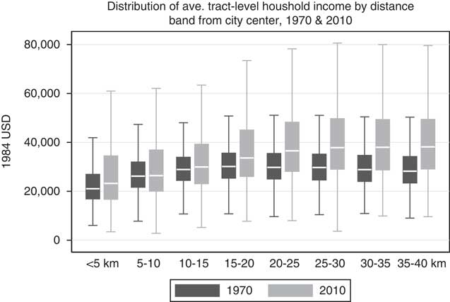
Fig. 9 Income and distance from city center
Finally, our analysis has implications for debates about legislative districting reform. A common claim is that polarization emerges because districts have become too homogeneous, as like-minded Americans have moved into similar communities and politicians have drawn incumbent-protecting gerrymanders. Some reformers advocate the creation of more heterogeneous districts, like California’s sprawling and diverse state senate districts, in order to enhance political competition and encourage the emergence of moderate candidates. This paper turns this conventional wisdom on its head. When control of the legislature hinges on fierce competition within internally polarized winner-take-all districts, candidates, and parties do not necessarily face incentives for policy moderation.