


A number of recent articles in political science have focused on clarifying the meaning of “equation balance” in time series models. While the exact definition differs (c.f., Enns et al., Reference Enns, Kelly, Masaki and Wohlfarth2016; Grant and Lebo, Reference Grant and Lebo2016; Keele et al., Reference Keele, Linn and Webb2016; Enns and Wlezien, Reference Enns and Wlezien2017; Philips, Reference Philips2018), mostly it has centered around the stationarity characteristics of the series, and whether mixed orders of integration can be included in the same model. Scholars have often assessed the performance of two common forms of autoregressive distributed lag (ARDL) models under scenarios with and without equation balance: an ARDL model with the dependent variable appearing in levels—sometimes known simply as a lagged-dependent variable model—and an ARDL model with the dependent variable appearing in first-difference form, often called an error-correction model (ECM).
In this comment, I take an agnostic view of what equation balance means, and simply investigate our ability to gain correct inferences while avoiding incorrect ones, under a variety of data-generating processes for four popular dynamic specifications. While previous articles have assessed the performance of dynamic models under near-integration (De Boef and Granato, Reference De Boef and Granato1997), or how well cointegration tests perform under misspecification (Philips, Reference Philips2018), assessing Type I error in the effects is more rare. I extend analyses that do address Type I error (De Boef and Granato, Reference De Boef and Granato1997; Enns and Wlezien, Reference Enns and Wlezien2017) in two important ways. First, I focus not only on short-run effects, but also long-run effects over a variety of data-generating processes. Second, I examine our ability to get our inferences right when two series are related to one another.
Below, I present a series of Monte Carlo results, discussing the suggested modeling strategy in light of each finding. I conclude by offering suggestions on model specification in dynamic models in general. Such conclusions are important to scholars seeking how to best avoid spurious inferences while still gaining correct ones.
Avoiding incorrect inferences
While avoiding spurious inferences is important in any applied context, the characteristics of time series make them especially pernicious. Therefore, it is crucial for scholars to understand the situations when—in terms of the data-generating process as well as the choice of dynamic specification—Type I error is more or less likely. In this section, I present results from four Monte Carlo analyses. For each, I create two unrelated series, y t and x t—under a variety of different data-generating processes—and regress the two series using four popular model specifications. The first is a purely static model that assumes no dynamics:

Such a model is of course quite common (c.f,. Iversen and Stephens, Reference Iversen and Stephens2008).
The second is an ARDL(1,0) or lagged dependent variable (LDV) model, where the lag of y t also appears on the right-hand side of the equation:

LDV models have been used in a variety of applications, such as the effect of party platform and leadership change on voters’ ideological placement of parties (Fernandez-Vazquez and Somer-Topcu, Reference Fernandez-Vazquez and Somer-Topcu2017).
The third and fourth models are the ARDL(1,1) and the ECM, given respectively as:

and

Since the ECM is simply a re-written version of an ARDL(1,1) model (De Boef and Keele, Reference De Boef and Keele2008), the results below are identical for the ARDL model. Even so, it is still important to show both models, given recent confusion on whether or not they actually differ (Grant and Lebo, Reference Grant and Lebo2016; Enns et al., Reference Enns, Kelly, Masaki and Wohlfarth2016). Moreover, ARDL(1,1) and ECMs are quite popular; examples include how investor heuristics affect sovereign debt markets (Brooks et al., Reference Brooks, Cunha and Mosley2015), or presidential approval and the economy (Ostrom and Smith, Reference Ostrom and Smith1992).
Two quantities are of particular interest. First is the short-run effect of x t on y t, given as β 1 in all equations. In dynamic models, it lends itself to straightforward interpretation since it is analogous to the coefficients in a static model. Second are long-run effects. In dynamic models, these are crucial to understanding the cumulative effect of a change in x t on y t. After De Boef and Keele (Reference De Boef and Keele2008) popularized their utility in political science, long-run effects have appeared in many substantive articles—either analytically (Kelly and Enns, Reference Kelly and Enns2010) or graphically (Brooks et al., Reference Brooks, Cunha and Mosley2015). A statistically significant long-run effect is often used as evidence in support of theoretical expectations. Therefore, it is important to assess the proportion of spurious findings with respect to both short-run and long-run effects. The latter are calculated as follows. They are not present in the static model (Equation 1), since it is assumed there is no persistence in the effect of x t on y t (either through lags of x t or through lags of the dependent variable itself). In Equations 2, 3, and 4, they are, respectively, ${\beta _1\over 1-\alpha }$ , ${( \beta _1 + \beta _2) \over 1-\alpha }$
 , and ${\beta _2\over -\alpha }$
 .
.
Scenario I: Y t ~ I(0), X t ~ I(0)
For the first scenario, both the dependent and independent variables are stationary. However, both contain some amount of persistence in the series, denoted by ϕ y and ϕ x, for the dependent and independent variables, respectively:


I vary the rate of autoregression in each series from 0 to 0.95, by increments of 0.05. ε t, u t ~ N(0, 1) are stochastic terms that are independent from one another.Footnote 1 In total, 2000 simulations were estimated on each combination of ϕ y and ϕ x, across three different time lengths, T = 50, 250, 1000. For each combination of T, ϕ y and ϕ x, I calculated the proportion of times the null hypothesis of no effect was rejected for both the short- and long-run effects.
The results of the all-stationary simulations in Figure 1 indicate that for the ARDL/ECM model, rejection rates of the short-run effects are correctly around 0.05, for both T = 50 and T = 250, no matter the level of autoregression in y t or x t. The same is true for the LDV model, although we are likely to conclude spurious relationships above 10 percent when T = 50 and autoregression in x t and y t nears one. The static model shows the difficulty with modeling time series data without dynamics; Type I error is often above 0.10, rising to over 0.5 when both series are highly autoregressive. Moreover, this gets worse as the series grows longer.Footnote 2 These results are similar to De Boef and Granato (Reference De Boef and Granato1997).
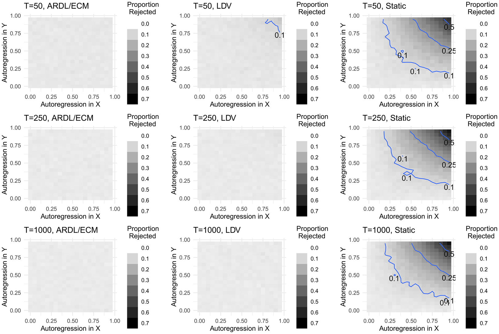
Figure 1. Short-run Type I error, Y t ~ I(0), X t ~ I(0).
Note: Contour lines show boundary of 10, 25, and 50 percent rejection rates.
The results for Type I error for the long-run effects are shown in Figure 2. As is clear from the figure, both the ARDL/ECM and LDV models perform quite well, with the exception of in short series with high autoregression in both y t and x t.
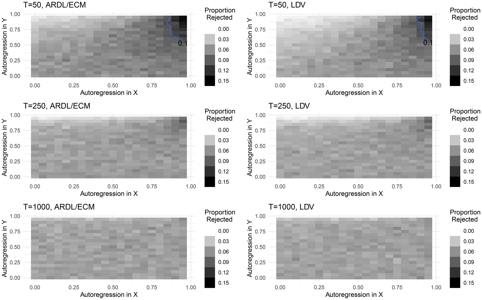
Figure 2. Long-run Type I error, Y t ~ I(0), X t ~ I(0).
Note: Contour lines show boundary of 10 percent rejection rates.
To summarize these findings, when both the dependent and independent variables are stationary yet autoregressive, rejection rates for both the short- and long-run effects are generally around 0.05 for all dynamic models (ARDL/ECM and LDV). The LDV model is not a wise choice if both the independent and dependent variables are highly autoregressive, since short- and long-run rejection rates tend to rise above convention. In addition, one should always avoid the static model if the data-generating processes for x t and y t are plausibly dynamic; in highly autoregressive instances, spurious findings are above 50 percent with the static specification.
Scenario II: Y t ~ I(0), X t ~ I(1)
In the second scenario, the dependent variable remains stationary, yet possibly persistent (given by ϕ y), while the independent variable now contains a unit root (x t = x t−1 + u t). The proportion of times each model commits Type I error across short- and long-run effects is shown in Figure 3. For short-run effects, spurious findings are around convention only for the ARDL/ECM model. The LDV model has slightly higher error rates, but this disappears as the series grows longer. The static model still appears to be the worst performer; when T = 50, ϕ y = 0.5, and x t contains a unit root, spurious inferences occur 40 percent of the time.
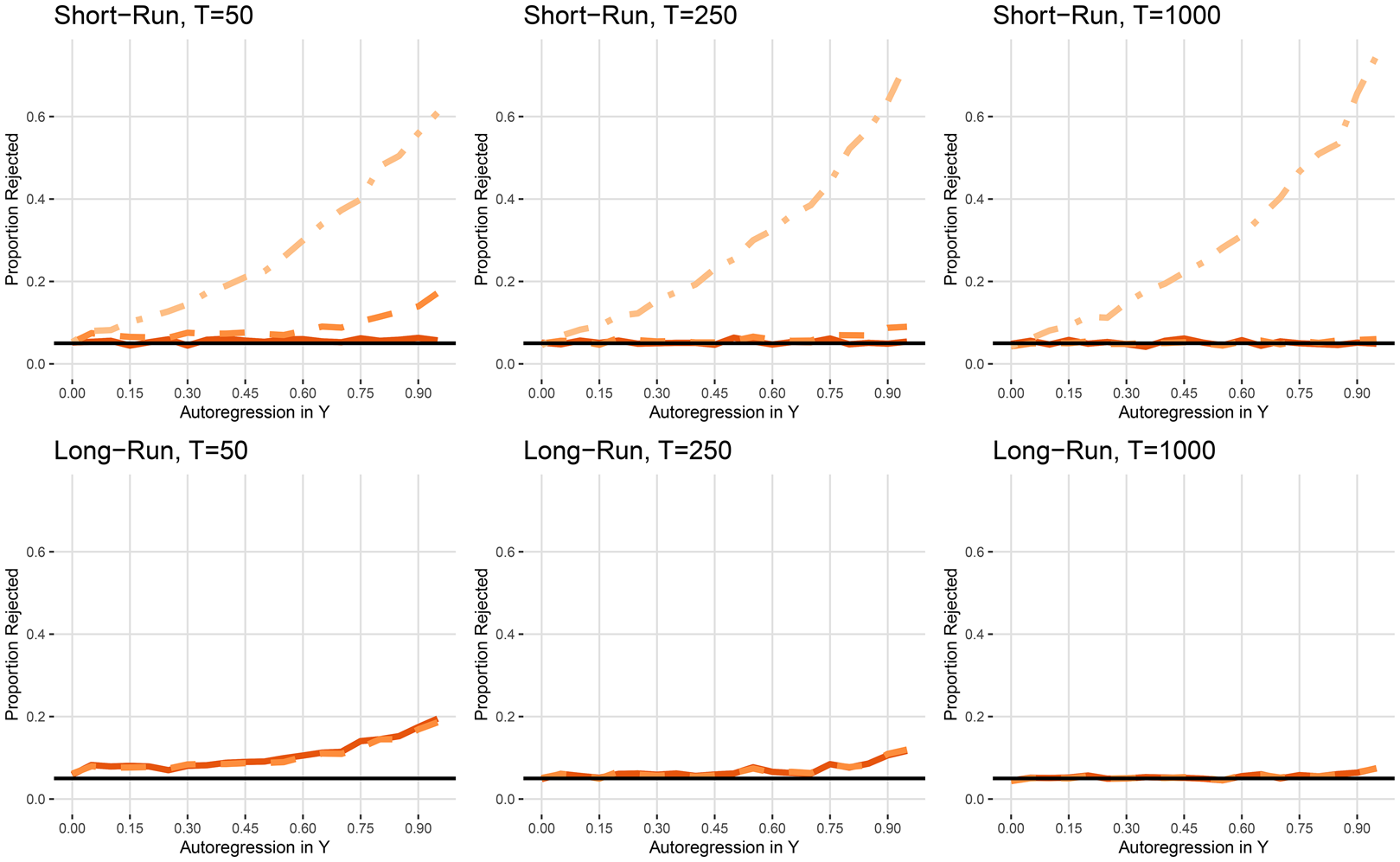
Figure 3. Scenario II: Y t ~ I(0), X t ~ I(1).
Note: Static (dot-dash), LDV (dash), ARDL/ECM (solid). Long-run effects do not exist for static model.
For long-run effects, rejection rates are never at or below 5 percent when T = 50, no matter the level of autoregression, in either the LDV or ARDL/ECM. While Type I error is lower as T increases, it is still clear that as autoregression in the dependent variable increases, high rates of spurious long-run effects result; when T = 50 and ϕ y = 0.85, spurious long-run effects occur about 15 percent of the time using any model.
Given the high rates of spurious long-run effects in this scenario, which model should we choose? Had we diagnosed x t as I(1) and y t as I(0), first differencing x t—thus rendering it stationary—and then including it in the model is advisable.
Scenario III: Y t ~ I(1), X t ~ I(0)
Next, I let the dependent variable contain a unit root, while the independent variable is stationary, but possibly persistent (given by ϕ x). The simulation results are shown in Figure 4. When the dependent variable contains a unit root and the independent variable is stationary, spurious rejection rates for the short-run effect hover around convention, but only for the ARDL/ECM model; the LDV tends to consistently have higher rejection rates, especially when autoregression in x t is high in short series. No matter the length of the series, the static model produces very high Type I error rates.
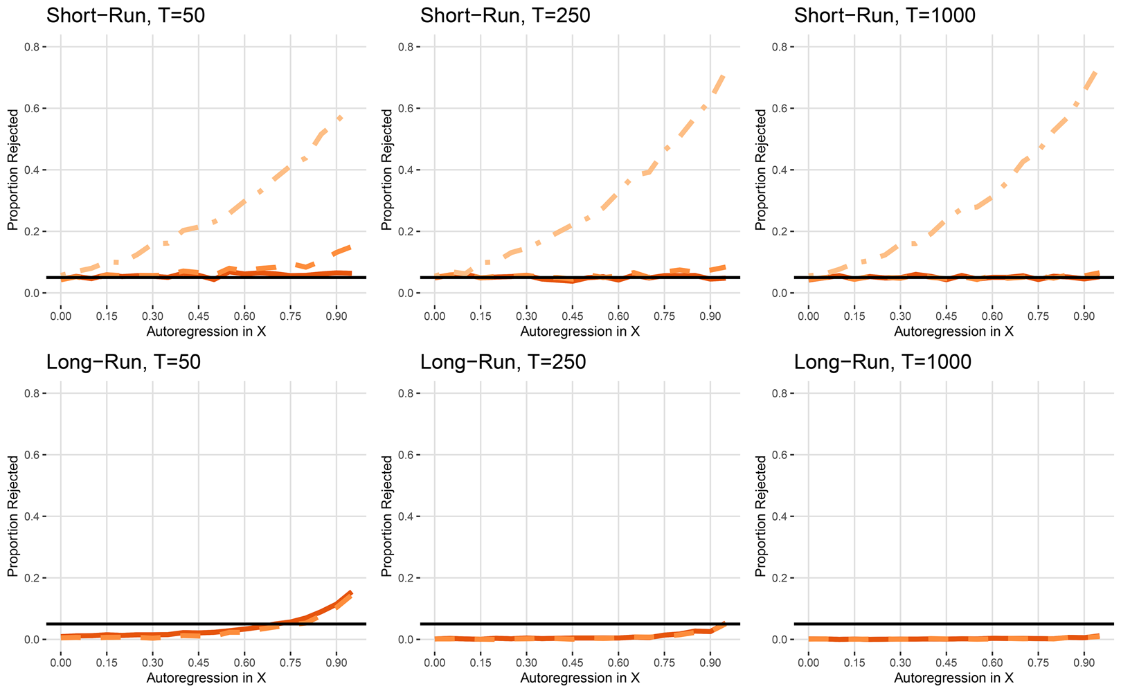
Figure 4. Scenario III: Y t ~ I(1), X t ~ I(0).
Note: Static (dot-dash), LDV (dash), ARDL/ECM (solid). Long-run effects do not exist for static model.
Perhaps surprisingly, rejection rates for the long-run effect are generally lower than 5 percent for both the ARDL/ECM and LDV models; only when autoregression in the independent variable is above 0.7 are rates above convention, and only when T = 50.
Taken with the previous findings, it appears that long-run spurious findings are much more common when the independent variable contains a unit root and the dependent variable is stationary (i.e., Scenario II), than when the dependent variable contains a unit root and the independent variable is stationary.Footnote 3 In this scenario, had we identified that y t was I(1) and x t ~ I(0), we should first difference y t before including it in the model.
Scenario IV: Y t ~ I(1), X t ~ I(1)
A fourth scenario to consider is when y t and x t both contain a unit root. This scenario is well-known in the spurious regression literature in the context of static models (Granger and Newbold, Reference Granger and Newbold1974; Enns et al., Reference Enns, Kelly, Masaki and Wohlfarth2016; Grant and Lebo, Reference Grant and Lebo2016; Philips, Reference Philips2018), although I consider a wider variety of model specifications. As evidenced by Figure 5, the ARDL/ECM model has short-run Type I error rates around convention, no matter the length of the series, while the LDV model has error rates between 0.16 and 0.17, depending on T. The spurious rates for the short-run effects in the static model are astounding, rising to over 85 percent when T = 250, and getting worse as T increases; these echo the original findings by Granger and Newbold (Reference Granger and Newbold1974).
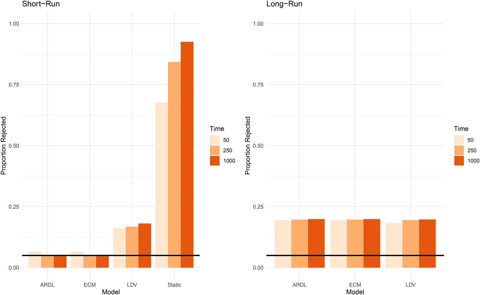
Figure 5. Scenario IV: Y t ~ I(1), X t ~ I(1).
Note: Long-run effects do not exist for static model.
For long-run effects, no model performs close to convention. In fact, both the ARDL/ECM and LDV models have similar Type I error rates of around 0.20. Thus, when both the dependent and independent variables contain a unit root, no model protects against abnormally high rates of spurious regressions for long-run effects. Note too that error rates tend to get worse as the length of the series grows longer (with the exception of the short-run effects for the ARDL/ECM model).
In this scenario, before estimating any model, had we found that both series were I(1) but not cointegrating, we would have known that all four specifications were inappropriate; instead, both series would need to be first-differenced, excluding the possibility of any long-run effect. As is clear from Figure 5, while the ARDL/ECM specifications perform best—especially for short-run inferences—no model can substitute for careful testing and diagnosing the stationarity characteristics of the series.
Getting correct inferences
Scenario V: Y t and X t are stationary and related
While avoiding incorrect inferences is important, so too is getting inferences right. In the next two scenarios, I explore our ability to obtain the correct inferences when two series are related. In this scenario, I create the following stationary DGP:

where x t ~ N(0, 1) and is related to y t with short-run effect β 1 = 2, while α = 0.2, 0.8, and β 2 = 1, − 1 is varied, allowing for different long-run effects, scenarios where the short- and long-run effects are oppositely signed, and varying levels of persistence in y t.
Figure 6 shows the proportion of simulations for which the constructed 95 percent confidence intervals do not overlap with the correct short- and long-run rejection rates.Footnote 4 For the short-run effects (left plots in Figure 6), rejection rates are right around convention for all models. For the long-run effects, when the level of autoregression is low (α = 0.2), the ARDL/ECM rejection rates are around convention, no matter whether the coefficient on x t−1 is positive or negative. In contrast, the LDV model has rates approaching 100 percent when β 2 = −1, but low rates when it is positive. A similar result is found when y t is highly autoregressive. This suggests that, since the LDV is only estimating a single coefficient on x t (and not its lag), if β 2 is substantially different than β 1 (and not zero) then long-run estimates will not be accurate.
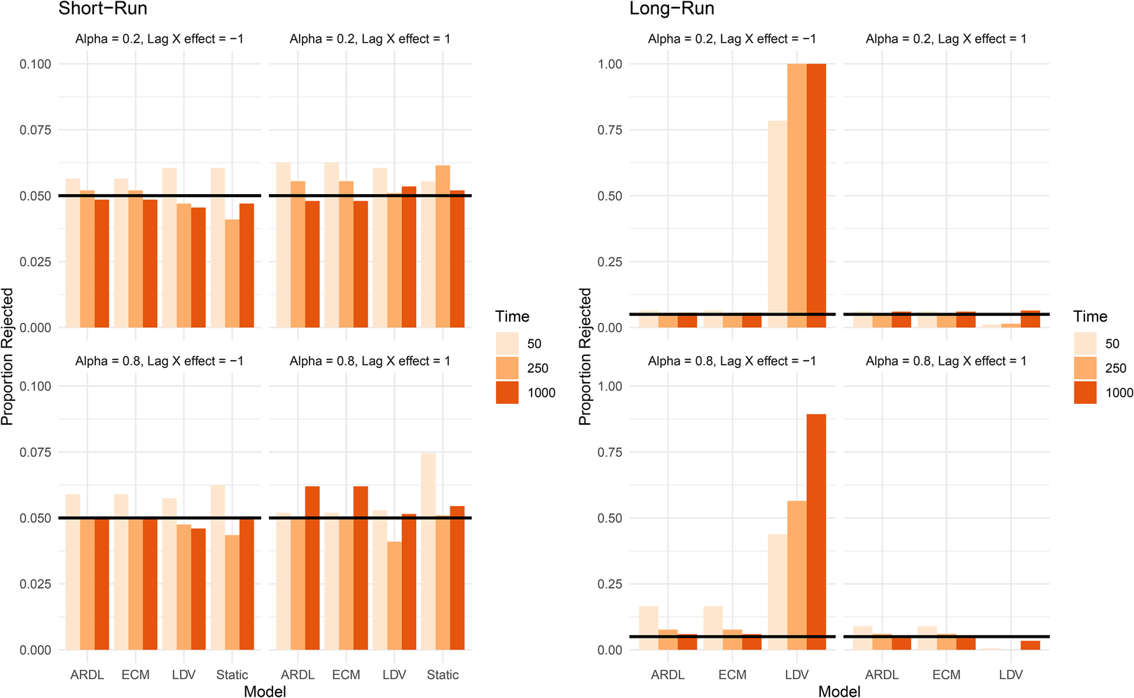
Figure 6. Scenario V: rejection rates of the effects, Y t ~ I(0), X t ~ I(0) and are related.
Note: Long-run effects do not exist for static model.
In the SI, I examine additional quantities of interest. These findings suggest that the most general model—the ARDL/ECM—tends to be the best performer, while the LDV substantially over-estimates the long-run effect, especially when α is small and the coefficients on x t and x t−1 are of opposite sign. Moreover, all model specifications appear to recover short-run effects near convention as T increases.
Scenario VI: Y t and X t are cointegrating
In the last scenario, I examine our ability to obtain correct inferences when both x t and y t are I(1) and cointegrating, specifying the model as follows:

where the short run effect is β 1 = 2, rate of re-equilibration is α = −0.2, − 0.8, and coefficient on x t−1 is β 2 = 1, − 1.
Figure 7 shows the proportion of times the short- and long-run effects are rejected across each model, T, β 2, and α combination. For the short-run effects, both the LDV and static models reject β 1 = 2 nearly 100 percent of the time, while the ARDL/ECM has rejection rates near convention. Additional results in the SI show that the short-run effect is always biased downwards in the LDV, while the static model is either biased upwards or downwards, depending on the value of β 2 and α. Moreover, this does not improve as T increases.
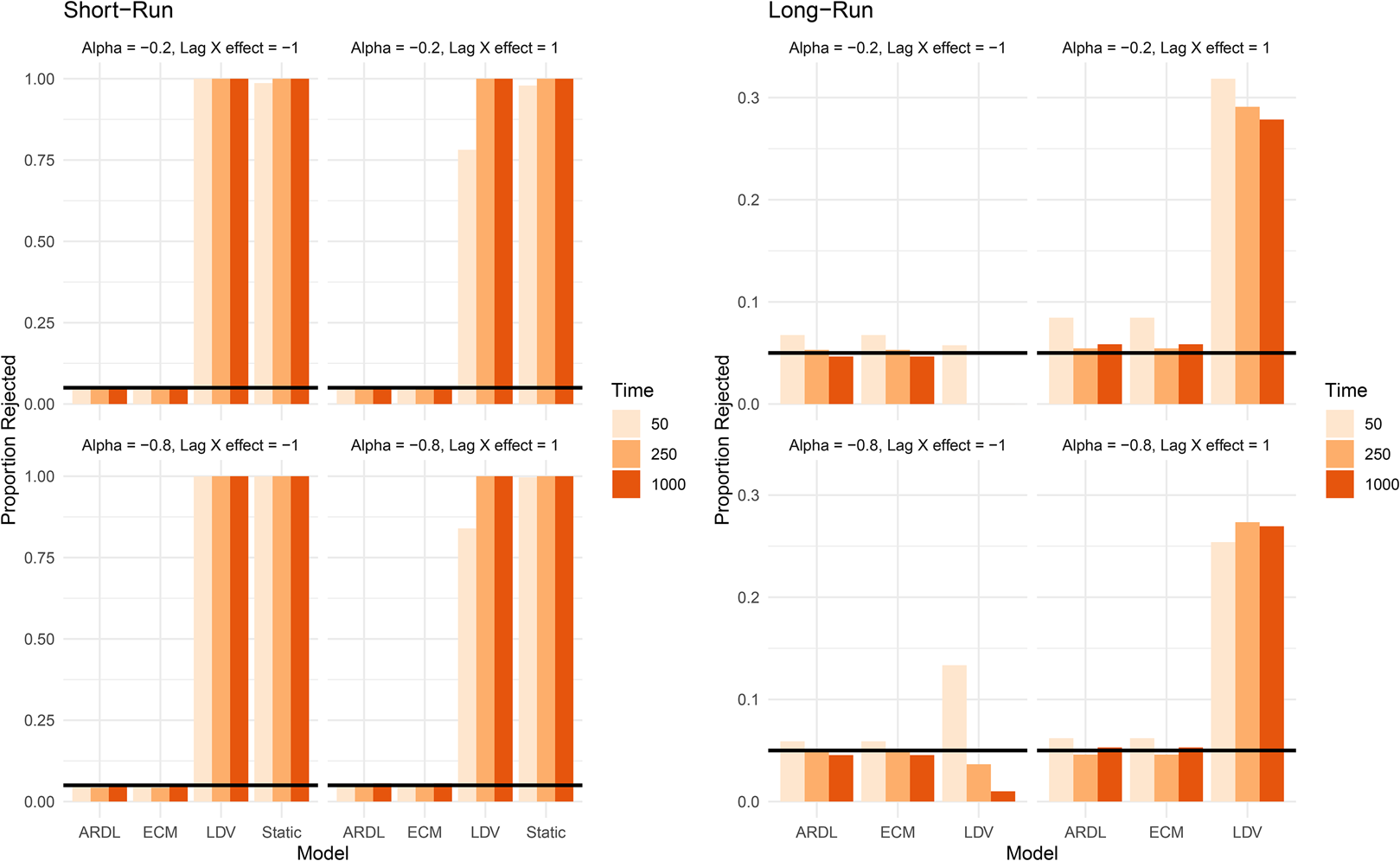
Figure 7. Scenario VI: rejection rates of the effects, Y t ~ I(1), X t ~ I(1) and are cointegrated.
Note: Long-run effects do not exist for static model.
For the long-run effects in Figure 7, rejection rates are near convention as T increases for the ARDL/ECM, although rates are highest in short T if the re-equilibration rate is slow (α = −0.2). In contrast, rejection rates vary drastically in the LDV model. If the coefficient on x t−1 is β 2 = −1, rejection rates of the long-run effect are very low, even near-zero when α = −0.2. In contrast, when β 2 = 1, rates tend to be greater than 25 percent. In other words, the coefficient on x t−1 seems to matter more for the coverage of the long-run effect for the LDV than does the rate of re-equilibration.
Similar to the findings in the previous scenario, results for the cointegrating scenario indicate that the general specification offered by the ARDL/ECM is a wise choice; short-run effects are almost never correctly recovered using the static or LDV models. Moreover, the LDV may not recover the long-run effect, depending on the value of β 2.
What have we learned?
With all of the recent methodological discussions surrounding time series models, what have we learned from these Monte Carlo experiments? First, the static model is never a good strategy if the data-generating process is dynamic. Second, analysts focusing only on short-run effects should not worry about large Type I error rates when using the ARDL/ECM or—in most cases—the LDV. However, finding the correct short-run effect with the LDV almost never occurs when cointegration is present. Third, while correct recovery of long-run effects often occurred with the ARDL/ECM, high Type I error rates were still common with this specification. Fourth, spurious regressions are more common when an I(1) series is regressed on an I(0) one (or vice versa) as the stationary series becomes more autoregressive. This appeared to occur more when the regressor was I(1) (and y t was stationary) than when y t contained a unit root and the regressor was stationary.
Last, the ARDL and ECM models both produced the exact same results in all simulations. While they outperformed the LDV and static model for finding correct inferences due to their flexibility, neither protect the analyst from experiencing Type I error at lower rates than the other. While the ARDL/ECM effectively prevents spurious short-run effects—(see also De Boef and Granato, Reference De Boef and Granato1997; Enns and Wlezien, Reference Enns and Wlezien2017)—spurious inferences at rates higher than convention exist when estimating long-run effects. Given this, one might be tempted to first test for a short-run effect, and then proceed to testing for long-run effects only if the former is significant. Others suggest only calculating a long-run effect if the coefficient on x t−1 is statistically significant (Enns, Moehlecke and Wlezien, this symposium). Such strategies are misguided for several reasons. For one, long-run effects can occur when contemporaneous effects are absent; take dead-start models for instance (De Boef and Keele, Reference De Boef and Keele2008). In addition, power issues and multicollinearity might cause the coefficient on x t−1 to not be significant, even though a long-run effect still exists.Footnote 5 In sum, such strategies will likely reduce Type I error at the cost of our ability to find correct long-run inferences when they exist. I illustrate these points further in the SI.
While readers should take caution in reading too far into these findings—only a limited number of data-generating processes can be presented in a single paper—in the SI, I show a number of additional plots and results, including increasing the error variance in y t, calculating mean square error and power, and plotting the distribution of the effects. These largely comport with the findings above; in general, the ARDL/ECM specification outperforms both the static and LDV model when dynamics are present. However, no model, even the ARDL/ECM, guards against finding evidence of spurious long-run effects in many dynamic contexts. Given this, the following points offer a good starting place for best-practice:
Check stationarity conditions. Checking for stationarity is a crucial first step, as it narrows the possible models that may be used. Unit root testing remains somewhat of an art in short series; conflicting test results, low power, and data characteristics—among them fractional integration, autocorrelation, trends, structural breaks, or periodicity—make determining whether a series is I(0) or I(1) quite difficult. But, as shown above, time series data pose a particularly large threat to inference if the model specification under different stationarity conditions are not considered. One suggestion is to use multiple unit root tests under different assumptions (e.g., a deterministic trend versus no trend); if most tests agree with one another as to whether a series contains a unit root or not, users can be more confident in their stationarity conclusions than by relying on a single test.
Check for cointegration (if applicable). As shown above, equations with I(1) regressors and an I(1) regressand that are not cointegrating are likely to lead to spurious inferences, especially regarding long-run effects. Cointegration testing is relatively straightforward. If evidence for cointegration is not found, the model must be adjusted accordingly in order to avoid spurious inferences.
Lean on the side of caution. Unit root testing is difficult. Even so, spurious regressions occur less frequently where we incorrectly conclude that a series is I(1)—and thus take the first difference—than mistakingly concluding that it is stationary (and do not first difference) (De Boef and Granato, Reference De Boef and Granato1997). Alternatively, practitioners might see if their findings are robust to alternative conclusions about the characteristics of the series.
Ensure the model is well-specified. General-to-specific modeling approaches such as starting with an ARDL/ECM can be used, alongside information criteria and/or statistical significance in order to parse down the model (De Boef and Keele, Reference De Boef and Keele2008; Pickup, Reference Pickup2014). Including a trend and incorporating augmenting lags and/or lagged first differences to correct for residual autocorrelation offers an additional cautious approach (Philips, Reference Philips2018). Models could also be compared using out-of-sample forecasting. Once a suitable model is found, checking for parameter stability and ensuring white-noise residuals are crucial to ensure reliable inferences can be drawn. Practitioners should think carefully not only about their theoretical expectations, but also these expectations in light of whether they conclude that the series are stationary or integrated. For instance, since a unit-root process dominates an I(1) series, it seems hard to advance a theory of how a stationary series could affect it in anything other than the short-run.
Conclusion
Given recent methodological discussions surrounding this model, it should now be obvious that the ECM is not suitable for all applications. Failing to correctly diagnose the correct time series properties and adjusting the model accordingly can be harmful for inference. When series are related and dynamic, estimating a general model like the ARDL/ECM seems a wise choice, since the LDV and static models are simply restricted versions of the former. However, although the ARDL/ECM avoid Type I error better than the LDV or static models, spurious inferences are still common for long-run effects. To guard against these issues, analysts must carefully test and diagnose the characteristics of each of their series in order to gain correct inferences while avoiding spurious ones. As I have shown, the choice of model specification is crucial, since it may lead political scientists to find evidence of relationships when they do not exist, or—conversely—lead them to fail to find evidence when they do.
Supplementary material
The supplementary material for this article can be found at https://doi.org/10.1017/psrm.2021.31.
Acknowledgments
I thank two anonymous reviewers and the current and previous editor for helpful comments and suggestions. Many previous conversations with Lorena Barberia, Soren Jordan, Clayton Webb, Paul Kellstedt, Suzanna Linn, Mark Pickup, and Guy Whitten have also proved invaluable. Nevertheless, all errors are my own.


 Open access