The fixed effects regression model is commonly used to reduce selection bias in the estimation of causal effects in observational data by eliminating large portions of variation thought to contain confounding factors. For example, when units in a panel data set are thought to differ systematically from one another in unobserved ways that affect the outcome of interest, unit fixed effects are often used since they eliminate all between-unit variation, producing an estimate of a variable’s average effect within units over time (Allison Reference Allison2009; Wooldridge Reference Wooldridge2010). Despite this feature, social scientists often fail to acknowledge the large reduction in variation imposed by fixed effects. This article discusses two important implications of this omission: imprecision in descriptions of the variation being studied and the use of implausible counterfactuals—discussions of the effect of shifts in an independent variable that are rarely or never observed within units—to characterize substantive effects.
By using fixed effects, researchers make not only a methodological choice but a substantive one (Bell and Jones Reference Bell and Jones2015), narrowing the analysis to particular dimensions of the data, such as within-country (i.e., over time) variation. By prioritizing within-unit variation, researchers forgo the opportunity to explain between-unit variation since it is rarely the case that between-unit variation will yield plausible estimates of a causal effect. When using fixed effects, researchers should emphasize the variation that is being used in descriptions of their results. Identifying which units actually vary over time (in the case of unit fixed effects) is also crucial for gauging the generalizability of results, since units without variation provide no information during one-way unit-fixed effects estimation (Plümper and Troeger Reference Plümper and Troeger2007).Footnote 1
In addition, because the within-unit variation is always smaller (or at least, no larger) than the overall variation in the independent variable, researchers should use within-unit variation to motivate counterfactuals when discussing the substantive impact of a treatment. For example, if only within-country variation in some treatment X is used to estimate a causal effect, researchers should avoid discussing the effect of changes in X that are larger than any changes observed within units in the data. Besides being unlikely to ever occur in the real world, such “extreme counterfactuals,” which extrapolate to regions of sparse (or nonexistent) data rest on strong modeling assumptions, and can produce severely biased estimates of a variable’s effect if those assumptions fail (King and Zeng Reference King and Zeng2006).
In what follows, we replicate several recently published articles in top social science journals that used fixed effects. Our intention is not to cast doubt on the general conclusions of these studies, but merely to demonstrate how adequately acknowledging the variance reduction imposed by fixed effects—and formulating plausible counterfactuals after estimation that account for this reduction—can improve descriptions of the substantive significance of results.Footnote 2 We conclude with a checklist to help researchers improve discussion of fixed effects results.
VARIANCE REDUCTION WITH FIXED EFFECTS
Consider the standard fixed effects dummy variable model:
 $$Y_{{it}} \,{\equals}\,\alpha _{i} {\plus}\beta X_{{it}} {\plus}{\varepsilon}_{{it}} ,$$
in which an outcome Y and an independent variable (treatment) X are observed for each unit i (e.g., countries) over multiple time periods t (e.g., years), and a mutually exclusive intercept shift, α, is estimated for each unit i to capture the distinctive, time-invariant features of each unit. This results in an estimate of β that is purged of the influence of between-unit time-invariant confounders.Footnote 3
While the overall variation in the independent variable may be large, the within-unit variation used to estimate β may be much smaller. The same is true when dummies for time are included (i.e., year dummies), in which case β is estimated using only within-year variation in the treatment. When multi-way fixed effects are employed (e.g., country and year dummies, as in a generalized difference-in-differences estimator),Footnote 4 the variance reduction is even more severe.
PUBLISHED EXAMPLES
To evaluate how often researchers acknowledge the variance reduction imposed by fixed effects when interpreting results, we conducted a literature review of empirical studies published in the American Political Science Review or the American Journal of Political Science, which used linear fixed effects estimators between 2008 and 2015.Footnote 5 Of the 54 studies we identified fitting these parameters, roughly 69 percent of studies explicitly described the variation being used during estimation (e.g., “… we include a full set of industry-year fixed effects … so that comparisons are within industry-year cells” (Earle and Gehlbach Reference Earle and Gehlbach2015, 713)). Only one study, Nepal, Bohara and Gawande (Reference Nepal, Bohara and Gawande2011), explicitly quantified the size of typical shifts in levels of the treatment within units, allowing readers to judge the plausibility of the counterfactuals being discussed.Footnote 6
Attention to this variance reduction has the potential to greatly influence how researchers characterize the substantive significance of results (i.e., whether a treatment imposes an effect large enough to induce a politically meaningful change in the outcome). For example, Figure 1 shows the distribution of the treatment in Snyder and Strömberg (Reference Snyder and Strömberg2010) before and after fixed effects are applied.Footnote 7 This study estimates the effects of media market congruence (the alignment between print media markets and US congressional incumbents, a continuous variable takes values between 0 and 1), on both the public and political elites. As the left panel of the plot shows, the distribution of congruence is fairly uniform across congressional incumbents and years in the pooled sample. However, once year and incumbent fixed effects are applied, the amount of variation is drastically reduced (the standard deviation of the variable drops from 0.286 to 0.068, a reduction of 76 percent). The reason is that much of the variation in these data is between incumbents, all of which is discarded by the inclusion of incumbent dummies in several models in this study. The right panel of the figure shows the distribution of within-incumbent ranges of the treatment. As the histogram shows, the mean range observed within incumbents is roughly 0.05, and is about 0.36 at the 95th percentile of the distribution of ranges. Roughly 44 percent of the time, the treatment does not vary at all within unit. Noting this fact would help to inform the generalizability of the result.
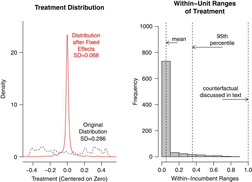
Fig. 1 The left panel displays the distribution of the treatment, media congruence, from Snyder and Strömberg (2010) before and after the incumbent and year fixed effects used in that study are applied Note: Both distributions were centered on 0 before plotting to ease comparisons of their spread. The right panel shows the within-incumbent ranges of the treatment. While the right panel does not perfectly capture the relevant variation since it does not account for two-way fixed effects, we include it here to help motivate within-unit counterfactuals.
While Snyder and Strömberg (Reference Snyder and Strömberg2010) acknowledge the use of a within-unit estimator,Footnote 8 the authors go on to consider a 0-to-1 shift in the treatment when discussing its impact on the probability that an individual recalls the name of their member of Congress. The paper states that, “… a change from the lowest to the highest values of congruence is associated with a 28 percent increase in the probability of correctly recalling a candidate’s name. This is about as large as the effect of changing a respondent’s education from grade school to some college” (Snyder and Strömberg Reference Snyder and Strömberg2010, 372). A 0-to-1 shift is beyond the observed range even in the original data (i.e., before the fixed effects adjustment). When a more realistic counterfactual is used—the standard deviation of the treatment after residualizing with respect to the incumbent and year dummies the authors employ—a more modest effect of a 1.9 percentage point increase in the probability of recalling a representative’s name is recovered. A shift the size of the 95th percentile of within-incumbent ranges produces a 9.9 percentage point effect. Apart from rare cases in which very large shifts in congruence occur within units over time, the results suggest that the treatment exerts only a small effect on representative name recall.
In another example, Ichino and Nathan (Reference Ichino and Nathan2013) discuss the effect of changing the level of an ethnic group surrounding a polling station, stating that, “… a one standard deviation increase in the spatially weighted population share of Akans beyond a polling station (about 0.21) results in a predicted 6.9 percentage point greater NPP presidential vote share” (Ichino and Nathan Reference Ichino and Nathan2013, 351–2). This counterfactual is based on the standard deviation of the overall distribution of the independent variable. However, the fixed effects estimator employed in this analysis only uses the within-parliamentary constituency distribution, and a 1-SD shift in this revised distribution produces a 2.6 percentage point effect, a decrease of 63 percent compared with the reported effect.
Table 1 displays results from replications of five published studies.Footnote
9
In each case, we generated the revised version of the independent variable after residualizing with respect to the included fixed effects (we label this residualized variable
 $$\tilde{x}$$
), in order to assess the consequences of variance reduction. As the results show, considering a 1 SD shift in
$$\tilde{x}$$
, as opposed to a 1-SD shift in the original distribution, reduces estimated treatment effects by as much as 76 percent (column 4). Column 5 compares the counterfactual shifts in X discussed in each article to
$$\tilde{x}$$
), in order to assess the consequences of variance reduction. As the results show, considering a 1 SD shift in
$$\tilde{x}$$
, as opposed to a 1-SD shift in the original distribution, reduces estimated treatment effects by as much as 76 percent (column 4). Column 5 compares the counterfactual shifts in X discussed in each article to
 $$\widehat{{{\rm SD}}}(\tilde{x})$$
. In the case of Berrebi and Klor (Reference Berrebi and Klor2008), the discussed counterfactual is quite plausible (i.e., the ratio is close to 1), while the counterfactuals discussed in Gasper and Reeves (Reference Gasper and Reeves2011) and Ichino and Nathan (Reference Ichino and Nathan2013) are close to three times the size of the revised standard deviation. The changes in X discussed in Scheve and Stasavage (Reference Scheve and Stasavage2012) and Snyder and Strömberg (Reference Snyder and Strömberg2010)—both shifts from the minimum to the maximum of the independent variable’s range—are roughly 9 and 15 times the size of a typical shift in the revised distribution in X, respectively, indicating that changes this large are rarely observed in the data.Footnote
10
$$\widehat{{{\rm SD}}}(\tilde{x})$$
. In the case of Berrebi and Klor (Reference Berrebi and Klor2008), the discussed counterfactual is quite plausible (i.e., the ratio is close to 1), while the counterfactuals discussed in Gasper and Reeves (Reference Gasper and Reeves2011) and Ichino and Nathan (Reference Ichino and Nathan2013) are close to three times the size of the revised standard deviation. The changes in X discussed in Scheve and Stasavage (Reference Scheve and Stasavage2012) and Snyder and Strömberg (Reference Snyder and Strömberg2010)—both shifts from the minimum to the maximum of the independent variable’s range—are roughly 9 and 15 times the size of a typical shift in the revised distribution in X, respectively, indicating that changes this large are rarely observed in the data.Footnote
10
Table 1 Replication Results from Recent Studies Using Fixed Effects
Note: Column 1 displays the estimated unstandardized regression coefficient of interest in each study. Columns 2 and 3 display the standard deviations of the key independent variable before and after residualizing with respect to fixed effects, respectively. Column 4 displays the percent difference between these two SDs. Column 5 displays the ratio of the counterfactual change in the treatment discussed in the article versus our preferred counterfactual, the revised standard deviation of X. See Appendix for details on the referenced published counterfactuals.
Since most political science studies using fixed effects seek to characterize on-average effects rather than effects within any particular unit, we consider the within-unit standard deviation a sensible counterfactual to consider since it represents the average amount the independent variable deviates from the mean after fixed effects are employed. Still, some might wish to convey treatment effects in the common scenario of a one-unit shift. This may be especially useful if the treatment being studied is dichotomous or a count variable that takes only integer values, in which case unit shifts arguably make more substantive sense to consider (this is the case with Berrebi and Klor (Reference Berrebi and Klor2008) and Gasper and Reeves (Reference Gasper and Reeves2011), for example). Here too, variance reduction should be noted, since in some cases even a one-unit shift can represent a change that is several times the size of a typical shift within units. Researchers are of course free to discuss such counterfactuals, but we recommend discussing the magnitude of the hypothetical change in X relative to the variation being used during estimation (i.e., the ratio displayed in column 5) so readers have a sense of whether the hypothetical change in X is rare.
CONCLUSION
Because it reduces concerns that omitted variables drive any associations between dependent and independent variables, many researchers use linear fixed effects regression. This estimator reduces the variance in the independent variable and narrows the scope of a study to a subset of the overall variation in the data set. While some researchers readily acknowledge these features, many studies can benefit from more specificity in the description of the variation being studied and the consideration of counterfactuals that are plausible given the variation being used for estimation (e.g., a typical within-unit shift in X).
CHECKLIST FOR INTERPRETING FIXED EFFECTS RESULTS
When researchers employ linear fixed effects models, we recommendFootnote 11 the following method for evaluating results after estimation:
1. Isolate relevant variation in the treatment: Residualize the key independent variable with respect to the fixed effects being employed (Lovell Reference Lovell1963). That is, regress the treatment on the dummy variables which comprise the fixed effects and store the resulting vector of residuals. This vector represents the variation in X that is used to estimate the coefficient of interest in the fixed effects model.Footnote 12
2. Identify a plausible counterfactual shift in X given the data: Generate a histogram (as in Figure 1) of the within-unit ranges of the treatment to get a sense of the relevant shifts in X that occur in the data. Compute the standard deviation of the transformed (residualized) independent variable, which can be thought of as a typical shift in the portion of the independent variable that is being used during the fixed effects estimation. Multiply the estimated coefficient of interest by the revised standard deviation of the independent variable to assess substantive importance. Note for readers what share of observations do not exhibit any variation within units to help characterize the generalizability of the result. Alternatively, if describing the effect of a one-unit shift, or any other quantity, note the ratio of this shift in X to the within-unit standard deviation, as well as its location on the recommended histogram, to gauge how typically a shift of this size occurs within units.
3. Clarify the variation being studied: In describing the scope of the research and in discussing results after fixed effects estimation, researchers should clarify which variation is being used to estimate the coefficient of interest. For example, if only within-unit variation is being used, then phrases like “as X changes within countries over time, Y changes …” should be used when describing treatment effects.
4. Consider the outcome scale: Consider characterizing this new effect in terms of both the outcome’s units and in terms of standard deviations of the original and transformed outcome (i.e., the outcome residualized with respect to fixed effects). The substance of particular studies should be used to guide which outcome scale is most relevant.