


Introduction
Mixed-methods research designs have gained popularity (Collier and Elman, Reference Collier, Elman, Box-Steffensmeier, Brady and Collier2008; Niedzwiecki and Nunnally, Reference Niedzwiecki and Nunnally2017), and scholars seeking guidance for case selection can draw on a growing literature (e.g., Lieberman Reference Lieberman2005; Gerring Reference Gerring, Box-Steffensmeier, Brady and Collier2008; Seawright and Gerring Reference Seawright and Gerring2008; Seawright Reference Seawright2016a). Case selection in mixed-methods designs is often regression-based, and a recent special issue on case selection emphasized that quantitative tools “should be enlisted, wherever possible, as the procedure is transparent and replicable, it limits opportunities for cherry-picking, and it enhances claims for representativeness” (Elman, Gerring, and Mahoney Reference Elman, Gerring and Mahoney2016: 383).
We show how the quantitative-to-qualitative model of multimethod research can be enhanced with spatial econometric techniques for case selection. While geo-spatial analysis has also received increased attention in the social sciences (e.g., Whitten Reference Whitten2016), existing work neglects the application of such tools for case selection. Although there are many ways to combine methods, for our purposes we assume that the cases chosen for qualitative study are “nested” (Lieberman Reference Lieberman2005) or “embedded” (Hollstein, Reference Hollstein, Dominguez and Hollstein2014) within a larger sample being studied quantitatively. That is, our approach builds on the tradition of “integrated” research designs (Seawright, Reference Seawright2016a; Goertz, Reference Goertz2017). The added value of spatial techniques, as we show throughout the paper, is that they explicitly account for the interdependence of units; case selection techniques that exploit this information create new opportunities for hypothesis generation and theory development.
We begin by briefly reviewing the literature on spatial or geographic approaches to the social sciences, and outline how thinking about the sources of spatial patterns can provide leverage for developing theory. As many of the conceptual, theoretical and methodological components of spatial analysis translate well to other fields of inquiry with dependent (especially networked) data, our guidelines can be adapted for research in a wide range of fields. Further, as one of the paper's main aims is to render the discussion of relevant spatial techniques accessible to readers who have limited familiarity with spatial analysis, we adopt a non-technical style and focus on the motivations for using these techniques.
The core of our paper outlines two main options for mixed-methods research with spatially dependent data (summarized in Table 1). The techniques apply spatial clustering statistics—local indicators of spatial association or LISA (Anselin, Reference Anselin1995)—to (1) the outcome of interest to better understand how a phenomenon is distributed in space, and (2) residuals from a baseline model to examine the geographic structure in the error term. The former technique allows scholars to identify cases based on the varying spatial association of an outcome of interest, including identifying where the outcome of interest maps (or fails to map) onto existing administrative boundaries, and select promising sites for qualitative research geared towards examining the causal process underlying clustering of the outcome. The latter technique allows scholars to select cases based on the varying spatial association of residuals, identifying geographic regions where the model performs well and regions where the model performs poorly. Identifying these regions can help analysts understand where an unknown factor might be exerting a common effect across a set of units, leveraging geography for qualitative research geared towards identifying omitted variables (e.g., Seawright Reference Seawright2016b).
TABLE 1. Overview of Options
Although the options we propose draw on geo-spatial tools, our approach does not require a fully specified theory of spatial interaction based on geographic contiguity or proximity (e.g., Goodchild and Janelle Reference Goodchild and Janelle2010). Rather, we argue that the use of geo-spatial tools to integrate quantitative and qualitative analysis can guide scholars on how and where to look for answers to existing questions and to ask new questions. King (Reference King1996: 160–161) argues that the goal of political geography “should be to try as hard as possible to make context not count” and that geography is particularly powerful “in revealing features of data and the political world that we would not otherwise have considered.” Context, in other words, is a placeholder for causal mechanisms or predictors yet to be identified, and our tools direct attention to promising places in which to examine relevant properties that would otherwise be subsumed generically under “context”. In this way, our approach here speaks to the larger issue of using nominal or “dummy” variables to capture local or regional factors that scholars expect to exert an influence—albeit an influence that may not be clearly identified, much less fully theorized (Ahram, Reference Ahram2011)—and we offer techniques to identify what is meaningful about a particular context.
At the outset, we emphasize that the notion of what constitutes a “case” may be different in mixed-method studies following our proposed strategies than in traditional regression-based designs. Existing approaches to case selection focus on identifying single units for in-depth analysis, thus placing analytic emphasis on the within-unit nature of phenomena, while ignoring potential cross-unit interdependence or connectedness. This emphasis on independent units makes it difficult to examine the nature, origins, and consequences of spatial dependence. In the spatial approach we advance, a core analytic interest is to identify and understand the mechanisms that link the spread of a phenomenon from one unit to another, or to understand what unidentified or omitted variable might be influencing more than one connected unit at the same time. Whenever interdependence is of empirical or theoretical interest, a case may consist of a set of connected units, rather than one isolated observation. Thus, in this context a case “is better conceptualized as a set of units: a focal unit…and the neighboring units with which it is connected” (Harbers and Ingram, Reference Harbers and Ingram2017a: 294). To emphasize this analytic distinction we use two phrases throughout the paper: (1) “unit selection” when referring to conventional case selection strategies directed at identifying a single unit in order to examine within-unit dynamics; and (2) “set selection” when referring to case selection strategies directed at identifying at least two-connected units in order to examine cross-unit dynamics. The strategies we advance emphasize set selection.
The paper's main section highlights the theoretical motivations behind each option and clarifies the kind of data and analytic steps they require. We illustrate the options using data from a county-level analysis of homicide rates in the US (Baller et al., Reference Baller, Anselin, Messner, Deane and Hawkins2001), chosen due to its seminal status in both (a) substantive fields like sociology and criminology, and (b) spatial science and geo-spatial approaches to a real-world problem, namely lethal violence.
Acknowledging spatial dependence: social science as spatial science
Maps link data or relationships that may be unfamiliar to geographic visualizations that are familiar. They connect “something we don't know to the information we do know” (King, Reference King1996: 161). Further, mapping social phenomena is useful because—more often than not—the outcomes social scientists care about are not distributed randomly across space. There is generally geographic structure to these outcomes, and maps facilitate its visualization.
The rise of geographic information systems, greater computing capacity, and the availability of geo-referenced data have facilitated the production of high-quality maps. In the social sciences, spatial data and analysis have become so common that analysts speak of an interdisciplinary “spatial turn” (Goodchild and Janelle, Reference Goodchild and Janelle2010). As the study of interdependent phenomena is at the heart of social research, one could argue that all social science data are inherently spatial (Darmofal, Reference Darmofal2015). Put differently, the common denominator of social science scholarship is the question of why an outcome varies systematically across space.
On the one hand, this is merely a variant of the age-old question in comparative research of why attributes of social and political units—countries, provinces, municipalities or neighborhoods—vary in systematic ways (Lieberman, Reference Lieberman2005: 438). The spatial patterns may be due to units with similar characteristics being near each other, which increases the likelihood of observing similar outcomes. With such “attributional dependence” (Darmofal, Reference Darmofal2015), unit-specific variables are sufficient to understand and explain the spatial pattern. On the other hand, today's world is arguably more networked and connected than at any point in the past; the question of whether outcomes are influenced by events elsewhere thus deserves particular scrutiny. Increasing flows of communication and population have coincided with a renewed interest in the process of diffusion as well as related phenomena like transfer, spillover, learning and contagion. If the interdependence of units plays a causal role in bringing about the outcome of interest, this implies “substantive spatial dependence” (Baller et al., Reference Baller, Anselin, Messner, Deane and Hawkins2001).
Acknowledging the spatial nature of social science data offers researchers two pathways forward (Harbers and Ingram, Reference Harbers and Ingram2017b). The first sees spatial dependence—along with other forms of dependence among observations—as a threat to inference. Much quantitative and qualitative comparative research assumes that causal processes unfold within isolated, self-contained units. In qualitative analysis, cases are often selected based on specific values for the dependent or independent variable, or the configuration of a specific X–Y relationship (Seawright and Gerring, Reference Seawright and Gerring2008; Goertz, Reference Goertz2017). The spatial dependence that remains unseen in qualitative analysis and unspecified in quantitative analysis can lead researchers to neglect meaningful cross-unit interdependence or interference, and thereby to draw erroneous conclusions. In qualitative analysis, the researcher may fail to recognize and specify scope conditions. For instance, liberalization may only lead to successful democratization if a country's neighborhood or environment is favorable, whereas even favorable within-unit conditions can undermine democracy in bad neighborhoods (e.g., Brinks and Coppedge Reference Brinks and Coppedge2006). The conventional “method of difference” often leads researchers to select geographically proximate cases as these are most likely to be “most similar systems” (see Gerring Reference Gerring, Box-Steffensmeier, Brady and Collier2008). This in turn can make researchers overly confident in the causal role of their predictor of interest while underestimating the role played by neighborhood. In quantitative analysis, units are generally assumed to be independent and identically distributed (i.i.d.), and are analyzed based on their individual properties. The existence of spatial dependence violates these assumptions and can lead to biased and/or inefficient estimates. Exploring the possibility of spatial dependence—and modeling it adequately where it exists—is therefore necessary to ensure that conclusions are valid.
The second perspective conceives of spatial dependence as an integral part of the causal process and treats interactions among units as a topic of substantive empirical and theoretical interest. Documenting and explaining how and why phenomena spread, why they spill over into some areas but not into others, and similar lines of inquiry become a focus for investigation. Diffusion studies have a long pedigree in political science. Research examples include policy diffusion (Rogers, Reference Rogers2003[1962]; Collier and Messick, Reference Collier and Messick1975), the spatial development of social movements and other organizations (Hedström, Reference Hedström1994; Strang and Soule, Reference Strang and Soule1998), as well as the diffusion of political violence (Midlarsky Reference Midlarsky1978; Osorio Reference Osorio2015). Indeed, as Beck, Gleditsch and Beardsley (Reference Beck, Gleditsch and Beardsley2006: 42) point out, for many of the phenomena studied in the social sciences, “we would expect units to be affected by what takes place in other units.” This especially holds for research at the subnational level, where the spatially-dependent structure of data is harder to ignore and arguably of greater substantive relevance to a range of research questions (Snyder, Reference Snyder2001). Because diffusion has been an area of recurrent interest to qualitative scholars, spatial methods stand out as a natural point for collaboration and interconnection among qualitative and quantitative social science traditions.Footnote 1
Against this background, a third argument for taking the spatial nature of social science data seriously is more practical or instrumental: treating social science data as spatial data gives researchers access to a range of tools that can be leveraged in the analysis. Regardless of whether spatial dependence is a threat to inference or of substantive interest, exploring data spatially allows researchers to better understand why phenomena are distributed unevenly or exhibit causal heterogeneity across space (Darmofal, Reference Darmofal2015; Harbers and Ingram, Reference Harbers and Ingram2017b). The point of departure for mixed-methods research is that combining quantitative and qualitative techniques yields insights beyond those gained from single-method approaches. Mixing methods is not an end in itself; the goal is enhanced analytic leverage and the ability to make inferences that would be impossible using separate methods in isolation. Spatial tools offer mixed-methods researchers an additional set of techniques to make inferences regarding omitted variables, advancing new hypotheses, and building theory. Spatial tools for case selection are particularly powerful when researchers are trying to better understand the origins of spatial patterns in an outcome of interest, and in situations where neither unit homogeneity nor unit independence (non-interference) can confidently be assumed (see King, Keohane and Verba Reference King, Keohane and Verba1994).
To take advantage of these opportunities, researchers must geo-reference their data so that non-spatial data are associated with physical locations. To examine how relationships and patterns unfold across space, we also need to define the “neighborhood set” for each observation—the group of relevant other observations with which the unit is expected to interact. For most social science applications, observations will be areal units such as countries, provinces or counties (Darmofal, Reference Darmofal2015: 11). The spatial weights or connectivity matrix (W), which needs to be defined prior to analysis, expresses the structure of association or interdependence between observations in the neighborhood set. For all pairs of observations, W determines whether or not observations interact and, if so, how intensely. Interdependence may in principle be specified on the basis of location in physical space such as contiguity or distance, or on the basis of social distance such as travel time, trade networks or channels of communication (Beck, Gleditsch and Beardsley Reference Beck, Gleditsch and Beardsley2006). Without a fully specified theory of spatial dependence, researchers tend to gravitate towards specifications of W based on geographical proximity. Proximity, in other words, is assumed to be correlated with interactions, and is therefore often considered a proxy for causal mechanisms that cannot (yet) be measured adequately (e.g., Tolnay et al., Reference Tolnay, Deane and Beck1996). While proximity may be a useful starting point for analysis, it is important to realize that the specification of W shapes the results of the analysis. Ultimately, the specification of W constitutes “a theory of spatial dependence” as it lays out the researcher's argument about why and how units influence each other (Neumayer and Plümper Reference Neumayer and Plümper2016). When researchers begin their analysis without strong theoretical priors about the nature of interactions, they should be open to revisiting the definition of spatial weights at a later stage, and if necessary updating it in light of insights gleaned from further analysis or theory development.Footnote 2
Mixed-methods research with spatial data: a primer on using LISA statistics for case selection
Table 1 summarizes the options we propose, including the theoretical reasons for their use, steps involved, and the data or analysis required. In the cells addressing theoretical motivation, we include guiding questions that reflect typical research questions related to each option. Data requirements and sophistication increase from option 1, which requires data on only the outcome of interest, to option 2, which requires data on outcome and relevant predictors, and involves at least one simple model with diagnostics. The choice of the option should be guided by the research question, theory, and the nature of desired inferences, as well as by practical considerations such as data availability.
Both options make use of established techniques of exploratory spatial data analysis—the “critical first step for visualizing patterns in the data, identifying spatial clusters and spatial outliers, and diagnosing possible misspecification in analytic models” (Baller et al., Reference Baller, Anselin, Messner, Deane and Hawkins2001: 563). Though these techniques are widely used, we are unaware of scholarship using these techniques for the purpose of designing mixed-methods research. Thus, we move beyond existing scholarship by demonstrating their utility for case selection.
We proceed through the options with the data from Baller et al. (Reference Baller, Anselin, Messner, Deane and Hawkins2001), mentioned earlier. The dependent variable is the county-level homicide rate (per 100,000 people) in 1990. Baller et al. (Reference Baller, Anselin, Messner, Deane and Hawkins2001: 572) specify spatial weights on the basis of the distance-related “nearest neighbor criterion” for the 5 and 10 nearest neighbors. As their main results use the 10 nearest neighbors (10nnb), we use this as our spatial weights matrix (W) throughout.
Two statistics shed light on the global and local spatial dependence among units. First, the global Moran's I identifies regular patterns among geographically connected units across the full set of observations (Moran, Reference Moran1950). If there are no regular patterns, the statistic is not significant. A significant positive global Moran's I indicates that connected units exhibit similar values on the outcome of interest while a significant negative result indicates that connected territorial units have dissimilar values.
Second, the local Moran's I, or LISA (Anselin, Reference Anselin1995), is where we focus our attention.Footnote 3 A LISA statistic provides information on the correlation of an outcome of interest among a focal unit i and the units to which i is connected, j (e.g., i’s neighbors, j, as captured by W), and whether the association is positive (i.e., similar values), negative (i.e., dissimilar values), and statistically significant. Whereas the global Moran's I identifies global autocorrelation, LISA values identify local patterns of autocorrelation for each observation. This association can be illustrated in the form of a Moran scatterplot, with the outcome of interest (y) on the x-axis and the spatial lag of the outcome of interest (Wy) on the y-axis.
Figure 1 illustrates with data from our example. The outcome of interest (homicide rates in 1990, HR90) is on x-axis with a vertical dashed line at the mean (6.18; here represented as 0 because data are centered on mean); observations to the left of this line have values of HR90 lower than average, and observations to the right have values higher than average. The spatial lag of HR90 (i.e., neighborhood mean among units connected to observations along x-axis) is on y-axis; the horizontal dashed line marks the mean; observations below this line have neighbors with lower-than-average values of HR90, and observations above this line have neighbors with higher-than-average values of HR90. The location of each observation in this two-dimensional space visually captures the notion of a LISA value for that observation, since the LISA value represents the association between HR90 and its spatial lag (y and Wy) for each individual observation. The diagonal line reports the fitted line between the two variables. In Baller et al.’s data, the global Moran's I for HR90 is 0.37 and statistically significant at the 0.001 level. Since the global Moran's I is equal to the average of all the LISAs, this value captures the slope of the diagonal line, representing the average association between HR90 and the spatial lag of HR90.
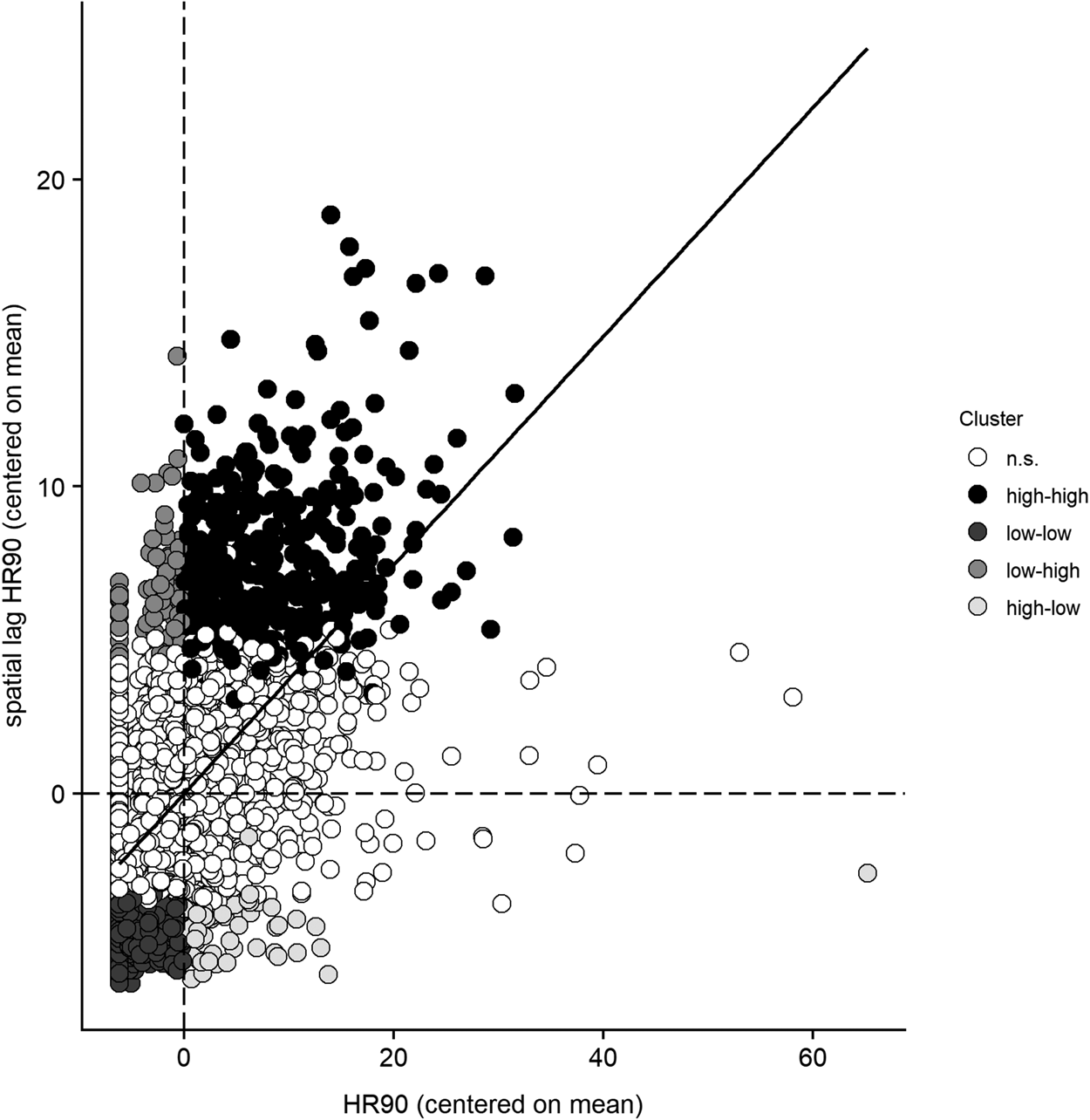
Fig 1. Moran scatterplot of outcome of interest (HR90)
The dashed lines divide the graph into quadrants. Starting from the upper left and moving clockwise, we observe: (1) dissimilar-values clusters of lower-than-average y and higher-than-average Wy (low-high clusters); (2) similar-values clusters of higher-than-average y and higher-than-average Wy (high-high clusters); (3) dissimilar values clustering of higher-than-average y and lower-than-average Wy (high-low clusters); and (4) similar values clustering of lower-than-average y and lower-than-average Wy (low-low clusters). Further, the association between y and Wy captured by the individual LISA values can be either statistically significant or non-significant. White circles identify focal units of cores that are not statistically significant, and all shaded circles identify cores of clusters that are statistically significant (p < 0.05). Overall, while the global Moran's I may suggest limited spatial autocorrelation in the data, LISA values can identify smaller, localized geographic areas where clustering occurs.
Complementing the Moran scatterplot, a series of LISA maps is often used to visualize these local features of association, visualizing the data in a more explicit geographic context. Building on Anselin (Reference Anselin1995: 106–107), we offer a systematic approach for using LISA statistics, clusters, scatterplots, and maps for case selection.
Option 1: LISA statistics of outcome of interest
With LISA tools in hand, how would a researcher proceed? Since LISA statistics and maps contain a lot of information, we suggest researchers proceed in four steps: (1) generate LISA scatterplot and maps; (2) evaluate scope conditions; (3) evaluate unit or level of analysis; (4) identify promising sites for in-depth research.
Step 1. Generate LISA scatterplot and maps. Figure 1 shows the relevant scatterplot, and Figure 2 shows six maps in three rows, translating the same data from the scatterplot in Figure 1 into a cartographic display. The top map on the left displays the raw homicide rates (HR90); the map to its right reports p-values for the LISA statistics. In this map, shaded areas indicate a statistically significant relationship between y (homicide rates) and the spatial lag (Wy) of homicide rates. The maps in the second row display the LISA values (positive values identifying similarity clusters on the left, and negative values identifying dissimilarity clusters on the right).Footnote 4 The third row contains two LISA cluster maps: the map on the left highlights similarity clusters (“high-high”, corresponding with top-right quadrant in Figure 1, indicating counties with higher-than-average homicide rates surrounded by counties with higher-than-average homicide rates, and “low-low”, corresponding with bottom-left quadrant in Figure 1) with dissimilarity clusters in background (light grey). The map on the right highlights spatial outliers or dissimilarity clusters (low-high and high-low) with similarity clusters now in the background (light grey). Spatial outliers or dissimilarity clusters come in two forms. First, “low-high” clusters, corresponding with top-left quadrant in Figure 1, reflect counties with lower than average homicide rates surrounded by counties with higher than average homicide rates. Conversely, “high-low” clusters, corresponding with bottom-right quadrant in Figure 1, indicate higher than average homicide rates locally and lower-than-average homicide rates in connected units. In the maps of p-values and LISA clusters, blank areas indicate spatial randomness in the distribution of violence (p > 0.05) while shaded areas are statistically significant spatial clusters (same as Figure 1).
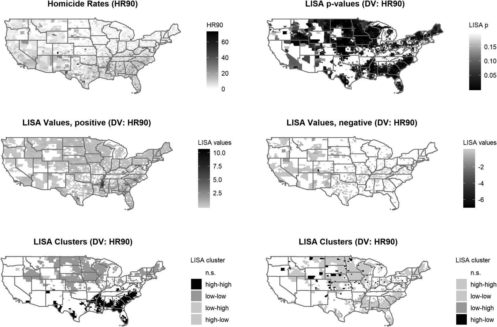
Fig 2. Maps of LISA statistics for option 1
Step 2. Scope Conditions: The second step is to explore whether the distribution of the dependent variable and the pattern of spatial association suggest the need to set scope conditions. The importance of defining the appropriate universe of cases and reflection on causal homogeneity across cases is well-documented in the literature on qualitative and mixed-method research. Broadly, concerns about causal heterogeneity can be addressed in two ways. First, scholars can seek to narrow the frame of comparison by delimiting specific domains or including scope restrictions so that the relationship of interest is homogenous across analyzed cases. Second, scholars can seek to uncover the substantive reasons for causal heterogeneity by identifying the factors that set groups of cases on distinct causal paths (Munck, Reference Munck, Brady and Collier2004:107–111; Seawright, Reference Seawright2016b). Case study scholars tend to be acutely aware of the need to choose the appropriate frame of comparison, especially since a too narrowly focused comparison incurs the risk of selection bias (Collier and Mahoney, Reference Collier and Mahoney1996). Thinking about causal heterogeneity from a spatial perspective can help mixed-methods scholars work through some of these challenges.
Specifically, the LISA maps provide an opportunity to examine local spatial instability (Anselin, Reference Anselin1995: 97). Such instability could suggest causal heterogeneity across observations, and would be indicated by regional heterogeneity in LISA statistics based on LISA values, their statistical significance, or cluster type. There may be large regions of one type of cluster or another, and there may also be regions of spatial randomness. Such instability points to the existence of heterogeneity or different geographically bounded regimes of spatial association. The geographic structure of these regimes may be more or less informative to a researcher possessing in-depth expertise or case knowledge, depending on their size or boundaries. If the pattern of spatial association varies, this suggests that the underlying process may also vary. Researchers can leverage this information to define the universe of cases.
Returning to our example, focusing on the third row in Figure 2, the first cluster map shows statistically significant clusters of high homicide rates across the South (black) and clusters of low homicide rates in the Upper Midwest and Northeast (grey). To illustrate the utility of the LISA statistic, let us imagine that a researcher was studying homicide across US counties for the first time and that knowledge of regional influences was yet unknown or uncertain; a map like the one in the bottom-left panel of Figure 2 would quickly signal that there was spatial component to the phenomenon, and could shape an entire research agenda. The overall higher incidence and spatial association of homicide in the South—clearly visible in the map—has prompted scholars to include a dummy for this region in quantitative studies of violence in the US. Displaying these patterns geographically allows us to connect information about our outcome of interest to more familiar geographic categories (e.g., state, region). The clusters suggest that there is something distinctive about the South compared to the rest of the country with regard to high violence, and there is something distinctive about the non-South with regard to low levels of homicide. This is not a pattern that would emerge as readily or visibly using non-spatial techniques, and recognizing such spatial heterogeneity can allow for better case selection. Scholars may want to select cases from units with similar causal processes to bolster confidence in causal homogeneity among the selected cases. Such a strategy would allow maximizing variation on the dependent variable to avoid concerns of selection bias (Collier and Mahoney, Reference Collier and Mahoney1996). Alternately, scholars can select cases with different causal processes to identify omitted variables.
Step 3. Unit selection and level of analysis. A third, related step is to examine how the outcome of interest maps onto existing administrative boundaries (e.g., states, counties, municipalities, electoral districts, legal jurisdictions) or physical boundaries (e.g., rivers, canyons, mountains). Mapping the outcome of interest with a series of LISA maps enables scholars to reflect on their chosen unit of analysis in relation to these boundaries, and reflect on the appropriate unit or level of analysis. In the current example, visible clusters extend beyond or straddle state boundaries, including high-violence clusters in the South and low-violence clusters across the upper Midwest. Analyzing these spatial patterns enables us to examine how formal state boundaries (and other jurisdictional limits of interest) succeed (or fail) in containing an outcome. If, as in our example, the outcome does not align with state lines, this suggests that states may not be the most useful unit of analysis and scholars may be better off exploring alternative units for in-depth study. The ability to explore the boundedness of what constitutes a “case” is one of the key advantages of spatial tools.
Step 4. Set selection based on LISA clusters: The fourth step is to identify promising locations for in-depth research by organizing observations by type of LISA cluster, and then sorting within each cluster type by LISA value and significance to identify locations that are emblematic or typical of each cluster. Building on our running example, Table 2 identifies the top five focal units per cluster type that would be promising sites for in-depth qualitative work. Recalling our earlier discussion of selecting units versus sets, we emphasize that Table 2 identifies focal units of clusters, so these observations should be examined alongside their neighbors to better understand the origins of similarity or dissimilarity. Similarity (high-high and low-low) and dissimilarity (low-high and high-low) clusters each reveal analytically interesting patterns, which raise questions for researchers about the origins of these patterns.
TABLE 2. Focal Units Selected Based on LISA Clusters
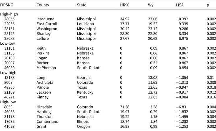
Similarity clusters could be the product of spread or diffusion from one unit to another, or a shared factor that explains similar levels of the outcome. Returning to our example to better understand why a particular location might be analytically interesting, selecting cases for further study from the South's collection of high-high clusters affords opportunities to examine why violence spreads from one place to another, or what common factor southern counties may be exposed to that results in elevated violence. For example, scholars have posited a “culture of violence” in the South (e.g., Nisbett Reference Nisbett1993), although its origins and content remain poorly understood and the mechanisms through which it is transmitted remain underspecified (Land et al., Reference Land, McCall and Cohen1990; Tolnay et al., Reference Tolnay, Deane and Beck1996). For scholars wishing to better understand this phenomenon, it would be helpful to select one or more high-high clusters (each consisting of a focal unit and its neighboring units) for in-depth study. Thus, the top observation within this cluster in Table 2—Issaquena County, Mississippi—would be a promising location in which to conduct qualitative research to analyze whether shared cultural factors across neighboring counties help explain the cluster. Interestingly, four out of the five counties that are cores of high-high clusters in Table 2 are from the same part of Mississippi, three of them are contiguous, and the fifth county—East Carroll, Louisiana—is contiguous to Issaquena but just across the state border. All of these counties are rural, so one could explore the hypothesis of a factor shared in common across all five counties, like weak institutions for conflict resolution. Ultimately, the spatial pattern provides leverage to scholars since it indicates the need to consider explanatory factors present across counties and state-lines.
It may be equally promising to examine a low-low cluster in order to uncover the sources of low violence in the Northeast and upper Midwest. Indeed, in their concluding remarks, the pattern of low-low clusters led Baller et al., to hypothesize that rather than focusing on a southern culture of violence, as much of social science had done, perhaps researchers should also study a shared “non-Southern culture of nonviolence” (583). However, rather than pointing to all of the non-South, the tools in Table 2 allow us to focus on specific observations. Again, the analytic goal is to identify either a mechanism of diffusion or a factor shared in common across connected units. The top observation among low-low clusters in Table 2 would be a promising location for fieldwork aimed at detecting shared factors inhibiting violence across neighboring counties. A researcher might find evidence that strong family or friendship networks inhibit violence, or that strong institutions shared across units inhibit violence. For instance, a study of robberies across more than 1,000 cities in the US found that city-level variation was influenced by an omitted variable shared across cities within the same state (Deane et al., Reference Deane, Messner, Stucky, McGeever and Kubrin2008, 376). In that study, authors hypothesized that such state-level factors could include legal factors (e.g., policing or other criminal justice practices) or political factors (e.g., ideology of dominant executive or legislative coalitions; 376–377). These are some of the factors researchers could inspect more closely as they conduct qualitative work in the locations in Kansas or Nebraska.
Dissimilarity clusters, by contrast, are interesting because they indicate within-case variation on the outcome of interest. The focal units defy regional patterns and differ significantly from their neighbors. What explains this variation? In our homicide data, two patterns can be distinguished in the bottom right cluster map: low-high clusters are scattered across the South (around the edges of the region of high-high clusters in the bottom left map) while high-low clusters are scattered across the North and Midwest (around the edges of the region of low-low clusters in the bottom left map). While the higher incidence of homicide in the South has led scholars to theorize about factors common to the region, these pockets of dissimilarity suggest pronounced within-region variation. Stated otherwise, there are spatial outliers across the South, where units with low homicide rates are surrounded by units with high homicide rates (low-high clusters). Similarly, there are high-low clusters in the North and Midwest; counties with statistically significant associations between high local homicide rates and low neighboring homicide rates. Examining counties in such dissimilarity clusters can provide analytic leverage to uncover why some counties are able to defy broader regional patterns.
For instance, Tolnay et al. (Reference Tolnay, Deane and Beck1996) argue that media markets might help explain why violence appears to concentrate spatially in only parts of the South in the early 20th century, positing that reports of lynchings in one part of a newspaper circulation market operated as a kind of signal or demonstration of white supremacy, suppressing additional lynchings by reducing white racial anxiety in nearby communities within the same media market. Similarly, Messner et al.’s (Reference Messner, Anselin, Baller, Hawkins, Deane and Tolnay1999) notion of “barrier counties” offers a useful heuristic; if diffusion is essentially a phenomenon of spatial homogeneity, then spatial outliers can be studied to understand barriers to homogeneity. Again, it is worth noting that these patterns would be difficult or impossible to see with non-spatial case selection techniques.
Option 2: LISA statistics (and maps) of residuals from baseline model
The LISA statistics in Figures 1 and 2 provide information about the spatial distribution of the outcome of interest. Another strategy for case selection is to generate LISA statistics on the basis of the residuals of a baseline regression model (Cliff and Ord, Reference Cliff and Ord1972; Anselin, Reference Anselin1988). This approach looks for the geographic structure in the error term and selects cases based on this structure. Specifically, the goal of case selection is to better understand what may be missing from the model and to uncover omitted variables by examining the performance of the model across space. Our discussion of option 2 moves faster since much of the conceptual and analytic tools from option 1 carry over.
Step 1. Generate LISA scatterplot and maps. Returning to our example, Baller et al., estimate a baseline least-squares model by regressing homicide rates on resource deprivation (RD90), population structure (PS90), median age (MA90), divorce rate (DV90), unemployment rate (UE90), and a dummy for the South. This model builds on previous research and constituted the state of the art in homicide research at the time of publication. All independent variables are significantly associated with homicide rates, and the model explains almost half of the variation in the data. We exclude the regional dummy in order to identify spatial patterns without the interference of a theoretically uninformative categorical variable, and extract the residuals (y − ŷ) from the model (mean of residuals is zero, so these are centered on zero).
We then repeat the procedures from option 1, this time generating LISA values, p-values, and clustering statistics using the residuals. This approach facilitates exploratory analysis of the spatial structure in the unexplained component of the model. Statistically significant clusters of either low or high residuals show the geographic structure in the error term, and this structure raises broader regional questions about shared exposure to an omitted common factor or a shared underlying process like spatial diffusion. We refer readers to the appendix for the Moran scatterplot of the residuals and focus on mapping the data.
Figure 3 contains seven maps in four rows. The two maps in the first row report the raw residuals (positive on left, negative on right). The two maps in the second row report LISA values for these residuals (positive and negative). The lone map in the third row reports the p-values for the LISA values in row two, and the fourth row shows LISA clusters.
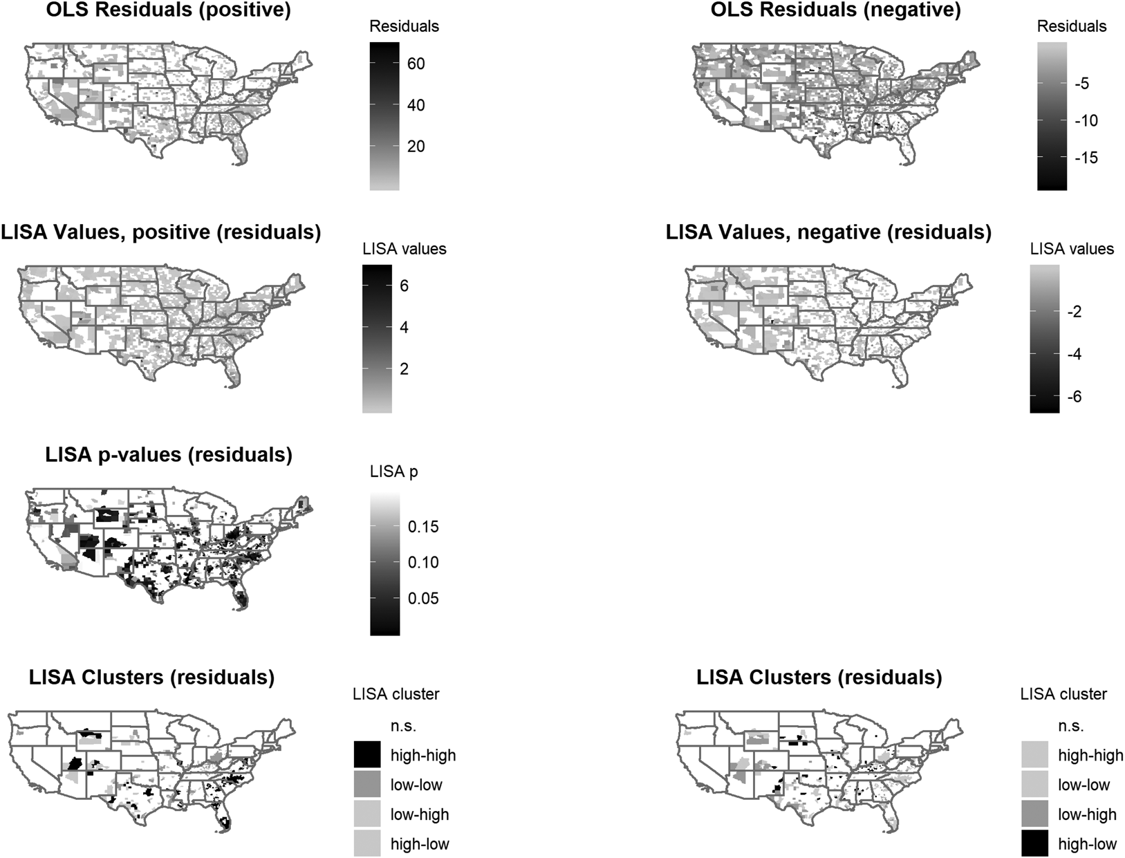
Fig 3. Maps of LISA statistics for option 2
Step 2. Scope conditions. The maps reveal the model's geographically uneven performance, with three general patterns: (1) areas with positive residuals (i.e., y − ŷ > 0, so y > ŷ) across the South and Southwest, indicating homicide rates higher than expected on the basis of the substantive predictors; (2) areas with negative residuals across much of the rest of the country (y − ŷ < 0, so y < ŷ), indicating homicide rates lower than predicted by the model; and (3) areas with low residuals (near zero, either positive or negative) where the model performs best. Depending on subject matter expertise or case knowledge, a researcher can use the geographic patterning of residuals to evaluate scope conditions.
Step 3. Unit or level of analysis. As was the case with option 1, the geographic patterning of residuals can also help assess the appropriateness of the unit or level of analysis. For instance, if residuals seem to follow the geographic structure of larger geographic boundaries, then the analyst may want to consider moving up a level. However, this pattern may also suggest an omitted variable at that higher level of analysis, which we turn to in the next section.
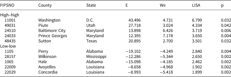
Step 4. Set selection based on LISA clusters. In Table 3 we organize observations by type of LISA cluster, and then sort within each cluster type by LISA value and significance to identify cases that are emblematic or typical of each cluster. Note that this strategy, which also relies on examining a “set”, suggests different locations for in-depth analysis than option 1.
TABLE 3. Locations Selected based on LISA Clusters of Residuals
The non-spatial mixed-methods literature recommends that scholars select high-residual, poorly predicted cases—“off the regression line”—to explore measurement error, generate new hypotheses, and identify previously omitted variables (Seawright, Reference Seawright2016b). Extending this logic to spatial studies, high-residual clusters (positive or negative) are particularly useful for building theory. As noted by King (Reference King1996), most analysts have an intuitive understanding of geography, so visualizing the spatial structure of the error component helps access such intuitions.
High-high clusters are analytically interesting because an unidentified local factor increases the incidence of homicide beyond what we would expect from the model, generating a statistically significant grouping of high, positive residuals; in low-low clusters, an unidentified factor has a dampening effect beyond what was expected based on the model, generating a significant grouping of large, negative residuals. Thus, the analytic goal of qualitative research in either type of location would be to identify these factors and generate new hypotheses. For example, researchers might select Washington County, D.C., and Prince George's County in Maryland, which are neighbors, as instances where the baseline model under-predicted homicide rates, prompting researchers to look for a factor that, all else being equal, might increase violence. Following the logic of Deane et al. (Reference Deane, Messner, Stucky, McGeever and Kubrin2008), the fact that these units are neighbors across state lines provides additional leverage by suggesting that the same factor might be present in both D.C. and Maryland, so fieldwork in these sites might focus on state-level factors common to both states, or a local factor such as criminal networks operating across state lines. Among low-low clusters, the units in Alabama are neighbors, and the observations in Louisiana and Mississippi are neighbors across state lines; these are study areas where the baseline model over-predicted homicide rates, prompting fieldwork to focus on identifying a factor that might dampen or reduce violence. Again following the logic of Deane et al. (Reference Deane, Messner, Stucky, McGeever and Kubrin2008), the clusters straddling state lines across Louisiana and Mississippi are particularly promising since researchers could start by looking for the same type of state-level factor across two state jurisdictions. In sum, researchers would be aiming to identify an omitted variable affecting a group of connected units, thereby giving substantive content to what might otherwise be characterized simply as “context.”
Combining options: a research example
While we have so far presented option 1 and 2 as distinct paths, they can also be combined fruitfully or sequenced in different ways. Which path is most promising naturally depends on the research problem at hand, and the state of previous theory and case knowledge. We illustrate one possibility for combination based on a real-world research example. Denton et al. (Reference Denton, Vesselinov, Deane and Raffalovich2001) examined the effect of racial composition on the change in housing value (i.e., housing appreciation) across census tracts in the metro area of Washington, D.C. After a regression analysis based on the state of the art in the literature failed to show satisfying statistical significance or model fit, suggesting an unexpectedly poor relationship between racial composition and housing values, the authors generated LISA maps of the outcome of interest, thus essentially deploying our option 1. Those LISA maps of the outcome identified six census tracts as spatial outliers, that is, as high-low clusters (tracts with higher-than-average appreciation surrounded by tracts with lower-than-average appreciation). The authors then conducted brief fieldwork in those areas to better understand why these units defied the regional pattern. Their “working hypothesis was that since these tracts were outliers in terms of the amount of appreciation or depreciation, there might be some characteristics of these neighborhoods not captured in census data that would explain them” (Denton et al., Reference Denton, Vesselinov, Deane and Raffalovich2001: 11). Identifying these characteristics and coding them for all neighborhoods would then yield a better statistical model, and contribute to theory development. The fieldwork generated two key insights. First, these tracts had major institutions (e.g., hospitals, universities, military bases) that generate a stable local demand for housing. Second, the level of socioeconomic development varied across these units, so that spatial outliers are neither uniformly rich nor poor. When Denton et al. (Reference Denton, Vesselinov, Deane and Raffalovich2001) included a dummy for the presence of institutions, the model fit increased dramatically and the statistical significance of racial composition now aligned with theoretical expectations. Moreover, the identification of the role of institutions in “anchoring” housing values contributed to the substantive understanding of the outcome of interest.
In this example, the authors began with a quantitative design, but failed to obtain satisfactory results. They then re-evaluated their statistical model, used LISA statistics of the outcome of interest to inform case selection for qualitative research, identified a plausible new explanatory variable, and then revised their quantitative modeling with the new information. In other words, Denton et al.’s (Reference Denton, Vesselinov, Deane and Raffalovich2001) approach allowed them to both (a) identify a previously omitted factor (institutional presence), and (b) rule out a potential confounder (socio-economic level). The visualization of the outcome of interest and statistics capturing local spatial association provides scholars with multiple opportunities to identify locations in which to conduct qualitative research to better understand how and why a phenomenon of interest is distributed unevenly across geographic space.
Another possibility for combining options 1 and 2 could take place in two steps. First, option 1 could lead to the development of distinct quantitative models for regions if option 1 suggests causal heterogeneity. Baller et al. (Reference Baller, Anselin, Messner, Deane and Hawkins2001) followed this strategy and separately modeled the South and the non-South. Subsequently, researchers could then run diagnostics from option 2 on the new models for each region, and proceed from there.
Conclusions
We have offered scholars two new options for studying why outcomes of interest are distributed unevenly across space by selecting promising locations in which to conduct qualitative research to uncover the origins of spatial patterns, focusing on identifying either (a) mechanisms of diffusion or (b) relevant omitted variables. The power of analyzing and presenting the data geographically, we argue, lies in the intuitive utility of maps for making sense of the social world. We therefore encourage mixed-methods scholars who currently only use non-spatial data to think about how they might leverage tools from spatial analysis.
Supplementary Material
The supplementary material for this article can be found at https://doi.org/10.1017/psrm.2019.3
Acknowledgments
Previous versions of this paper were presented at the 2016 and 2018 meetings of the American Political Science Association, at the 2016 meeting of the Southwest Mixed Methods Workshop, and as part of the Program Director Initiative Panel on “Spatial Models of Politics” at the 2017 meeting of the Southern Political Science Association. We thank discussants and participants at each meeting, especially Scott Cook, David Darmofal, Glenn Deane, Chris Hare, Philipp Hunziker, Ryan Saylor, Jason Seawright, Andrea Simpson, Hillel Soifer, and Laura Stoker. We gratefully acknowledge helpful feedback from the journal’s editor and anonymous reviewers. We thank the National Consortium on Violence Research (NCOVR) for making available the county-level homicide data (http://spatial.uchicago.edu/sample-data). Matthew Ingram acknowledges support from the Department of Political Science, the Rockefeller College of Public Affairs and Policy and the Center for Social and Demographic Analysis (CSDA) at the University at Albany, SUNY. Imke Harbers’ work on this project was partially funded by a Marie Curie Fellowship [Grant # 656361]. This paper is part of an ongoing project to which both authors contribute equally.


 Open access