


Introduction
According to a recent report (Vos et al., Reference Vos, Lim, Abbafati, Abbas, Abbasi, Abbasifard and Abdelalim2020), major depressive disorder (MDD) was ranked among the top 10 most disabling conditions across various age groups. Besides, the life expectancy for patients with depressive disorders is usually shorter than the general population due to both unnatural and natural causes of mortality (Kessler & Bromet, Reference Kessler and Bromet2013; Korhonen et al., Reference Korhonen, Moustgaard, Tarkiainen, Östergren, Costa, Urhoj and Martikainen2021; Vos et al., Reference Vos, Lim, Abbafati, Abbas, Abbasi, Abbasifard and Abdelalim2020). In recent years, genome-wide association studies (GWAS) and neuroimaging studies have advanced our understanding of the pathogenesis of MDD, although most advances have yet to be translated to clinical practice.
Precise classification of patients into more clinically and genetically homogeneous subgroups could facilitate our understanding of the underlying biological mechanisms and address the issue of phenotype heterogeneity (Yin et al., Reference Yin, Cheung, Chen, Wong, Sham and So2018; Yin, Chau, Sham, & So, Reference Yin, Chau, Sham and So2019). Importantly, it will also facilitate the discovery of subtype-specific treatments and promote individualized preventive and intervention strategies. In the extant literature, subtyping of patients with MDD mainly utilized clinical features only. The resultant MDD subtypes identified using clinical subtyping may not have distinct biological mechanisms. On the other hand, with the incorporation of genomic information and sophisticated subtyping methods, we may be able to stratify patients into more biologically homogenous subgroups. Nevertheless, limited research has applied genomic data for stratification of MDD patients.
Over the past two decades, substantial efforts have been made to dissect the genetic architecture of MDD (Howard et al., Reference Howard, Adams, Clarke, Hafferty, Gibson, Shirali and Wigmore2019; Major Depressive Disorder Working Group of the Psychiatric GWAS Consortium, 2013). Despite the substantial number of susceptibility loci identified from GWAS, translational applications remain scarce. One challenge is that the identified loci often reside in non-coding regions and may have only modest effects. To address this problem, here we employed a gene-based approach based on genotype-predicted expression changes, which is likely more biologically relevant and interpretable (Yin et al., Reference Yin, Chau, Sham and So2019) than SNP-based analysis. Of note, since the number of genes is large, preselection of relevant genes is common in many omics studies. However, most studies employed a univariate screening approach, yet a single gene may be associated with the outcome due to confounding (e.g. by other genes). Here we propose to employ a causal selection algorithm (PC-simple) (Bühlmann, Kalisch, & Maathuis, Reference Bühlmann, Kalisch and Maathuis2010) for gene selection, which may be considered a simplified version of the well-known PC algorithm (Kalisch & Bühlman, Reference Kalisch and Bühlman2007) for inferring causal features. We also propose to incorporate polygenic risk scores (PRS) of related disorders/traits for subtyping. PRS is a useful representation of the overall genetic predisposition of subjects to a disease by aggregating the effects of multiple variants (Murray et al., Reference Murray, Lin, Austin, McGrath, Hickie and Wray2021; Torkamani, Wineinger, & Topol, Reference Torkamani, Wineinger and Topol2018). While PRS has been widely applied in risk prediction studies, there have been very few applications in disease subtyping (Murray et al., Reference Murray, Lin, Austin, McGrath, Hickie and Wray2021; Torkamani et al., Reference Torkamani, Wineinger and Topol2018; Yin et al., Reference Yin, Chau, Sham and So2019).
Our main contributions are summarized below. Firstly, we present a new framework for neuropsychiatric disorder subtyping by integrating genotype-predicted expression profiles of relevant tissues, brain structural features, as well as other depression-related clinical features into a multi-view sparse bi-clustering model. The multi-view bi-clustering method is an unsupervised machine learning approach that allows multiple types of data to be considered simultaneously. Our work is unique in that we integrate brain imaging features (more specifically, grey matter volume in different brain regions) and whole-genome (imputed) transcriptome data for psychiatric disorder subtyping, which has not been attempted before. Compared with psychopathologies, neuroimaging characteristics are believed to be more directly reflecting the neuroanatomical basis of the disease. Another important novelty is that we incorporated a causal gene selection algorithm; owing to the causal selection approach, the identified subtype-defining gene-sets may be more functionally relevant to the underlying disease mechanisms.
Secondly, apart from methodological innovations, we applied our proposed framework to the study of MDD and revealed two subgroups of MDD with differing prognoses. Previous subtyping studies of MDD mostly focused on clinical features only and seldom integrated multiple sources of (high-dimensional) data for deriving patient subgroups (Van Loo et al., Reference Van Loo, De Jonge, Romeijn, Kessler and Schoevers2012). We identified two subgroups of MDD patients with divergent prognoses. The group with poorer prognosis is also characterized by reduced gray matter volume across multiple brain regions. In addition, we revealed genetic differences across the two subgroups and the pathways involved. We believe these findings are of both clinical interest and scientific importance.
Method
A novel disease subtyping/patient stratification model
In brief, our proposed framework comprised 4 stages, i.e. data imputation, feature selection, disease subtyping, and validation (as shown in Figure 1). Next, we shall describe each step in greater detail below.
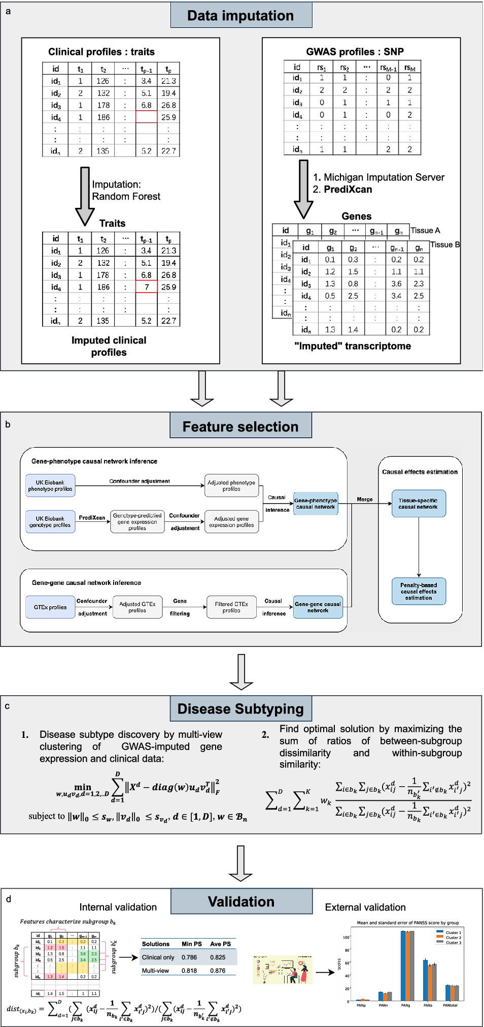
Figure 1. The workflow for the proposed invention in identifying disease subtypes.
Data imputation
Given that clustering analysis could not accommodate missing data, imputation was performed. Different methods were used to impute missing clinical and genetic features. For clinical data, the R package ‘missForest’ (Stekhoven & Bühlmann, Reference Stekhoven and Bühlmann2012) was employed to impute the missing data by a random forest algorithm. As for the estimation of expression profiles from GWAS, we employed ‘PrediXcan’ (Gamazon et al., Reference Gamazon, Wheeler, Shah, Mozaffari, Aquino-Michaels, Carroll and Cox2015) developed by Gamazon et al. to impute expression levels of relevant tissues from genotype data. The algorithm first built elastic-net-based prediction models with expression levels as the outcome from an external reference dataset (GTEx), which contained both genotype and expression data. Then, the developed prediction model was applied to new genotype data to estimate the expression levels in different tissues.
Feature selection by a causal approach
In this study, we proposed to use a gene-phenotype causal network inference method to identify causally relevant genes for the disorder of interest. Figure 1 shows the feature selection process. Confounder adjustments were separately performed for the disorder of interest and imputed expression profiles of the corresponding subjects. Specifically, we regressed the confounders separately against each imputed gene and phenotype. The residuals from these regressions were then used as adjusted gene expression and phenotype profiles in subsequent analyses.
In our primary analysis, we chose not to adjust for sex during feature selection. The main consideration is that our primary objective is to identify biologically and clinically homogenous subgroups, and sex itself is one of the major drivers of the biological differences in MDD. As such, we allow sex differences to emerge naturally in the clustering results. However, we recognize that a sex-adjusted analysis could provide complementary insights. For instance, one might wish to identify subtypes that are independent of sex, where clustering is driven by other genetic or clinical factors. Therefore, we also performed a subsidiary clustering analysis adjusted for sex.
The PC-simple algorithm (Bühlmann et al., Reference Bühlmann, Kalisch and Maathuis2010; Kalisch et al., Reference Kalisch, Mächler, Colombo, Maathuis and Bühlmann2012) was employed to infer the causal relationships between genes and the outcome, based on imputed expression profiles. In brief, PC-Simple can be regarded as a generalization of correlation screening that utilizes the ordered independence screening algorithm to estimate the causal relationships between genes and phenotypes. Intuitively, for each gene of interest, all subsets of other genes are controlled for, and those genes that remain significant will be kept as the set of ‘causal’ genes. A more detailed description is presented below.
Let $ X=\left[{X}^1,{X}^2,\dots {X}^p\right] $
be a
$ X=\left[{X}^1,{X}^2,\dots {X}^p\right] $
be a $ n\times p $
matrix of adjusted gene expression data for p genes, Y be a vector of the corresponding adjusted phenotype dataset for n subjects. Suppose Y is defined by a linear model of X, i.e.:
$ n\times p $
matrix of adjusted gene expression data for p genes, Y be a vector of the corresponding adjusted phenotype dataset for n subjects. Suppose Y is defined by a linear model of X, i.e.:
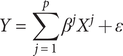 $$ Y=\sum \limits_{j=1}^p{\beta}^j{X}^j+\varepsilon $$
Where $ \varepsilon \sim N\left(0,\sum \right) $
denotes the noise item, and it is independent of
$ \varepsilon \sim N\left(0,\sum \right) $
denotes the noise item, and it is independent of $ {X}^j\left(j=1,2,\dots p\right) $
. For Equation (1), we believe most or some of the coefficients
$ {X}^j\left(j=1,2,\dots p\right) $
. For Equation (1), we believe most or some of the coefficients $ {\beta}^j $
are zero, while the remaining are nonzero for the studied phenotype. Our goal was to uncover the active gene set
$ {\beta}^j $
are zero, while the remaining are nonzero for the studied phenotype. Our goal was to uncover the active gene set $ G=\left\{j=1,2,\dots, p;\hskip0.3em ;{\beta}^j\ne 0\right\} $
with non-zero coefficients. Under the partial faithfulness assumption, we have:
$ G=\left\{j=1,2,\dots, p;\hskip0.3em ;{\beta}^j\ne 0\right\} $
with non-zero coefficients. Under the partial faithfulness assumption, we have:
 $$ \rho \left(Y,{X}^j|{X}^S\right)\ne 0\hskip0.3em for\hskip0.3em all\hskip0.3em S\subseteq {\left\{j\right\}}^C\; if\ and\ only\ if\;{\beta}^j\ne 0 $$
We could derive the active gene set through recursively performing partial correlation screening with increased order of conditional set based on (2) for all gene-phenotype pairs ( $ Y,{X}^j $
). Specifically, we first set the conditional set to null (
$ Y,{X}^j $
). Specifically, we first set the conditional set to null ( $ S=\varnothing $
) and obtained the first candidate gene set with non-zero correlations with our studied phenotype. Then we sequentially increased the order of the conditional set to eliminate irrelevant genes until the candidate gene set did not vary anymore. The partial correlations for each gene-phenotype pair can be estimated as follows:
$ S=\varnothing $
) and obtained the first candidate gene set with non-zero correlations with our studied phenotype. Then we sequentially increased the order of the conditional set to eliminate irrelevant genes until the candidate gene set did not vary anymore. The partial correlations for each gene-phenotype pair can be estimated as follows:
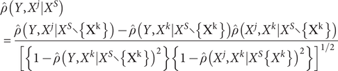 $$ \begin{array}{l}\hat{\rho}\left(Y,{X}^j|{X}^S\right)\\ {}=\frac{\hat{\rho}\left(Y,{X}^j|{X}^S\backslash \left\{{X}^k\right\}\right)-\hat{\rho}\left(Y,{X}^k|{X}^S\backslash \left\{{X}^k\right\}\right)\hat{\rho}\left({X}^j,{X}^k|{X}^S\backslash \left\{{X}^k\right\}\right)}{{\left[\left\{1-\hat{\rho}{\left(Y,{X}^k|{X}^S\backslash \left\{{X}^k\right\}\right)}^2\right\}\left\{1-\hat{\rho}{\left({X}^j,{X}^k|{X}^S\operatorname{}\left\{{X}^k\right\}\right)}^2\right\}\right]}^{1/2}}\end{array} $$
We tested partial correlations by Fisher’s Z-transform, which can be expressed as follows:
 $$ Z\left(Y,{X}^j|{X}^S\right)=\frac{1}{2}\left\{\frac{1+\hat{\rho}\left(Y,{X}^j|{X}^S\right)}{1-\hat{\rho}\left(Y,{X}^j|{X}^S\right)}\right\} $$
The null hypothesis ( $ \hat{\rho}\left(Y,{X}^j|{X}^S\right)=0 $
) is rejected if the following holds (Bühlmann et al., Reference Bühlmann, Kalisch and Maathuis2010):
$ \hat{\rho}\left(Y,{X}^j|{X}^S\right)=0 $
) is rejected if the following holds (Bühlmann et al., Reference Bühlmann, Kalisch and Maathuis2010):
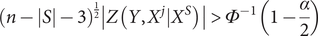 $$ {\left(n-\left|S\right|-3\right)}^{\frac{1}{2}}\left|Z\left(Y,{X}^j|{X}^S\right)\right|>{\varPhi}^{-1}\left(1-\frac{\alpha }{2}\right) $$
where $ \varPhi $
denotes the standard normal cumulative distribution function,
$ \varPhi $
denotes the standard normal cumulative distribution function, $ \alpha $
denotes the significance level for the null hypothesis test. In this study, we set
$ \alpha $
denotes the significance level for the null hypothesis test. In this study, we set $ \alpha =0.05 $
, the default setting in the original paper (Bühlmann et al., Reference Bühlmann, Kalisch and Maathuis2010). To boost the computational efficiency, we set the maximum order for partial correlation screening to 3. All genes that survived the 3-order partial correlation screening were regarded as directly causal genes for the studied phenotype. After deriving the tissue-specific gene-phenotype causal links for the studied phenotype, we could distinguish the directly causal genes from other ones, which would be included for the subsequent disease subtyping process.
$ \alpha =0.05 $
, the default setting in the original paper (Bühlmann et al., Reference Bühlmann, Kalisch and Maathuis2010). To boost the computational efficiency, we set the maximum order for partial correlation screening to 3. All genes that survived the 3-order partial correlation screening were regarded as directly causal genes for the studied phenotype. After deriving the tissue-specific gene-phenotype causal links for the studied phenotype, we could distinguish the directly causal genes from other ones, which would be included for the subsequent disease subtyping process.
Disease subtyping
For disease subtype discovery, we employed an extension of the biclustering algorithm in (Sun, Lu, Xu, & Bi, Reference Sun, Lu, Xu and Bi2015). In brief, we performed biclustering by matrix decomposition. Suppose $ {X}^d $
is a
$ {X}^d $
is a $ n\times {m}_d $
data matrix from the clinical or genetic view of patients, where n is the sample size,
$ n\times {m}_d $
data matrix from the clinical or genetic view of patients, where n is the sample size, $ d $
denotes the index of the ‘view’ to be modelled, and
$ d $
denotes the index of the ‘view’ to be modelled, and $ {m}_d $
is the number of features in the d th view. For example, if one models clinical and genotype-predicted expressions in one tissue, there will be two views. It is possible to extend the approach to more than two views, for example, based on expression in different tissues or using other (preferably gene-based) ‘omics’ profiles. It is worth emphasizing that due to the heterogeneity of patients, the pathophysiology (e.g. genetic pathways) underlying the disease may be different for different subgroups of patients. Using a biclustering algorithm, each bicluster can be characterized by different sets of gene features; in other words, we allow different genes to be involved for different subgroups of patients. This adds flexibility to our model and is an important advantage compared to ordinary clustering approaches.
$ {m}_d $
is the number of features in the d th view. For example, if one models clinical and genotype-predicted expressions in one tissue, there will be two views. It is possible to extend the approach to more than two views, for example, based on expression in different tissues or using other (preferably gene-based) ‘omics’ profiles. It is worth emphasizing that due to the heterogeneity of patients, the pathophysiology (e.g. genetic pathways) underlying the disease may be different for different subgroups of patients. Using a biclustering algorithm, each bicluster can be characterized by different sets of gene features; in other words, we allow different genes to be involved for different subgroups of patients. This adds flexibility to our model and is an important advantage compared to ordinary clustering approaches.
Subgroups of patients can be simultaneously derived by performing a sparse rank one approximation on the original matrices $ {X}^d $
(
$ {X}^d $
( $ d=1,2,..D $
, indicating data matrices from different views that characterize the same set of patients), i.e.
$ d=1,2,..D $
, indicating data matrices from different views that characterize the same set of patients), i.e.
 $$ {X}^d\approx \mathit{\operatorname{diag}}(w){u}_d{v}_d^T $$
where $ w $
is a binary vector of size
$ w $
is a binary vector of size $ n $
, serving as a common factor that forces different views of data to agree on the same grouping of patients.
$ n $
, serving as a common factor that forces different views of data to agree on the same grouping of patients. $ \mathit{\operatorname{diag}}(w) $
is a diagonal matrix of size
$ \mathit{\operatorname{diag}}(w) $
is a diagonal matrix of size $ n\times n $
with diagonal entries equal to
$ n\times n $
with diagonal entries equal to $ w. $ $ {u}_d $
of size
$ {u}_d $
of size $ n $
and
$ n $
and $ {v}_d $
of size
$ {v}_d $
of size $ {m}_d $
are the rank-one approximations of
$ {m}_d $
are the rank-one approximations of $ {X}^d $
respectively. Rows in
$ {X}^d $
respectively. Rows in $ {X}^d $
corresponding to the non-zero entries of
$ {X}^d $
corresponding to the non-zero entries of $ \mathit{\operatorname{diag}}(w) $
form the row subgroups, and columns in
$ \mathit{\operatorname{diag}}(w) $
form the row subgroups, and columns in $ {v}_d $
form the column subgroups (a.k.a., sub-feature groups) in different views. Subgroups of patients based on different views of data can be derived by solving the following optimization problem:
$ {v}_d $
form the column subgroups (a.k.a., sub-feature groups) in different views. Subgroups of patients based on different views of data can be derived by solving the following optimization problem:
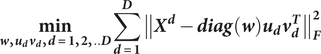 $$ \underset{\boldsymbol{w},{\boldsymbol{u}}_{\boldsymbol{d}}{\boldsymbol{v}}_{\boldsymbol{d}},\boldsymbol{d}=\mathbf{1},\mathbf{2},..\boldsymbol{D}}{\mathbf{min}}\sum_{\boldsymbol{d}=\mathbf{1}}^{\boldsymbol{D}}{\left\Vert {\boldsymbol{X}}^{\boldsymbol{d}}-\boldsymbol{\operatorname{diag}}\left(\boldsymbol{w}\right){\boldsymbol{u}}_{\boldsymbol{d}}{\boldsymbol{v}}_{\boldsymbol{d}}^{\boldsymbol{T}}\right\Vert}_{\boldsymbol{F}}^{\mathbf{2}} $$
subject to $ {\left\Vert \boldsymbol{w}\right\Vert}_{\mathbf{0}}\mathbf{\le}{\boldsymbol{s}}_{\boldsymbol{w}},{\left\Vert {\boldsymbol{v}}_{\boldsymbol{d}}\right\Vert}_{\mathbf{0}}\mathbf{\le}{\boldsymbol{s}}_{{\boldsymbol{v}}_{\boldsymbol{d}}},\boldsymbol{d}\mathbf{\in}\left[\mathbf{1},\boldsymbol{D}\right],\boldsymbol{w}\mathbf{\in }{\mathbf{\mathcal{B}}}_{\boldsymbol{n}} $
where
$ {\left\Vert \boldsymbol{w}\right\Vert}_{\mathbf{0}}\mathbf{\le}{\boldsymbol{s}}_{\boldsymbol{w}},{\left\Vert {\boldsymbol{v}}_{\boldsymbol{d}}\right\Vert}_{\mathbf{0}}\mathbf{\le}{\boldsymbol{s}}_{{\boldsymbol{v}}_{\boldsymbol{d}}},\boldsymbol{d}\mathbf{\in}\left[\mathbf{1},\boldsymbol{D}\right],\boldsymbol{w}\mathbf{\in }{\mathbf{\mathcal{B}}}_{\boldsymbol{n}} $
where $ {s}_w $
and
$ {s}_w $
and $ {s}_{v_d} $
’s are hyper-parameters that need to be predetermined to enforce sparsity of
$ {s}_{v_d} $
’s are hyper-parameters that need to be predetermined to enforce sparsity of $ w $
and
$ w $
and $ {v}_d $
’s, i.e. the number of patients
$ {v}_d $
’s, i.e. the number of patients $ {n}_{b_k} $
and number of selected features
$ {n}_{b_k} $
and number of selected features $ {n}_{v_k}^d $
in each subgroup of the corresponding data view.
$ {n}_{v_k}^d $
in each subgroup of the corresponding data view. $ D $
is the number of data views incorporated for clustering and
$ D $
is the number of data views incorporated for clustering and $ {B}_n $
is the set that contains all possible binary vectors of length
$ {B}_n $
is the set that contains all possible binary vectors of length $ n $
. To obtain subsequent subgroups, we need to first update the data matrices by excluding previously identified patients, and then solve Equation (7).
$ n $
. To obtain subsequent subgroups, we need to first update the data matrices by excluding previously identified patients, and then solve Equation (7).
Our proposed approach is capable of selecting features during the clustering process; however, we need to predetermine the number of selected features in each data view. Here we follow the suggestions given by the original authors (Sun et al., Reference Sun, Lu, Xu and Bi2015). Specifically, the number of selected features ( $ {n}_{v_k}^d $
) in each data view was set to the number where the accumulated variance after PCA of
$ {n}_{v_k}^d $
) in each data view was set to the number where the accumulated variance after PCA of $ {X}^d $
was over 90%.
$ {X}^d $
was over 90%.
The algorithm also requires the number and size of subgroups to be specified beforehand. We consider a value range of 2–6 for the number of subgroups, and the minimum number of subjects in each subgroup ( $ \min \left({n}_{b_k}\right) $
) was set to 20. This minimum subgroup size was chosen to balance between clinical utility, generalizability, and statistical separation. While smaller subgroups may show better mathematical separation, they are more prone to overfitting and may not be clinically meaningful or generalizable. Extremely small subgroups might represent outliers rather than true subtypes. Moreover, subgroups need to be large enough to allow for meaningful clinical characterization and potential validation in future studies. To assess the impact of this parameter, we also performed sensitivity analyses with smaller minimum subgroup sizes, as detailed below.
$ \min \left({n}_{b_k}\right) $
) was set to 20. This minimum subgroup size was chosen to balance between clinical utility, generalizability, and statistical separation. While smaller subgroups may show better mathematical separation, they are more prone to overfitting and may not be clinically meaningful or generalizable. Extremely small subgroups might represent outliers rather than true subtypes. Moreover, subgroups need to be large enough to allow for meaningful clinical characterization and potential validation in future studies. To assess the impact of this parameter, we also performed sensitivity analyses with smaller minimum subgroup sizes, as detailed below.
Suppose the number of subgroups is k, the size of each subgroup will be firstly set to a value roughly equal to $ n/k $
. Then all combinations by adding or subtracting
$ n/k $
. Then all combinations by adding or subtracting $ \min \left({n}_{b_k}\right) $
in each subgroup will be tried. A grid search approach was employed to determine the optimal solution. An evaluation metric is required to find the optimal solution. One of the most used metrics is mean squared residue (MSR). However, it only assesses the homogeneity within each subgroup and does not consider the heterogeneity between different subgroups. For well-separated subgroups, patients within the same subgroups should be highly homogenous, while patients belonging to different subgroups should be highly heterogeneous. In view of this, we employed the sum of ratios of the between-bicluster and within-bicluster distance (BBD/WBD) (Yin et al., Reference Yin, Chau, Sham and So2019) proposed by Yin et al. as the evaluation metric to identify the optimal solution.
$ \min \left({n}_{b_k}\right) $
in each subgroup will be tried. A grid search approach was employed to determine the optimal solution. An evaluation metric is required to find the optimal solution. One of the most used metrics is mean squared residue (MSR). However, it only assesses the homogeneity within each subgroup and does not consider the heterogeneity between different subgroups. For well-separated subgroups, patients within the same subgroups should be highly homogenous, while patients belonging to different subgroups should be highly heterogeneous. In view of this, we employed the sum of ratios of the between-bicluster and within-bicluster distance (BBD/WBD) (Yin et al., Reference Yin, Chau, Sham and So2019) proposed by Yin et al. as the evaluation metric to identify the optimal solution.
Validation
We employed external and internal validations (as shown in Figure 1) to verify our identified subtypes. Regarding external validation, this method was used when external data of disease outcomes were available (the disease outcome variables were not used for deriving the clusters). We evaluated whether disease outcomes were significantly different across the derived subgroups.
Regarding internal validation, here we utilized the extended ‘prediction strength’ (PS) method (Tibshirani & Walther, Reference Tibshirani and Walther2005) developed in our previous study (Yin et al., Reference Yin, Chau, Sham and So2019), which was designed for multi-view (bi-)clustering analysis to validate identified subgroups. Intuitively, this approach tests whether the derived clusters are generalizable to a new dataset. To calculate the PS, firstly we split the sample into a ‘training set’ and a ‘testing set’, and then evaluated whether the disease subtyping model derived from the training set could ‘predict’ the actual disease subgroups based on the testing set alone. In essence, it measured how well the ‘predicted’ co-memberships (based on the model derived from training set) matched with those in an independent testing set. In this study, we calculated both the ‘min PS’ and ‘ave PS’ to evaluate the performance of our proposed method. The ‘min PS’ and ‘ave PS’ respectively measured the lowest and average proportion of co-memberships among all identified subtypes, as follow:
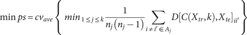 $$ \mathrm{min}\hskip0.3em ps=c{v}_{ave}\;\left\{\;{\mathit{\min}}_{1\le j\le k}\frac{1}{n_j\left({n}_j-1\right)}\sum \limits_{i\ne {i}^{\prime}\in {A}_j}D{\left[C\left({X}_{tr},k\right),{X}_{te}\right]}_{i{i}^{\prime }}\right\} $$
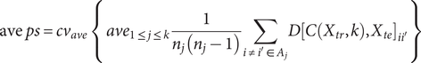 $$ \mathrm{ave}\hskip0.3em ps=c{v}_{ave}\;\left\{\;{ave}_{1\le j\le k}\frac{1}{n_j\left({n}_j-1\right)}\sum \limits_{i\ne {i}^{\prime}\in {A}_j}D{\left[C\left({X}_{tr},k\right),{X}_{te}\right]}_{i{i}^{\prime }}\right\} $$
Here $ C\left({X}_{tr},k\right) $
indicates the clustering operation on the training set with
$ C\left({X}_{tr},k\right) $
indicates the clustering operation on the training set with $ k $
subgroups.
$ k $
subgroups. $ D{\left[C\left({X}_{tr},k\right),{X}_{te}\right]}_{i{i}^{\prime }} $
denotes the co-membership for subjects
$ D{\left[C\left({X}_{tr},k\right),{X}_{te}\right]}_{i{i}^{\prime }} $
denotes the co-membership for subjects $ i $
and
$ i $
and $ {i}^{\prime } $
in subgroup
$ {i}^{\prime } $
in subgroup $ {A}_j $
.
$ {A}_j $
. $ {n}_j $
is the number of subjects in subgroup
$ {n}_j $
is the number of subjects in subgroup $ {A}_j $
.
$ {A}_j $
. $ c{v}_{ave} $
refers to the average of all cross-validation folds. Tibshirani and Walther (Reference Tibshirani and Walther2005) suggested that a PS of 0.8 or 0.9 or above indicates a reasonably good prediction strength.
$ c{v}_{ave} $
refers to the average of all cross-validation folds. Tibshirani and Walther (Reference Tibshirani and Walther2005) suggested that a PS of 0.8 or 0.9 or above indicates a reasonably good prediction strength.
Permutation testing of prediction strength
To rigorously evaluate the possibility of a single-cluster solution, we conducted a permutation test to assess the statistical significance of the observed prediction strength (PS) for the identified clustering solution. Under the null hypothesis of a single, homogeneous cluster, we generated a null distribution by independently permuting the values within each feature column. This procedure disrupts any existing relationships between features and subjects, effectively simulating the null scenario. The permutation p-value was then calculated as the proportion of permutations yielding a PS value greater than or equal to the observed PS.
Evaluation of minimum subgroup size on clustering analysis
To evaluate the influence of the minimum subgroup size on the identified subgroups, we conducted additional sensitivity analyses by relaxing the minimum subgroup size to 10 and 5. Clustering performance was assessed using within- and between-cluster distances (specifically, BBD/WBD ratio). We hypothesize that while cluster separation (e.g. as measured by BBD/WBD ratio) may be better with smaller minimum subgroup sizes, this might be attributable to overfitting. Consequently, we predicted that the stability and generalizability of the clustering solution would be reduced with smaller minimum subgroup sizes. To test this, we computed prediction strength for solutions with minimum subgroup sizes of 10 and 5.
To further evaluate the minimum subgroup size, we also performed a bootstrap-based stability analysis, following the approach by Yu et al. (Reference Yu, Chapman, Di Florio, Eischen, Gotz, Jacob and Blair2019). The stability of different clustering solutions was assessed using the Adjusted Rand Index (ARI) (Zhang, Wong, & Shen, Reference Zhang, Wong and Shen2012), a widely used metric for comparing clustering solutions. We employed bootstrap resampling (100 iterations) to calculate the co-membership matrix for each clustering solution. The co-membership matrix represents the proportion of times each pair of subjects is clustered together across the bootstrap samples. The ARI was then used to quantify the similarity between the co-membership matrix derived from the bootstrapped data and that derived from the original clustering solution.
Further analyses to evaluate the relevance of the subtype-defining genes
To further validate the identified subgroups, we examined whether genes selected by our proposed approach were enriched for GWAS hits for depression. Specifically, the GWAS summary statistics for depression (Howard et al., Reference Howard, Adams, Clarke, Hafferty, Gibson, Shirali and Wigmore2019) were first converted to gene-based statistics by FASTBAT (Bakshi et al., Reference Bakshi, Zhu, Vinkhuyzen, Hill, McRae, Visscher and Yang2016), then we tested whether the genes selected by our clustering framework had lower p-values than the non-selected ones.
In addition, we extracted genes selected by our method to figure out the genetic underpinning of each identified depression subtype. We then investigated whether there were significant differences in the expression profiles for these selected genes across the subgroups. Specifically, we employed both the default ‘t.test’ function in R and the ‘eBayes’ function from the R package ‘limma’ (Smyth, Reference Smyth2004) to detect differentially expressed genes (DEGs). Pathway analyses (based on hypergeometric tests) were also conducted using ‘ConsensumPathDB’ (Kamburov et al., Reference Kamburov, Pentchev, Galicka, Wierling, Lehrach and Herwig2011; Kamburov, Stelzl, Lehrach, & Herwig, Reference Kamburov, Stelzl, Lehrach and Herwig2013) to further explore the biological mechanisms. Furthermore, we conducted drug enrichment analyses on ‘Enrichr’ (Kuleshov et al., Reference Kuleshov, Jones, Rouillard, Fernandez, Duan, Wang and Lachmann2016) to identify repositioning candidates for each subtype.
Application to depression patients
We applied our disease subtyping model to depression subjects in the UK BioBank (UKBB). Here depression is defined by a combination of ICD-10 coded and self-reported disease. Since high missing rates may affect the imputation accuracy, we only keep patients with a comparably lower missing rate. It has been suggested that ~10% is a reasonable missingness cutoff, below which satisfactory imputation accuracy can be expected (Dong & Peng, Reference Dong and Peng2013; Madley-Dowd, Hughes, Tilling, & Heron, Reference Madley-Dowd, Hughes, Tilling and Heron2019). Following this, we only keep patients with variable missing rates less than 10%. Specifically, we included a variety of clinical features, including demographic/socioeconomic factors, mental health factors (especially symptoms related to depression), behavioral factors, medical history, and current health status (in particular cardiometabolic abnormalities) (Murray et al., Reference Murray, Lin, Austin, McGrath, Hickie and Wray2021; Torkamani et al., Reference Torkamani, Wineinger and Topol2018), for the subtyping analysis. Please refer to Supplementary Table S1 for all features. 13Besides, we estimated the expression levels for the cortex, frontal cortex, nucleus accumbens (basal ganglia), and putamen (basal ganglia) by ‘PrediXcan’ (Gamazon et al., Reference Gamazon, Wheeler, Shah, Mozaffari, Aquino-Michaels, Carroll and Cox2015) for all subjects with available genotypes. Previous studies suggested involvement of these brain regions in the pathophysiology of depression (Hare & Duman, Reference Hare and Duman2020; Lacerda et al., Reference Lacerda, Nicoletti, Brambilla, Sassi, Mallinger, Frank and Soares2003; Pandya, Altinay, Malone, & Anand, Reference Pandya, Altinay, Malone and Anand2012; Pizzagalli et al., Reference Pizzagalli, Holmes, Dillon, Goetz, Birk, Bogdan and Fava2009; Stockmeier & Rajkowska, Reference Stockmeier and Rajkowska2022; Zhang et al., Reference Zhang, Peng, Sweeney, Jia and Gong2018).
Besides, we also calculated PRSs of related neuropsychiatric traits/disorders. The traits for constructing PRS included autism spectrum disorder (ASD; N = 46,350) (Grove et al., Reference Grove, Ripke, Als, Mattheisen, Walters, Won and Anney2019), attention deficit hyperactivity disorder (ADHD; N = 53,293) (Demontis et al., Reference Demontis, Walters, Martin, Mattheisen, Als, Agerbo and Bækvad-Hansen2019), schizophrenia (SCZ; N = 105,318) (Pardiñas et al., Reference Pardiñas, Holmans, Pocklington, Escott-Price, Ripke, Carrera and Hamshere2018), bipolar disorder (BP; N = 41,653) (Ruderfer et al., Reference Ruderfer, Ripke, McQuillin, Boocock, Stahl, Pavlides and Loohuis2018), MDD (N = 500,199) (Howard et al., Reference Howard, Adams, Clarke, Hafferty, Gibson, Shirali and Wigmore2019) and post-traumatic stress disorder (PTSD; N = 200,000) (Nievergelt et al., Reference Nievergelt, Maihofer, Klengel, Atkinson, Chen, Choi and Gelernter2019). GWAS summary statistics were downloaded from the Psychiatric Genomics Consortium (PGC) (https://www.med.unc.edu/pgc) and The Integrative Psychiatric Research project (iPSYCH).
Before the standard PRS analysis, LD-clumping was required. In this application, we performed LD-clumping at $ {r}^2=0.1 $
within a distance of 1000 Kb (Choi & O’Reilly, Reference Choi and O’Reilly2019). PRS was generated by PRsice with a P-value threshold of 0.1. We incorporated these 6 PRSs as clinical features. In total, we included 69 depression-related clinical features, 139 brain structural features (volume of grey matter of different brain regions) and 6 PRSs of related neuropsychiatric disorders as input features in the clinical view.
$ {r}^2=0.1 $
within a distance of 1000 Kb (Choi & O’Reilly, Reference Choi and O’Reilly2019). PRS was generated by PRsice with a P-value threshold of 0.1. We incorporated these 6 PRSs as clinical features. In total, we included 69 depression-related clinical features, 139 brain structural features (volume of grey matter of different brain regions) and 6 PRSs of related neuropsychiatric disorders as input features in the clinical view.
Results
Overview and identification of causal genes
We extracted 28,335 depression subjects as cases and 285,921 as controls from UKBB as the input for the causal inference-based feature selection. To avoid possible biases introduced by population structure, we adjusted the predicted tissue-specific expression profiles and phenotype data by the top 10 principal components (PCs) of the corresponding genotype dataset first. Then we used the corrected input data to identify causally relevant genes for depression in each tissue. We identified 108, 101, 94, and 76 genes for cortex, frontal cortex, nucleus accumbens basal ganglia, and putamen basal ganglia, respectively. These genes were included as input in the corresponding genetic views for the subtyping of depression patients. In the clustering analysis, we included 352 depression patients with available brain imaging data for subtyping.
Feature selection and data view composition
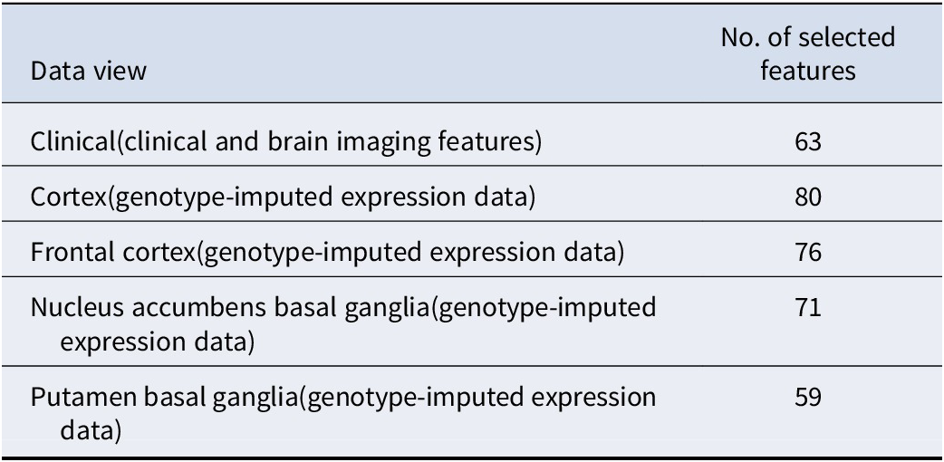
We incorporated 5 different views for the subtyping of depression patients: one clinical view with 139 brain structural features and PRS of 6 related disorders, and 4 genetic views corresponding to 4 brain regions with predicted expression profiles of causally relevant genes. As mentioned earlier, PCA was employed to determine the number of selected features in each data view. Table 1 lists the number of selected features in the corresponding data view.
Table 1. The number of selected features in each data view
Identification of two distinct depression subgroups
The best performance was achieved when the depression subjects were stratified into 2 different subgroups with 20 subjects in the first subgroup and 332 subjects in the second subgroup (Supplementary Figure S1). For clinical features, 63 out of 145 features were selected as subtype-defining features (see Table 1), and all of them were brain structural features (Supplementary Table S2). Table 2 summarizes the top 20 most significantly different (defined by the derived p-values from the t-test by comparing the brain volumes of the 2 subgroups) subtype-defining clinical features. We observed significant differences in selected features between the two identified subgroups (Figure 2 and Supplementary Table S2). Notably, among the selected subtype-defining brain structural features, most were shared in two subtypes. Significant differences in gene expression levels were observed on some of the identified subtyping-defining genes using limma (Table 3). Similar results were observed using a t-test for differential expression analysis (Supplementary Table S3).
Table 2. The 20 brain imaging features with the most significant differences (ranked by p-value) between the 2 discovered MDD subtypes
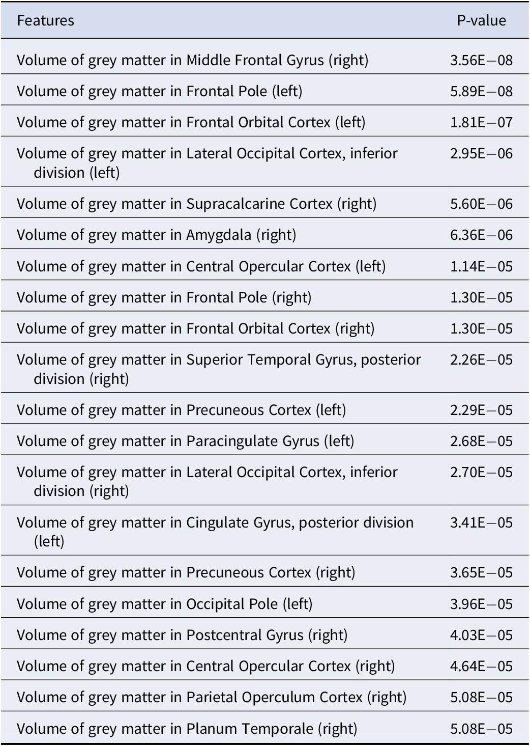

Figure 2. Comparison of selected brain imaging features for depression patients between 2 subtypes.
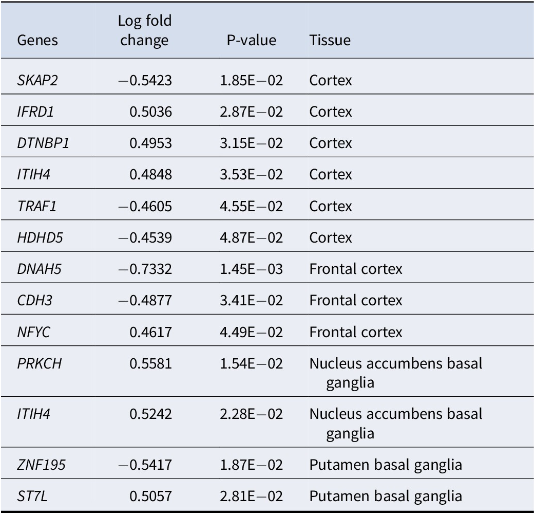
Table 3. Differentially expressed genes(DEGs) between the 2 depression subtypes, analyzed using limma (with gene expression in subgroup one as baseline)
Clinical validation: treatment resistance and psychiatric admissions
Using the UKBB, we gathered prognosis-related variables for these depression subjects. More specifically, we extracted the treatment resistance status and admission frequency of corresponding patients from the general practitioner (GP) records to evaluate our identified depression subtypes. In this study, treatment-resistance depression (TRD) was defined as MDD patients who tried at least two different antidepressant drugs for adequate durations (Fabbri et al., Reference Fabbri, Hagenaars, John, Williams, Shrine, Moles and Free2021). Following the definition in ref (Fabbri et al., Reference Fabbri, Hagenaars, John, Williams, Shrine, Moles and Free2021), the time interval between two drugs should be no longer than 14 weeks, and each drug should be prescribed for at least 6 weeks.
Since the medication records are not available for all subjects in the UKBB, we only gathered the treatment resistance status for 292 patients. When comparing the differences in TRD between the two derived subgroups, patients with missing values were excluded. Fisher’s exact test was performed to examine whether there exist significant differences between the two derived subgroups for the missing rate of drug records. Notably, we did not find any significant differences between the two subgroups in accessibility of patient records for TRD status (p = 0.356). We observed significant differences in TRD between the two derived subgroups using a regression model (higher rates of TRD in subgroup 2, p = 0.049) (Figure 3).
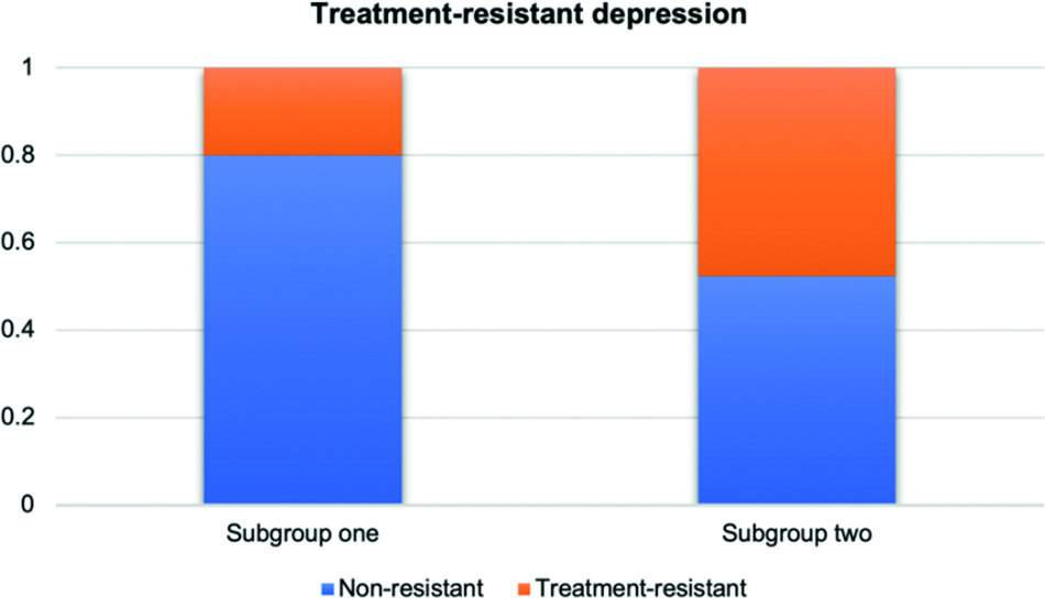
Figure 3. Comparison of TRD status by subgroups for depression patients.
Moreover, we compared the differences in psychiatric admission frequencies across the two derived subgroups using the Wilcoxon signed rank test. In line with TRD, subjects with missing values were excluded. The admission frequency records for 307 patients were available for further analysis. No significant difference was observed in the availability of patients’ records for psychiatric admissions across the two subgroups (Fisher exact test, p-value = 0.730). Again, we observed a significant difference in hospitalization frequencies between the two subgroups (p = 0.033) (Figure 4).
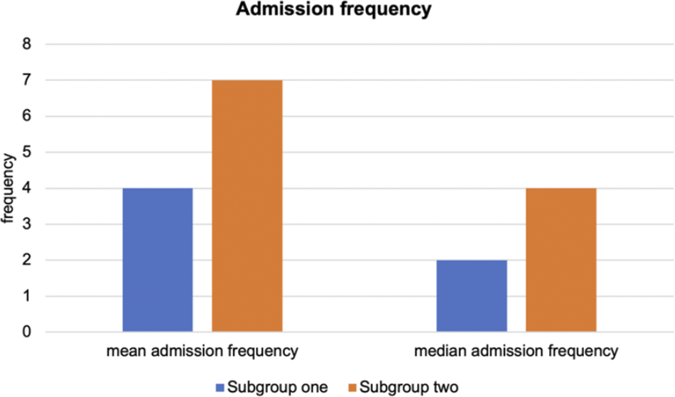
Figure 4. Comparison of admission frequencies by subgroups for depression patient.
Prediction strength
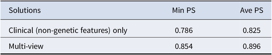
Furthermore, we computed the extended prediction strength (PS) of our identified 20–332 solution and observed a minimum PS of 0.854 and an average PS of 0.896 (Table 4). According to (Tibshirani & Walther, Reference Tibshirani and Walther2005), a PS of > = 0.8 or 0.9 suggests strong stability of the clustering model and good generalizability to new datasets. Therefore, we could conclude that our proposed method is reliable and stable in revealing depression subtypes. Moreover, we compared our method with clinical variable-based disease subtyping, which only relies on non-genetic features. Table 4 shows that our proposed method, which also integrates whole-genome (GWAS-imputed) transcriptome data, achieved higher ‘min PS’ and ‘average PS’ than the clinical variable-only subtyping method.
Table 4. Comparison of extended PS derived from different solutions
Beyond the overall PS, we performed additional analyses to validate our findings. First, the PS for the 20–332 solution was significantly higher than expected under a single, homogenous cluster (p = 0.010) based on permutation, providing strong evidence for the existence of distinct subgroups. Second, following the principles of PS and using the clustering model derived from the training set only, we tested for differences in treatment-resistant depression (TRD) across the identified subgroups in the test set. We observed significant differences in TRD (p = 0.042), further supporting the clinical relevance and generalizability of our identified subtypes.
Summary of evidence supporting distinct subgroups
To summarize, evidence strongly suggests that a two-cluster solution more accurately represents the data than a single-cluster model. This conclusion is supported by significant differences in clinical outcomes and biological markers (gene expression and imaging features) across the subgroups and permutation tests demonstrating that the prediction strength of the two-cluster solution significantly exceeds what would be expected under a single-cluster null hypothesis (p < 0.05).
GWAS enrichment analysis
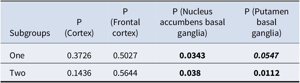
We downloaded the GWAS summary statistic for depression from PGC (Howard et al., Reference Howard, Adams, Clarke, Hafferty, Gibson, Shirali and Wigmore2019) to examine whether our selected genes were enriched for GWAS hits. Table 5 shows the enrichment analysis results. As expected, the genes picked up by our proposed framework were indeed enriched for known genes for depression. More specifically, subtype-defining genes for nucleus accumbens basal ganglia and putamen basal ganglia were significantly enriched for GWAS hits of depression.
Table 5. Enrichment analysis results for GWAS hits of depression
Functional annotation and pathway enrichment
Supplementary Table S3 demonstrates the subtype-defining gene sets identified by our proposed framework. Many selected (subtype-defining) genes were well-known susceptibility genes for depression or involved in the related pathophysiological process. For example, DTNBP1, NFYC, and PRKCH were selected by our algorithm as subtype-defining genes and showed differential expression across subtypes. Arias et al. (Reference Arias, Serretti, Mandelli, Gastó, Catalan, De Ronchi and Fananas2009) highlighted a significant association between DTNBP1 and responsiveness to antidepressants in MDD patients. Kocabas et al. (Reference Kocabas, Antonijevic, Faghel, Forray, Kasper, Lecrubier and Noro2010) corroborated this finding, citing its involvement in synaptic signaling and plasticity in patients with MDD. In another study, Fabbri and Serretti (Reference Fabbri and Serretti2016) demonstrated that NFYC was predictive of the depressive episode frequency in bipolar patients. Wong, Dong, Maestre-Mesa, and Licinio (Reference Wong, Dong, Maestre-Mesa and Licinio2008) revealed that PRKCH can affect the treatment response of MDD patients through dysregulating T cell and hypothalamic–pituitary–adrenal axis functions. For more details, please refer to Supplementary Table S3.
Supplementary Table S4 lists the top enriched pathways that characterize the identified disease subtypes. Numerous enriched pathways were involved in depression or related pathophysiology. Again, some enriched pathways were shared among two identified subtypes, while others were subtype-specific. Here we highlighted a few pathways that may be of interest. Regulation of PTEN stability and activity and tyrosine metabolism were found to be significantly enriched for depression patients. As suggested by Wang et al. (Reference Wang, Zhang, Xia, Chen, Fang and Ding2021), regulation of PTEN stability and activity could lead to an increase in depression-related behaviors in mice. Tyrosine metabolism might be related to anhedonia, a core symptom of depression, according to a recent study by Bekhbat et al. (Reference Bekhbat, Treadway, Goldsmith, Woolwine, Haroon, Miller and Felger2020). They also suggested that this pathway defined a subtype of depression with high C-reactive protein (CRP) and anhedonia. A study by Matsuda et al. (Reference Matsuda, Ikeda, Murakami, Nakagawa, Tsuji and Kitagishi2019) suggested that the ‘PIP3 activates AKT signaling’ pathway plays a critical role in the survival of various neurons, which may be implicated in depression-related behaviors. Chu et al. (Reference Chu, Wei, Zhu, Shen and Xu2017) reported that prostaglandin (PG) synthesis and regulation could lead to the onset of depression through downregulating PG D2 levels in the plasma. For more details about other enriched pathways, please refer to Supplementary Table S4.
Drug enrichment analysis
Supplementary Table S5 summarizes the enriched drugs for each identified depression subtype. Many were supported by previous studies for reversing depression-related symptoms or behaviors. For example, apigenin, and kaempferol were ranked among the top 5 enriched drugs for subtype 1 and valproic acid was ranked among the top 5 for subtype 2 (based on imputed expression in the cortex). Weng et al. (Reference Weng, Guo, Li, Yang and Han2016) found that apigenin could reverse depression-like behaviors in mice. Silva dos Santos, Goncalves Cirino, de Oliveira Carvalho, and Ortega (Reference Silva dos Santos, Goncalves Cirino, de Oliveira Carvalho and Ortega2021) reported that kaempferol, a flavonoid antioxidant, has a multipotential neuroprotective effect on depression. Valproic acid is a standard treatment for bipolar disorder and has been shown to be effective for bipolar depression (Smith et al., Reference Smith, Cornelius, Azorin, Perugi, Vieta, Young and Bowden2010). For more details on the corresponding enriched drugs, please refer to Supplementary Table S5.
Evaluation of smaller minimum subgroup sizes
Several sensitivity analyses were conducted to evaluate the influence of the minimum subgroup size on the identified subgroups (Table 6).
Table 6. Comparison of clustering solutions with varied minimum subgroup sizes
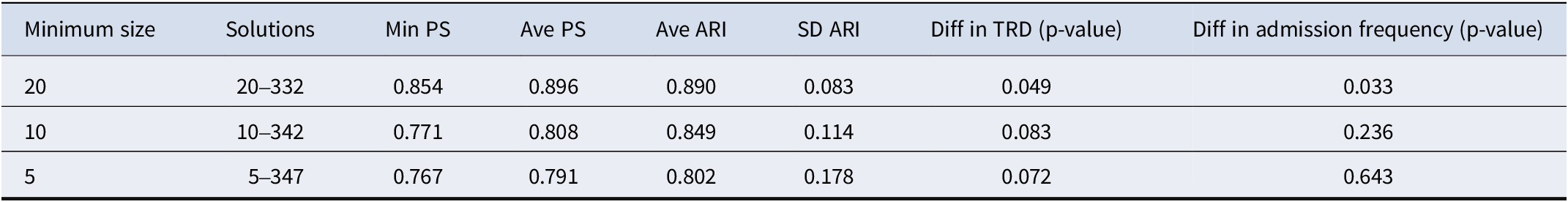
Notes: Min is the abbreviation for minimum, Ave is the abbreviation for average, SD is the abbreviation for standard deviation. ARI ranges between (−1,1), with ARI = 1 indicates perfect agreement between two clustering, ARI = 0 indicates no better than random agreement, ARI < 0 indicates worse than random agreement, TRD is the abbreviation for treatment resistance depression. For the clustering analysis with minimum subgroup size of 10 and 5, we employed Fisher’s exact test to compare the differences in TRD between the derived subgroups.
Prediction strength
While better BBD/WBD ratios were achieved with a minimum subgroup size at 10 or 5, subtyping solutions derived with smaller minimum subgroup sizes exhibited inferior prediction strength (PS) (Table 6), suggesting reduced generalizability and possible overfitting. The 20–332 cluster solution represents the solution achieving the best separation (as indicated by the BBD/WBD ratio), while having an average PS > = 90% (rounded to the nearest integer).
Bootstrap-based stability analysis
The stability of different clustering solutions was assessed with bootstrap resampling and ARI. Compared to solutions with smaller minimum subgroup sizes, the original solution with a minimum subgroup size of 20 exhibited significantly greater model stability and generalizability, as evidenced by a high ARI (0.89) and low SD of ARI across the bootstrap samples.
Differences in clinical outcomes
For subgroups derived with minimum subgroup sizes of 10 or 5, we did not observe significant differences in clinical outcomes (all p > 0.05), including treatment resistance and admission frequencies.
In summary, the 20–332 solution demonstrated a balance of optimal clustering performance, model stability, and generalizability. External validation confirmed the clinical relevance of the identified subgroups, with significant differences observed in clinical outcomes.
Sex-adjusted clustering analysis
We performed an additional clustering analysis adjusting for sex as a covariate. We identified 331, 293, 346, and 271 genes in the cortex, frontal cortex, nucleus accumbens basal ganglia, and putamen basal ganglia, respectively, as relevant features. Similar to our primary analysis, the optimal solution stratified subjects into two subgroups (20 and 332 subjects). The concordance of cluster labels between the sex-adjusted and original solutions was high for the larger subgroup (97.0%), though lower for the smaller subgroup (50%). The sex-adjusted analysis identified more subgroup-defining genes, which may be due to potentially better statistical power in covariate-adjusted models (Jiang et al., Reference Jiang, Kulkarni, Mallinckrodt, Shurzinske, Molenberghs and Lipkovich2017).
The derived subgroups from the sex-adjusted analysis showed distinct clinical outcomes. Specifically, significant differences in treatment-resistant depression (TRD) (p = 0.034) and hospitalization frequencies (p = 0.046) were observed between the subgroups (Supplementary Figures S2 and S3), mirroring the findings of our primary analysis. Furthermore, no significant differences in TRD or hospitalization frequencies were observed between the subgroups derived from the original and the sex-adjusted clustering solutions. These results suggest that adjusting for sex does not fundamentally alter the identification of clinically relevant MDD subgroups in our dataset. Detailed results are provided in the Supplementary Information (see Supplementary Tables S3e–i).
Clustering with principal components as input
We also conducted clustering analysis using principal components (PCs) accounting for >90% variance in each view as input. While this approach captured more variance, the resulting subgroups did not show significant differences in clinical outcomes (Supplementary Table S6). Therefore, our original approach of using PCA to select features directly may be more effective for identifying clinically distinct MDD subgroups. Please refer to the supplementary information for details.
Discussion
In this proof-of-concept study, we proposed a novel framework to identify depression subtypes by incorporating both clinical (primarily brain structural phenotypes) and genetic information. To the best of our knowledge, it is the first study to integrate (1) brain structural (imaging) data; (2) whole-genome (GWAS-imputed) transcriptome data; (3) depression-related clinical features; and (4) a causal algorithm of gene selection into a multi-view clustering framework for subtyping complex diseases.
Key findings and biological relevance
We demonstrated the validity of our proposed framework by applying it to MDD subjects extracted from the UKBB. Two different depression subtypes with significant differences in treatment resistance status and hospitalization frequencies were identified. More precisely, we found one subgroup with a good prognosis and another subgroup with a relatively poorer prognosis. Notably, we found that subgroup 2, the group with poorer prognosis, is characterized by reduced gray matter volumes across multiple brain regions. This finding corroborates previous studies (Ancelin et al., Reference Ancelin, Carrière, Artero, Maller, Meslin, Ritchie and Chaudieu2019; Hellewell et al., Reference Hellewell, Welton, Maller, Lyon, Korgaonkar, Koslow and Grieve2019; Wise et al., Reference Wise, Radua, Via, Cardoner, Abe, Adams and de Azevedo Marques Périco2017) also showing decreased gray matter volume in patients with depression or severe depression. For example, Hellewell et al. (Reference Hellewell, Welton, Maller, Lyon, Korgaonkar, Koslow and Grieve2019) showed replicable gray matter volume losses in various brain regions (such as cingulate gyrus, middle frontal gyrus) for MDD patients compared to normal subjects.
Internal validation (by PS) also supported the stability of our proposed method in revealing depression subtypes and satisfactory generalizability to new datasets. Furthermore, the subtype-defining genes were significantly enriched for GWAS hits for depression. We believe this proof-of-concept study has the potential to be extended to larger study samples in the future.
Encouragingly, many identified subtyping-defining overlaps with known susceptibility genes for MDD and were involved in relevant pathophysiological processes. For instance, as the top genes that were differentially expressed between 2 MDD subgroups, DTNBP1 and PRKCH have been proven to be associated with treatment response in MDD patients. Besides, the top enriched pathways that differentiate the two subgroups were also implicated in depression in previous studies.
Limitations related to polygenic risk scores and clinical features
On the other hand, we did not observe significant differences in the included PRSs between the two subgroups. This suggests that the information contained in PRS may have been captured by other genetic and/or non-genetic variables included in our analysis. The lack of consistent association between PRS and depression severity may also explain why PRS failed to show up as a subgroup-defining feature (Fusar-Poli et al., Reference Fusar-Poli, Rutten, van Os, Aguglia and Guloksuz2022). It remains to be studied whether PRS may improve disease subtyping in larger samples.
In a similar vein, it is worth noting that most clinical features (listed in Supplementary Table S1) were not selected by the clustering ML algorithm. There are several possible reasons. For example, the depression features included in UKBB were not based on validated depression scales and primarily came from self-reports only. In addition, the symptoms were not necessarily assessed during depressive episodes, and many patients may have been in remission when they answered the questionnaire. Longitudinal measures were also missing. We also speculate some ‘healthy volunteer bias’ could be present (Glanville et al., Reference Glanville, Coleman, Howard, Pain, Hanscombe, Jermy and O’reilly2021) as patients who were having an active depressive episode might be less likely to respond to questionnaires. Taken together, the depression symptoms recorded in UKBB may not be very informative. Although we also included various other features (e.g. behavioral factors, cardiometabolic measures etc.), these may suffer from similar limitations.
Overall speaking, our results may suggest that symptom-based features alone, especially if routinely collected, may not be sufficient for disease subtyping into biologically homogenous subtypes. Brain imaging features may be relatively more stable (Hao et al., Reference Hao, Talati, Shankman, Liu, Kayser, Tenke and Weissman2017). Genetic features are also fixed over time. They also have the advantage of being objectively measured and may reflect the biological basis of the disease better. It is encouraging that neuroimaging and genetic features together identify two subgroups with differing prognoses in our study. On the other hand, inclusion of more detailed clinical phenotypes and validated depression scales remains useful in future studies.
Strengths of the study
This study has several strengths. This study is, to our knowledge, the first to classify depression patients into biologically homogeneous subgroups by integrating neuroimaging, genome-wide (imputed) expression data, and other clinical features using a multi-view biclustering approach. Secondly, to our knowledge, we were the first to employ a causal inference approach to identify causally relevant genes to inform the feature selection process for clustering. Of note, compared to our previous work (Yin et al., Reference Yin, Chau, Sham and So2019), our proposed framework is different and novel in that we also incorporated causal feature selection in the clustering process and included high-dimensional neuroimaging features for subtyping. Thirdly, our proposed framework allowed transcriptomes from different tissues (here brain regions) to be modeled, which greatly improved the method’s flexibility. In contrast, raw expression data of brain regions are usually hardly accessible, costly to obtain, and only available for post-mortem samples. Since the gene expression levels were predicted from genotypes, they were unlikely to be confounded by other factors, such as medication usage, comorbidities, sample processing differences, and so forth. Our framework is also generalizable and could be used to subtype other neuropsychiatric disorders.
Comparison to other subtyping studies
Subtyping/cluster analysis of MDD is an important research area, and there were numerous previous studies employing different types of features for subtyping. We refer to (Beijers, Wardenaar, van Loo, & Schoevers, Reference Beijers, Wardenaar, van Loo and Schoevers2019; Harald & Gordon, Reference Harald and Gordon2012) for a detailed review of relevant studies but will highlight several of the most relevant works here. In one recent review by Beijers et al. (Reference Beijers, Wardenaar, van Loo and Schoevers2019), 29 papers covering 24 separate analyses were covered. Only one study employed genetic data for clustering (Yu, Arcos-Burgos, Licinio, & Wong, Reference Yu, Arcos-Burgos, Licinio and Wong2017). Using genetic variants from the Illumina HumanExome BeadChip, the authors performed hierarchical clustering analysis and identified an MDD subtype in their Mexican-American cohort. The MDD latent subtype showed some differences with the rest of the MDD subjects in terms of several symptoms (e.g. insomnia, anxiety, paranoia), yet no differences withstand multiple testing correction. Compared to this only prior study that used genomic data for MDD subtyping, our work differed in a range of aspects. Firstly, we integrated brain structural features together with genomics data for subtyping. In addition, we employed a more advanced multi-view biclustering algorithm that achieves consensus clusters across multiple data types. Our genetic data is based on GWAS data instead of variants in the exome regions alone. We also performed analysis at the gene level (using imputed expression) instead of the SNP level, which may be functionally more relevant with easier interpretation of results.
We also noted several studies that have employed neuroimaging features for MDD subtyping (Cheng et al., Reference Cheng, Xu, Yu, Nie, Li, Luo and Shan2014; Drysdale et al., Reference Drysdale, Grosenick, Downar, Dunlop, Mansouri, Meng and Etkin2017; Feder et al., Reference Feder, Sundermann, Wersching, Teuber, Kugel, Teismann and Pfleiderer2017; Price, Gates, Kraynak, Thase, & Siegle, Reference Price, Gates, Kraynak, Thase and Siegle2017; Price et al., Reference Price, Lane, Gates, Kraynak, Horner, Thase and Siegle2017). We refer the readers to (Beijers et al., Reference Beijers, Wardenaar, van Loo and Schoevers2019) for a review of these studies. A clear strength of our work is that we also integrated genomic data in subtyping, which we have shown to improve the prediction strength, an indicator of generalizability. Moreover, the largest sample size (N) for previous neuroimaging-based subtyping studies (based on review Beijers et al., Reference Beijers, Wardenaar, van Loo and Schoevers2019) was ~220 (Drysdale et al., Reference Drysdale, Grosenick, Downar, Dunlop, Mansouri, Meng and Etkin2017); our current work is therefore already one of the largest studies of a similar kind.
We also noted another related work that described genetic heterogeneity across several depression subtypes (Nguyen et al., Reference Nguyen, Harder, Xiong, Kowalec, Hägg, Cai and Lu2022). We emphasized that the objectives of this study are grossly different from Nguyen et al. (Reference Nguyen, Harder, Xiong, Kowalec, Hägg, Cai and Lu2022), who first defined MDD subtypes based on some predefined clinical characteristics and then compared the genetic basis across the subgroups. In contrast, our goal is to perform data-driven MDD subtyping based on a combination of (high-dimensional) neuroimaging and genomic features, which may be considered a more challenging task.
Limitations
Several limitations of this study should be borne in mind. First, the sample size of MDD patients with full genotype, brain structural, and other phenotype data was modest. Although this is already one of the largest studies that included neuroimaging features for subtyping, further increasing the sample size is an important next step. The limited sample size may also have restricted our ability to identify finer subgroups of MDD. Here we found a two-cluster solution to be the most optimal (balancing cluster separation and generalizability); however, we expect with larger sample sizes, finer subtypes and a larger number of clusters may be revealed. Second, we did not seek to replicate our proposed clustering model in independent datasets because such additional datasets with brain structural features and genotype information were not available at this point. Instead, we demonstrated the validity of our proposed approach by prediction strength and external validation using prognostic features. Third, we had relatively limited access to different outcome-related variables for validating our subgroups. However, with the continuous updates from UKBB, we expect this problem may be resolved in future studies.
Conclusions
To conclude, we have proposed a new disease subtyping framework, which was capable of identifying depression subtypes by utilizing genotype-predicted expression levels of relevant brain tissues and brain structural information as well as PRS of other diseases. Genes were selected based on a causal inference framework such that the most functionally relevant genes could be included for disease subtyping. Our proposed approach may open a new avenue for integrating genomic and neuroimaging data for the subtyping of neuropsychiatric disorders. We also believe this is a valuable endeavor to exploit the usage of causal inference for translational medicine and disease subtyping.
Supplementary material
The supplementary material for this article can be found at http://doi.org/10.1017/S0033291725001096.
Acknowledgements
This work was supported partially by an Innovation and Technology Fund (ITS/113/19), a National Natural Science Foundation China (NSFC) grant (81971706), the Lo Kwee Seong Biomedical Research Fund from The Chinese University of Hong Kong, the KIZ-CUHK Joint Laboratory of Bioresources and Molecular Research of Common Diseases, and the Hong Kong Branch of the Chinese Academy of Sciences Center for Excellence in Animal Evolution and Genetics, The Chinese University of Hong Kong.
Competing interests
A patent based on this work was issued (HK22022054559.8). The authors declare that there is no conflict of interest.


 Open access