


1. Introduction
A low magnetic field neutron star (NS) accreting material from a low-mass companion star provides a way to understand the complex accretion and emission processes close to the ultra-dense star. X-ray flux and spectral-timing properties of neutron star low-mass X-ray binaries (NS-LMXBs) vary on time scales of hours to months causing them to trace different patterns on the color-color (CCD) and hardness-intensity diagram (HID). The most luminous and persistent NS-LMXBs, known as Z-sources trace a pattern that resembles an approximate ‘Z’ shape. Three distinct branches of the Z-pattern are horizontal branch (HB), normal branch (NB), and flaring branch (FB). Major fractions of the NS-LMXBs trace a fragmented pattern, consisting of a curved banana branch and an island type structure (Hasinger and van der Klis, Reference Hasinger and van der Klis1989). Z-sources have luminosity in the range of 0.5 $-$
1.0 L
$-$
1.0 L $_{Edd}$
, while luminosity of atoll sources vary in the range of 0.01-0.2 L
$_{Edd}$
, while luminosity of atoll sources vary in the range of 0.01-0.2 L $_{Edd}$
(Barret, Reference Barret2001). It has been argued that mass accretion rate increases as Z-sources move from the HB to the NB and then to the FB (Hasinger et al., Reference Hasinger, van der Klis, Ebisawa, Dotani and Mitsuda1990). There are six Galactic persistent Z-sources (Hasinger and van der Klis, Reference Hasinger and van der Klis1989), one extra-galactic Z-source (Smale and Kuulkers Reference Smale and Kuulkers2000)and one transient Z-source (Homan et al., Reference Homan, van der Klis, Wijnands, Belloni, Fender, Klein-Wolt and Casella2007). GX 13+1 and Cir X-1 is also considered as candidate Z-sources (Shirey, Bradt, and Levine, Reference Shirey, Bradt and Levine1999; Schnerr et al., Reference Schnerr, Reerink, van der Klis, Homan, Méndez, Fender and Kuulkers2003; Fridriksson, Homan, and Remillard, Reference Fridriksson, Homan and Remillard2015). The neutron star transient source IGR J17480-2446 also showed both ‘Z’ and ‘atoll’ like behavior (Chakraborty, Bhattacharyya, and Mukherjee, Reference Chakraborty, Bhattacharyya and Mukherjee2011).
$_{Edd}$
(Barret, Reference Barret2001). It has been argued that mass accretion rate increases as Z-sources move from the HB to the NB and then to the FB (Hasinger et al., Reference Hasinger, van der Klis, Ebisawa, Dotani and Mitsuda1990). There are six Galactic persistent Z-sources (Hasinger and van der Klis, Reference Hasinger and van der Klis1989), one extra-galactic Z-source (Smale and Kuulkers Reference Smale and Kuulkers2000)and one transient Z-source (Homan et al., Reference Homan, van der Klis, Wijnands, Belloni, Fender, Klein-Wolt and Casella2007). GX 13+1 and Cir X-1 is also considered as candidate Z-sources (Shirey, Bradt, and Levine, Reference Shirey, Bradt and Levine1999; Schnerr et al., Reference Schnerr, Reerink, van der Klis, Homan, Méndez, Fender and Kuulkers2003; Fridriksson, Homan, and Remillard, Reference Fridriksson, Homan and Remillard2015). The neutron star transient source IGR J17480-2446 also showed both ‘Z’ and ‘atoll’ like behavior (Chakraborty, Bhattacharyya, and Mukherjee, Reference Chakraborty, Bhattacharyya and Mukherjee2011).
The energy spectra of Z-sources are soft in nature and consist of two main emission components. Most prominent components are, a cool Comptonised emission from a corona and a thermal emission from a multi temperature accretion disk or a boundary-layer around the NS (Di Salvo et al., Reference Di Salvo, Robba, Iaria, Stella, Burderi and Israel2001; Di Salvo et al., Reference Di Salvo, Robba, Iaria, Stella, Burderi and Israel2001; Iaria et al., Reference Iaria, di Salvo, Robba, Burderi, Lavagetto, Stella, Frontera and van der Klis2004; Agrawal, Nandi and Ramadevi, Reference Agrawal, Nandi and Ramadevi2020; Agrawal and Nandi, Reference Agrawal and Nandi2020). An exact nature of the soft component, geometry and location of the corona that produces the Comptonised emission by inverse Compton process are still under debate. In some cases, other than two main spectral components, a signature of reflection of the coronal emission from an accretion disk (Coughenour et al., Reference Coughenour, Cackett, Miller and Ludlam2018; Ludlam et al., Reference Ludlam, Cackett, Garca, Miller, Stevens, Fabian and Homan2022) is also seen. A high energy tail is also found to be present in the spectra of the Z-sources (Di Salvo et al., Reference Di Salvo, Robba, Iaria, Stella, Burderi and Israel2001; Di Salvo et al., Reference Di Salvo, Robba, Iaria, Stella, Burderi and Israel2001; Agrawal, Nandi and Ramadevi, Reference Agrawal, Nandi and Ramadevi2020). The atoll sources exhibit two spectral states, high-soft and low-hard. In the high-soft state the spectra of these sources resemble those of Z-sources. However in the low-hard state the spectra has Comptonised component with temperature $\sim$
10
$\sim$
10 $-$
30 keV (Barret et al., Reference Barret, Olive, Boirin, Done, Skinner and Grindlay2000; Gierlinski and Done, Reference Gierlinski and Done2002).
$-$
30 keV (Barret et al., Reference Barret, Olive, Boirin, Done, Skinner and Grindlay2000; Gierlinski and Done, Reference Gierlinski and Done2002).
Low Frequency Quasi-periodic Oscillations (LFQPOs) in the frequency range $5-70$
Hz have been observed in the power density spectra (PDS) of Z-sources (van der Klis, Reference van der Klis2006). In Z-sources, the centroid frequency and other properties of the LFQPOs show a strong dependence on the position of the source on the HID and CCD. Horizontal branch oscillations (HBOs) with a frequency
$5-70$
Hz have been observed in the power density spectra (PDS) of Z-sources (van der Klis, Reference van der Klis2006). In Z-sources, the centroid frequency and other properties of the LFQPOs show a strong dependence on the position of the source on the HID and CCD. Horizontal branch oscillations (HBOs) with a frequency $\sim 10-70$
Hz, normal branch oscillations (NBOs) with a frequency
$\sim 10-70$
Hz, normal branch oscillations (NBOs) with a frequency $5-10$
Hz and flaring branch oscillations (FBOs) with centroid frequency
$5-10$
Hz and flaring branch oscillations (FBOs) with centroid frequency $\sim$
20 Hz are seen in the HB, NB and FB respectively (Homan et al., Reference Homan, van der Klis, Jonker, Wijnands, Kuulkers, Méndez and Lewin2002; P. G. Jonker et al., Reference Jonker, van der Klis, Homan, Méndez, Lewin, Wijnands and Zhang2002). FBOs and NBOs are connected and possibly have a same origin. Many competing models exists to explain the origin of the LFQPOs. However, the mechanism that can explain all the observed properties of these features is not fully understood.
$\sim$
20 Hz are seen in the HB, NB and FB respectively (Homan et al., Reference Homan, van der Klis, Jonker, Wijnands, Kuulkers, Méndez and Lewin2002; P. G. Jonker et al., Reference Jonker, van der Klis, Homan, Méndez, Lewin, Wijnands and Zhang2002). FBOs and NBOs are connected and possibly have a same origin. Many competing models exists to explain the origin of the LFQPOs. However, the mechanism that can explain all the observed properties of these features is not fully understood.
XTE J1701-462 is the first Z-source that shows transient behavior (Homan et al., Reference Homan, van der Klis, Wijnands, Belloni, Fender, Klein-Wolt and Casella2007). It has undergone two outbursts, the first one on 2006 January 18 (Remillard et al., Reference Remillard and Lin2006). The second outburst was detected on 2022 September 6 by MAXI/GSC (Iwakiri et al., Reference Iwakiri, Serino, Negoro, Nakajima, Kobayashi, Tanaka and Soejima2022). During the first outburst the source evolved from a Cyg-like Z-source to a Sco-like Z-source and then finally at the end of the outburst it displayed an atoll-like behavior (Lin, Remillard, and Homan, 2009). Main difference between the Cyg-like and the Sco-like Z-sources are the shape of their Z-tracks. The Cyg-like sources have an extended and a horizontal HB, while the Sco-like Z-sources have a slanted HB. Lin, Remillard, and Homan (2009) used a model consisting of a single temperature black-body (BB), a multi-color-disk-blackbody (MCD) emission and a constrained broken power-law (CBPL) to describe the X-ray spectra of this source during various stages of its outburst. A detailed spectral evolution study was performed by Ding et al. (Reference Ding, Zhang, Wang, Qu and Yan2011) employing the model used by Lin, Remillard, and Homan (2009). Three type-I X-ray bursts were reported in the source during 2006-2007 outburst (Lin et al., Reference Lin, Altamirano, Homan, Remillard, Wijnands and Belloni2009). Using the photospheric expansion burst a distance to the source was estimated to be 8.8 kpc (Lin et al., Reference Lin, Altamirano, Homan, Remillard, Wijnands and Belloni2009). The HBOs with a frequency $\sim$
10
$\sim$
10 $-$
60 Hz and the NBOs with a frequency
$-$
60 Hz and the NBOs with a frequency $\sim$
7-10 Hz have been observed in the source (Homan et al., Reference Homan, van der Klis, Fridriksson, Remillard, Wijnands, Méndez and Lin2010, Reference Homan, van der Klis, Wijnands, Belloni, Fender, Klein-Wolt and Casella2007). Moreover, pairs of kHz QPOs are observed during the Z-stage of the source (Sanna et al., Reference Sanna, Méndez, Altamirano, Homan, Casella, Belloni, Lin, van der Klis and Wijnands2010). X-ray polarisation with a polarisation degree
$\sim$
7-10 Hz have been observed in the source (Homan et al., Reference Homan, van der Klis, Fridriksson, Remillard, Wijnands, Méndez and Lin2010, Reference Homan, van der Klis, Wijnands, Belloni, Fender, Klein-Wolt and Casella2007). Moreover, pairs of kHz QPOs are observed during the Z-stage of the source (Sanna et al., Reference Sanna, Méndez, Altamirano, Homan, Casella, Belloni, Lin, van der Klis and Wijnands2010). X-ray polarisation with a polarisation degree $\sim$
4.5 % and a polarisation angle
$\sim$
4.5 % and a polarisation angle $\sim$
143
$\sim$
143 $^\circ$
has been detected in the source. (Cocchi et al., Reference Cocchi, Gnarini, Fabiani, Ursini, Poutanen, Capitanio and Bobrikova2023; Jayasurya, Agrawal, and Chatterjee, Reference Jayasurya, Agrawal and Chatterjee2023). The recent X-ray spectro-polarimetric study carried out using the simultaneous data from IXPE, NuSTAR and Insight-HXMT showed that degree of polarisation decreases as the source moves from HB to NB (Yu, Bu, Doroshenko, et al., Reference Yu, Bu, Doroshenko, Ducci, Ji, Zhang and Santangelo2024).
$^\circ$
has been detected in the source. (Cocchi et al., Reference Cocchi, Gnarini, Fabiani, Ursini, Poutanen, Capitanio and Bobrikova2023; Jayasurya, Agrawal, and Chatterjee, Reference Jayasurya, Agrawal and Chatterjee2023). The recent X-ray spectro-polarimetric study carried out using the simultaneous data from IXPE, NuSTAR and Insight-HXMT showed that degree of polarisation decreases as the source moves from HB to NB (Yu, Bu, Doroshenko, et al., Reference Yu, Bu, Doroshenko, Ducci, Ji, Zhang and Santangelo2024).
In this work, we have carried out spectral and temporal studies of the low-mass X-ray binary XTE J1701-462 during its 2022 outburst using the AstroSat data. The HID revealed a pronounced HB and a dipping FB. A detailed spectral and temporal evolution study has been carried out to understand the origin of the Z-pattern and the power-spectral features. The HBOs and NBOs are found to be present in the power density spectra. The remainder of the paper is arranged in the following manner. Section 2 gives the details of observation and the procedures of data reduction. Section 3 provides a description of the methods adopted to carry out spectral and temporal data analysis. Results of the analysis are presented in the section 4. Finally, we explain the results obtained by the analysis in section 5.
2. Observation and data reduction
AstroSat observed the source XTE J1701-462 from 2022 September 25 to 2022 September 26 (Obs A) and from 2022 October 1 to 2022 October 3 (Obs B) during its 2022 outburst. The source was observed for a net exposure time of 50 ks during Obs A and 85 ks during Obs B. The data collected from Soft X-ray Telescope (SXT) and Large Area X-ray Proportional Counters (LAXPC) on-board AstroSat were used in the present work. SXT carries X-ray optics and a focal plane imager that is sensitive in the energy band $0.3-8.0$
keV (Singh et al., Reference Singh, Stewart, Chandra, Mukerjee, Kotak, Beardmore and Chitnis2016). There are three LAXPC units: LAXPC10, LAXPC20 and LAXPC30. These units operate in the energy range
$0.3-8.0$
keV (Singh et al., Reference Singh, Stewart, Chandra, Mukerjee, Kotak, Beardmore and Chitnis2016). There are three LAXPC units: LAXPC10, LAXPC20 and LAXPC30. These units operate in the energy range $3-80$
keV (Yadav et al., Reference Yadav, Agrawal, Antia, Chauhan, Dedhia, Katoch and Madhwani2016). During the observation, LAXPC units were operated in the event analysis mode that has time tagging accuracy of 10 micro seconds. SXT has two different operational modes, photon counting mode and fast-window (FW) mode. In the photon counting mode the entire frame is read out in 2.38s whereas in the FW mode the central 150 x 150 pixels are selected and read out in 278 ms. During Obs A, SXT was operated in the photon counting mode and the FW mode was used to collect data during the Obs B. LAXPC data reduction was performed using the latest version of software package LAXPCSOFT
Footnote
a
. This software creates standard products such as lightcurves and spectra using LAXPC level-1 products. XSELECT software version 2.5 is used to generate the image, spectra and lightcurves from SXT Level-2 data. The count rate of the source exceeds the pileup limit (
$3-80$
keV (Yadav et al., Reference Yadav, Agrawal, Antia, Chauhan, Dedhia, Katoch and Madhwani2016). During the observation, LAXPC units were operated in the event analysis mode that has time tagging accuracy of 10 micro seconds. SXT has two different operational modes, photon counting mode and fast-window (FW) mode. In the photon counting mode the entire frame is read out in 2.38s whereas in the FW mode the central 150 x 150 pixels are selected and read out in 278 ms. During Obs A, SXT was operated in the photon counting mode and the FW mode was used to collect data during the Obs B. LAXPC data reduction was performed using the latest version of software package LAXPCSOFT
Footnote
a
. This software creates standard products such as lightcurves and spectra using LAXPC level-1 products. XSELECT software version 2.5 is used to generate the image, spectra and lightcurves from SXT Level-2 data. The count rate of the source exceeds the pileup limit ( $\gt$
40 counts/s; see Malu et al. (Reference Malu, Sriram, Harikrishna and Agrawal2021)) and hence we exclude events from the central 2 arc minute of the SXT image. We extract the SXT spectra from an annular region with inner radius of 2 arc-minute and outer radius of 12 arc-minute. The SXT image marked with selection region has been shown in Figure 1. The latest version of the response matrices are used to analyse the spectra of LAXPC and SXT. The Ancillary Response File (ARF) for the SXT is created using the task sxtARFModule
Footnote
b
.
$\gt$
40 counts/s; see Malu et al. (Reference Malu, Sriram, Harikrishna and Agrawal2021)) and hence we exclude events from the central 2 arc minute of the SXT image. We extract the SXT spectra from an annular region with inner radius of 2 arc-minute and outer radius of 12 arc-minute. The SXT image marked with selection region has been shown in Figure 1. The latest version of the response matrices are used to analyse the spectra of LAXPC and SXT. The Ancillary Response File (ARF) for the SXT is created using the task sxtARFModule
Footnote
b
.
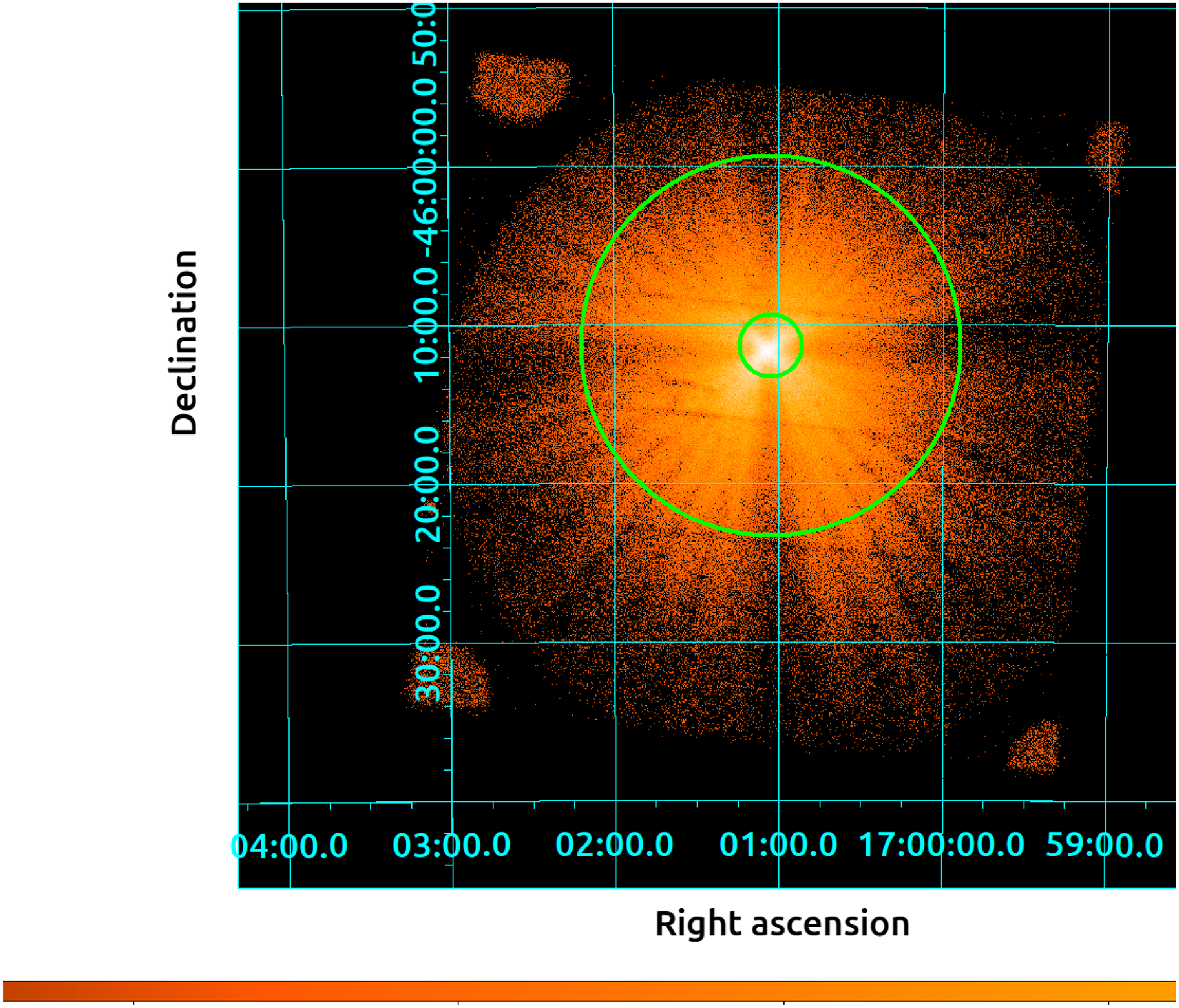
Figure 1. The figure shows the SXT image of the source in the $0.3-8$
keV energy band. The bright spots at the four corners are image of Fe
$0.3-8$
keV energy band. The bright spots at the four corners are image of Fe $^{55}$
calibration sources. The annular region used to extract the lightcurves and spectra is also shown. For details see the text.
$^{55}$
calibration sources. The annular region used to extract the lightcurves and spectra is also shown. For details see the text.
3. Data analysis
3.1 Generation of HID and lightcurve
Since the LAXPC20 unit has a stable gain, we used the events from this unit to create the lightcurve and HID. The task laxpcl1 of LAXPCSOFT package is used to generate the source and background lightcurves as well as spectra. The background level for LAXPC20 in the energy band $3-30$
keV during our observations was
$3-30$
keV during our observations was $\sim$
70-80 counts/s. The time bin size used to extract the lightcurve is 256s. We have combined both Obs A and Obs B while generating the lightcurve. We have plotted the MAXI lightcurve in the energy band
$\sim$
70-80 counts/s. The time bin size used to extract the lightcurve is 256s. We have combined both Obs A and Obs B while generating the lightcurve. We have plotted the MAXI lightcurve in the energy band $2-20$
keV in Figure 2. In Figure 2, the LAXPC lightcurve in the energy band
$2-20$
keV in Figure 2. In Figure 2, the LAXPC lightcurve in the energy band $3-60$
keV and variation in the LAXPC hardness ratio are also shown as inset. Here, the LAXPC hardness ratio is defined as ratio of count rates in the energy bands
$3-60$
keV and variation in the LAXPC hardness ratio are also shown as inset. Here, the LAXPC hardness ratio is defined as ratio of count rates in the energy bands $9.7-20$
keV and 4.6-9.7 keV. The Obs A and Obs B are marked with two vertical lines in the figure. In addition we have also plotted the hardness ratio for the MAXI observations and LAXPC observations. It is clear from the Figure 2 that both AstroSat observations took place close to peak of the outburst. We have also marked the position of dipping FB (FB2) in the inset figure using vertical lines. The hardness ratio for the MAXI observations are defined as ratio of count rates in the energy bands
$9.7-20$
keV and 4.6-9.7 keV. The Obs A and Obs B are marked with two vertical lines in the figure. In addition we have also plotted the hardness ratio for the MAXI observations and LAXPC observations. It is clear from the Figure 2 that both AstroSat observations took place close to peak of the outburst. We have also marked the position of dipping FB (FB2) in the inset figure using vertical lines. The hardness ratio for the MAXI observations are defined as ratio of count rates in the energy bands $10-20$
keV and
$10-20$
keV and $4-10$
keV. The LAXPC20 lightcurves in the energy ranges
$4-10$
keV. The LAXPC20 lightcurves in the energy ranges $6.5-9.7$
keV,
$6.5-9.7$
keV, $9.7-20$
keV, and
$9.7-20$
keV, and $3-20$
keV are used to generate the HID. In the HID ratio of the count rates in the energy bands
$3-20$
keV are used to generate the HID. In the HID ratio of the count rates in the energy bands $9.7-20$
keV and
$9.7-20$
keV and $6.5-9.7$
keV are plotted against intensity in the
$6.5-9.7$
keV are plotted against intensity in the $3-20$
keV energy band. In Figure 3 we show the HID of the source, where each point corresponds to a 256s bin size. HID has an extended HB and a less prominent dipping FB. The different regions of the Z-track are marked with boxes. We extract the spectra and the power-density spectra (PDS) corresponding to these sections to study their evolution along the HID. The HB has been divided in four segments: HB1,HB2, HB3, HB4. The NB has four sections: NB1, NB2, NB3, NB4. The FB is divided in FB1 and FB2. We also created CCD using lightcurves in energy bands
$3-20$
keV energy band. In Figure 3 we show the HID of the source, where each point corresponds to a 256s bin size. HID has an extended HB and a less prominent dipping FB. The different regions of the Z-track are marked with boxes. We extract the spectra and the power-density spectra (PDS) corresponding to these sections to study their evolution along the HID. The HB has been divided in four segments: HB1,HB2, HB3, HB4. The NB has four sections: NB1, NB2, NB3, NB4. The FB is divided in FB1 and FB2. We also created CCD using lightcurves in energy bands $3.0-4.6$
keV,
$3.0-4.6$
keV, $4.6-6.5$
keV,
$4.6-6.5$
keV, $6.5-9.7$
keV and
$6.5-9.7$
keV and $9.7-20$
keV. The soft colors are calculated by taking ratio of the count rate in the energy bands
$9.7-20$
keV. The soft colors are calculated by taking ratio of the count rate in the energy bands $4.6-6.5$
keV and
$4.6-6.5$
keV and $3.0-4.6$
keV and the hard color is computed by taking ratio of the count rate in the energy bands
$3.0-4.6$
keV and the hard color is computed by taking ratio of the count rate in the energy bands $6.5-9.7$
keV and
$6.5-9.7$
keV and $9.7-20$
keV bands. We show the CCD of the source in Figure 4.
$9.7-20$
keV bands. We show the CCD of the source in Figure 4.
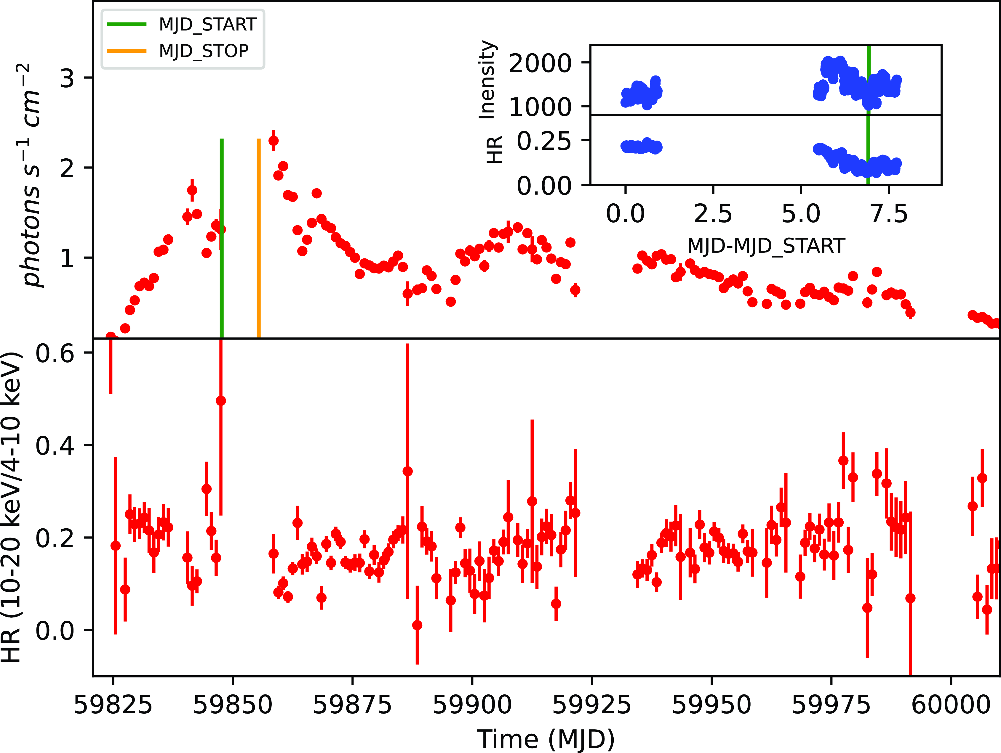
Figure 2. The figure shows the MAXI lightcurve of the source in the energy band $2-20$
keV and hardness ratio calculated using energy band 10-20 keV and 4-10 keV. The two vertical line marks the AstroSat observations. The inset figure in top panel shows the LAXPC lightcurve in
$2-20$
keV and hardness ratio calculated using energy band 10-20 keV and 4-10 keV. The two vertical line marks the AstroSat observations. The inset figure in top panel shows the LAXPC lightcurve in $3-60$
keV energy band and hardness ratio calculated using energy bands 9.7-20 keV and 4.6-9.7 keV. In the inset figure intensity is defined as counts rate in the 3-60 keV energy band. The start and stop time of the dipping FB is marked by two vertical lines in the inset figure. Since the dip period is short (
$3-60$
keV energy band and hardness ratio calculated using energy bands 9.7-20 keV and 4.6-9.7 keV. In the inset figure intensity is defined as counts rate in the 3-60 keV energy band. The start and stop time of the dipping FB is marked by two vertical lines in the inset figure. Since the dip period is short ( $\sim$
3000 seconds) both vertical lines are merged.
$\sim$
3000 seconds) both vertical lines are merged.
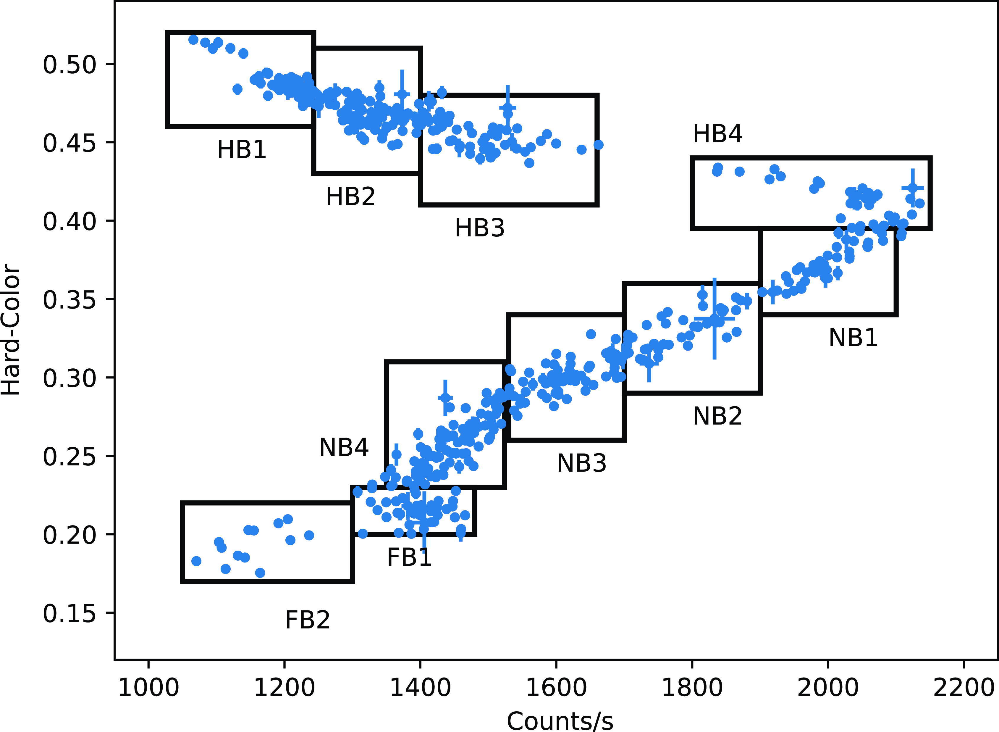
Figure 3. The figure shows the HID of the source. Hard-color is ratio of the count rates in the energy bands $9.7-20$
keV and
$9.7-20$
keV and $6.5-9.7$
keV and intensity is defined as count rate in the energy range
$6.5-9.7$
keV and intensity is defined as count rate in the energy range $3-20$
keV.
$3-20$
keV.
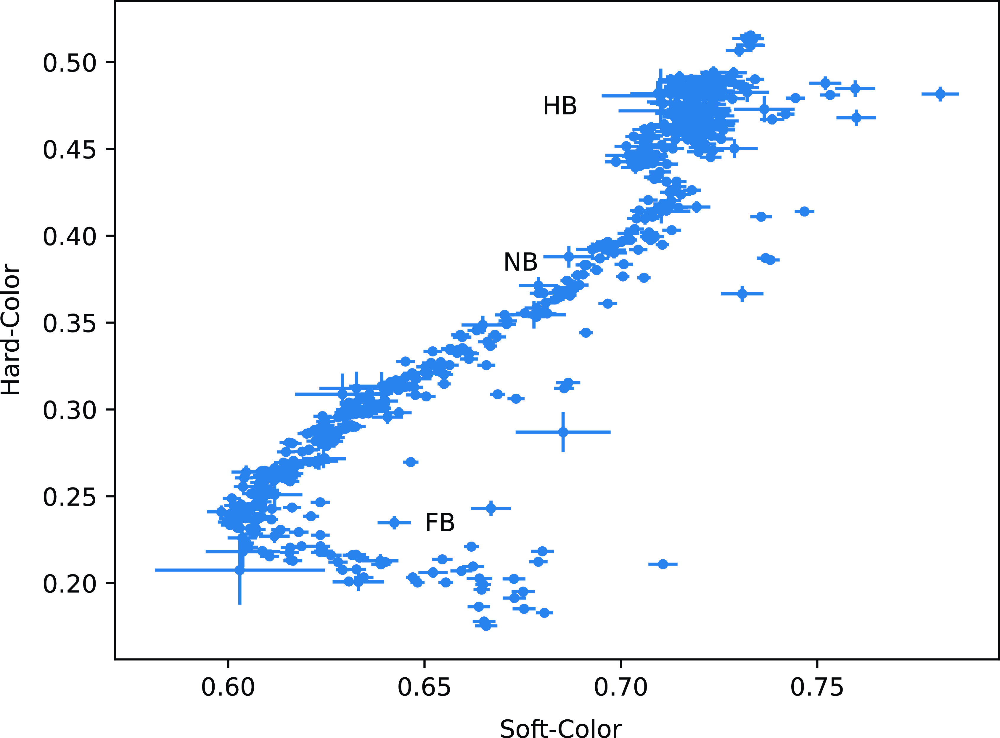
Figure 4. The figure shows the CCD of the source. Hard-color is ratio of the count rates in the energy bands $9.7-20$
keV and
$9.7-20$
keV and $6.5-9.7$
keV and soft color is defined as count rate in the energy range
$6.5-9.7$
keV and soft color is defined as count rate in the energy range $4.6-6.5$
and
$4.6-6.5$
and $3.0-4.6$
keV.
$3.0-4.6$
keV.
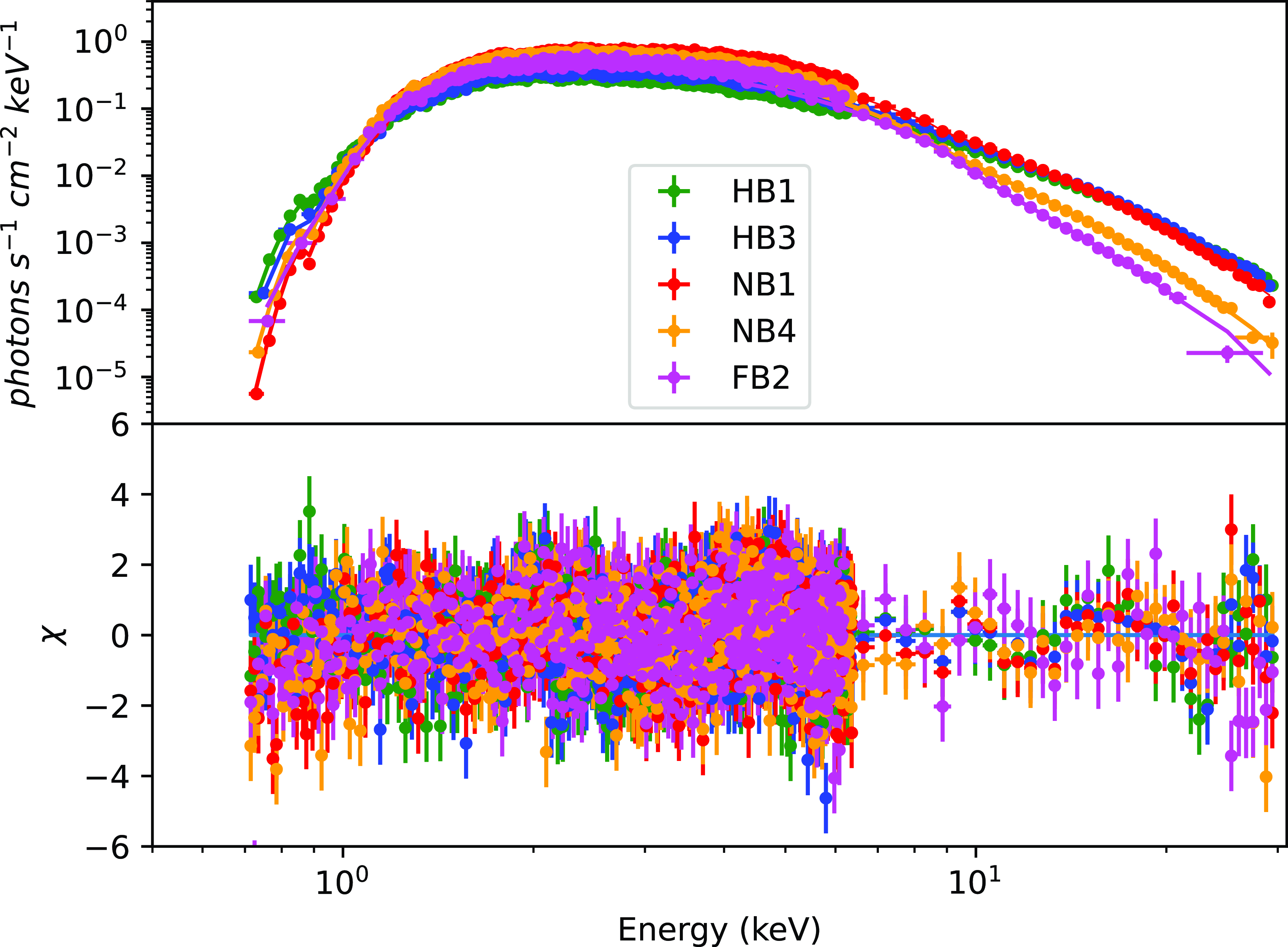
Figure 5. In the top panel of the figure the unfolded spectra and the best-fit model together for the segments HB1,HB3, NB1, NB4 and FB2 have been plotted. The best-fit model used here is tbabs*(diskbb+Comptb). The residual in units of sigma for these segments is also plotted in the bottom panel of the figure.
Table 1. Best-fit parameters obtained by fitting the spectra for all segments of HID using model tbabs*(bbodyrad+diskbb) (Model 1). The fit parameters are $N_H$
in units of
$N_H$
in units of $10^{22} cm^{-2}$
, disk temperature
$10^{22} cm^{-2}$
, disk temperature $kT_{in}$
, disk normalisation
$kT_{in}$
, disk normalisation $N_{MCD}$
, blackbody temperature
$N_{MCD}$
, blackbody temperature $kT_{BB}$
and blackbody normalisation
$kT_{BB}$
and blackbody normalisation $N_{BB}$
. The reduced
$N_{BB}$
. The reduced $\chi^2$
(
$\chi^2$
( $\chi^2/dof)$
is also given in the last column.
$\chi^2/dof)$
is also given in the last column.
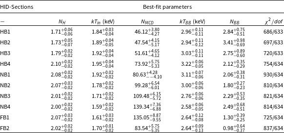
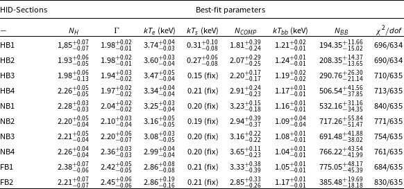
Table 2. Best-fit parameters obtained by fitting the spectra for different segments of HID using model tbabs*(bbodyrad+nthComp) (Model 2). The fit parameters are the hydrogen column density $N_H$
in units of
$N_H$
in units of $10^{22} cm^{-2}$
, the photon index
$10^{22} cm^{-2}$
, the photon index $\Gamma$
, the electron temperature
$\Gamma$
, the electron temperature $kT_e$
, the seed photon temperature
$kT_e$
, the seed photon temperature $kT_s$
and normalisation of the Comptonised component
$kT_s$
and normalisation of the Comptonised component $N_{COMP}$
the blackbody temperature
$N_{COMP}$
the blackbody temperature $kT_{BB}$
and the blackbody normalisation
$kT_{BB}$
and the blackbody normalisation $N_{BB}$
. The reduced
$N_{BB}$
. The reduced $\chi^2$
(
$\chi^2$
( $\chi^2/dof$
) is also presented in the last column of the table.
$\chi^2/dof$
) is also presented in the last column of the table.
3.2 Analysis of spectroscopic data
X-ray spectra using the LAXPC20 data and the SXT data were extracted for all the ten segments of the HID. These spectra were modeled and analysed using XSPEC version 12.13. We consider the LAXPC20 data up to 30 keV for the spectral fitting due to limited statistics above 30 keV and dominance of the background at higher energies. The SXT data in the energy range $0.7-7$
keV are used for the combined spectral fitting. The combined broad band spectra in the energy band
$0.7-7$
keV are used for the combined spectral fitting. The combined broad band spectra in the energy band $0.7-30$
keV are fitted with the three different approaches. First we used the combination of a MCD (diskbb in XSPEC) and a simple blackbody (BB) emission (bbodyrad in XSPEC). The model MCD+BB (hereafter Model 1) has been used previously to model the spectra of this source (Lin, Remillard, and Homan, 2009) and emission in the soft state of two atoll sources (Lin, Remillard, and Homan, 2007). We also added a constrained broken power-law (CBPL) component to the Model 1 following Lin, Remillard, and Homan (2009). The photon index (
$0.7-30$
keV are fitted with the three different approaches. First we used the combination of a MCD (diskbb in XSPEC) and a simple blackbody (BB) emission (bbodyrad in XSPEC). The model MCD+BB (hereafter Model 1) has been used previously to model the spectra of this source (Lin, Remillard, and Homan, 2009) and emission in the soft state of two atoll sources (Lin, Remillard, and Homan, 2007). We also added a constrained broken power-law (CBPL) component to the Model 1 following Lin, Remillard, and Homan (2009). The photon index ( $\Gamma_1$
) was frozen to a value 2.5 and break energy (
$\Gamma_1$
) was frozen to a value 2.5 and break energy ( $E_{break}$
) was fixed at 20 keV. The second power-law index was frozen to the best fit values. Only normalisation of CBPL was left free. The model improves the fit for HB1, HB2 and HB3. However, for other sections of the Z-track addition of this component did not improve the fit. Hence CBPL was not added in Model 1 for these sections.
$E_{break}$
) was fixed at 20 keV. The second power-law index was frozen to the best fit values. Only normalisation of CBPL was left free. The model improves the fit for HB1, HB2 and HB3. However, for other sections of the Z-track addition of this component did not improve the fit. Hence CBPL was not added in Model 1 for these sections.
We also tried BB plus a Comptonised emission (hereafter Model 2). We used the nthComp component in XSPEC (see Zdziarski, Johnson, and Magdziarz Reference Zdziarski, Johnson and Magdziarz1996 for details) to describe the Comptonised emission. Finally, we attempted a combination of MCD and nthComp (hereafter Model 3) components to describe the X-ray spectra of this source. Both models have been widely used to fit the spectra of the NS-LMXBs (Di Salvo et al., Reference Di Salvo, Robba, Iaria, Stella, Burderi and Israel2001; Barret, Reference Barret2001; Di Salvo et al., Reference Di Salvo, Robba, Iaria, Stella, Burderi and Israel2001; Agrawal and Sreekumar, Reference Agrawal and Sreekumar2003; Agrawal, Nandi, and Katoch, Reference Agrawal, Nandi and Katoch2023). We also need an additional smeared edge component (at $\sim$ $7-8$
keV) to improve the fit. Model 2 does not require this additional smeared edge component. TBabs model (Wilms, Allen, and McCray, Reference Wilms, Allen and McCray2000) is used to take into account the absorption of X-rays in the inter stellar medium. We added 2 per cent systematic error while carrying out the joint spectral fitting of the LAXPC20 and SXT spectra in XSPEC to account for uncertainty in the response matrices of both detectors. We also added a multiplicative constant component to account for the cross calibration related uncertainties. We take shape of the seed photon spectrum as blackbody while fitting the data with Model 3 and diskbb for Model 2.
$7-8$
keV) to improve the fit. Model 2 does not require this additional smeared edge component. TBabs model (Wilms, Allen, and McCray, Reference Wilms, Allen and McCray2000) is used to take into account the absorption of X-rays in the inter stellar medium. We added 2 per cent systematic error while carrying out the joint spectral fitting of the LAXPC20 and SXT spectra in XSPEC to account for uncertainty in the response matrices of both detectors. We also added a multiplicative constant component to account for the cross calibration related uncertainties. We take shape of the seed photon spectrum as blackbody while fitting the data with Model 3 and diskbb for Model 2.
We also attempt to fit the data with Comptb model, which takes care of both thermal and bulk Comptonisation (Farinelli et al., Reference Farinelli, Titarchuk, Paizis and Frontera2008). This models is sum of two components, the soft seed photons which has not undergone up-scattering and coming directly and the component that is Comptonised. We fix $\gamma$
= 3 (blackbody seed photon). We find that parameter
$\gamma$
= 3 (blackbody seed photon). We find that parameter $\log A$
pegs to 8 and
$\log A$
pegs to 8 and $\delta$ $\lt\lt1$
. Since seed photons from disc can also be Comptonised by the Corona, we included one more Comptb component and tied the value of spectral index
$\lt\lt1$
. Since seed photons from disc can also be Comptonised by the Corona, we included one more Comptb component and tied the value of spectral index $\alpha$
and electron temperature
$\alpha$
and electron temperature $kT_e$
while fitting the data with double Comptb. For the second Comptb component
$kT_e$
while fitting the data with double Comptb. For the second Comptb component $\log A$
pegs to -8 and
$\log A$
pegs to -8 and $\delta \lt\lt1$
. For the first Comptb component, illumination factor (
$\delta \lt\lt1$
. For the first Comptb component, illumination factor ( $A/(A+1)$
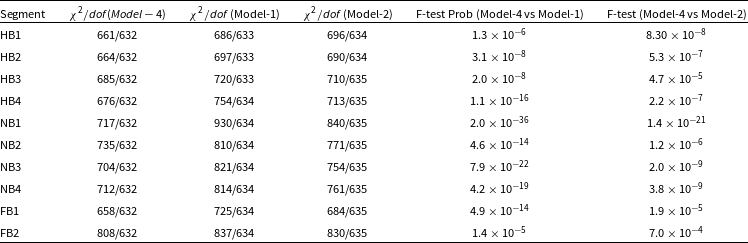
) is close to one and for the second Comptb component it is negligible. Hence, we reached to conclusion that the bulk Comptonisation is not present, disk photons are seen directly and blackbody photons from the NS surface is completely Comptonised. Hence, we fit the data with Comptb plus diskbb component (Model 4) which allow us to calculate the inner disk radius as well. We have shown the unfolded spectra using Model 4 for the segments, HB1, HB3, NB1, NB4 and FB2 for a comparison in Figure 5. We compared Model-4, with Model-1 and Model-2 by computing F-test chance improvement probabilities for addition of extra parameters. Model 3 and Model 4 has similar reduced
$A/(A+1)$
) is close to one and for the second Comptb component it is negligible. Hence, we reached to conclusion that the bulk Comptonisation is not present, disk photons are seen directly and blackbody photons from the NS surface is completely Comptonised. Hence, we fit the data with Comptb plus diskbb component (Model 4) which allow us to calculate the inner disk radius as well. We have shown the unfolded spectra using Model 4 for the segments, HB1, HB3, NB1, NB4 and FB2 for a comparison in Figure 5. We compared Model-4, with Model-1 and Model-2 by computing F-test chance improvement probabilities for addition of extra parameters. Model 3 and Model 4 has similar reduced $\chi^2$
. Model 4 provides statistically better fit compared to Model 1 and Model 2 (see Table 6). We also note that Model 2 does not constrain the seed photon temperature in the segments HB3-FB2. The cflux command is used to derive the unabsorbed fluxes in the individual spectral components. The disk and Comptonisation fluxes are computed in the energy range
$\chi^2$
. Model 4 provides statistically better fit compared to Model 1 and Model 2 (see Table 6). We also note that Model 2 does not constrain the seed photon temperature in the segments HB3-FB2. The cflux command is used to derive the unabsorbed fluxes in the individual spectral components. The disk and Comptonisation fluxes are computed in the energy range $0.5-50.0$
keV. Errors quoted in the best fit parameters are
$0.5-50.0$
keV. Errors quoted in the best fit parameters are $1-\sigma$
errors and computed using
$1-\sigma$
errors and computed using $\Delta \chi^2=1$
.
$\Delta \chi^2=1$
.
3.3 Timing analysis
We carry out fast timing analysis using the LAXPC20 data. Using the LAXPC20 data, we generated 2-ms binned lightcurves in the energy band $3-50$
keV for each data points (with 256s length) of HID. We divided these lightcurves in intervals of 4096 bins and created the PDS for these intervals. This procedure produces PDS in the frequency range
$3-50$
keV for each data points (with 256s length) of HID. We divided these lightcurves in intervals of 4096 bins and created the PDS for these intervals. This procedure produces PDS in the frequency range $0.12-250$
Hz for each intervals. PDS belonging to same segments of the HID were averaged and re-binned geometrically by a factor of 1.03 in the frequency space. The PDS were normalised to give fractional root-mean squared power
$0.12-250$
Hz for each intervals. PDS belonging to same segments of the HID were averaged and re-binned geometrically by a factor of 1.03 in the frequency space. The PDS were normalised to give fractional root-mean squared power $((rms/mean)^2/Hz)$
and dead time corrected Poisson noise was subtracted (Zhang et al., Reference Zhang, Jahoda, Swank, Morgan and Giles1995; Agrawal, Nandi and Ramadevi, 2018). We performed the fitting of PDS in the frequency range
$((rms/mean)^2/Hz)$
and dead time corrected Poisson noise was subtracted (Zhang et al., Reference Zhang, Jahoda, Swank, Morgan and Giles1995; Agrawal, Nandi and Ramadevi, 2018). We performed the fitting of PDS in the frequency range $0.12-250$
Hz using the combination of Lorentzian and power-law components. The Lorentzian function is defined as
$0.12-250$
Hz using the combination of Lorentzian and power-law components. The Lorentzian function is defined as
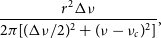 \begin{equation} \frac{r^2 \Delta \nu} {2\pi [(\Delta\nu/2)^2+(\nu-\nu_c)^2]}, \end{equation}
where $\Delta \nu$
is the full-width at half maxima (FWHM),
$\Delta \nu$
is the full-width at half maxima (FWHM), $\nu_c$
is the centroid frequency and r is the integrated rms for the Lorentzian component (Belloni, Psaltis, and van der Klis, Reference Belloni, Psaltis and van der Klis2002). 1-
$\nu_c$
is the centroid frequency and r is the integrated rms for the Lorentzian component (Belloni, Psaltis, and van der Klis, Reference Belloni, Psaltis and van der Klis2002). 1- $\sigma$
errors (68% confidence) in the best-fit parameters are calculated using
$\sigma$
errors (68% confidence) in the best-fit parameters are calculated using $\Delta \chi^2=1$
. We also created PDS in the energy bands
$\Delta \chi^2=1$
. We also created PDS in the energy bands $3-5$
keV,
$3-5$
keV, $5-8$
keV, and
$5-8$
keV, and $8-15$
keV to carry out the energy dependent study of the observed power-spectral features.
$8-15$
keV to carry out the energy dependent study of the observed power-spectral features.
Table 3. Best-fit parameters obtained by fitting the spectra of different sections of the Z-track using model tbabs(nthComp+diskbb) (Model 3). The parameters of the fits are $N_H$
in units of
$N_H$
in units of $10^{22} cm^{-2}$
, photon index
$10^{22} cm^{-2}$
, photon index $\Gamma$
, electron temperature
$\Gamma$
, electron temperature $ kT_e$
, disk temperature
$ kT_e$
, disk temperature $kT_{in}$
, normalisation of Comptonised component
$kT_{in}$
, normalisation of Comptonised component $N_{comp}$
, seed photon temperature
$N_{comp}$
, seed photon temperature $kT_{s}$
, disk normalisation
$kT_{s}$
, disk normalisation $N_{MCD}$
.
$N_{MCD}$
.
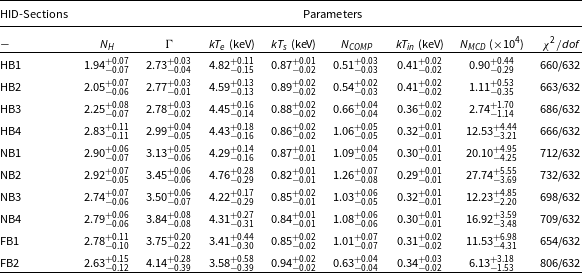
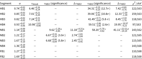
Table 4. Best-fit parameters obtained by fitting the spectra of different sections of the Z-track using model tbabs(Comptb+diskbb) (Model 4). The parameters of the fits are $N_H$
in units of
$N_H$
in units of $10^{22} cm^{-2}$
, energy index
$10^{22} cm^{-2}$
, energy index $\alpha$
, electron temperature
$\alpha$
, electron temperature $ kT_e$
, disk temperature
$ kT_e$
, disk temperature $kT_{in}$
, normalisation of Comptonised component
$kT_{in}$
, normalisation of Comptonised component $N_{comp}$
, seed photon temperature
$N_{comp}$
, seed photon temperature $kT_{s}$
, disk normalisation
$kT_{s}$
, disk normalisation $N_{MCD}$
.
$N_{MCD}$
.
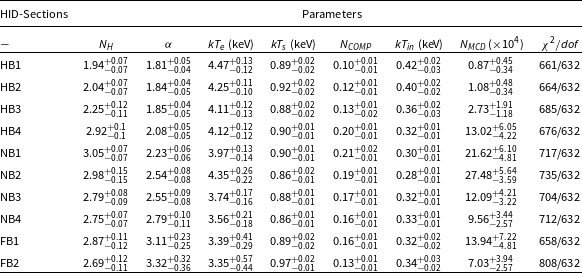
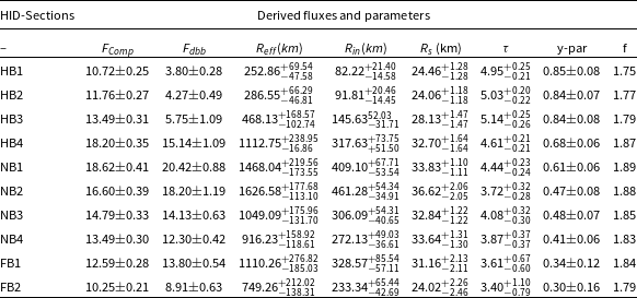
Table 5. The table provides the Comptonisation flux $F_{Comp}$
and disk flux
$F_{Comp}$
and disk flux $F_{dbb}$
in the energy range
$F_{dbb}$
in the energy range $0.5-50.0$
keV. All the fluxes are in units of
$0.5-50.0$
keV. All the fluxes are in units of $10^{-9}$
ergs/s/cm
$10^{-9}$
ergs/s/cm $^2$
. The disk radius
$^2$
. The disk radius $R_{eff}$
, seed photon radius
$R_{eff}$
, seed photon radius $R_s$
, optical depth
$R_s$
, optical depth $\tau$
and color correction factor are also given. See text for details. The derived values are for the Model 4
$\tau$
and color correction factor are also given. See text for details. The derived values are for the Model 4
4. Results
4.1 Spectral nature of XTE J1701-462
In Figure 3, we show the HID of the source. The HID has an extended HB and short and dipping FB. Figure 4 shows the CCD of the source. The points belonging to the HB on the CCD are clustered. The source traced similar pattern on the CCD and HID during the Cyg-like phase of 2007 outburst (Homan et al., Reference Homan, van der Klis, Wijnands, Belloni, Fender, Klein-Wolt and Casella2007). We fit the broad band X-ray spectra corresponding to different segments of the HID of the source using various popular spectral models and study evolution of the parameters along the Z-track. We note that both Model 4 and Model 3 comprising disk-blackbody and Comptonised emission are statistically better description of the data. The seed photon energy cannot be constrained for sections HB3 to FB2, while using Model 2. It is also noted that the high blackbody temperature ( $\sim$
3 keV) obtained by fitting the broad band spectra with Model 1 seems to be unphysical. In Figure 5 we show the unfolded X-ray spectra for different sections fitted with Model 4. The best-fit parameters obtained using Model 1, Model 2,Model 3 and Model 4 are listed in Tables 1, 2, 3 and 4 respectively. The unabsorbed disk and Comptonised component fluxes are listed Table 5. The model component diskbb has two parameters, the inner disk temperature
$\sim$
3 keV) obtained by fitting the broad band spectra with Model 1 seems to be unphysical. In Figure 5 we show the unfolded X-ray spectra for different sections fitted with Model 4. The best-fit parameters obtained using Model 1, Model 2,Model 3 and Model 4 are listed in Tables 1, 2, 3 and 4 respectively. The unabsorbed disk and Comptonised component fluxes are listed Table 5. The model component diskbb has two parameters, the inner disk temperature $kT_{in}$
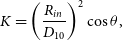
and the normalisation K. The normalisation K is connected with the inner disk radius
$kT_{in}$
and the normalisation K. The normalisation K is connected with the inner disk radius $R_{in}$
by the relation,
$R_{in}$
by the relation,
 \begin{equation} K=\left(\frac{R_{in}}{D_{10}}\right)^2\cos\theta, \end{equation}
where $D_{10}$
is the distance in units of 10 kpc and
$D_{10}$
is the distance in units of 10 kpc and $\theta$
is inclination angle of the disk (Mitsuda et al., Reference Mitsuda, Inoue, Koyama, Makishima, Matsuoka, Ogawara, Shibazaki, Suzuki, Tanaka and Hirano1984). We assumed distance of the source to be 8.8 kpc and inclination angle to be 60
$\theta$
is inclination angle of the disk (Mitsuda et al., Reference Mitsuda, Inoue, Koyama, Makishima, Matsuoka, Ogawara, Shibazaki, Suzuki, Tanaka and Hirano1984). We assumed distance of the source to be 8.8 kpc and inclination angle to be 60 $^\circ$
(Lin et al., Reference Lin, Altamirano, Homan, Remillard, Wijnands and Belloni2009; Lin, Remillard, and Homan, 2009). The absence of iron line (as in the present case) or presence of weak iron line and absence of X-ray dips and eclipses suggests that inclination should be less than 70
$^\circ$
(Lin et al., Reference Lin, Altamirano, Homan, Remillard, Wijnands and Belloni2009; Lin, Remillard, and Homan, 2009). The absence of iron line (as in the present case) or presence of weak iron line and absence of X-ray dips and eclipses suggests that inclination should be less than 70 $^\circ$
. Hence, we chose an average inclination angle of 60
$^\circ$
. Hence, we chose an average inclination angle of 60 $^\circ$
to compute the inner disk radius. The local blackbody spectrum from the accretion disc is modified by scattering processes and can be best represented by a diluted blackbody (Shimura and Takahara, Reference Shimura and Takahara1995) given by equation
$^\circ$
to compute the inner disk radius. The local blackbody spectrum from the accretion disc is modified by scattering processes and can be best represented by a diluted blackbody (Shimura and Takahara, Reference Shimura and Takahara1995) given by equation
 \begin{equation} F^{db}_\nu = \frac{1}{f^4} \pi B_\nu(fT_{eff}), \end{equation}
where f is spectral hardening factor, $T_{eff}$
is effective temperature. The effective temperature is given by
$T_{eff}$
is effective temperature. The effective temperature is given by $T_{eff} = \frac{T_{in}}{f}$
and effective inner accretion on disc radius is given by
$T_{eff} = \frac{T_{in}}{f}$
and effective inner accretion on disc radius is given by $R_{eff} = f^2 R_{in}$
. We computed the color correction factor f using the equation (Davis and El-Abd, Reference Davis and El-Abd2019)
$R_{eff} = f^2 R_{in}$
. We computed the color correction factor f using the equation (Davis and El-Abd, Reference Davis and El-Abd2019)
 \begin{align} f \approx 1.48 &+ 0.33(\log \dot{m} +1) + 0.07 (\log \alpha+1) \nonumber\\&+ 0.02 (\log(M/M_\odot) -1), \end{align}
here $\dot{m}$
is the mass accretion rate in unit of Eddington rate,
$\dot{m}$
is the mass accretion rate in unit of Eddington rate, $\alpha$
is the viscosity parameter and M is the mass of neutron star. Color factors are listed in Table 5.
$\alpha$
is the viscosity parameter and M is the mass of neutron star. Color factors are listed in Table 5. $R_{eff}$
was derived using these values and given in the Table 5. The Comptb component has four free parameters, the spectral index
$R_{eff}$
was derived using these values and given in the Table 5. The Comptb component has four free parameters, the spectral index $\alpha$
, the electron temperature
$\alpha$
, the electron temperature $kT_e$
of the hot corona, the seed photon energy
$kT_e$
of the hot corona, the seed photon energy $kT_s$
, and the normalisation. The radius of seed photon emitting region is given by the equation (see in ’t Zand et al. Reference in ’t Zand, Verbunt, Strohmayer, Bazzano, Cocchi, Heise and van Kerkwijk1999),
$kT_s$
, and the normalisation. The radius of seed photon emitting region is given by the equation (see in ’t Zand et al. Reference in ’t Zand, Verbunt, Strohmayer, Bazzano, Cocchi, Heise and van Kerkwijk1999),
 \begin{equation}R_s = 3 \times 10^4 \sqrt{F_{comp}/(1+y)}/(kT_s)^2\end{equation}
Table 6. Fit-statistics to compare 3 different models used to describe the X-ray spectra of the source. We have compared Model-3 with Model-1 and Model-2 by computing F-test chance improvement probabilities
The above equation is obtained by equating the soft seed photon luminosity with blackbody luminosity of temperature $kT_s$
where is y is the Compton y-parameter that gives relative energy gain due to Compton scattering and is given by the relation
$kT_s$
where is y is the Compton y-parameter that gives relative energy gain due to Compton scattering and is given by the relation
 \begin{equation} y=\frac{4kT_e}{m_e c^2} \tau^2,\end{equation}
where $\tau$
is the optical depth.
$\tau$
is the optical depth.
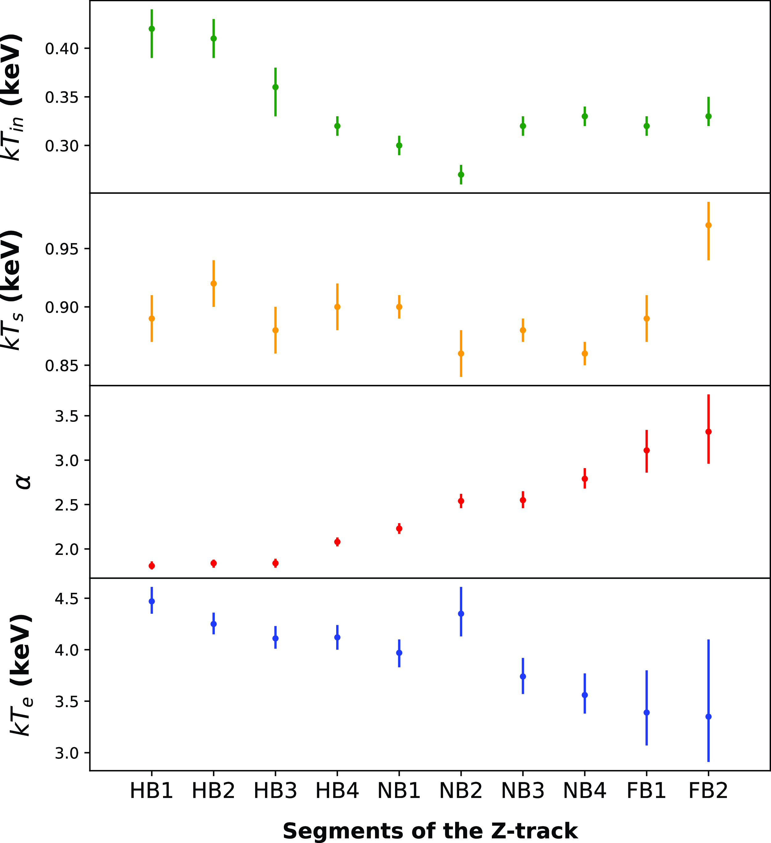
Figure 6. Figure shows evolution of the parameters of Model 4 (tbabs*(Comptb+diskbb)). The electron temperature $kT_e$
and spectral index
$kT_e$
and spectral index $\alpha$
show significant evolution as the source moves from HB to FB. The Comptonised component becomes softer from segment HB1 to FB2. Also disk temperature decreases as the source moves from the segment HB1 to NB2. For details see the text and Table 4.
$\alpha$
show significant evolution as the source moves from HB to FB. The Comptonised component becomes softer from segment HB1 to FB2. Also disk temperature decreases as the source moves from the segment HB1 to NB2. For details see the text and Table 4.
The spectral index of Comptonised component is given by (see Zdziarski, Johnson, and Magdziarz Reference Zdziarski, Johnson and Magdziarz1996)
 \begin{equation}\alpha = \left[\frac{9}{4}+\frac{1}{kT_e/m_e c^2(1+\tau/3)}\right]^{1/2}-\frac{3}{2}\end{equation}
We solve this relation for optical depth $\tau$
. The optical depth depends upon
$\tau$
. The optical depth depends upon $\alpha$
and electron temperature
$\alpha$
and electron temperature $kT_e$
. We show the variation of the fitted (see Figure 6) and derived parameters (Figure 7) of Model 4 as a function of position on the HID. An increase in the
$kT_e$
. We show the variation of the fitted (see Figure 6) and derived parameters (Figure 7) of Model 4 as a function of position on the HID. An increase in the $\alpha$
from
$\alpha$
from $\sim$
1.81 to 3.32 is observed with the movement of the source from the HB to the NB then to the FB, suggesting that the Comptonised spectrum is becoming softer. The electron temperature
$\sim$
1.81 to 3.32 is observed with the movement of the source from the HB to the NB then to the FB, suggesting that the Comptonised spectrum is becoming softer. The electron temperature $kT_e$
of the Compton corona also decreases from 4.48 to 3.35 as the source moves along the Z-track from HB to FB. The seed photon temperature remains almost constant and remains in the narrow range
$kT_e$
of the Compton corona also decreases from 4.48 to 3.35 as the source moves along the Z-track from HB to FB. The seed photon temperature remains almost constant and remains in the narrow range $0.9-1.0$
keV. The disk temperature
$0.9-1.0$
keV. The disk temperature $kT_{in}$
decreases from
$kT_{in}$
decreases from $\sim$
0.42 to
$\sim$
0.42 to $\sim$
0.28 keV from the segment HB1 to NB2 and then remains almost unchanged in the rest of the Z-track. Our analysis also reveals that the flux of the Comptonised emission in the energy range
$\sim$
0.28 keV from the segment HB1 to NB2 and then remains almost unchanged in the rest of the Z-track. Our analysis also reveals that the flux of the Comptonised emission in the energy range $0.5-50$
keV increases from HB1 to NB1 and then decreases from NB1 to FB2. The disk flux also show a variation similar to the Comptonised flux as the source moves along the HID. We also note that the inner disk radius
$0.5-50$
keV increases from HB1 to NB1 and then decreases from NB1 to FB2. The disk flux also show a variation similar to the Comptonised flux as the source moves along the HID. We also note that the inner disk radius $R_{eff}$
changes from
$R_{eff}$
changes from $\sim$
250 km to
$\sim$
250 km to $\sim$
1600 km as as the source evolves from the state HB1 to NB2 and as it moves further from NB3 to FB2 the disk radius decrease to
$\sim$
1600 km as as the source evolves from the state HB1 to NB2 and as it moves further from NB3 to FB2 the disk radius decrease to $\sim$
750 km. The seed photon radius
$\sim$
750 km. The seed photon radius $R_s$
is found to be in the range of
$R_s$
is found to be in the range of $\sim$ $25 - 36$
km being lowest in the upper HB (HB1 and HB2). The optical depth
$25 - 36$
km being lowest in the upper HB (HB1 and HB2). The optical depth $\tau$
of the corona is slightly higher (
$\tau$
of the corona is slightly higher ( $\tau \sim 4.6-5.1)$
in the HB compared to that in NB and FB. A decrease in
$\tau \sim 4.6-5.1)$
in the HB compared to that in NB and FB. A decrease in $\tau$
from
$\tau$
from $\sim$
4.6 to
$\sim$
4.6 to $\sim$
3.4 is seen with the motion of the source from HB4 to FB2. The
$\sim$
3.4 is seen with the motion of the source from HB4 to FB2. The $y-par$
remains almost constant in HB and then decreases along the NB and FB (see Table 5).
$y-par$
remains almost constant in HB and then decreases along the NB and FB (see Table 5).
4.2 Timing behaviour of XTE J1701-462
To describe the features in the PDS, we need Lorentzian and power-law (Power $\propto \nu^{-\alpha}$
) components. The power-law function describes the very low-frequency noise (VLFN). A zero centred Lorentzian describes the band limited noise (BLN). The narrow features observed in the PDS are also represented by a Lorentzian. Following Belloni, Psaltis, and van der Klis (Reference Belloni, Psaltis and van der Klis2002), we define the characteristic frequency of the narrow features (QPO) as,
$\propto \nu^{-\alpha}$
) components. The power-law function describes the very low-frequency noise (VLFN). A zero centred Lorentzian describes the band limited noise (BLN). The narrow features observed in the PDS are also represented by a Lorentzian. Following Belloni, Psaltis, and van der Klis (Reference Belloni, Psaltis and van der Klis2002), we define the characteristic frequency of the narrow features (QPO) as,
 \begin{equation} \nu_{char} = \sqrt{(\Delta\nu/2)^2+\nu_c^2},\end{equation}
where $\nu_c$
and
$\nu_c$
and $\Delta\nu$
are centroid frequency and FWHM (see Equation 1). The break frequency of BLN component is given by
$\Delta\nu$
are centroid frequency and FWHM (see Equation 1). The break frequency of BLN component is given by $\Delta \nu/2$
, where
$\Delta \nu/2$
, where $\Delta \nu$
is the FWHM of the zero centred Lorentzian component. The quality factor (Q) of the QPO is defined as
$\Delta \nu$
is the FWHM of the zero centred Lorentzian component. The quality factor (Q) of the QPO is defined as $\nu_{c}/\Delta \nu$
. The best-fit parameters of power-spectral features are listed in the Table 7 and their rms values are given in Table 8. We detect narrow QPOs (HBOs) with
$\nu_{c}/\Delta \nu$
. The best-fit parameters of power-spectral features are listed in the Table 7 and their rms values are given in Table 8. We detect narrow QPOs (HBOs) with $\nu_{char}$
(or
$\nu_{char}$
(or $\nu_{HBO}$
) in the range
$\nu_{HBO}$
) in the range $34-40$
Hz in the HID segments HB1, HB2 and HB3 (see Figure 8 and Table 7). The significance of HBOs are 12.7
$34-40$
Hz in the HID segments HB1, HB2 and HB3 (see Figure 8 and Table 7). The significance of HBOs are 12.7 $\sigma$
, 10.8
$\sigma$
, 10.8 $\sigma$
, and 5.8
$\sigma$
, and 5.8 $\sigma$
for segments HB1, HB2 and HB3 respectively. We also detect a weak HBO-like feature in HB4 with significance 2.6
$\sigma$
for segments HB1, HB2 and HB3 respectively. We also detect a weak HBO-like feature in HB4 with significance 2.6 $\sigma$
. The significance of QPOs is computed by taking ratio of the normalisation of the Lorentzian and 1-sigma negative error on normalisation (see Sreehari et al. (Reference Sreehari, Nandi, Das, Agrawal, Mandal, Ramadevi and Katoch2020); Majumder et al. (Reference Majumder, Sreehari, Aftab, Katoch, Das and Nandi2022)). BLN feature with break frequency varying from
$\sigma$
. The significance of QPOs is computed by taking ratio of the normalisation of the Lorentzian and 1-sigma negative error on normalisation (see Sreehari et al. (Reference Sreehari, Nandi, Das, Agrawal, Mandal, Ramadevi and Katoch2020); Majumder et al. (Reference Majumder, Sreehari, Aftab, Katoch, Das and Nandi2022)). BLN feature with break frequency varying from $\sim$
6.5 Hz to
$\sim$
6.5 Hz to $\sim$
11 Hz is seen in this region of HB (HB1-HB4). The frequency
$\sim$
11 Hz is seen in this region of HB (HB1-HB4). The frequency $\nu_{HBO}$
and
$\nu_{HBO}$
and $\nu_{break}$
increases as the source travels from HB1 to HB4. This suggest that the frequency of both components are correlated. NBOs with
$\nu_{break}$
increases as the source travels from HB1 to HB4. This suggest that the frequency of both components are correlated. NBOs with $\nu_{char}$
(or
$\nu_{char}$
(or $\nu_{NBO})$ $\sim$
6.7 Hz with rms
$\sim$
6.7 Hz with rms $\sim$
1.7% is observed in the HID section NB2 and NB3 (see Figure 8). The significance of NBOs is given in the Table 7. The rms of the HBOs decreases from
$\sim$
1.7% is observed in the HID section NB2 and NB3 (see Figure 8). The significance of NBOs is given in the Table 7. The rms of the HBOs decreases from $\sim$
4.5% to
$\sim$
4.5% to $\sim$
2.8% as the source travels from HB1 to HB3. The rms of the BLN feature also shows a decrease from
$\sim$
2.8% as the source travels from HB1 to HB3. The rms of the BLN feature also shows a decrease from $\sim$
8.5% to
$\sim$
8.5% to $\sim$
5.2% from HB1 to HB4. The total rms in the PDS decreases as the source moves along the HID from HB1 to FB2. We also find a broad high frequency feature with a quality factor
$\sim$
5.2% from HB1 to HB4. The total rms in the PDS decreases as the source moves along the HID from HB1 to FB2. We also find a broad high frequency feature with a quality factor $\lt2$
with
$\lt2$
with $\nu_{c}$ $\sim$
59 Hz in NB1. Since quality factor of this feature is small, we do not consider it as HBO. We also detect a low-frequency noise (LFN) with
$\sim$
59 Hz in NB1. Since quality factor of this feature is small, we do not consider it as HBO. We also detect a low-frequency noise (LFN) with $\nu_{char}$ $\sim$
9.6 Hz in this section of NB.
$\sim$
9.6 Hz in this section of NB.
We have also carried out energy dependent study of the power-spectral features (see Table 9 for details). The strength of the HBOs increases with increase in the energy of X-ray photons. This trend is observed in the HID sections HB1, HB2 and HB3. However, PDS created in the narrow energy ranges $3-5$
keV,
$3-5$
keV, $5-8$
keV and
$5-8$
keV and $8-15$
keV do not show a significant HBO for the HID segment HB4. Moreover, the rms of BLN feature also show increasing pattern with an increase in the energy. In HB3, HBO was found to be absent in the energy range
$8-15$
keV do not show a significant HBO for the HID segment HB4. Moreover, the rms of BLN feature also show increasing pattern with an increase in the energy. In HB3, HBO was found to be absent in the energy range $3-5$
keV and we set an upper limit of
$3-5$
keV and we set an upper limit of $\lt1.97$
% on the rms of this feature.
$\lt1.97$
% on the rms of this feature.
Table 7. Parameter values obtained by fitting the PDS of different segments of the Z-track. Lorentzian components and power-law are required to describe the BLN, narrow QPOs and VLFN in the PDS. The parameters of the fit are, power-law index $\alpha$
, break frequency
$\alpha$
, break frequency $\nu_{break}$
, the characteristics frequency of the QPOs
$\nu_{break}$
, the characteristics frequency of the QPOs $\nu_{char}$
(
$\nu_{char}$
( $\nu_{HBO}$
for HBO and
$\nu_{HBO}$
for HBO and $\nu_{NBO}$
for NBO) and full-width half-maxima
$\nu_{NBO}$
for NBO) and full-width half-maxima $\Delta \nu $
.
$\Delta \nu $
.
a The frequency of LFN
b FWHM of LFN
c Frequency of HFN
d FWHM of HFN
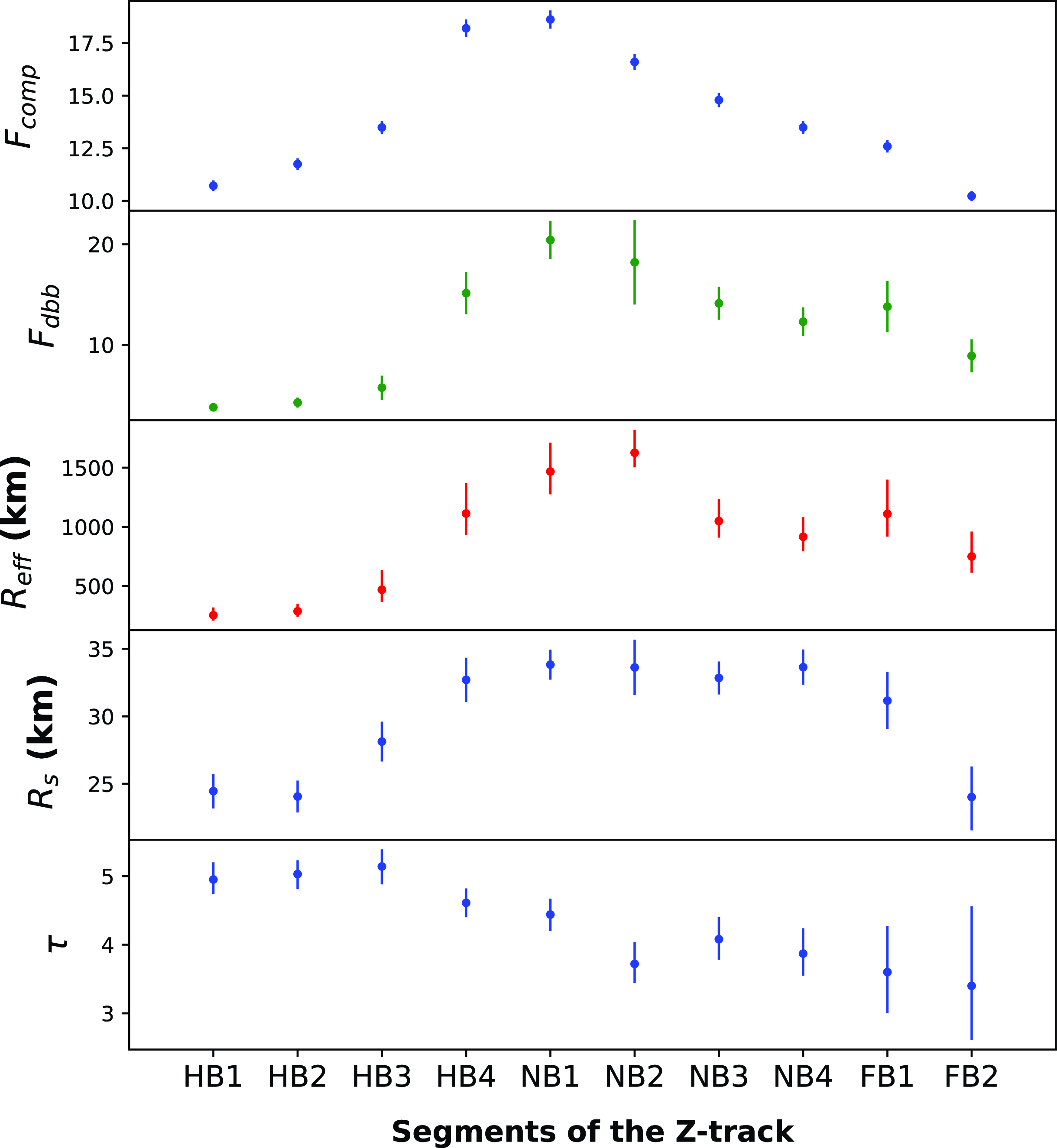
Figure 7. Figure shows evolution of the Comptonised ( $F_{Comp})$
flux, disk flux (
$F_{Comp})$
flux, disk flux ( $F_{dbb})$
, the effective inner disk radius (
$F_{dbb})$
, the effective inner disk radius ( $R_{eff}$
) and the optical depth (
$R_{eff}$
) and the optical depth ( $\tau$
) of the corona, calculated for Model 4. Significant evolution of the disk and the Comptonised flux is clearly visible. The effective disk radius and optical depth (
$\tau$
) of the corona, calculated for Model 4. Significant evolution of the disk and the Comptonised flux is clearly visible. The effective disk radius and optical depth ( $\tau$
) also evolve significantly from the segment HB1 to FB2. For details see the text and Table 5.
$\tau$
) also evolve significantly from the segment HB1 to FB2. For details see the text and Table 5.
5. Discussion
As shown in Figure 2, both AstroSat observations are close to the peak of the 2022 outburst. During the AstroSat observations the source showed a Cyg-like behaviour. Its HID has an extended HB, a short and dipping FB. The source count rate increases by a factor of two along the HB. A similar HID was observed in the source previously with RXTE near the peak of the 2006 outburst (Homan et al., Reference Homan, van der Klis, Wijnands, Belloni, Fender, Klein-Wolt and Casella2007). The broad-band spectral data acquired with SXT and LAXPC were fitted with the four widely accepted approaches as described in the section 3. The combination of emission from a standard accretion disk (Shakura and Sunyaev, Reference Shakura and Sunyaev1973; Mitsuda et al., Reference Mitsuda, Inoue, Koyama, Makishima, Matsuoka, Ogawara, Shibazaki, Suzuki, Tanaka and Hirano1984) and Comptonised emission from a hot corona (Zdziarski, Johnson, and Magdziarz, Reference Zdziarski, Johnson and Magdziarz1996; Farinelli et al., Reference Farinelli, Titarchuk, Paizis and Frontera2008) provides a better description of the X-ray spectra of the source. We study the evolution of the parameters of this model along the HID. Previously, spectral evolution study along the HID of the source in the energy band $3-100$
keV has been carried out using the RXTE data (Lin et al., Reference Lin, Altamirano, Homan, Remillard, Wijnands and Belloni2009). Hence, this is the first study covering energy band
$3-100$
keV has been carried out using the RXTE data (Lin et al., Reference Lin, Altamirano, Homan, Remillard, Wijnands and Belloni2009). Hence, this is the first study covering energy band $0.7-30$
keV. The fast timing analysis revealed the presence of the HBOs (
$0.7-30$
keV. The fast timing analysis revealed the presence of the HBOs ( $34-40$
Hz) in the HB and the NBOs at frequency
$34-40$
Hz) in the HB and the NBOs at frequency $\sim$
6.6 Hz in the NB. We discuss the origin and nature of these features observed in the PDS.
$\sim$
6.6 Hz in the NB. We discuss the origin and nature of these features observed in the PDS.
Table 8. The table provides the rms strength (in %) of different power spectral features (VLFN, BLN and narrow QPOs) as a function of HID position.
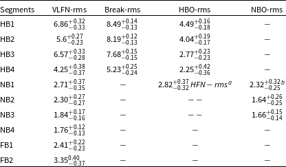
a LFN-rms
b LFN-rms
Table 9. Energy dependent rms values (in %) of BLN and HBO components in the PDS.
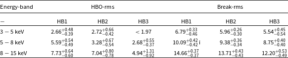
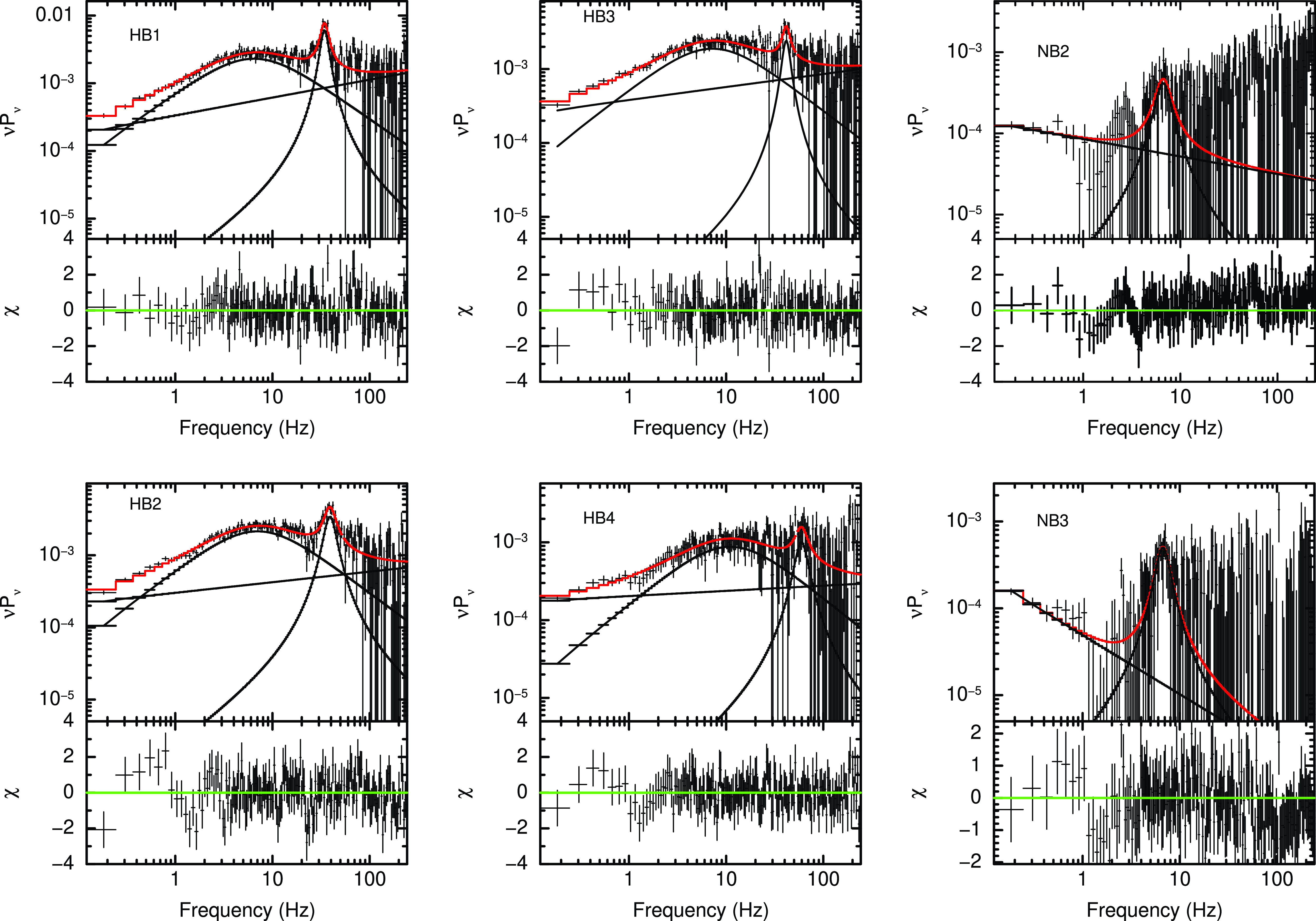
Figure 8. Figure shows the PDS for HID segments HB1, HB2, HB3 HB4, NB2 and NB3 in the energy band $3-50$
keV. In HB1, HB2 and HB3, a HBO is detected. A NBO is seen in the NB2 and NB3. The PDS for segments HB1,HB2 and HB3 are fitted with the combination of double Lorentzian and a power-law. The PDS for segments NB2 and NB3 are fitted with the combination of a power-law and a Lorentzian. Best-fit model along with the observed PDS has been shown in the figure.
$3-50$
keV. In HB1, HB2 and HB3, a HBO is detected. A NBO is seen in the NB2 and NB3. The PDS for segments HB1,HB2 and HB3 are fitted with the combination of double Lorentzian and a power-law. The PDS for segments NB2 and NB3 are fitted with the combination of a power-law and a Lorentzian. Best-fit model along with the observed PDS has been shown in the figure.
The inner disk is truncated far away from the NS ( $R_{eff} \sim 250-1600 $
km). Hence, the region between the inner disk rim and the magnetosphere is filled with hot coronal plasma. A large inner accretion disk radius (
$R_{eff} \sim 250-1600 $
km). Hence, the region between the inner disk rim and the magnetosphere is filled with hot coronal plasma. A large inner accretion disk radius ( $R_{eff}$
) has been reported in the Z-sources GX 340+0 (Bhargava et al., Reference Bhargava, Bhattacharyya, Homan and Pahari2023) and GX 5-1 (Shyam Prakash and Agrawal, Reference Shyam Prakash and Agrawal2024). Bhargava et al. (Reference Bhargava, Bhattacharyya, Homan and Pahari2023) suggests that probably the inner accretion disk is hidden inside a large corona. Other possibility is that the disk may be truncated due to radiation pressure. In both cases, the corona is not compact instead it is extended covering the NS surface and magnetosphere. We also note that the temperature changes by a smaller factor compared to the variation in the disk radius. Using the equation (Shakura and Sunyaev, Reference Shakura and Sunyaev1973)
$R_{eff}$
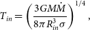
) has been reported in the Z-sources GX 340+0 (Bhargava et al., Reference Bhargava, Bhattacharyya, Homan and Pahari2023) and GX 5-1 (Shyam Prakash and Agrawal, Reference Shyam Prakash and Agrawal2024). Bhargava et al. (Reference Bhargava, Bhattacharyya, Homan and Pahari2023) suggests that probably the inner accretion disk is hidden inside a large corona. Other possibility is that the disk may be truncated due to radiation pressure. In both cases, the corona is not compact instead it is extended covering the NS surface and magnetosphere. We also note that the temperature changes by a smaller factor compared to the variation in the disk radius. Using the equation (Shakura and Sunyaev, Reference Shakura and Sunyaev1973)
 \begin{equation}T_{in} = \left(\frac{3GM \dot{M}}{8\pi R_{in}^3\sigma}\right)^{1/4},\end{equation}
we estimated the inner disk temperature and compared with observed temperature of the disk (see Figure 9). In this equation M is mass of the NS, $\dot{M}$
is mass accretion rate. From Figure 9, it can be seen that the trend of change in the estimated values of
$\dot{M}$
is mass accretion rate. From Figure 9, it can be seen that the trend of change in the estimated values of $kT_{in}$
and the fitted values of
$kT_{in}$
and the fitted values of $kT_{in}$
along the Z-track is similar. However, the the estimated and observed temperatures do not exactly match, suggesting that the nature of accretion disk may deviate from the standard accretion disk (Shakura and Sunyaev, Reference Shakura and Sunyaev1973) at high luminosities. The spectral modeling of emission from the source with tbabs*(diskbb+Comptb) favor a truncated disk scenario. The disk flow probably starts deviating from Keplerian to sub-Keplerian flow at the inner edge to satisfy the inner boundary conditions at the NS surface. The transition from a Keplerian to a sub-Keplerian flow creates centrifugal barrier (CB) at the transition point where matter starts piling up vertically forming a transition layer (TL) (Chakrabarti and Titarchuk, Reference Chakrabarti and Titarchuk1995; Chakrabarti, Reference Chakrabarti1997; Titarchuk, Lapidus, and Muslimov, Reference Titarchuk, Lapidus and Muslimov1998). The soft photons from the NS surface is up-scattered by the hot electrons present in the TL (Farinelli et al., Reference Farinelli, Titarchuk, Paizis and Frontera2008). The small illumination factor (
$kT_{in}$
along the Z-track is similar. However, the the estimated and observed temperatures do not exactly match, suggesting that the nature of accretion disk may deviate from the standard accretion disk (Shakura and Sunyaev, Reference Shakura and Sunyaev1973) at high luminosities. The spectral modeling of emission from the source with tbabs*(diskbb+Comptb) favor a truncated disk scenario. The disk flow probably starts deviating from Keplerian to sub-Keplerian flow at the inner edge to satisfy the inner boundary conditions at the NS surface. The transition from a Keplerian to a sub-Keplerian flow creates centrifugal barrier (CB) at the transition point where matter starts piling up vertically forming a transition layer (TL) (Chakrabarti and Titarchuk, Reference Chakrabarti and Titarchuk1995; Chakrabarti, Reference Chakrabarti1997; Titarchuk, Lapidus, and Muslimov, Reference Titarchuk, Lapidus and Muslimov1998). The soft photons from the NS surface is up-scattered by the hot electrons present in the TL (Farinelli et al., Reference Farinelli, Titarchuk, Paizis and Frontera2008). The small illumination factor ( $A\lt\lt1$
) for second Comptb suggests that emission from the disk is seen directly. Hence, the transition layer is geometrically thick and located between inner edge of accretion disk (which is truncated) and the NS magnetosphere. The photons from the NS are completely hidden and intercepted by an optically thick (
$A\lt\lt1$
) for second Comptb suggests that emission from the disk is seen directly. Hence, the transition layer is geometrically thick and located between inner edge of accretion disk (which is truncated) and the NS magnetosphere. The photons from the NS are completely hidden and intercepted by an optically thick ( $\tau \sim 3-5$
) and geometrically thick TL. The bulk flow parameter
$\tau \sim 3-5$
) and geometrically thick TL. The bulk flow parameter $\delta$
is zero, suggesting that the bulk flow is suppressed due to the strong radiation pressure at the vicinity of the NS. The bolometric unabsorbed luminosity in the energy range
$\delta$
is zero, suggesting that the bulk flow is suppressed due to the strong radiation pressure at the vicinity of the NS. The bolometric unabsorbed luminosity in the energy range $0.5-50$
keV of the source increases along the HB becoming highest at the hard apex and then again decreases along the Z-track. The disk and Comptonised luminosity follow a similar trend. Based on the multi-frequency observations of Cyg X-2, Hasinger et al. (Reference Hasinger, van der Klis, Ebisawa, Dotani and Mitsuda1990) argued that accretion rate monotonically increases from HB to NB and then FB. However, opposite scenario has also been proposed to explain the ‘Z’ tracks of Cyg-like Z-sources (Bałucinska-Church et al., Reference Bałucińska-Church, Schulz, Wilms, Gibiec, Hanke, Spencer, Rushton and Church2011). The Comptonisation flux show a systematic increase from HB1 to NB1. The location of inner edge of the disk is decided by balance between ram pressure and radiation pressure of Comptonised flux. The corona can be considered as a transition layer between inner edge of accretion disk and
$0.5-50$
keV of the source increases along the HB becoming highest at the hard apex and then again decreases along the Z-track. The disk and Comptonised luminosity follow a similar trend. Based on the multi-frequency observations of Cyg X-2, Hasinger et al. (Reference Hasinger, van der Klis, Ebisawa, Dotani and Mitsuda1990) argued that accretion rate monotonically increases from HB to NB and then FB. However, opposite scenario has also been proposed to explain the ‘Z’ tracks of Cyg-like Z-sources (Bałucinska-Church et al., Reference Bałucińska-Church, Schulz, Wilms, Gibiec, Hanke, Spencer, Rushton and Church2011). The Comptonisation flux show a systematic increase from HB1 to NB1. The location of inner edge of the disk is decided by balance between ram pressure and radiation pressure of Comptonised flux. The corona can be considered as a transition layer between inner edge of accretion disk and $R_{ISCO}$
. An increase in the radiation pressure or radiation drag may push the disk outwards. Indeed, the inner disk radius also increases from HB1 to NB1. The electron temperature of the corona shows slight decrease (4.47 to 3.97) and the optical depth does not show much variations from HB1 to NB1. However, the Comptonisation flux increases due to increase in its normalisation. Since the inner rim of the disk and outer edge of the TL is moving outwards, size of the corona increases. This suggests that the corona should become optically thin and hot as the source travels along the HB. The increase in the soft seed photon luminosity reverse this expected change in the corona and also explains the observed brightening of the corona from HB1 to NB1.
$R_{ISCO}$
. An increase in the radiation pressure or radiation drag may push the disk outwards. Indeed, the inner disk radius also increases from HB1 to NB1. The electron temperature of the corona shows slight decrease (4.47 to 3.97) and the optical depth does not show much variations from HB1 to NB1. However, the Comptonisation flux increases due to increase in its normalisation. Since the inner rim of the disk and outer edge of the TL is moving outwards, size of the corona increases. This suggests that the corona should become optically thin and hot as the source travels along the HB. The increase in the soft seed photon luminosity reverse this expected change in the corona and also explains the observed brightening of the corona from HB1 to NB1.
The reduction of coronal luminosity is observed from NB1 to FB2. Also, we note that the spectra become softer (or hard color decreases) and count rate decreases along this section of HID. The change in the hardness ratio is basically decided by the variation in the Comptonised component. The electron temperature decreases slightly (4.3 - 3.3 keV) and the optical depth shows slight decrease (4.4 to 3.4) from the segment NB1 to FB2. The Sco-like Z-source GX 17+2 has also shown similar behaviour in the NB (Agrawal, Nandi and Ramadevi, Reference Agrawal, Nandi and Ramadevi2020). In GX 17+2, the optical depth decreases and electron temperature remains almost constant along the NB. It was proposed that an increase in the seed photon supply from the boundary-layer or the NS surface causes a small fraction of coronal material to cool down and settle down in an underlying accretion disk. This mechanism leaves slightly less denser plasma cloud, explaining observed decrease in the optical depth along the NB. However, in the present case we note that the soft seed photons from the NS surface decreases along the NB and FB. The decrease in the luminosity with an increase in the mass accretion rate can be explained by increase in anisotropy of the X-ray emitting region causing decrease in the fraction of the X-ray flux emitted towards the observer’s line of sight. Most probably the height (H) of the corona is increasing and at the same time its shape is changing from TL with H/R $_{in}$ $\lt$
1 to slightly asymmetric flow with
$\lt$
1 to slightly asymmetric flow with $H/R_{in}$ $\sim$
1. This may explain the decrease in the optical depth (as volume of the corona increases and hence density decreases). The increased supply of seed photons from the NS surface, anticipated due to increase in accretion rate can cause decrease in the coronal temperature from NB1 to FB2. A decrease in the polarisation degree (PD) has been observed as the source moves HB to NB. The decrease in the scattering efficiency of the corona from from the hard apex to the lower NB can explain the observed decrease in the PD.
$\sim$
1. This may explain the decrease in the optical depth (as volume of the corona increases and hence density decreases). The increased supply of seed photons from the NS surface, anticipated due to increase in accretion rate can cause decrease in the coronal temperature from NB1 to FB2. A decrease in the polarisation degree (PD) has been observed as the source moves HB to NB. The decrease in the scattering efficiency of the corona from from the hard apex to the lower NB can explain the observed decrease in the PD.
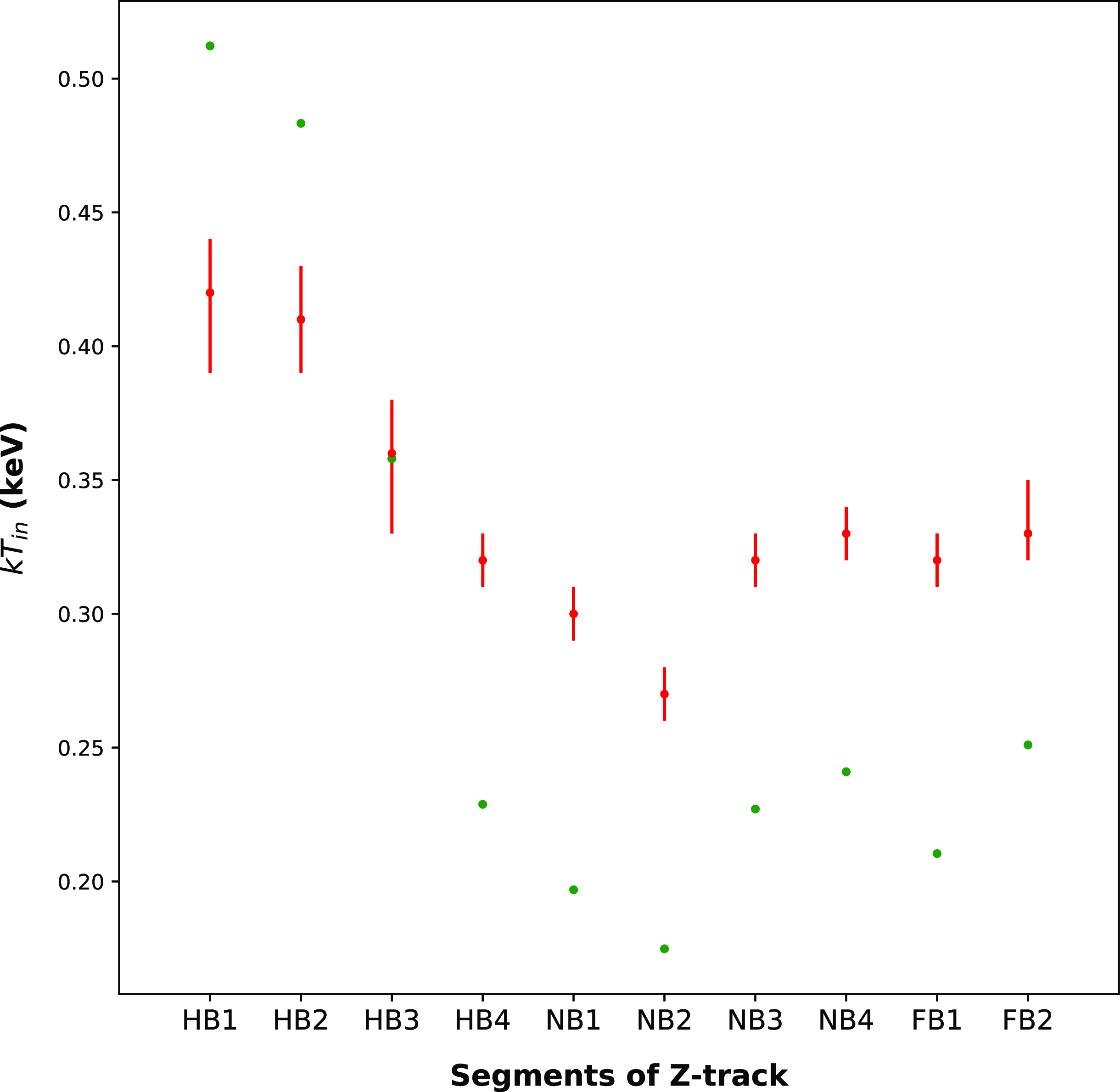
Figure 9. A comparison between the observed inner disk temperature and derived values. The estimated temperature values are denoted using green dots and the fitted values are shown using red dots with error.
We observe a dipping FB in this source, such a dipping behaviour has been observed in Z-sources, GX 340+0 (Jonker et al. 1998), GX 5-1 (Wijnands et al., Reference Wijnands, Méndez, van der Klis, Psaltis, Kuulkers and Lamb1998) and Cyg X-2 (Mondal et al., Reference Mondal, Dewangan, Pahari and Raychaudhuri2018). This source also has shown a dipping FB during its previous outburst (Homan et al. Reference Homan, van der Klis, Wijnands, Belloni, Fender, Klein-Wolt and Casella2007). The dipping FB in the source is associated with a reduced optical depth and a lower coronal temperature. This is opposite to behaviour observed in Cyg X-2 where the optical depth was found to increase during the X-ray dips (Mondal et al., Reference Mondal, Dewangan, Pahari and Raychaudhuri2018). Multi-wavelength study of Cyg X-2 suggested that the X-ray dip is caused by absorption of an extended coronal emission by the structure in the outer accretion disk (Bałucinska-Church et al., Reference Bałucińska-Church, Schulz, Wilms, Gibiec, Hanke, Spencer, Rushton and Church2011). Hence, changing corona geometry (X-ray emitting region becomes anisotropic in the FB) can explain the X-ray dips observed in the source.
This source has shown, HBOs, NBOs and a pair of kHz QPOs during the previous outburst (Homan et al., Reference Homan, van der Klis, Wijnands, Belloni, Fender, Klein-Wolt and Casella2007). The source exhibited kHz QPO pairs in Z-phase and single kHz QPO in atoll-phase (Sanna et al., Reference Sanna, Méndez, Altamirano, Homan, Casella, Belloni, Lin, van der Klis and Wijnands2010). In the Z-phase, kHz QPOs were weaker and broader compared to the atoll-phase. The timing properties of the source was studied in detail during the Cyg-like phase (Homan et al., Reference Homan, van der Klis, Wijnands, Belloni, Fender, Klein-Wolt and Casella2007) where the source exhibited dipping FB. It was noted that frequency of HBO increases and rms strength decreases along the HB. During AstroSat observation also the source was in Cyg-like phase and showed dipping FB, suggesting that temporal and spectral properties of the source should be similar. During the AstroSat observations the source exhibited HBOs in the frequency range $34-40$
Hz. The strength of the HBOs observed in the source decreases as the source travels from HB1 to HB3 and then they disappear as the source further moves down the Z-track. The Comptonisation flux increases from HB1 to HB4. However ratio of the Comptonisation flux and total flux decreases along the HB and hence the HBO rms is correlated with the percentage contribution of Comptonised emission to the total flux. Bu et al. (Reference Bu, Chen, Li, Qu, Belloni and Zhang2015) investigated the HBO properties of the source using all available RXTE observations of the source during its 2006 outburst. They also found that the HBO rms decreases from top-left of the HB to the hard-apex. The rms of the HBOs and the BLN component increases with increase in the photon energy from 4 to 12 keV (see Table 7). Energy dependent studies of HBOs of this source using data from RXTE satellite also provided a similar result in this source (Bu et al., Reference Bu, Chen, Li, Qu, Belloni and Zhang2015). GX 340+0 also shows increase in the HBO strength with increasing photon energy (Jonker et al. Reference Jonker, Wijnands, van der Klis, Psaltis, Kuulkers and Lamb1998). Hard nature of the HBOs and the BLN component suggests that their origin is linked with the hot corona around the compact object. We find a positive correlation between the break frequency and the HBO frequency, consistent with the previous observation of the source (Bu et al., Reference Bu, Chen, Li, Qu, Belloni and Zhang2015). Moreover, frequency resolved spectroscopy of the HBOs suggests that these oscillations are produced in the Comptonising region (Revnivtsev and Gilfanov, Reference Revnivtsev and Gilfanov2006).
$34-40$
Hz. The strength of the HBOs observed in the source decreases as the source travels from HB1 to HB3 and then they disappear as the source further moves down the Z-track. The Comptonisation flux increases from HB1 to HB4. However ratio of the Comptonisation flux and total flux decreases along the HB and hence the HBO rms is correlated with the percentage contribution of Comptonised emission to the total flux. Bu et al. (Reference Bu, Chen, Li, Qu, Belloni and Zhang2015) investigated the HBO properties of the source using all available RXTE observations of the source during its 2006 outburst. They also found that the HBO rms decreases from top-left of the HB to the hard-apex. The rms of the HBOs and the BLN component increases with increase in the photon energy from 4 to 12 keV (see Table 7). Energy dependent studies of HBOs of this source using data from RXTE satellite also provided a similar result in this source (Bu et al., Reference Bu, Chen, Li, Qu, Belloni and Zhang2015). GX 340+0 also shows increase in the HBO strength with increasing photon energy (Jonker et al. Reference Jonker, Wijnands, van der Klis, Psaltis, Kuulkers and Lamb1998). Hard nature of the HBOs and the BLN component suggests that their origin is linked with the hot corona around the compact object. We find a positive correlation between the break frequency and the HBO frequency, consistent with the previous observation of the source (Bu et al., Reference Bu, Chen, Li, Qu, Belloni and Zhang2015). Moreover, frequency resolved spectroscopy of the HBOs suggests that these oscillations are produced in the Comptonising region (Revnivtsev and Gilfanov, Reference Revnivtsev and Gilfanov2006).
In many models of QPOs, the kHz QPOs and HBOs are linked with the inner disk radius (Miller, Lamb, and Psaltis, Reference Miller, Lamb and Psaltis1998; Stella and Vietri, Reference Stella and Vietri1999). According to these models the upper kHz QPOs depends upon the location of inner edge of accretion disk. The observed kHz QPOs (Sanna et al. Reference Sanna, Méndez, Altamirano, Homan, Casella, Belloni, Lin, van der Klis and Wijnands2010) in the XTE J1701-462 gives $R_{in} \sim 20$
km. In the present case, disk is truncated away from the NS surface. If spectral nature of the source during the Z-phase of the previous outburst and the present outburst are similar then the origin of kHz QPOs can not be explained in the framework of these QPO models. Presently, we have detected only HBOs and NBOs in the Cyg-like Z-phase of the source.
$R_{in} \sim 20$
km. In the present case, disk is truncated away from the NS surface. If spectral nature of the source during the Z-phase of the previous outburst and the present outburst are similar then the origin of kHz QPOs can not be explained in the framework of these QPO models. Presently, we have detected only HBOs and NBOs in the Cyg-like Z-phase of the source.
The Lense-Thirring (LT) precession model has been proposed to explain the HBOs observed in NS-LMXBs and LFQPOs in black hole binaries (Ingram, Done, and Fragile, Reference Ingram, Done and Fragile2009). According to this model precession of radially extended hot central corona produces the observed QPOs in these two class of objects. The outer radius of the hot flow is decided by the truncation radius of the disk. The disk is truncated $\sim$
250-1100 km in the segments HB1 to HB4 sections of the Z-track. We take outer radius
$\sim$
250-1100 km in the segments HB1 to HB4 sections of the Z-track. We take outer radius $r_o = R_{eff}/R_g$
and inner radius
$r_o = R_{eff}/R_g$
and inner radius $r_i = R_{NS}/R_g$
of the hot radial flow. The LT precession frequency is computed using the formula (Ingram, Done, and Fragile, Reference Ingram, Done and Fragile2009)
$r_i = R_{NS}/R_g$
of the hot radial flow. The LT precession frequency is computed using the formula (Ingram, Done, and Fragile, Reference Ingram, Done and Fragile2009)
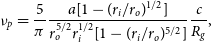 \begin{equation} \nu_p = \frac{5}{\pi} \frac{a[1-(r_i/r_o)^{1/2}]}{r_o^{5/2} r_i^{1/2} [1-(r_i/r_o)^{5/2}]} \frac{c}{R_g}, \end{equation}
where $R_g = 2.1$
km is gravitational radius of 1.4
$R_g = 2.1$
km is gravitational radius of 1.4 $M_\odot$
neutron star.
$M_\odot$
neutron star. $R_{NS} = 10$
km is NS radius. The above equation gives the QPO frequency of 0.2 Hz for
$R_{NS} = 10$
km is NS radius. The above equation gives the QPO frequency of 0.2 Hz for $R_{eff} =250$
km. Hence, this model can not explain the origin of the HBOs observed in the NS-LMXBs. Li et al. (Reference Li, Chen, Qu, Bu, Wang and Xu2014) observed a positive correlation between the inner disk radius and the HBO frequency. We also observed a similar correlation, which is hard to explain in the framework of the LT precession model. Probably, the LT precesses diferentially with a higher precession frequency at the inner region of TL compared to outer region (van den Eijnden, Ingram, and Uttley Reference van den Eijnden, Ingram and Uttley2016; Huang et al., Reference Huang, Qu, Zhang, Bu, Chen, Tao and Zhang2018). Here, we can assume that TL is slightly warped where height of TL is higher in the inner region compared to that in outer region. Hence more modulation is produced by the faster precessing inner region.
$R_{eff} =250$
km. Hence, this model can not explain the origin of the HBOs observed in the NS-LMXBs. Li et al. (Reference Li, Chen, Qu, Bu, Wang and Xu2014) observed a positive correlation between the inner disk radius and the HBO frequency. We also observed a similar correlation, which is hard to explain in the framework of the LT precession model. Probably, the LT precesses diferentially with a higher precession frequency at the inner region of TL compared to outer region (van den Eijnden, Ingram, and Uttley Reference van den Eijnden, Ingram and Uttley2016; Huang et al., Reference Huang, Qu, Zhang, Bu, Chen, Tao and Zhang2018). Here, we can assume that TL is slightly warped where height of TL is higher in the inner region compared to that in outer region. Hence more modulation is produced by the faster precessing inner region.
Recently phase resolved polarimetry of a strong LFQPOs, seen in the transient blackhole candidate Swift J1727.8–1613, has been carried out (Zhao et al., Reference Zhao, Tao, Li, Zhang, Feng, Ge and Ji2024). No modulation in the polarisation degree and the polarisation angle is observed with the QPO phase. Hence, polarimetric observations are also not in favor of the LT precession model. LT precession model of jet and inner disk ring has been used to explain the LFQPOs seen in Swift J1727.8-1613 (Yu, Bu, Zhang, et al. Reference Yu, Bu, Zhang, Liu, Zhang, Ducci and Tao2024). LFQPO in the hard X-rays was detected in Swift J1727.8-1613 with AstroSat (Nandi et al. Reference Nandi, Das, Majumder, Katoch, Antia and Shah2024). It was suggested that the oscillations in a hot and dense downstream flow at the vicinity of the blackhole produces the QPOs (Nandi et al., Reference Nandi, Das, Majumder, Katoch, Antia and Shah2024).
IGR 17480-2446, which is a transient mili-second pulsars with 11 Hz pulse period, exhibited HBOs ( $35 - 50$
Hz) and kHz QPOs (Barret, 2012; Altamirano et al., Reference Altamirano, Ingram, van der Klis, Wijnands, Linares and Homan2012). This source also showed transition from atoll to luminous Z-phase (Chakraborty, Bhattacharyya, and Mukherjee, Reference Chakraborty, Bhattacharyya and Mukherjee2011). To explain the nature of HBO in this source the Altamirano et al. (Reference Altamirano, Ingram, van der Klis, Wijnands, Linares and Homan2012) suggested that precession due to frame dragging alone is not sufficient to explain the observed frequency of HBOs. They proposed that a warp is induced by magnetic field in the hot inner flow and that precesses with frequency
$35 - 50$
Hz) and kHz QPOs (Barret, 2012; Altamirano et al., Reference Altamirano, Ingram, van der Klis, Wijnands, Linares and Homan2012). This source also showed transition from atoll to luminous Z-phase (Chakraborty, Bhattacharyya, and Mukherjee, Reference Chakraborty, Bhattacharyya and Mukherjee2011). To explain the nature of HBO in this source the Altamirano et al. (Reference Altamirano, Ingram, van der Klis, Wijnands, Linares and Homan2012) suggested that precession due to frame dragging alone is not sufficient to explain the observed frequency of HBOs. They proposed that a warp is induced by magnetic field in the hot inner flow and that precesses with frequency $\nu_{mag}$
. The magnetic precession depends on the magnetic moment
$\nu_{mag}$
. The magnetic precession depends on the magnetic moment $\mu$
. The net precession frequency is combination of magnetic and frame dragging effects.
$\mu$
. The net precession frequency is combination of magnetic and frame dragging effects.
As HBOs are linked to the Comptonising component, other kind of oscillations in the corona can produce these frequencies. Cabanac et al. (Reference Cabanac, Henri, Petrucci, Malzac, Ferreira and Belloni2010) proposed the oscillating hot corona model to explain the low frequency QPOs seen in X-ray binaries. They suggested that a magneto-acoustic wave propagating in the hot corona can produce resonant peaks in the PDS.
Another popular model proposed to explain the origin of the QPOs is two-oscillator model (Osherovich and Titarchuk, Reference Osherovich and Titarchuk1999). According to this model hot, large and inhomogeneous blobs are formed at the outer edge of the TL and injected into the NS magnetosphere. If the blobs formed at the outer edge of the TL are rotating differentially, having higher angular velocity at inner edge compared to outer edge. These blobs with certain velocity distributions are injected to the NS magnetosphere from the inner edge of TL. Such blobs under influence of Coriolis force behave as Keplerian oscillators with two modes : radial and vertical (Osherovich and Titarchuk, Reference Osherovich and Titarchuk1999). The radial mode is identified with upper kHz QPO and the mode perpendicular to the accretion disk produces the HBOs. The lower kHz QPO is identified with the Keplerian frequency of the blobs at the inner edge of TL. These hot plasma balls intercept the photons from the NS surface and up-scatter them. Hence, we expect rms strength of the HBOs to be positively correlated with the energy of photons. A positive correlation seen between the HBO-rms and the photon energy support this scenario. The radiation pressure increases as the source moves from HB1 to HB4 due to increase in the source luminosity. The increasing radiation pressure disrupts the flow of hot blobs responsible for HBOs. Therefore, HBOs become weaker as the source moves down the HB and disappear as source moves further along the Z-track. The observed LFQPOs (HBOs and NBOs) can also be explained in the framework of oscillating shock wave model (Molteni, Sponholz, and Chakrabarti, Reference Molteni, Sponholz and Chakrabarti1996). In this model, shock oscillates radially with a time period equal to the cooling time scale of the corona. NBOs at frequency $\sim$
6.6 Hz are seen in the middle and lower NB. The frequency of NBOs always lies in the narrow range (
$\sim$
6.6 Hz are seen in the middle and lower NB. The frequency of NBOs always lies in the narrow range ( $\sim 5-7 $
Hz), suggesting that they are linked with some kind of fundamental frequency of accretion flow close to the NS (Hasinger, Reference Hasinger1987). According model proposed by Hasinger (Reference Hasinger1987), at high accretion rate the inomogeneous plasma is accreted at the free fall velocity and causes density fluctuations in a layer above the NS surface. The density fluctuations propagates with local sound speed on the NS surface given by
$\sim 5-7 $
Hz), suggesting that they are linked with some kind of fundamental frequency of accretion flow close to the NS (Hasinger, Reference Hasinger1987). According model proposed by Hasinger (Reference Hasinger1987), at high accretion rate the inomogeneous plasma is accreted at the free fall velocity and causes density fluctuations in a layer above the NS surface. The density fluctuations propagates with local sound speed on the NS surface given by
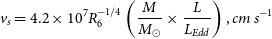 \begin{equation}v_s = 4.2 \times 10^7 R_6^{-1/4} \left(\frac{M}{M_\odot} \times \frac{L}{L_{Edd}} \right), cm ~ s^{-1}\end{equation}
where $R_6$
is NS radius in units of
$R_6$
is NS radius in units of $10^6$
cm (Hasinger, Reference Hasinger1987). The propagation of these fluctuations on the NS surface produces NBOs. Due to variations in mass accretion rate, a spectrum of density fluctuations will be produced, the fundamental tone of which is given by
$10^6$
cm (Hasinger, Reference Hasinger1987). The propagation of these fluctuations on the NS surface produces NBOs. Due to variations in mass accretion rate, a spectrum of density fluctuations will be produced, the fundamental tone of which is given by
 \begin{equation}\nu_s = \frac{v_s}{2\pi R} Hz,\end{equation}
where R is the neutron star radius. It is clear that the $\nu_s$
depends upon the NS radius, mass accretion rate (which is always close to Eddington limit for 1.4 solar mass NS) and mass of the NS (Hasinger, Reference Hasinger1987). Therefore, the NBO frequency lies in a narrow range around 6 Hz. Alternatively, it can be produced by acoustic oscillations of a spherical shell around the NS (Titarchuk et al. Reference Titarchuk, Bradshaw, Geldzahler and Fomalont2001). In this scenario, transition layer can become spherical at high accretion rate. The spherical shell oscillates with a frequency,
$\nu_s$
depends upon the NS radius, mass accretion rate (which is always close to Eddington limit for 1.4 solar mass NS) and mass of the NS (Hasinger, Reference Hasinger1987). Therefore, the NBO frequency lies in a narrow range around 6 Hz. Alternatively, it can be produced by acoustic oscillations of a spherical shell around the NS (Titarchuk et al. Reference Titarchuk, Bradshaw, Geldzahler and Fomalont2001). In this scenario, transition layer can become spherical at high accretion rate. The spherical shell oscillates with a frequency,
 \begin{equation}\nu_s = \frac{fv_s}{L} Hz,\end{equation}
where, f = 0.5 or $1/2\pi$
, depending upon the boundary conditions and L is size of the spherical shell. In this model of NBO, the oscillation frequency depends upon size of the spherical shell which can vary from source to source and hence suffers difficulties. Alternatively the observed NBOs can also be explained in the framework of oscillating corona model (Cabanac et al. Reference Cabanac, Henri, Petrucci, Malzac, Ferreira and Belloni2010).
$1/2\pi$
, depending upon the boundary conditions and L is size of the spherical shell. In this model of NBO, the oscillation frequency depends upon size of the spherical shell which can vary from source to source and hence suffers difficulties. Alternatively the observed NBOs can also be explained in the framework of oscillating corona model (Cabanac et al. Reference Cabanac, Henri, Petrucci, Malzac, Ferreira and Belloni2010).
Acknowledgement
Author thanks GH, SAG; DD, PDMSA, and Director URSC for encouragement and continuous support to carry out this research. Author thanks anonymous reviewer for useful and constructive suggestions which helped to improve the quality of the manuscript. This work has used the data from the LAXPC Instruments developed at TIFR, Mumbai and the LAXPC POC at TIFR is thanked for verifying and releasing the data via the ISSDC data archive. We thank the AstroSat Science Support Cell hosted by IUCAA and TIFR for providing the LaxpcSoft software which we used for LAXPC data analysis. This work has used the data from the Soft X-ray Telescope (SXT) developed at TIFR, Mumbai, and the SXT POC at TIFR is thanked for verifying and releasing the data and providing the necessary software tools.
Data availability statement
Data underlying this article are available at AstroSat-ISSDC website https://www.astrobrowse.issdc.gov.in/astroarchive/archive.


 Open access