


1. Introduction
Fast Radio Bursts (FRBs) are a recently discovered class of astrophysical transients of predominantly extragalactic origin. They are highly energetic bursts at radio wavelengths, lasting only a few milliseconds and detectable from the distant Universe (up to and perhaps beyond redshift $z=1$
, e.g. FRB 20220610A with
$z=1$
, e.g. FRB 20220610A with $z=1.016 \pm 0.002$
reported by Ryder et al. Reference Ryder2023), and as such have emerged as a frontier field of modern astrophysics (reviews Petroff et al. Reference Petroff, Hessels and Lorimer2022; Pilia Reference Pilia2021; Cordes & Chatterjee Reference Cordes and Chatterjee2019). In just over 15 years, the number of FRBs ‘sky-rocketed’ from a single Lorimer Burst (Lorimer et al. Reference Lorimer, Bailes, McLaughlin, Narkevic and Crawford2007) through a few tens of detections with Parkes (Murriyang) radio telescope (Thornton et al. Reference Thornton2013) to several hundreds (CHIME/FRB Collaboration et al. 2021). The interferometric localisations and associations with host galaxies have enabled redshift measurements and ultimately confirmed the extra-galactic origin of FRBs (Chatterjee et al. Reference Chatterjee2017; Tendulkar et al. Reference Tendulkar2017; Ravi et al. Reference Ravi2019; Bannister et al. Reference Bannister2019b; Prochaska et al. Reference Prochaska2019; Marcote et al. Reference Marcote2020). Furthermore, the interferometric localisations of several FRBs by the Commensal Realtime ASKAP Fast Transients (CRAFT) survey (Macquart et al. Reference Macquart2010) on the Australian Square Kilometre Array Pathfinder (ASKAP) at 1.4 GHz also enabled measurements of the electron content of the Universe and established the Macquart relation between the dispersion measure (DM) and redshift (Macquart et al. Reference Macquart2020). With the increasing number of localised detections from ASKAP CRAFT, Deep Synoptic Array (Ravi et al. Reference Ravi2023, DSA-110Footnote
a
;) and other instruments, the precision of these measurements and significance of FRBs as cosmological probes will continue to increase. In addition to using FRBs as cosmological tools, there have been ongoing efforts to understand their progenitors and underlying physical mechanisms. In the early days of FRB research, Arecibo telescope discovered the first repeating FRB 121102 (Spitler et al. Reference Spitler2014), which led to the hypothesis that there are two distinct populations of FRBs: namely, repeating, and one-off.
$z=1.016 \pm 0.002$
reported by Ryder et al. Reference Ryder2023), and as such have emerged as a frontier field of modern astrophysics (reviews Petroff et al. Reference Petroff, Hessels and Lorimer2022; Pilia Reference Pilia2021; Cordes & Chatterjee Reference Cordes and Chatterjee2019). In just over 15 years, the number of FRBs ‘sky-rocketed’ from a single Lorimer Burst (Lorimer et al. Reference Lorimer, Bailes, McLaughlin, Narkevic and Crawford2007) through a few tens of detections with Parkes (Murriyang) radio telescope (Thornton et al. Reference Thornton2013) to several hundreds (CHIME/FRB Collaboration et al. 2021). The interferometric localisations and associations with host galaxies have enabled redshift measurements and ultimately confirmed the extra-galactic origin of FRBs (Chatterjee et al. Reference Chatterjee2017; Tendulkar et al. Reference Tendulkar2017; Ravi et al. Reference Ravi2019; Bannister et al. Reference Bannister2019b; Prochaska et al. Reference Prochaska2019; Marcote et al. Reference Marcote2020). Furthermore, the interferometric localisations of several FRBs by the Commensal Realtime ASKAP Fast Transients (CRAFT) survey (Macquart et al. Reference Macquart2010) on the Australian Square Kilometre Array Pathfinder (ASKAP) at 1.4 GHz also enabled measurements of the electron content of the Universe and established the Macquart relation between the dispersion measure (DM) and redshift (Macquart et al. Reference Macquart2020). With the increasing number of localised detections from ASKAP CRAFT, Deep Synoptic Array (Ravi et al. Reference Ravi2023, DSA-110Footnote
a
;) and other instruments, the precision of these measurements and significance of FRBs as cosmological probes will continue to increase. In addition to using FRBs as cosmological tools, there have been ongoing efforts to understand their progenitors and underlying physical mechanisms. In the early days of FRB research, Arecibo telescope discovered the first repeating FRB 121102 (Spitler et al. Reference Spitler2014), which led to the hypothesis that there are two distinct populations of FRBs: namely, repeating, and one-off.
In the first few years, the FRB field was dominated by dish telescopes operating at GHz frequencies. Although the initial efforts at sub-GHz frequencies were unsuccessful, eventually FRBs were detected at 800 MHz (Caleb et al. Reference Caleb2017) by the UTMOST telescope (Bailes et al. Reference Bailes2017). In 2018, Canadian Hydrogen Intensity Mapping Experiment (CHIME) came online, started to detect many FRBs, and became a true northern hemisphere ‘FRB factory’. In 2021, CHIME published a catalogue of 536 one-off and 18 repeating FRBs (CHIME/FRB Collaboration et al. 2021, 2020a) at 400–800 MHz, and more recently confirmed another 25 repeating FRBs (Andersen et al. Reference Andersen2023). Their large sample of FRBs enabled statistical and morphological studies of the FRB population (Pleunis et al. Reference Pleunis2021b). These results indicate that physical properties of one-off and repeating FRBs are different, which suggests different underlying populations of sources or differences in the local environments of the two classes. The main limitation of the CHIME telescope has been the localisation accuracy, though the upcoming outrigger project will provide sub-arcsecond localisation precision (Sanghavi et al. Reference Sanghavi2023) and guarantee that CHIME will also contribute significantly more to cosmological studies. Intriguingly, many CHIME FRBs detected down to 400 MHz appear not to be scattered (modulo CHIME’s limitations to measure scattering), which suggests that many of the CHIME FRBs should also be detectable at frequencies below 400 MHz.
1.1. FRB searches at frequencies below 350 MHz
Despite the success of CHIME at frequencies above 400 MHz, and ongoing efforts at lower frequencies, there have only been a few FRB detections at frequencies below 400 MHz. The initial searches by LOFAR (Coenen et al. Reference Coenen2014; Karastergiou et al. Reference Karastergiou2015) did not detect any FRBs. Similarly, efforts using the Murchison Widefield Array (MWA; Tingay et al. Reference Tingay2013; Wayth et al. Reference Wayth2018), failed mainly because of the limited on-sky time and signal processing constraints (time and frequency resolutions $\ge$
0.5 s and 1.28 MHz, respectively) that limited sensitivity to short pulses to
$\ge$
0.5 s and 1.28 MHz, respectively) that limited sensitivity to short pulses to $\gtrsim$
500 Jy ms (Rowlinson et al. Reference Rowlinson2016; Keane et al. Reference Keane2016; Tingay et al. Reference Tingay2015). Table 1 summarises these earlier non-targeted FRB searches at low frequencies.
$\gtrsim$
500 Jy ms (Rowlinson et al. Reference Rowlinson2016; Keane et al. Reference Keane2016; Tingay et al. Reference Tingay2015). Table 1 summarises these earlier non-targeted FRB searches at low frequencies.
Table 1. Summary of past, present, and future non-targeted wide-field and all-sky searches for low-frequency FRBs. Only Parent et al. (Reference Parent2020) (1 $^\mathrm{st}$
line) detected one FRB.
$^\mathrm{st}$
line) detected one FRB.
 $^\mathrm{a}$
Telescopes: G – GBT (100 m), J – Lovell telescope at Jodrell Bank (76 m), L – LOFAR, M – MWA (
$^\mathrm{a}$
Telescopes: G – GBT (100 m), J – Lovell telescope at Jodrell Bank (76 m), L – LOFAR, M – MWA ( $\sim$
60 m), C – all-sky FRB monitor CHASM implemented on SKA-Low stations (effective size 34 m at 100 MHz and 20 m at 200 MHz) described by Sokolowski et al. (Reference Sokolowski, Price and Wayth Randall2022a). The values in brackets are dish diameters or equivalent for the aperture arrays.
$\sim$
60 m), C – all-sky FRB monitor CHASM implemented on SKA-Low stations (effective size 34 m at 100 MHz and 20 m at 200 MHz) described by Sokolowski et al. (Reference Sokolowski, Price and Wayth Randall2022a). The values in brackets are dish diameters or equivalent for the aperture arrays. $^\mathrm{b}$
Figure of merit M = FoV
$^\mathrm{b}$
Figure of merit M = FoV $\times$ $\text{F}^{-3/2} \times$ $\text{T}_{obs} / \delta t$
(equation (6)) as defined in Cordes et al. (Reference Cordes, Lazio and McLaughlin2004), Cordes (Reference Cordes, Bridle, Condon and Hunt2008), Hessels et al. (Reference Hessels, Stappers, van Leeuwen, Saikia, Green, Gupta and Venturi2009), Macquart et al. (Reference Macquart2010). Here, M was divided by
$\text{T}_{obs} / \delta t$
(equation (6)) as defined in Cordes et al. (Reference Cordes, Lazio and McLaughlin2004), Cordes (Reference Cordes, Bridle, Condon and Hunt2008), Hessels et al. (Reference Hessels, Stappers, van Leeuwen, Saikia, Green, Gupta and Venturi2009), Macquart et al. (Reference Macquart2010). Here, M was divided by $\text{M}_0$
, where
$\text{M}_0$
, where $\text{T}_{obs}$
is the observing time, and
$\text{T}_{obs}$
is the observing time, and $\delta t$
is the time resolution.
$\delta t$
is the time resolution. $M_0$
is M calculated for survey parameters of the survey by Parent et al. (Reference Parent2020), which detected 1 FRB in about 174 days. This figure of merit increases with the increasing FoV, sensitivity, total observing time, and also with the improved time resolution (
$M_0$
is M calculated for survey parameters of the survey by Parent et al. (Reference Parent2020), which detected 1 FRB in about 174 days. This figure of merit increases with the increasing FoV, sensitivity, total observing time, and also with the improved time resolution ( $\delta t$
). Instead of detecting a single pulse during observing time
$\delta t$
). Instead of detecting a single pulse during observing time $T_{obs}$
, the higher time resolution enables detection of multiple (
$T_{obs}$
, the higher time resolution enables detection of multiple ( $\sim T_{obs} / \delta t$
) short pulses (
$\sim T_{obs} / \delta t$
) short pulses ( $\le \delta t$
) leading to more FRB detections.
$\le \delta t$
) leading to more FRB detections. $^\mathrm{c}$
The exact frequency range is 210.56 to 223.36 MHz.
$^\mathrm{c}$
The exact frequency range is 210.56 to 223.36 MHz. $^\mathrm{d}$
10
$^\mathrm{d}$
10 $\sigma$
threshold.
$\sigma$
threshold. $^\mathrm{e}$
Above elevation 25°.
$^\mathrm{e}$
Above elevation 25°.
Between 2017 and 2019, Sokolowski et al. (Reference Sokolowski2018) conducted an MWA campaign and co-observed (shadowed) the ASKAP field of view (FoV). During these observations ASKAP detected several FRBs, and two of them during favourable nighttime. Unfortunately, calibration of daytime MWA data was very difficult until an observing strategy placing the Sun in the null of the primary beam was implemented in late 2019 (Hancock et al. Reference Hancock2019). However, it turned out that neither of these two ASKAP FRBs was simultaneously (after correcting for dispersion delay) detected in the 0.5-s/1.28 MHz images from the MWA. The upper limit on flux density of these FRBs at 200 MHz led to constraints on the properties of the immediate surroundings of the FRB sources (e.g. on the size of the absorbing region) demonstrating the potential applications of the low-frequency observations (including non-detections). More recently, Tian et al. (Reference Tian2023b) used archival MWA high-time resolution data from the Voltage Capture System (VCS; Tremblay et al. Reference Tremblay2015) to look for pulses from a modest sample of FRBs (one ASKAP and four CHIME). Although they did not detect any pulses from these FRBs, similar targeted searches with the MWA and other low-frequency telescopes have significant potential to detect low-frequency pulses from repeating FRBs.
This was the case of one of the CHIME repeating FRBs 20180916B with a regular (hence predictable) activity period, which was detected by LOFAR (Pleunis et al. Reference Pleunis2021a; Pastor-Marazuela et al. Reference Pastor-Marazuela2021) at frequencies down to even 110 MHz – the first ever FRB detection below 300 MHz. Commensal observations of FRB 20180916B with CHIME, LOFAR and Apertif reported by Maan & van Leeuwen (Reference Maan and van Leeuwen2017) revealed that low-frequency emission was usually not detected when high-frequency emission was and vice versa, which is a possible explanation to earlier MWA non-detections of ASKAP FRBs by Sokolowski et al. (Reference Sokolowski2018). This so-called chromaticity window further supports the need to conduct independent searches for low-frequency FRBs, as the low-frequency signals may not be simultaneous with bursts at higher frequencies. Additionally, a one-off FRB 20200125A was discovered by the Green Bank Telescope (GBT) at 350 MHz (Parent et al. Reference Parent2020). These detections, together with CHIME FRBs extending down to 400 MHz, ultimately prove that FRBs can be detected at low radio frequencies.
1.2. FRB progenitors and models
Although the field has achieved significant progress on both observational and theoretical fronts (see Petroff et al. Reference Petroff, Hessels and Lorimer2022 for the recent review), physical mechanisms and FRB progenitors remain unexplained. A detailed summary of FRB models exceeds the scope of this paper but very good reviews of existing theoretical models can be found in Section 9 of Petroff et al. (Reference Petroff, Hessels and Lorimer2019) or in the FRB Theory CatalogueFootnote
b
(Platts et al. Reference Platts, Weltman, Walters, Tendulkar, Gordin and Kandhai2019). In short, the leading models for repeating FRBs relate them to magnetars (Metzger et al. Reference Metzger, Berger and Margalit2017; Margalit et al. Reference Margalit, Metzger, Berger, Nicholl, Eftekhari and Margutti2018), which are highly magnetised ( $\sim$ $10^{15}$
G) neutron stars (NSs) (e.g. Liu Reference Liu2018). Such long-lived stable magnetars can produce coherent radio pulses in a similar way to pulsars (dipole radiation) and be observed as repeating FRBs during their activity periods.
$10^{15}$
G) neutron stars (NSs) (e.g. Liu Reference Liu2018). Such long-lived stable magnetars can produce coherent radio pulses in a similar way to pulsars (dipole radiation) and be observed as repeating FRBs during their activity periods.
On the other hand, one-off FRBs are hypothesised to be produced in cataclysmic events, such as a collapse of a super-massive NS (e.g. Falcke & Rezzolla Reference Falcke and Rezzolla2014) as its rotation slows down due to magnetic braking. A super-massive NS can be formed in a cataclysmic event like an NS-NS merger (Totani Reference Totani2013; Chu et al. Reference Chu, Howell, Rowlinson, Gao, Zhang, Tingay, Boër and Wen2016; Zhang Reference Zhang2014; Metzger Reference Metzger2017) leading to a super-massive short-lived (seconds to hours) magnetar, which emits coherent radio bursts during its short lifetime and ultimately collapses to a black hole (Rowlinson & Anderson Reference Rowlinson and Anderson2019; Rowlinson et al. Reference Rowlinson2023).
Hence, magnetars are one of the main contenders for progenitors of both repeating and at least some non-repeating FRB. The magnetar model is strongly supported by the detections of FRB-like $\sim$
MJy radio pulses from the Galactic Soft Gamma Repeater SGR 1935+2154 (Bochenek et al. Reference Bochenek, Ravi, Belov, Hallinan, Kocz, Kulkarni and McKenna2020; CHIME/FRB Collaboration et al. 2020b), which was the only FRB-like event observed at other electromagnetic wavelengths. On the other hand, the more recent detection of FRB 20200120E (Kirsten et al. Reference Kirsten2022) pinpointed to a globular cluster (GC) slightly challenges the magnetar model as this kind of young NS is not expected to be present in GCs. An alternative model for FRBs is that they are due to extremely bright and short (even ns duration) pulses similar to so-called supergiant pulses emitted by pulsars like PSR B0531+21 (aka Crab) (Cordes & Wasserman Reference Cordes and Wasserman2016; Connor et al. Reference Connor, Pen and Oppermann2016).
$\sim$
MJy radio pulses from the Galactic Soft Gamma Repeater SGR 1935+2154 (Bochenek et al. Reference Bochenek, Ravi, Belov, Hallinan, Kocz, Kulkarni and McKenna2020; CHIME/FRB Collaboration et al. 2020b), which was the only FRB-like event observed at other electromagnetic wavelengths. On the other hand, the more recent detection of FRB 20200120E (Kirsten et al. Reference Kirsten2022) pinpointed to a globular cluster (GC) slightly challenges the magnetar model as this kind of young NS is not expected to be present in GCs. An alternative model for FRBs is that they are due to extremely bright and short (even ns duration) pulses similar to so-called supergiant pulses emitted by pulsars like PSR B0531+21 (aka Crab) (Cordes & Wasserman Reference Cordes and Wasserman2016; Connor et al. Reference Connor, Pen and Oppermann2016).
Although there is a general consensus that FRBs are produced by a coherent emission process, the exact radiation mechanisms are yet to be determined. In pulsar-like models, FRBs are produced by coherent emission processes occurring in the magnetosphere close ( $\lesssim$ $10^4$
km) to the surface of NS via magnetic reconnection (e.g. Lyutikov Reference Lyutikov2021) or curvature radiation (Kumar et al. Reference Kumar, Lu and Bhattacharya2017). On the other hand, in GRB-like models, coherent radio pulses are generated further away from the surface (
$10^4$
km) to the surface of NS via magnetic reconnection (e.g. Lyutikov Reference Lyutikov2021) or curvature radiation (Kumar et al. Reference Kumar, Lu and Bhattacharya2017). On the other hand, in GRB-like models, coherent radio pulses are generated further away from the surface ( $\gtrsim$ $10^5$
km) of NS via synchrotron maser mechanism in the forward shock of the flare of material ejected from a magnetar as it collides with the surrounding medium (Metzger et al. Reference Metzger, Margalit and Sironi2019). Comprehensive discussions can be found in the recent reviews by Petroff et al. (Reference Petroff, Hessels and Lorimer2022) and Pilia (Reference Pilia2021).
$10^5$
km) of NS via synchrotron maser mechanism in the forward shock of the flare of material ejected from a magnetar as it collides with the surrounding medium (Metzger et al. Reference Metzger, Margalit and Sironi2019). Comprehensive discussions can be found in the recent reviews by Petroff et al. (Reference Petroff, Hessels and Lorimer2022) and Pilia (Reference Pilia2021).
The same physical processes can also produce low-frequency radio signals ( $\lesssim$
300 MHz). However, radio signals at these frequencies may be suppressed by several mechanisms. At frequencies below plasma frequency
$\lesssim$
300 MHz). However, radio signals at these frequencies may be suppressed by several mechanisms. At frequencies below plasma frequency $\lesssim$
90 MHz they are quenched by plasma absorption, while at frequencies 90 MHz
$\lesssim$
90 MHz they are quenched by plasma absorption, while at frequencies 90 MHz $\,\lesssim \nu \lesssim$
300 MHz by free–free absorption in the NS’s dense immediate surroundings or ejected material (Pilia Reference Pilia2021). Therefore, detection of low-frequency FRBs may be possible only in low density environments where absorption is negligible, which may be the case at least in some progenitor systems, like FRB 190816B (Pleunis et al. Reference Pleunis2021a) and 200125A (Parent et al. Reference Parent2020).
$\,\lesssim \nu \lesssim$
300 MHz by free–free absorption in the NS’s dense immediate surroundings or ejected material (Pilia Reference Pilia2021). Therefore, detection of low-frequency FRBs may be possible only in low density environments where absorption is negligible, which may be the case at least in some progenitor systems, like FRB 190816B (Pleunis et al. Reference Pleunis2021a) and 200125A (Parent et al. Reference Parent2020).
FRB 180916B was detected in a targeted LOFAR search for low-frequency pulses from a CHIME repeating FRB with a known 16-day periodicity. As discussed earlier, repeating FRBs are believed to be due to stable magnetars, while their periodicity may be caused by interactions with the stellar wind from a companion star in the binary system with a massive/NS (Ioka & Zhang Reference Ioka and Zhang2020; Lyutikov et al. Reference Lyutikov, Barkov and Giannios2020) or precession of the magnetar’s spin axis (Zanazzi & Lai Reference Zanazzi and Lai2020; Tong et al. Reference Tong, Wang and Wang2020). Both models predict frequency dependent activity window and other characteristics which can be tested by simultanous observations at high and low frequencies (Pastor-Marazuela et al. Reference Pastor-Marazuela2021).
Finally, the most promising physical scenario leading to one-off low-frequency FRBs are events associated with short Gamma-Ray Bursts (SGRBs), which are also linked to NS-NS mergers. SGRBs seem to occur in low density environments (Fong et al. Reference Fong, Berger, Margutti and Zauderer2015). Hence, low-frequency radio signals produced at various stages of NS-NS merger can avoid absorption and be detected by low-frequency radio telescopes (Rowlinson & Anderson Reference Rowlinson and Anderson2019). A potential association of a coherent radio pulse with short GRB 201006A was recently reported by Rowlinson et al. (Reference Rowlinson2023).
1.3. A hunt for bright, nearby FRBs
Similarly to other astrophysical phenomena (e.g. Gamma-Ray Bursts (GRBs)) multi-wavelength observations may hold the key to explaining the FRB enigma. However, except the special case of the Galactic FRB from SGR 1935+2154, so far no FRB has been detected at other electromagnetic wavelengths than radio. Detection of more Galactic FRB-like events linked to magnetars, young NSs or other objects will provide essential observational evidence to support or disfavour theoretical models of FRBs.
The best candidates for the first multi-wavelength detections are bright FRBs from the local Universe. Therefore, nearby FRBs are of great interest for detailed studies of FRB host galaxies, progenitors and local environments. Accurate localisations of such nearby FRBs may pinpoint their host galaxies and even specific objects within host galaxies (e.g. Kirsten et al. Reference Kirsten2022) which will uncover information about their progenitors. Fast and precise localisation of bright nearby FRBs can lead to detections over a broad range of the electromagnetic spectrum (optical, gamma, X-rays etc) and/or in other messengers such as gravitational waves (GWs), which will be particularly useful for explaining the underlying physics. James et al. (Reference James, Prochaska, Macquart, North-Hickey, Bannister and Dunning2022) provide evidence that many FRBs may originate from nearer in the Universe than their DMs suggest. Detections and localisations of nearby FRBs from the Local Group, Virgo Cluster etc. can confirm these findings and verify these observation models.
Identifying links between FRBs and other transient events such as GRBs, GW events, or binary neutron star (BNS) mergers will help to understand all these processes and develop a unified model. The MWA automatic response system (Hancock et al. Reference Hancock2019) enabled searches for coherent radio emission from short and long GRBs (Anderson et al., Reference Anderson2021; Tian et al., Reference Tian2022a,b). Although so far unsuccessful, they may eventually lead to positive detections as the capabilities and sensitivity of the MWA improve. Similarly, a detection of an FRB accompanying GWs from nearby ( $\sim$
40 Mpc) BNS mergers like Abbott et al. (Reference Abbott2017) would confirm the link between these two classes of events suggested by theories (Rowlinson & Anderson Reference Rowlinson and Anderson2019; Chu et al. Reference Chu, Howell, Rowlinson, Gao, Zhang, Tingay, Boër and Wen2016; Totani Reference Totani2013). The MWA is particularly well suited to detect potential FRB-like counterparts of GW events as described in James et al. (Reference James, Anderson, Wen, Bosveld, Chu, Kovalam, Slaven-Blair and Williams2019) and supported by the recent associations of the CHIME FRB 190425A with GW190425 (Moroianu et al. Reference Moroianu, Wen, James, Ai, Kovalam, Panther and Zhang2023; Panther et al. Reference Panther2023). Furthermore, as described by Tian et al. (Reference Tian2023a), the MWA is also in a perfect geographical location to maximise the chances of detecting FRB counterparts of GW events detected by the LIGO-Virgo-KAGRA (LVK; Abbott et al. Reference Abbott2018).
$\sim$
40 Mpc) BNS mergers like Abbott et al. (Reference Abbott2017) would confirm the link between these two classes of events suggested by theories (Rowlinson & Anderson Reference Rowlinson and Anderson2019; Chu et al. Reference Chu, Howell, Rowlinson, Gao, Zhang, Tingay, Boër and Wen2016; Totani Reference Totani2013). The MWA is particularly well suited to detect potential FRB-like counterparts of GW events as described in James et al. (Reference James, Anderson, Wen, Bosveld, Chu, Kovalam, Slaven-Blair and Williams2019) and supported by the recent associations of the CHIME FRB 190425A with GW190425 (Moroianu et al. Reference Moroianu, Wen, James, Ai, Kovalam, Panther and Zhang2023; Panther et al. Reference Panther2023). Furthermore, as described by Tian et al. (Reference Tian2023a), the MWA is also in a perfect geographical location to maximise the chances of detecting FRB counterparts of GW events detected by the LIGO-Virgo-KAGRA (LVK; Abbott et al. Reference Abbott2018).
Such bright FRBs can potentially be detected in the MWA incoherent beam, which can trigger the recording of high-time resolution complex voltages leading to the required accurate localisations. The MWA is currently the only low-frequency (70–300 MHz) radio telescope in the southern hemisphere, and therefore it is important to increase and take full advantage of its capabilities for FRB and other high-time resolution science. In this paper, we describe the initial version of the MWA real-time pipeline for FRB searches in the incoherent beam (IC).
This paper is organised as follows. In Section 2, we describe the MWA telescope and the processing pipeline forming real-time incoherent beams. In Section 3, we present the real-time FRB search pipeline using the incoherent beam. We also discuss sensitivity predictions for pulsars and FRBs with the pipeline using a single (1.28 MHz) and ten (12.8 MHz) coarse frequency channels. In Section 4, we present results of the pipeline verification using dedicated observations of selected bright pulsars. Finally, in Section 5, we summarise and discuss future work.
2. MWA telescope
The MWA (Tingay et al. Reference Tingay2013; Wayth et al. Reference Wayth2018) is a precursor of the low-frequency Square Kilometre Array telescope (SKA-Low; Dewdney et al. Reference Dewdney, Hall, Schilizzi and Lazio2009).Footnote
c
It is located in the Murchison Radio-astronomy Observatory (MRO) in a Radio Quiet Zone (RQZ; Wilson et al. Reference Wilson, Chow, Harvey-Smith, Indermuehle, Sokolowski and Wayth2016) in Western Australia, which is a highly desirable location for high sensitivity FRB searches. Originally designed as an imaging instrument, at an early stage the MWA was converted into a multi-purpose telescope capable of recording high-time resolution voltages suitable for pulsar and FRB science. Initially, it was composed of $N_{ant}=$
128 small aperture arrays (‘tiles’) consisting of 16 bow-tie dipole antennas arranged in a
$N_{ant}=$
128 small aperture arrays (‘tiles’) consisting of 16 bow-tie dipole antennas arranged in a $4 \times 4$
array. The individual antennas in a tile are analogue beamformed, hence, each tile performs as a single antenna unit (i.e. small low-frequency ‘dish’). The maximum baseline between the tiles was originally approximately 3 km. In 2018, the MWA was upgraded (Wayth et al. Reference Wayth2018) and extended with additional 128 tiles. The compact configuration (maximum baseline
$4 \times 4$
array. The individual antennas in a tile are analogue beamformed, hence, each tile performs as a single antenna unit (i.e. small low-frequency ‘dish’). The maximum baseline between the tiles was originally approximately 3 km. In 2018, the MWA was upgraded (Wayth et al. Reference Wayth2018) and extended with additional 128 tiles. The compact configuration (maximum baseline $\approx$
740 m), targeting mainly Epoch of Reionisation and pulsar science, comprises 72 tiles arranged in two hexagonal grids (‘the hexes’) of 36, and 56 tiles from the innermost region of the original array. The hexes provide redundant baselines enabling a redundant calibration scheme, improving sensitivity of power spectrum measurements, while the larger synthesised beam enables computationally affordable pulsar searches (Bhat et al. Reference Bhat2023a,b). On the other hand, the extended configuration, including 56 long-baseline tiles with the maximum baseline
$\approx$
740 m), targeting mainly Epoch of Reionisation and pulsar science, comprises 72 tiles arranged in two hexagonal grids (‘the hexes’) of 36, and 56 tiles from the innermost region of the original array. The hexes provide redundant baselines enabling a redundant calibration scheme, improving sensitivity of power spectrum measurements, while the larger synthesised beam enables computationally affordable pulsar searches (Bhat et al. Reference Bhat2023a,b). On the other hand, the extended configuration, including 56 long-baseline tiles with the maximum baseline $\approx$
5.3 km, improves imaging spatial resolution by nearly a factor of two and reduces classical and confusion noise. The signals from individual 16 antennas within each tile are summed in analogue beamformers. Hence, in standard observing modes the information about signals from individual dipole antennas are not preserved and an MWA tile performs as an individual antenna unit of the MWA telescope. Therefore, in this paper, the variable
$\approx$
5.3 km, improves imaging spatial resolution by nearly a factor of two and reduces classical and confusion noise. The signals from individual 16 antennas within each tile are summed in analogue beamformers. Hence, in standard observing modes the information about signals from individual dipole antennas are not preserved and an MWA tile performs as an individual antenna unit of the MWA telescope. Therefore, in this paper, the variable $N_{ant}=$
128 (or currently 144) is the number of the used MWA tiles, and it does not refer to individual MWA dipoles.
$N_{ant}=$
128 (or currently 144) is the number of the used MWA tiles, and it does not refer to individual MWA dipoles.
The MWA receivers channelise the full 70–300 MHz received bandwidth into 1.28 MHz wide coarse channels. The MWA can process 30.72 MHz of instantaneous bandwidth by selecting an arbitrary subset of 24 coarse channels. These selected channels can be arranged in a continuous block of 24 (30.72 MHz of continuous bandwidth) or be an arbitrary selection of 24 channels (the so-called ‘picket-fence’ mode).
The original receivers and correlator (Ord et al. Reference Ord2015) enabled operation of 128 tiles at any given time. Therefore, for the last 5 years the MWA has been operating in either compact or extended configuration with a different set of tiles connected to 16 receivers. However, the recent commissioning of the new MWAX correlator (Morrison et al. Reference Morrison2023) opens a possibility of increasing the number of tiles to 256 once additional receivers are commissioned and deployed at the MRO. Recently two new receivers have been commissioned (18 in total), and the MWA is currently operating at 144 tiles.
2.1. Real-time incoherent beam
The new MWAX correlator also provides new beamforming capability, which can form multiple real-time tied-array (coherent) and incoherent beams at the frequency of an ongoing MWA observation (commensality of the pipeline). Thus, the pipeline forms the beams using selected (currently 1 out of 24) coarse channels of an ongoing MWA observation. These beams can be formed in real time, and their number is limited only by the available compute hardware. The observing bandwidth is also limited by the compute hardware and the throughput of the network connection between the MRO and the computing centre on the Curtin University campus (Curtin) as UDP packets are currently transmitted from the MRO to Perth (where beamforming is performed) over a 100 Gbit link. This link is also used for archiving standard MWA observations. Hence, a maximum of about 10 channels (12.8 MHz) can be transmitted to ensure that the bandwidth of the connection is not saturated and MWA operations are not affected. In the future, as the number of MWA tiles increases (ultimately to 256) and so do the bandwidth requirements of the standard MWA observations, the system may be deployed at the MRO in order to be independent of the limitations of the Perth–Curtin link.
Once UDP packets are captured the signals from each tile are fine channelised, and then the signal powers of each tile (within each channel) are incoherently summed to form a channelised incoherent beam:
 \begin{equation}I_c(t) = \sum_{a=0}^{N_{ant}} w_c^a I_c^a(t),\end{equation}
where $I_c(t)$
is the incoherent sum in channel c at time t,
$I_c(t)$
is the incoherent sum in channel c at time t, $I_c^a(t)$
is the power from antenna a in channel c at the time t,
$I_c^a(t)$
is the power from antenna a in channel c at the time t, $N_{ant}$
is the number (128 or 144) of used MWA tiles (each tile performs as an individual antenna unit of the MWA telescope), and
$N_{ant}$
is the number (128 or 144) of used MWA tiles (each tile performs as an individual antenna unit of the MWA telescope), and $w_c^a$
is the weight of antenna a at frequency channel c. These weights are currently set to 1 but in future versions can be set to zero in order to flag (exclude) broken antennas (or RFI affected channels) from the incoherent sum. Weights can also be used for sub-arraying by setting the weights of unused antennas to zero, or some other value in the range [0,1] to apply a specific weighting schema across the array. The summed powers are optionally averaged in time as requested by the parameters specified in a beamformer configuration file:
$w_c^a$
is the weight of antenna a at frequency channel c. These weights are currently set to 1 but in future versions can be set to zero in order to flag (exclude) broken antennas (or RFI affected channels) from the incoherent sum. Weights can also be used for sub-arraying by setting the weights of unused antennas to zero, or some other value in the range [0,1] to apply a specific weighting schema across the array. The summed powers are optionally averaged in time as requested by the parameters specified in a beamformer configuration file:
 \begin{equation}\overline{I_c(t)} = \frac{1}{K} \sum_{k=0}^{K} I_c(t + k\Delta t),\end{equation}
where $\Delta t \approx$
0.78 ms is the sample period,
$\Delta t \approx$
0.78 ms is the sample period, $\Delta T$
is the requested time resolution specified in the configuration file, and
$\Delta T$
is the requested time resolution specified in the configuration file, and $K=\Delta T/\Delta t$
is the number of time samples in the requested averaging time bin. The incoherent beam preserves the large MWA FoV (
$K=\Delta T/\Delta t$
is the number of time samples in the requested averaging time bin. The incoherent beam preserves the large MWA FoV ( $\sim$
20
$\sim$
20 $\times$
20 deg
$\times$
20 deg $^2$
at 200 MHz) at the expense of lower sensitivity (as discussed in Section 3.1). It is also computationally more tractable and suitable for real-time searches in comparison to tied-array beamforming (Ord et al. Reference Ord, Tremblay, McSweeney, Bhat, Sobey, Mitchell, Hancock and Kirsten2019; Mc-Sweeney et al. Reference McSweeney2020; Swainston et al. Reference Swainston, Bhat, Morrison, Mc-Sweeney, Ord, Tremblay and Sokolowski2022), which has higher sensitivity but requires more compute power to tessellate the entire FoV with narrow beams (the approximate half-power beamwidth is
$^2$
at 200 MHz) at the expense of lower sensitivity (as discussed in Section 3.1). It is also computationally more tractable and suitable for real-time searches in comparison to tied-array beamforming (Ord et al. Reference Ord, Tremblay, McSweeney, Bhat, Sobey, Mitchell, Hancock and Kirsten2019; Mc-Sweeney et al. Reference McSweeney2020; Swainston et al. Reference Swainston, Bhat, Morrison, Mc-Sweeney, Ord, Tremblay and Sokolowski2022), which has higher sensitivity but requires more compute power to tessellate the entire FoV with narrow beams (the approximate half-power beamwidth is $\lambda/B$
radians, where
$\lambda/B$
radians, where $\lambda$
is the observing wavelength and B maximum distance between two MWA tiles). Multiple incoherent beams with different channelisation and time averaging can be formed simultaneously. The system is fully commensal, and incoherent beams are formed from complex voltages generated during all standard (correlator and voltage capture mode) MWA observations.
$\lambda$
is the observing wavelength and B maximum distance between two MWA tiles). Multiple incoherent beams with different channelisation and time averaging can be formed simultaneously. The system is fully commensal, and incoherent beams are formed from complex voltages generated during all standard (correlator and voltage capture mode) MWA observations.
The current pilot system forms only 3 incoherent beams using a single coarse channel (1.28 MHz) selected from the 24 coarse channels of the ongoing MWA observation. The small observing bandwidth of the current system (1.28 MHz) limits the sensitivity of the FRB search by a factor of $\approx$
3 in comparison to the future search using 10 coarse channels. The three beams are currently generated for: (i) FRB search (typically 1 to 100 ms time resolution and 10 kHz frequency resolution), (ii) Search for Extraterrestrial intelligence (SETI) in 1 s and 1 Hz time and frequency resolutions, respectively, and (iii) real-time folding with a specified period to verify detection of a test pulsar that is in the MWA FoV of an observation. In this latter case, no channelisation is performed, that is, the time resolution is the coarse channel sample period of
$\approx$
3 in comparison to the future search using 10 coarse channels. The three beams are currently generated for: (i) FRB search (typically 1 to 100 ms time resolution and 10 kHz frequency resolution), (ii) Search for Extraterrestrial intelligence (SETI) in 1 s and 1 Hz time and frequency resolutions, respectively, and (iii) real-time folding with a specified period to verify detection of a test pulsar that is in the MWA FoV of an observation. In this latter case, no channelisation is performed, that is, the time resolution is the coarse channel sample period of $\approx$
0.78 ms and the frequency resolution is the full coarse channel width of 1.28 MHz. The planned future improvements in the pipeline, including increase of the observing bandwidth, are described in Section 5.
$\approx$
0.78 ms and the frequency resolution is the full coarse channel width of 1.28 MHz. The planned future improvements in the pipeline, including increase of the observing bandwidth, are described in Section 5.
2.2. Hardware and software used for real-time beamforming
This initial pilot pipeline runs on a single server (hosted in a server room on Curtin campus) with the following specifications:
-
CPU: Dual socket Intel Xeon E5-2620 running at 2.10GHz
-
Memory: 512 GB
-
GPU: 1 x NVIDIA RTX A4500 (20 GB RAM)
-
Storage: 2 RAID 5 arrays of 11 x 4.5 TB discs resulting in two volumes of 46 TB formatted as xfs
-
Network: 1 x Mellanox ConnectX-3 with a 40 Gbps fibre optic connection to a Cisco Nexus 9504 switch which provides the multi-cast UDP data from the MRO
This system is configured with a net booted Ubuntu 16.04 LTS operating system from a head node server (allowing more compute nodes to be added easily in the future).
The software stack includes the following components:
-
mwax_u2s: This program captures a single coarse channel from the MWA multicast UDP datastream and organises the data into sub-observation files (known as ‘subfiles’), each containing 8 s of observation data, written to a RAM disc (in this case the /dev/shm RAM disc filesystem). This is the same process that is run on the MWAX correlator servers at the MRO (Morrison et al. Reference Morrison2023).
-
mwax_mover: This python process detects new subfiles created in the /dev/shm filesystem and loads the data into a PSRDADA ring-buffer (van Straten et al. 2021), whilst also appending beamformer configuration information, read from a configuration file, to the PSRDADA ring-buffer header. The beamformer configuration information includes the number of incoherent beams to generate and each beam’s frequency and time resolution.
-
mwax_db2multibeam2db: This binary performs fine channelisation (using the cuFFT Footnote d library) and then carries out the beamforming task based on parameters passed via the PSRDADA ring-buffer header. The beamformed data, which might be one to many beams, are then written to an output PSRDADA ring-buffer.
-
mwax_beamdb2fil: This program reads the beamformed data from the output PSRDADA ring-buffer and writes it to one of the 46TB RAID 5 volumes as a filterbank file.
-
process_new_fil_files_loop.sh: This script detects new filterbank files, executes FREDDA and creates images with dynamic spectra of the resulting FRB candidates (Section 3). In a similar way new filterbank files will be processed to search for SETI (e.g. using TurboSETI software), which will be described in a separate publication (Price et al., in preparation).
The diagram of the pipeline is shown in Fig. 1. Since the multicast UDP data from the MRO is the exact same data that the MWAX correlator processes, we have been able to reuse some of the existing MWAX components (mwax_u2s and mwax_mover) and architecture (PSRDADA ring-buffers) for this pipeline, which has reduced development and testing time/effort significantly.

Figure 1. Block diagram of the MWA FRB search pipeline including the real-time folding feature, which can be used to verify detection of specified pulsars (within the MWA primary beam) and data quality in real time.
The full software stack is deployed using the Ansible Footnote e software tool, in order for operating system and software changes to be documented, repeatable, source controlled and easier to troubleshoot.
A constantly running monitor and control daemon allows remote monitoring, as well as the ability to remotely stop and start each process.
3. Real-time FRB search in MWA IC beam
The resulting incoherent beams (sums) are saved as filterbank files. Separate files are formed for each MWA observation (typically of a few minute duration) and for incoherent beams with different parameters. These filterbank files are processed in real time by FRB search software FREDDA (Bannister et al. Reference Bannister, Zackay, Qiu, James and Shannon2019a). They can also be processed off-line using standard pulsar software, such as PulsaR Exploration and Search TOolkit (PRESTO; Ransom Reference Ransom2011). Off-line processing using PRESTO was performed on observations of selected pulsars in order to confirm detection of their folded profiles. FREDDA saves the resulting FRB candidates to text files, which include basic information such as signal-to-noise ratio (SNR), time, DM and pulse width (in milliseconds), and can be used for further automatic analysis and/or visual inspection.
3.1. Expected sensitivity of the FRB search using MWA incoherent beams
The main advantage of the pipeline is that it can form incoherent (IC) sum and perform FRB and SETI searches over the entire MWA FoV commensally to any ongoing MWA observations, without the need for dedicated observing time. On the other hand, the main disadvantage is that the sensitivity of the search in IC is lower than coherent searches using tied-array beam by a factor r= $\sqrt{N_{ant}}$
, where
$\sqrt{N_{ant}}$
, where $N_{ant}$
is the number of antennas (i.e. MWA tiles). Hence, in the current configuration of the MWA, with
$N_{ant}$
is the number of antennas (i.e. MWA tiles). Hence, in the current configuration of the MWA, with $N_{ant}$
=128,
$N_{ant}$
=128, $r\approx$
11.3, that is, sensitivity is reduced by approximately an order of magnitude with respect to searches using the tied-array beam. Tied-array beamforming and searches, however, are computationally very expensive (Swainston et al. Reference Swainston, Bhat, Morrison, Mc-Sweeney, Ord, Tremblay and Sokolowski2022) and cannot be realised in real time with the current hardware.
$r\approx$
11.3, that is, sensitivity is reduced by approximately an order of magnitude with respect to searches using the tied-array beam. Tied-array beamforming and searches, however, are computationally very expensive (Swainston et al. Reference Swainston, Bhat, Morrison, Mc-Sweeney, Ord, Tremblay and Sokolowski2022) and cannot be realised in real time with the current hardware.
Due to the sensitivity limitations, the real-time search in IC sum is mainly targeting the brightest, nearby FRBs which may be rare and can only be detected with sufficiently long on-sky time provided by the commensality of the pipeline. The sensitivity of the IC searches was estimated using the MWA Full Embedded Element (FEE) beam model (Sokolowski et al. Reference Sokolowski2017), and the expected SNRs for the selected test pulsars are shown in Table 4. Most of the pulsar parameters were obtained from the pulsar catalogue psrcat Footnote f (Manchester et al. Reference Manchester, Hobbs, Teoh and Hobbs2005). If a pulsar was detected, its mean flux density (m) was measured using its folded profile (procedure described in Appendix A). Otherwise, mean flux density was obtained from psrcat or from Lee et al. (Reference Lee, Bhat, Sokolowski, Swainston, Ung, Magro and Chiello2022). Pulse widths (w) at low frequencies may be significantly higher than those in psrcat due to scattering. Therefore, whenever available, they were estimated using the MWA pulsar census performed by Xue et al. (Reference Xue2017), and these estimates were used if the discrepancy was larger than 50%. We used mean flux density, pulse width and pulsar period to estimate expected SNR of single pulse and peak in folded profile according to the following procedure:
-
Peak flux density was calculated assuming a ‘top hat’ pulse shape according to the following equation: $f_p = m P / w$
, where P is the pulsar period. This simple method was applied to all the pulsars except the Vela pulsar, which is significantly scattered at low frequencies. The scattering tail in Vela mean profile was accounted for when calculating its peak flux density by using the method described in Appendix A.
$f_p = m P / w$
, where P is the pulsar period. This simple method was applied to all the pulsars except the Vela pulsar, which is significantly scattered at low frequencies. The scattering tail in Vela mean profile was accounted for when calculating its peak flux density by using the method described in Appendix A. -
Standard deviation of the noise
$\sigma_n$
(i.e. sensitivity) was calculated using the System Equivalent Flux Density (SEFD). SEFDs for X and Y polarisations were calculated using the MWA FEE beam model for the pointing direction to a specific pulsar, and they were combined into Stokes I
$\text{SEFD}_I$
according to the following equation:(3)which is strictly valid at zenith and on the cardinal axes aligned with the dipoles, while approximate to within acceptable 20% at elevations
\begin{equation}\text{SEFD}_I = 0.5 \sqrt{ \text{SEFD}_X^2 + \text{SEFD}_Y^2 },\end{equation}
$\ge$
30° (Sutinjo et al. Reference Sutinjo, Sokolowski, Kovaleva, Ung, Broderick, Wayth, Davidson and Tingay2021, Reference Sutinjo, Ung, Sokolowski, Kovaleva and McSweeney2022). Finally, for the incoherent beam used in this work
$\sigma_n$
was calculated as: (4)where B is the observing bandwidth (1.28
\begin{equation}\sigma_n = \frac{SEFD_I}{\sqrt{B \cdot \delta t \cdot N_{ant}}},\end{equation}
$10^6$
Hz for a single channel),
$\delta t$
is the time resolution (between 0.0001 and 0.1 s), and
$N_{ant}$
is the number of antennas/tiles (128 or 144 depending on the date of observations).
-
The expected SNR for single pulse detections SNR
$_{s}$
can then be calculated as SNR
$_{s} = f_p / \sigma_n$
. -
To calculate the expected SNR of folded pulse profiles, standard deviation of the noise
$\sigma_n^{f}$
(where f stands for folded profile) was calculated according to the same equation (4), but in this case
$\delta t$
was the amount of time contributing to a single time bin (
$T/N_{bin}$
) in a folded pulse profile. Hence:(5)where T is total duration of the observation (typically between 300 s and 600 s) and
\begin{equation}\sigma_n^{f} = \frac{SEFD_I}{\sqrt{B \cdot T/N_{bin} \cdot N_{ant}}},\end{equation}
$N_{bin}$
is the number of phase bins in the folded profile (hence total time per phase bin
$T/N_{bin}$
). Consequently, the expected SNR of folded pulse profile was calculated as
$\text{SNR}_{f} = f_p / \sigma_n^f$


The resulting sensitivities (in Jy) as a function of frequency for 1 and 10 frequency channels worth of bandwidth (1.28 and 12.8 MHz, respectively), and combination of other parameters (integration times and channel width) are shown in Fig. 2. This figure shows that due to a combination of the frequency dependence of the sky noise and MWA beam, the optimal sensitivity is expected at frequency $\approx$
216 MHz. The values of optimal sensitivity (in terms of flux density and fluence) at 216 MHz for different number of frequency channels and time resolutions are summarised in Table 2. Assuming a typical pulse width (w) of an FRB
$\approx$
216 MHz. The values of optimal sensitivity (in terms of flux density and fluence) at 216 MHz for different number of frequency channels and time resolutions are summarised in Table 2. Assuming a typical pulse width (w) of an FRB $\sim$
10 ms and the same time resolution of the IC beam, the presented system with 10 channels (12.8 MHz bandwidth) should be able to detect 40 Jy pulses with SNR=10, which corresponds to an FRB with a fluence of
$\sim$
10 ms and the same time resolution of the IC beam, the presented system with 10 channels (12.8 MHz bandwidth) should be able to detect 40 Jy pulses with SNR=10, which corresponds to an FRB with a fluence of $\approx$
400 Jy ms. It is clear that the presented system will be able to detect only the brightest FRBs, exceeding fluences
$\approx$
400 Jy ms. It is clear that the presented system will be able to detect only the brightest FRBs, exceeding fluences $\sim$
200 Jy ms, which are very rare. For example, Australian Square Kilometre Pathfinder (ASKAP), detected only one (FRB 180110) with fluence
$\sim$
200 Jy ms, which are very rare. For example, Australian Square Kilometre Pathfinder (ASKAP), detected only one (FRB 180110) with fluence $\approx$
420 Jy ms Shannon et al. (Reference Shannon2018). Nevertheless, continuous observations can also lead to detections of
$\approx$
420 Jy ms Shannon et al. (Reference Shannon2018). Nevertheless, continuous observations can also lead to detections of $\sim$
MJy ms pulses as those detected from SGR 1935+2154 in 2020 (CHIME/FRB Collaboration et al. 2020b) or detection of FRB-like pulses from nearby GW events (discussion in Section 1.3).
$\sim$
MJy ms pulses as those detected from SGR 1935+2154 in 2020 (CHIME/FRB Collaboration et al. 2020b) or detection of FRB-like pulses from nearby GW events (discussion in Section 1.3).

Figure 2. Standard deviation of expected noise (sensitivity) as a function of frequency for a zenith-transiting source in the ‘cold’ (i.e. low sky noise) part of the sky (RA=0 h) using observing frequency bandwidth of 1.28 and 12.8 MHz (1 and 10 channels, respectively) in 0.1, 1, 10 ms, and 100 ms time resolutions. Note that some combinations, for example 10 channels/10 ms and 1 channel/100 ms, are equivalent due to the structure of the radiometer equation (4). The best sensitivity (minima of the curves) is always at $\approx$
216 MHz reaching approximately 127, 40, 12.7, 4, and 1.3 Jy for the curves 1.28 MHz/0.1 ms, 1.28 MHz/1 ms, 1.28 MHz/10 ms, 12.8 MHz/10 ms, and 12.8 MHz/100 ms (from top to bottom), respectively.
$\approx$
216 MHz reaching approximately 127, 40, 12.7, 4, and 1.3 Jy for the curves 1.28 MHz/0.1 ms, 1.28 MHz/1 ms, 1.28 MHz/10 ms, 12.8 MHz/10 ms, and 12.8 MHz/100 ms (from top to bottom), respectively.
Table 2. The expected sensitivity to single pulses at optimal frequency 216 MHz (Fig. 2) for different time resolutions and observing bandwidths. Assuming a typical pulse width of an FRB of 10 ms the optimal time resolution is the same and the resulting sensitivities are 1 273, 403, and 260 Jy ms for 1, 10, and 24 MWA coarse channels, respectively.
 $^\mathrm{a}$ $\sigma$
is the standard deviation of the noise.
$\sigma$
is the standard deviation of the noise.
3.2. Impact of the MWA primary beam
We note that, although, at frequencies $\ge$
200 MHz MWA primary beam develops significant grating lobes, the sensitivity in the direction of the main lobe is not reduced by more than a factor
$\ge$
200 MHz MWA primary beam develops significant grating lobes, the sensitivity in the direction of the main lobe is not reduced by more than a factor $\sim$
2 at elevations
$\sim$
2 at elevations $\ge$
60°. At these elevations optimal frequency changes only slightly (to around 180 MHz), and the sensitivity remains very close to the values in Fig. 2 (
$\ge$
60°. At these elevations optimal frequency changes only slightly (to around 180 MHz), and the sensitivity remains very close to the values in Fig. 2 ( $\sim$
1.5–2 Jy). We verified in the MWA archive that correlated observations in the frequency range 140–240 MHz at elevations
$\sim$
1.5–2 Jy). We verified in the MWA archive that correlated observations in the frequency range 140–240 MHz at elevations $\ge$
60° constitute about 80% of all correlated observations with the legacy MWA correlator (
$\ge$
60° constitute about 80% of all correlated observations with the legacy MWA correlator ( $\approx$
73% with new the MWAX correlator), which is a very significant fraction of observing time. Hence, we can expect that a similarly substantial fraction of observing time will be spent at these frequencies and high elevations (
$\approx$
73% with new the MWAX correlator), which is a very significant fraction of observing time. Hence, we can expect that a similarly substantial fraction of observing time will be spent at these frequencies and high elevations ( $\ge$
60°), which are optimal for our FRB searches.
$\ge$
60°), which are optimal for our FRB searches.
Although the grating lobes at higher frequencies make the processing and potential localisations more difficult, they can provide sensitivity over larger areas of the sky. Hence, if FRBs entering the signal chain through side lobes are sufficiently bright they can be detected and trigger recording of high-time resolution voltages. These voltages can be off-line correlated and images, including grating lobes, can be formed as demonstrated by Cook et al. (Reference Cook, Seymour and Sokolowski2021) at even higher frequencies (above 300 MHz). Consequently such side lobe detections could be localised, unlocking the potential of side/grating lobe detections of very bright FRBs from low redshift Universe (for example studies of side lobe FRB detections with CHIME see Lin et al. Reference Lin2023a,b).
3.3. Expected number of detected FRBs
Initially, the expected number of FRBs detected by the pipeline was estimated using the figure of merit M (Cordes et al. Reference Cordes, Lazio and McLaughlin2004; Cordes Reference Cordes, Bridle, Condon and Hunt2008; Hessels et al. Reference Hessels, Stappers, van Leeuwen, Saikia, Green, Gupta and Venturi2009; Macquart et al. Reference Macquart2010) defined as:
 \begin{equation}M = \text{FoV} \times F^{-3/2} \times \frac{\text{T}_{obs}}{\delta t},\end{equation}
where $\text{T}_{obs}$
is the total observing time,
$\text{T}_{obs}$
is the total observing time, $\delta t$
is the time resolution and F is the limiting fluence of a survey. This figure of merit increases with the increasing FoV, sensitivity (F), total observing time, and with the improved time resolution (
$\delta t$
is the time resolution and F is the limiting fluence of a survey. This figure of merit increases with the increasing FoV, sensitivity (F), total observing time, and with the improved time resolution ( $\delta t$
). This is because instead of detecting a single pulse during observing time
$\delta t$
). This is because instead of detecting a single pulse during observing time $T_{obs}$
, the higher time resolution enables detection of multiple (
$T_{obs}$
, the higher time resolution enables detection of multiple ( $\sim T_{obs} / \delta t$
) short pulses (
$\sim T_{obs} / \delta t$
) short pulses ( $\le \delta t$
) potentially leading to more FRB detections. In Table 1 (9
$\le \delta t$
) potentially leading to more FRB detections. In Table 1 (9 $^\mathrm{th}$
column), M was normalised by
$^\mathrm{th}$
column), M was normalised by $\text{M}_0$
calculated according to equation 6 for the parameters of survey by Parent et al. (Reference Parent2020) which detected one FRB at 350 MHz. Based on this figure of merit, the final version of the presented system with 10 coarse channels may be able to detect even
$\text{M}_0$
calculated according to equation 6 for the parameters of survey by Parent et al. (Reference Parent2020) which detected one FRB at 350 MHz. Based on this figure of merit, the final version of the presented system with 10 coarse channels may be able to detect even $\approx$
50 FRBs per year (assuming 24/7 duty cycle), which is a very optimistic prediction. However, given that the daytime data are usually unusable due to radio-frequency interference (RFI) and/or Sun power entering signal chain via side lobes, the number of expected nighttime-only detections reduces to
$\approx$
50 FRBs per year (assuming 24/7 duty cycle), which is a very optimistic prediction. However, given that the daytime data are usually unusable due to radio-frequency interference (RFI) and/or Sun power entering signal chain via side lobes, the number of expected nighttime-only detections reduces to $\approx$
25 per year. Although, observing 12 h every day is not feasible in practice, the prediction is still quite optimistic and even allowing for 50% downtime, the expected number will be
$\approx$
25 per year. Although, observing 12 h every day is not feasible in practice, the prediction is still quite optimistic and even allowing for 50% downtime, the expected number will be $\gtrsim$
10 FRBs per year. The relatively high number of expected detections opens a possibility of significantly increasing the FRB discovery rate at frequencies
$\gtrsim$
10 FRBs per year. The relatively high number of expected detections opens a possibility of significantly increasing the FRB discovery rate at frequencies $\lesssim$
400 MHz and advancing the understanding of low-frequency FRBs in general.
$\lesssim$
400 MHz and advancing the understanding of low-frequency FRBs in general.
For comparison, we also estimated the FRB daily rate $R(\nu,F)$
at observing frequency
$R(\nu,F)$
at observing frequency $\nu$
and fluence threshold F based on the reference FRB rates
$\nu$
and fluence threshold F based on the reference FRB rates $R_{\text{ref}}$
measured by telescopes which detected many FRBs at higher frequencies (data points in Fig. 3). The rate
$R_{\text{ref}}$
measured by telescopes which detected many FRBs at higher frequencies (data points in Fig. 3). The rate $R(\nu,F)$
was calculated according to the following equation:
$R(\nu,F)$
was calculated according to the following equation:
 \begin{equation}R(\nu,F) = R(\nu_{\text{ref}},F_{\text{ref}}) \times \left( \frac{\nu}{\nu_{\text{ref}}} \right)^\alpha \left( \frac{F}{F_{\text{ref}}} \right)^{-3/2},\end{equation}
where $\nu_{ref}$
is the observing frequency of a reference telescope with the limiting fluence threshold
$\nu_{ref}$
is the observing frequency of a reference telescope with the limiting fluence threshold $F_{ref}$
, and the exponent
$F_{ref}$
, and the exponent $-3/2$
corresponds fluence scaling in the Euclidean Universe. Assuming FRB rates independent of frequency (
$-3/2$
corresponds fluence scaling in the Euclidean Universe. Assuming FRB rates independent of frequency ( $\alpha=0$
), the expected FRB daily rate as a function of limiting fluence can be calculated at our observing frequency (
$\alpha=0$
), the expected FRB daily rate as a function of limiting fluence can be calculated at our observing frequency ( $\nu$
=200 MHz) according to equation (7). Using
$\nu$
=200 MHz) according to equation (7). Using $R(\nu_{\text{ref}},F_{\text{ref}})$
measured by other reference instruments (data points in Fig. 3), the extrapolations to higher fluences are consistent in predicting that at 10
$R(\nu_{\text{ref}},F_{\text{ref}})$
measured by other reference instruments (data points in Fig. 3), the extrapolations to higher fluences are consistent in predicting that at 10 $\sigma$
fluence thresholds of 4 000, 1 300, and 800 Jy ms (corresponding to 1, 10, and 24 MWA coarse channels, respectively) there should be about 0.02, 0.12, and 0.24 FRBs per day per sky respectively (Table 2) with an uncertainty of the order of 50%. This corresponds to 7, 44 and 88 FRBs per year over the entire sky above the limiting 10
$\sigma$
fluence thresholds of 4 000, 1 300, and 800 Jy ms (corresponding to 1, 10, and 24 MWA coarse channels, respectively) there should be about 0.02, 0.12, and 0.24 FRBs per day per sky respectively (Table 2) with an uncertainty of the order of 50%. This corresponds to 7, 44 and 88 FRBs per year over the entire sky above the limiting 10 $\sigma$
fluence thresholds for 1, 10, and 24 channels, respectively. Given that the MWA FoV at 216 MHz is
$\sigma$
fluence thresholds for 1, 10, and 24 channels, respectively. Given that the MWA FoV at 216 MHz is $\sim$
20°
$\sim$
20° $\times$
20°, which corresponds to about 1% of the entire sky, we may expect of the order of 1 FRB per year to be sufficiently bright to be detected with the described system using 10 or 24 MWA coarse channels. This is about an order of magnitude less than the earlier estimate, which demonstrates the level of uncertainty of low-frequency FRB rates. Hence, one of the goals of the commensal system is to robustly establish FRB rates below 240 MHz, which are currently poorly constrained. Furthermore, the system will be able to detect very bright FRB-like events from the local Universe (including the Milky Way galaxy), which can lead to high-impact science results.
$\times$
20°, which corresponds to about 1% of the entire sky, we may expect of the order of 1 FRB per year to be sufficiently bright to be detected with the described system using 10 or 24 MWA coarse channels. This is about an order of magnitude less than the earlier estimate, which demonstrates the level of uncertainty of low-frequency FRB rates. Hence, one of the goals of the commensal system is to robustly establish FRB rates below 240 MHz, which are currently poorly constrained. Furthermore, the system will be able to detect very bright FRB-like events from the local Universe (including the Milky Way galaxy), which can lead to high-impact science results.

Figure 3. FRB daily rate as a function of fluence (F) measured by several reference instruments at frequencies from 110 to 1 400 MHz and scaled according to equation (7). The scaling assumes Euclidean Universe (FRB rate $\propto F^{-3/2}$
) which is supported by the recent CHIME results (CHIME/FRB Collaboration et al. 2021). The measurements from ASKAP (Shannon et al. Reference Shannon2018), GBT (Parent et al. Reference Parent2020), CHIME (Pleunis et al. Reference Pleunis2021b), LOFAR (Pastor-Marazuela et al. Reference Pastor-Marazuela2021), Parkes (Bhandari et al. Reference Bhandari2018), and UTMOST (Farah et al. Reference Farah2019) were scaled to 200 MHz with flat spectral index,
$\propto F^{-3/2}$
) which is supported by the recent CHIME results (CHIME/FRB Collaboration et al. 2021). The measurements from ASKAP (Shannon et al. Reference Shannon2018), GBT (Parent et al. Reference Parent2020), CHIME (Pleunis et al. Reference Pleunis2021b), LOFAR (Pastor-Marazuela et al. Reference Pastor-Marazuela2021), Parkes (Bhandari et al. Reference Bhandari2018), and UTMOST (Farah et al. Reference Farah2019) were scaled to 200 MHz with flat spectral index, $\alpha=0$
(solid lines) and
$\alpha=0$
(solid lines) and $\alpha=-1$
(dashed dotted lines), where F
$\alpha=-1$
(dashed dotted lines), where F $\propto\nu^{\alpha}$
. The red colour marks the region with fluences
$\propto\nu^{\alpha}$
. The red colour marks the region with fluences $F\ge$
100 Jy ms where the FRB rate is between 0.2 and 180 per day (
$F\ge$
100 Jy ms where the FRB rate is between 0.2 and 180 per day ( $\sim$
360–65 000 per year) and decreases according to
$\sim$
360–65 000 per year) and decreases according to $\propto F^{-3/2}$
scaling for the Euclidean Universe. This shows that the existing data from different instruments consistently predict a relatively large number (
$\propto F^{-3/2}$
scaling for the Euclidean Universe. This shows that the existing data from different instruments consistently predict a relatively large number ( $\sim$
1 day
$\sim$
1 day $^{-1}$
sky
$^{-1}$
sky $^{-1}$
) of bright low-frequency FRBs. The much higher rate from LOFAR (blue point) was derived from the repeating FRB 180916B during its activity period and should be treated as an upper limit. The MWA incoherent beam in 10 ms time resolution has 10
$^{-1}$
) of bright low-frequency FRBs. The much higher rate from LOFAR (blue point) was derived from the repeating FRB 180916B during its activity period and should be treated as an upper limit. The MWA incoherent beam in 10 ms time resolution has 10 $\sigma$
detection fluence thresholds of 4 000, 1 300, and 800 Jy ms for 1, 10, and 24 channels, respectively (Table 2). These thresholds correspond to approximately 0.02, 0.12, and 0.24 FRBs per day, respectively, with an uncertainty of the order of 50% (based on the rates measured by all the different telescopes). These daily rates translate to 7, 44, and 88 FRBs per year over the entire sky for 1, 10, and 24 channels, respectively, and a 10
$\sigma$
detection fluence thresholds of 4 000, 1 300, and 800 Jy ms for 1, 10, and 24 channels, respectively (Table 2). These thresholds correspond to approximately 0.02, 0.12, and 0.24 FRBs per day, respectively, with an uncertainty of the order of 50% (based on the rates measured by all the different telescopes). These daily rates translate to 7, 44, and 88 FRBs per year over the entire sky for 1, 10, and 24 channels, respectively, and a 10 $\sigma$
fluence threshold. However, given the FoV
$\sigma$
fluence threshold. However, given the FoV $\sim$
20°
$\sim$
20° $\times$
20°, which corresponds to about 1% of the entire sky, we can expect of the order of 1 FRB per year to be sufficiently bright to be detected with the described system utilising 10 or 24 MWA coarse channels. It is also clear that increasing FoV can be extremely beneficial, as an all-sky monitor described by Sokolowski et al. (Reference Sokolowski, Price and Wayth Randall2022a) with a detection threshold between 100 and 1 000 Jy ms should be able to detect tens if not hundreds of FRBs per year.
$\times$
20°, which corresponds to about 1% of the entire sky, we can expect of the order of 1 FRB per year to be sufficiently bright to be detected with the described system utilising 10 or 24 MWA coarse channels. It is also clear that increasing FoV can be extremely beneficial, as an all-sky monitor described by Sokolowski et al. (Reference Sokolowski, Price and Wayth Randall2022a) with a detection threshold between 100 and 1 000 Jy ms should be able to detect tens if not hundreds of FRBs per year.
3.3.1. Comparison with SMART and CHASM
The same method can be used to estimate sensitivity of a fully coherent FRB search using 1.5 h of MWA VCS data from the Southern-sky MWA Rapid Two-metre survey (SMART; Bhat et al. Reference Bhat2023a,b) in 140 – 170 MHz band, which reaches standard deviation of the noise $\sigma_{smart}\approx$
0.5 Jy and 1.6 Jy in 10 and 1 ms integrations, respectively. This corresponds to 10
$\sigma_{smart}\approx$
0.5 Jy and 1.6 Jy in 10 and 1 ms integrations, respectively. This corresponds to 10 $\sigma_{smart}$
fluence thresholds of 50 and 16 Jy ms in 10 and 1 ms time resolution, respectively, and corresponds (based on Fig. 3) to
$\sigma_{smart}$
fluence thresholds of 50 and 16 Jy ms in 10 and 1 ms time resolution, respectively, and corresponds (based on Fig. 3) to $\sim$
15 and 84 FRBs per day per sky. Given that SMART observed about half of the sky for (1.5/24.0) fraction of 24-h day, the expected numbers of FRBs detected in 10 and 1 ms time resolution search are 0.5 and 2.6, respectively. In summary, assuming that FRB rates measured at higher frequencies can be extrapolated to MWA frequencies, of the order of 1–3 FRBs can be found in SMART survey data. Such an off-line search, although computationally expensive, is currently more feasible than real-time search using tied-array beam and given its potential yield of a few FRBs is considered in the near future.
$\sim$
15 and 84 FRBs per day per sky. Given that SMART observed about half of the sky for (1.5/24.0) fraction of 24-h day, the expected numbers of FRBs detected in 10 and 1 ms time resolution search are 0.5 and 2.6, respectively. In summary, assuming that FRB rates measured at higher frequencies can be extrapolated to MWA frequencies, of the order of 1–3 FRBs can be found in SMART survey data. Such an off-line search, although computationally expensive, is currently more feasible than real-time search using tied-array beam and given its potential yield of a few FRBs is considered in the near future.
Finally, we note that as can be seen in Table 1 the most promising low-frequency instrument to realise southern hemisphere ‘FRB factory’ is an all-sky monitoring system (CHASM) described by Sokolowski et al. (Reference Sokolowski, Price and Wayth Randall2022a) and Sokolowski et al. (in preparation), which if implemented on SKA-Low stations can reach a detection threshold between 100–1 000 Jy ms and detect tens if not hundreds of FRBs per year.
3.3.2. Searches for transients on longer timescales
The sensitivity of the incoherent beam using 24 channels (bandwidth 30.72 MHz) in 1-s time resolution is expected to be of the order of 0.3 Jy at 210 MHz. This will be sufficient to detect longer-duration dispersed radio transients. For example, like the recently discovered new class of long-period transients reported by Hurley-Walker et al. (Reference Hurley-Walker2023, Reference Hurley-Walker2022), which can reach flux densities of even $\lesssim$
10 Jy. In a similar way longer-duration flares from persistent radio sources could also be detected in the incoherent sum. This will only require formation of an additional beam on a longer timescale (
$\lesssim$
10 Jy. In a similar way longer-duration flares from persistent radio sources could also be detected in the incoherent sum. This will only require formation of an additional beam on a longer timescale ( $\sim$
0.5 s), and sufficiently short to resolve a few second dispersion delay over
$\sim$
0.5 s), and sufficiently short to resolve a few second dispersion delay over $\sim$
10 MHz observing bandwidth. As in the case of FRBs, detections with presented pipeline would be verified by imaging the visibilities recorded by the standard MWA correlated mode (commensal to the presented real-time pipeline) and confirming the objects in the resulting sky images. The full discussion of this possibility is outside the scope of this paper, but given that it only requires creation of an additional lower time resolution incoherent beam it can be easily implemented and tested once the observing bandwidth is increased to
$\sim$
10 MHz observing bandwidth. As in the case of FRBs, detections with presented pipeline would be verified by imaging the visibilities recorded by the standard MWA correlated mode (commensal to the presented real-time pipeline) and confirming the objects in the resulting sky images. The full discussion of this possibility is outside the scope of this paper, but given that it only requires creation of an additional lower time resolution incoherent beam it can be easily implemented and tested once the observing bandwidth is increased to $\sim$
10 MHz.
$\sim$
10 MHz.
4. Verification of the IC pipeline
The initial verification of the basic mechanics of the pipeline was achieved using arbitrary MWA observations. This confirmed that filterbank files were formed correctly and could be successfully processed with FREDDA and PRESTO. These first observations were usually recorded at frequencies sub-optimal (too low) for FRB or pulsar searches, and were not targeting fields containing bright pulsars (ideal for verification of pulsar detections). Consequently, no candidates of astrophysical origin were identified, and the majority of candidates were caused by RFI (e.g. Fig. 4), or abrupt changes (usually drops and less frequently increases) in total power across the entire band (1 coarse channel) due to UDP packet losses (e.g. Fig. 11).

Figure 4. Dynamic spectrum (frequency on X-axis and time on Y-axis) of an example radio-frequency interference (RFI) detected by the pipeline in the observation started at 2021-08-19 06:12:23 UTC in the frequency range 184.96–188.80 MHz.
The best way to validate the pipeline and verify the predicted sensitivity of the search was to observe known, bright pulsars. Therefore, in the next step of the project 20 h of observing time per semester (so far 40 h in total) obtained via MWA proposal call (under the project G0086) were used to observe and verify the pipeline on selected bright pulsars. The main goals of these tests were as follows:
-
Confirm detections of the selected pulsars by folding the resulting time series using PRESTO
-
Verify FREDDA detections of single pulses from at least some pulsars which can emit sufficiently bright single pulses (e.g. PSR B0950+08)
-
Potentially detect dispersed pulses from non-pulsar astrophysical sources
The list of the pulsars used for this verification is shown in Table 3, which includes their mean and peak flux densities, and expected and observed (if detected) SNRs of their folded pulse profiles and single pulses. A typical test recording consisted of six 300 s or three 600 s observations totalling to 30 min per pulsar.
Table 3. List of pulsars selected for the test observations described in this paper and future work.
 $^\mathrm{a}$
As in the pulsar catalogue https://www.atnf.csiro.au/research/pulsar/psrcat/.
$^\mathrm{a}$
As in the pulsar catalogue https://www.atnf.csiro.au/research/pulsar/psrcat/. $^\mathrm{b}$
Estimates based on the earlier IC detections with the MWA by Xue et al. (Reference Xue2017), except J0835-4510.
$^\mathrm{b}$
Estimates based on the earlier IC detections with the MWA by Xue et al. (Reference Xue2017), except J0835-4510. $^\mathrm{c}$
Unless stated otherwise, mean flux density was obtained from psrcat at https://www.atnf.csiro.au/research/pulsar/psrcat/ at the specified observing frequency.
$^\mathrm{c}$
Unless stated otherwise, mean flux density was obtained from psrcat at https://www.atnf.csiro.au/research/pulsar/psrcat/ at the specified observing frequency. $^\mathrm{d}$
Mean flux density based on Lee et al. (Reference Lee, Bhat, Sokolowski, Swainston, Ung, Magro and Chiello2022), and peak flux density of 10 Jy was measured using the method described in the Appendix A and data from the Aperture Array Verification System 2 (AAVS2; Macario et al. Reference Macario2022).
$^\mathrm{d}$
Mean flux density based on Lee et al. (Reference Lee, Bhat, Sokolowski, Swainston, Ung, Magro and Chiello2022), and peak flux density of 10 Jy was measured using the method described in the Appendix A and data from the Aperture Array Verification System 2 (AAVS2; Macario et al. Reference Macario2022). $^\mathrm{e}$
Estimated using the data analysed in this paper.
$^\mathrm{e}$
Estimated using the data analysed in this paper.
As mentioned in Sections 1.1 and 3.3, nighttime observations were preferred. There are two main reasons for this. Firstly, there is much more RFI during daytime due to ongoing maintenance and other work at and around the Observatory. Secondly, due to the impact of the Sun. Both RFI and the Sun can enter the signal path via the main beam or side lobes. However, typical daytime MWA observations are pointed away from the Sun, so it is more likely that radio waves from the Sun (often variable) enter the signal path via side lobes, which is worse as it is practically impossible to remove (deconvolve) from images (due to uncertainties in the beam model and flux density of the Sun at the time of observations). In the case of incoherent beam RFI and Sun signals (both can be highly variable) entering via the main lobe or side lobes of the primary (tile) beam can cause spurious effects, artefacts, and false-positive candidates. Therefore, daytime data quality are usually much lower and such observations are generally avoided when high quality data are required (they can still be used for initial testing).
4.1. Preliminary results
As described in Section 4 the pipeline has been verified by observing selected bright pulsars listed in Table 4, where columns 5 and 6 show the expected SNRs of the averaged profile and single pulses, respectively, while columns 7 and 8 show the observed SNRs if a particular pulsar was detected. The selection of these pulsars was based on the early MWA census using an offline incoherent beam pipeline (Xue et al. Reference Xue2017) and observations with SKA-Low stations (Sokolowski et al. Reference Sokolowski2021; Lee et al. Reference Lee, Bhat, Sokolowski, Swainston, Ung, Magro and Chiello2022). This section provides a discussion of pulsar detections and explanations of the non-detections.
Table 4. List of the test pulsars used for verification of the pipeline by detection of mean profiles (of folded time series) and single pulses using an incoherent MWA beam, and one coarse channel (1.28 MHz) at the specified observing frequency and time resolution. Mean flux densities were measured from the same MWA data or obtained from https://www.atnf.csiro.au/research/pulsar/psrcat/ at the specified observing frequency. The expected SNRs were calculated using the MWA FEE beam model and pulsar parameters (Section 3.1), and the observed SNRs for single pulses were obtained from FREDDA and for folded profiles were calculated independently of PRESTO.
 $^\mathrm{a}$
If the pulsar was detected and not indicated explicitly with
$^\mathrm{a}$
If the pulsar was detected and not indicated explicitly with $^f$
, we provide the mean flux density measured (
$^f$
, we provide the mean flux density measured ( $f_{meas}$
) with the method described in the Appendix A applied to this particular data, and otherwise we provide the value (
$f_{meas}$
) with the method described in the Appendix A applied to this particular data, and otherwise we provide the value ( $f_{cat}$
) from psrcat. Consequently, the expected SNR values were calculated using mean flux densities in this column. Hence, in order to calculate expected SNRs for the mean flux densities in psrcat a scaling factor
$f_{cat}$
) from psrcat. Consequently, the expected SNR values were calculated using mean flux densities in this column. Hence, in order to calculate expected SNRs for the mean flux densities in psrcat a scaling factor $f_{cat}/f_{meas}$
has to be applied. For example, for pulsar B0950+08 catalogue flux density of 2.37 Jy, peak flux is 29 Jy, while expected SNRs of folded profile is 26.
$f_{cat}/f_{meas}$
has to be applied. For example, for pulsar B0950+08 catalogue flux density of 2.37 Jy, peak flux is 29 Jy, while expected SNRs of folded profile is 26. $^\mathrm{b}$
The expected SNRs are approximate and dependent on pulse width and mean flux density, which are not always well known at these frequencies (or can vary). If a pulsar was detected its flux density was usually estimated from its mean pulse profile.
$^\mathrm{b}$
The expected SNRs are approximate and dependent on pulse width and mean flux density, which are not always well known at these frequencies (or can vary). If a pulsar was detected its flux density was usually estimated from its mean pulse profile. $^\mathrm{c}$
Peak flux density and SNRs are lower by a factor
$^\mathrm{c}$
Peak flux density and SNRs are lower by a factor $\approx$
1.67 if the width is estimated from Xue et al. (Reference Xue2017) measurements at 185 MHz.
$\approx$
1.67 if the width is estimated from Xue et al. (Reference Xue2017) measurements at 185 MHz. $^\mathrm{d}$
Measured (see Appendix A for the method) on a particular date using the exact same data and they resulted in the upper end of SNR range (SNR 30 and 20 for 1 and 10ms time resolutions).
$^\mathrm{d}$
Measured (see Appendix A for the method) on a particular date using the exact same data and they resulted in the upper end of SNR range (SNR 30 and 20 for 1 and 10ms time resolutions). $^\mathrm{e}$
Used the same values as measured from 2023-06-19 data as we cannot detect Vela with 100 ms time resolution given its period of
$^\mathrm{e}$
Used the same values as measured from 2023-06-19 data as we cannot detect Vela with 100 ms time resolution given its period of $\approx$
89.3 ms.
$\approx$
89.3 ms. $^\mathrm{f}$
Flux density value from the ATNF pulsar catalogue, and otherwise it was measured from the data
$^\mathrm{f}$
Flux density value from the ATNF pulsar catalogue, and otherwise it was measured from the data
4.1.1. B0950+08
Pulsar PSR B0950+08 is a well-known pulsar first reported as Cambridge Pulsed source CP0950 by Pilkington et al. (Reference Pilkington, Hewish, Bell and Cole1968). Its proximity (DM $\approx$
2.97 pc cm
$\approx$
2.97 pc cm $^{-3}$
) makes it highly variable due to refractive and diffractive scintillation events, and individual pulses can reach flux densities as high as
$^{-3}$
) makes it highly variable due to refractive and diffractive scintillation events, and individual pulses can reach flux densities as high as $\approx$
155 Jy as observed in all-sky images from the SKA-Low prototype stations (Sokolowski et al. Reference Sokolowski2021), MWA images (Bell et al. Reference Bell2016) and by other instruments (Kuiack et al. Reference Kuiack, Wijers, Rowlinson, Shulevski, Huizinga, Molenaar and Prasad2020). It is a bright pulsar with mean flux density
$\approx$
155 Jy as observed in all-sky images from the SKA-Low prototype stations (Sokolowski et al. Reference Sokolowski2021), MWA images (Bell et al. Reference Bell2016) and by other instruments (Kuiack et al. Reference Kuiack, Wijers, Rowlinson, Shulevski, Huizinga, Molenaar and Prasad2020). It is a bright pulsar with mean flux density $\approx$
2.4 Jy at 150 MHz (Table 3), which makes it is one of the best test pulsars for the verification of the presented pipeline both by detection of mean pulse profiles and single pulses. The average pulse profile of B0950+08 was detected in all observations in the frequency band 140–170 MHz with SNR up to 49 in 1 ms time resolution. It was also the only object from which single pulses were detected with SNR
$\approx$
2.4 Jy at 150 MHz (Table 3), which makes it is one of the best test pulsars for the verification of the presented pipeline both by detection of mean pulse profiles and single pulses. The average pulse profile of B0950+08 was detected in all observations in the frequency band 140–170 MHz with SNR up to 49 in 1 ms time resolution. It was also the only object from which single pulses were detected with SNR $\approx$
15.5, but this was evident only in 2 datasets when multiple single pulses were detected with time separations consistent with the pulsar period P
$\approx$
15.5, but this was evident only in 2 datasets when multiple single pulses were detected with time separations consistent with the pulsar period P $\approx$
253 ms. It is worth noting that it is possible that single pulses were detected in more observations, but due to the very low DM of this pulsar they are often indistinguishable from RFI unless multiple pulses are detected and readily separated by the pulsar period. Example single pulse detections are shown in Figs. 5, and 6, and mean pulse profile in Fig. 7.
$\approx$
253 ms. It is worth noting that it is possible that single pulses were detected in more observations, but due to the very low DM of this pulsar they are often indistinguishable from RFI unless multiple pulses are detected and readily separated by the pulsar period. Example single pulse detections are shown in Figs. 5, and 6, and mean pulse profile in Fig. 7.

Figure 5. Time series from the 2023-02-01/02 observation of PSR B0950+08 dedispersed with DM=2.9 pc cm $^{-3}$
. The black points are the observed data and red dashed lines separated by the pulsar period (
$^{-3}$
. The black points are the observed data and red dashed lines separated by the pulsar period ( $\approx$
0.253 s) mark the expected pulse arrival times. A very bright pulse with SNR
$\approx$
0.253 s) mark the expected pulse arrival times. A very bright pulse with SNR $\sim$
15 at
$\sim$
15 at $\approx$
92.44 s since the start of the observation is clearly visible together with several fainter pulses. The corresponding dynamic spectrum is shown in Fig. 6.
$\approx$
92.44 s since the start of the observation is clearly visible together with several fainter pulses. The corresponding dynamic spectrum is shown in Fig. 6.

Figure 6. Dynamic spectrum after subtraction of the mean bandpass. The X-axis is time in 10 ms resolution, the Y-axis is frequency in 10 kHz resolution, and the colour scale is flux density (in arbitrary units). Two pulses from pulsar B0950+08 are clearly visible. The brighter at approximately 92.44 s since the start of the observation, and a fainter pulse one pulsar period ( $\sim$
0.253 s) earlier. Upon careful inspection it can be seen that the bright pulse arrives by about 1 pixel (timestep of 10 ms) earlier at higher frequency (154.24 MHz at the top of the image) and later at lower frequency (152.96 MHz at the bottom of the image), which agrees with the expected dispersion delay of about 8 ms for this frequency range and pulsar DM = 2.97 pc cm
$\sim$
0.253 s) earlier. Upon careful inspection it can be seen that the bright pulse arrives by about 1 pixel (timestep of 10 ms) earlier at higher frequency (154.24 MHz at the top of the image) and later at lower frequency (152.96 MHz at the bottom of the image), which agrees with the expected dispersion delay of about 8 ms for this frequency range and pulsar DM = 2.97 pc cm $^{-3}$
. The dynamic spectrum shows the full coarse channel. The corresponding de-dispersed time series is shown in Fig. 5.
$^{-3}$
. The dynamic spectrum shows the full coarse channel. The corresponding de-dispersed time series is shown in Fig. 5.

Figure 7. Folded profile of pulsar B0950+08 obtained from 5 min of data. The observation was started on 2023-06-01 10:14:47 UTC recording with 1 ms time resolution. Left: The mean profile of the pulsar. Right: The dynamic spectrum (frequency vs. phase). The PRESTO SNR of this detection was 44.6, while the SNR estimated independently of PRESTO was $\approx$
49.
$\approx$
49.
4.1.2. J0835-4510 (Vela)
PSR J0835-4510, also known as the Vela pulsar, is one of the best known and studied pulsars, discovered by Large et al. (Reference Large, Vaughan and Mills1968). It was the first ever association of a supernova remnant and a pulsar and has a very high mean flux density of $\approx$
6 Jy at 215 MHz (Lee et al. Reference Lee, Bhat, Sokolowski, Swainston, Ung, Magro and Chiello2022), which makes it an ideal probe for verification of the pipeline, telescope performance and data quality. Therefore, it was decided early on during the observing campaign to always record at least 30 min of Vela data. The detection of its mean profile was used as a verification of the performance of the entire system. In order to minimise the effects of scattering, these test observations were performed mostly in 200– 230 MHz frequency range as a compromise between scattering and sensitivity of the MWA (which is degraded at frequencies above 280 MHz). As expected (Table 4) Vela’s average profile was always detected with SNR
$\approx$
6 Jy at 215 MHz (Lee et al. Reference Lee, Bhat, Sokolowski, Swainston, Ung, Magro and Chiello2022), which makes it an ideal probe for verification of the pipeline, telescope performance and data quality. Therefore, it was decided early on during the observing campaign to always record at least 30 min of Vela data. The detection of its mean profile was used as a verification of the performance of the entire system. In order to minimise the effects of scattering, these test observations were performed mostly in 200– 230 MHz frequency range as a compromise between scattering and sensitivity of the MWA (which is degraded at frequencies above 280 MHz). As expected (Table 4) Vela’s average profile was always detected with SNR $\sim$
15 (example in Fig. 8). However, also in-line with the expectations, no single pulses from Vela were detected. Since the flux densities of pulsars can change on daily timescales, and Vela is affected by multipath scattering due to its location within the supernova remnant, an additional cross-check of the detected flux densities was performed with the same data using the method described in Appendix A. This method is robust against scattering, but otherwise is very similar to the one used by Lee et al. (Reference Lee, Bhat, Sokolowski, Swainston, Ung, Magro and Chiello2022). It was also applied to other detections of mean profiles in order to estimate the pulsar flux densities on a given day and for a specific observation.
$\sim$
15 (example in Fig. 8). However, also in-line with the expectations, no single pulses from Vela were detected. Since the flux densities of pulsars can change on daily timescales, and Vela is affected by multipath scattering due to its location within the supernova remnant, an additional cross-check of the detected flux densities was performed with the same data using the method described in Appendix A. This method is robust against scattering, but otherwise is very similar to the one used by Lee et al. (Reference Lee, Bhat, Sokolowski, Swainston, Ung, Magro and Chiello2022). It was also applied to other detections of mean profiles in order to estimate the pulsar flux densities on a given day and for a specific observation.

Figure 8. Folded profile of pulsar J0835-4510 (Vela) obtained from 5 min of data. The observation was started on 2023-06-19 06:49:59 UTC recording with 1 ms time resolution. Left: The mean profile of the pulsar. Right: The dynamic spectrum (frequency vs. phase). PRESTO SNR of this detection was $\approx$
23, while SNR estimated independently of PRESTO was
$\approx$
23, while SNR estimated independently of PRESTO was $\approx$
17.
$\approx$
17.
4.1.3. J1752-2806
Pulsar PSR J1752-2806 is another very bright pulsar with mean flux density $\sim$
2 Jy. Its folded profile was detected with maximum SNR
$\sim$
2 Jy. Its folded profile was detected with maximum SNR $\approx$
8 (Fig. 9). It was a factor of a few (
$\approx$
8 (Fig. 9). It was a factor of a few ( $\sim$
2–3) lower than the expected SNR, and the reasons for such a lower observed SNR are still investigated. As expected (Table 4) no single pulses from this pulsar were detected.
$\sim$
2–3) lower than the expected SNR, and the reasons for such a lower observed SNR are still investigated. As expected (Table 4) no single pulses from this pulsar were detected.

Figure 9. Folded profile of pulsar J1752-2806 obtained from 190 s of data. The observation was started on 2023-06-19 16:04:55 UTC recording with 1 ms time resolution. Left: The mean profile of the pulsar. Right: The dynamic spectrum (frequency vs. phase). The SNR of this detection was $\approx$
7 (both via PRESTO and independently of PRESTO).
$\approx$
7 (both via PRESTO and independently of PRESTO).
4.1.4. Detections of other pulsars
Besides the three pulsars listed above several other pulsars listed in Tables 3 and 4 were also observed, and the following pulsars were marginally detected with very low SNRs:
-
J1456-6843 detected at 150 MHz in 1 ms time resolution (Fig. 10) and PRESTO SNR
$\approx$
6 (SNR estimated independently of PRESTO
$\approx$
12). -
J1453-6413 marginal detection at 215 MHz with SNR
$\approx$
3.5 (2023-07-12), and at 152.32 MHz with SNR
$\approx$
3 (2023-06-23). Both in 1 ms time resolution.


Figure 10. Folded profile of pulsar J1456-6843 obtained from 480 s of data. The observation was started on 2023-07-12 12:35:03 UTC in recording with 1 ms time resolution. The mean profile of the pulsar. Right: The dynamic spectrum (frequency vs. phase). The PRESTO SNR of this detection was 5.7, while the SNR estimated independently of PRESTO was $\approx$
12.
$\approx$
12.
No single pulses from pulsars other than B0950+08 were detected with FREDDA, which mostly agrees with our expectations for the sensitivity of the current search using a single coarse channel (see Table 4). Unfortunately, several pulsars (J0837+0610, B0531+21, J0437-4715 and J0837-4135) could only be observed during daytime, which is most likely the main reason for their non-detections. Besides daytime observations, some of these non-detections could be caused by non-favourable interstellar weather conditions on the days of observations as even B0950+08 was not always bright enough to be unanimously detected in single pulse searches. Another reason for the non-detections may be the increased system noise due to contributions from malfunctioning (or broken) tiles as flagging and exclusion of such tiles is not implemented in the currently tested version of the real-time beamformer software (it is planned in the next versions of the code). The system presented here used only a single MWA coarse channel (1.28 MHz), which resulted in very limited sensitivity. Thus, non-detections of some pulsars are not unexpected. Especially, that many of them could only be observed during daytime. However, as the system is upgraded with larger observing bandwidth, the testing will continue, and the non-detected pulsars will be re-observed during nighttime.
4.2. Candidates due to instrumental effects and RFI
Besides detections of astrophysical objects the pipeline identified candidates caused by ‘closer to Earth’ effects, which will be briefly summarised here.
4.2.1. Radio-frequency interference (RFI)
The majority of initial tests were performed using existing MWA observations (typically 120 s) scheduled for various approved projects and performed at arbitrary frequencies. During these observations all the candidates identified by the pipeline were attributed to various forms of RFI (example in Fig. 4).
4.2.2. Variations in power of the IC beam
One of the most common sources of false-positive candidates from FREDDA were abrupt changes of power which can be seen in the dynamic spectrum and total power calculated over a single coarse channel (example in Fig. 11). These power jumps were observed during nearly all observations, and therefore a simple code detecting abrupt changes in total power was developed to identify this kind of events and excise candidates caused by them. An example of total power as a function of time during one of the 30 min observations with automatically detected power jumps marked with red dots is shown in Fig. 11. These total power jumps were attributed to UDP packet losses, which caused certain portions of data being lost, that is not included into the IC sum and consequently reducing the observed total power of the incoherent beam. The times when they occurred turned out to be exactly matching the times of packet loses recorded in MWA log files, which confirmed the initial hypothesis. This observation triggered software improvement work, which will hopefully minimise these effects and its negative impact on IC pipeline in the future.
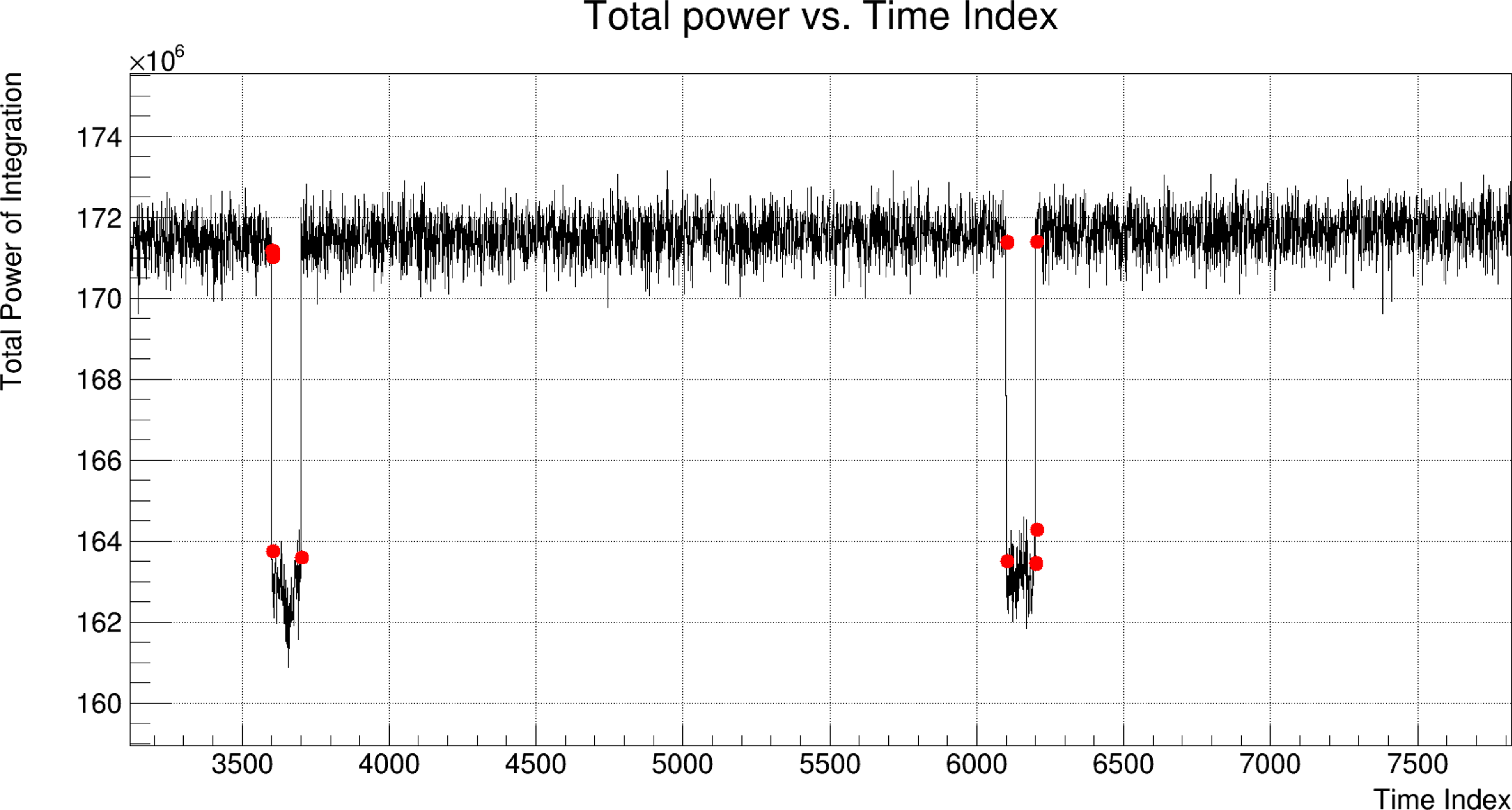
Figure 11. Total power as a function of time sample index from one of the Vela observations (internal MWA ID 1359388216). The black curve is the total power in a single coarse channel (153.6 MHz in this case), and the red dots indicate the drops in total power as automatically detected by our software. A single time step corresponds to 10 ms. Hence, the first drop in power (i.e. loss of packets) occurred during a 1-sblock started 36 s after the start of the observation.
On the other hand, similar power variations were observed in V-FASTR experiment (Wayth et al. Reference Wayth, Brisken, Deller, Majid, Thompson, Tingay and Wagstaff2011) and were resolved on the data processing level by subtracting a running mean of signal power. This removed power jumps in their data and may also be the best way to improve the real-time MWA IC pipeline, as even after further software/hardware improvements there may always be some small residual packet losses, and the FRB/SETI search software should be robust against these situations.
5. Summary and future plans
The commensal pipeline for FRB and SETI searches is currently in early stages of development and can form several beams using a single MWA coarse channel (1.28 MHz). The mechanics of the pipeline was verified, and confirmed to produce filterbank files commensally to ongoing MWA observations. We have also deployed a first version of FRB search pipeline running FREDDA software on these filterbank files. The commensal pipeline was also verified on selected pulsars using dedicated observing time (total 40 h). Mean profiles of pulsars B0950+08 and Vela were detected with maximum SNRs $\approx$
49 and
$\approx$
49 and $\sim$
17, respectively. However, single pulses were unequivocally identified only in several observations of the pulsar PSR B0950+08 (maximum SNR
$\sim$
17, respectively. However, single pulses were unequivocally identified only in several observations of the pulsar PSR B0950+08 (maximum SNR $\approx$
17). These results mostly agree with the expectations (Table 4). Especially, that some of the pulsars (e.g. J0837+0610 or PSR B0531+21), which in principle should (at least occasionally) have sufficiently bright single pulses to be detected by the pipeline, could only be observed during daytime making their detections highly unlikely. These objects will be re-observed during nighttime and possibly with larger observing bandwidth. Another possible reason for the non-detections may be a few bad tiles, which are not excluded from the incoherent beam (i.e. sum), contribute noise and possibly RFI, and make detections of fainter pulsars impossible. The exclusion of flagged tiles will be included in the next version of the code.
$\approx$
17). These results mostly agree with the expectations (Table 4). Especially, that some of the pulsars (e.g. J0837+0610 or PSR B0531+21), which in principle should (at least occasionally) have sufficiently bright single pulses to be detected by the pipeline, could only be observed during daytime making their detections highly unlikely. These objects will be re-observed during nighttime and possibly with larger observing bandwidth. Another possible reason for the non-detections may be a few bad tiles, which are not excluded from the incoherent beam (i.e. sum), contribute noise and possibly RFI, and make detections of fainter pulsars impossible. The exclusion of flagged tiles will be included in the next version of the code.
The results of the presented tests show that FREDDA software can be successfully applied to the incoherent MWA beam as it was able to identify most of the pulses from PSR B0950+08. Using one of the datasets with multiple bright pulses, it was verified that $\approx$
85% of them were identified by FREDDA. So, far we were not able to detect single pulses from higher DM objects, but this will become possible once the observing bandwidth is increased. The system is currently being upgraded with additional computers, which should enable capturing and processing of a few coarse channels (up to 10 corresponding to 12.8 MHz bandwidth) leading to an increase in the sensitivity of the FRB search by a factor of
$\approx$
85% of them were identified by FREDDA. So, far we were not able to detect single pulses from higher DM objects, but this will become possible once the observing bandwidth is increased. The system is currently being upgraded with additional computers, which should enable capturing and processing of a few coarse channels (up to 10 corresponding to 12.8 MHz bandwidth) leading to an increase in the sensitivity of the FRB search by a factor of $\approx$
3. The main source of false-positive candidates identified by FREDDA were the abrupt changes in total power, which will be improved by reducing the number of lost packets (ongoing software work) and/or by more robust data processing (e.g. subtraction of running mean). Moreover, addition of an automatic candidate classification is also planned in the near future.
$\approx$
3. The main source of false-positive candidates identified by FREDDA were the abrupt changes in total power, which will be improved by reducing the number of lost packets (ongoing software work) and/or by more robust data processing (e.g. subtraction of running mean). Moreover, addition of an automatic candidate classification is also planned in the near future.
Verification of commensal coherent beamforming functionality is another short term goal, which will enable recording of tied-array beams on several objects within the MWA primary beam. It will speed-up processing of MWA high-time resolution data enabling routine pulsar timing observations, and monitoring of known repeating FRBs. Furthermore, it will also significantly reduce the storage requirements as tied-array beam for a single object requires $N_{ant}$
(128 or 256) less disc space than the full MWA VCS data product. The presented commensal pipeline is routinely running during most of the MWA observations, and once the frequency bandwidth is increased may be able to detect a several bright FRBs per year.
$N_{ant}$
(128 or 256) less disc space than the full MWA VCS data product. The presented commensal pipeline is routinely running during most of the MWA observations, and once the frequency bandwidth is increased may be able to detect a several bright FRBs per year.
Acknowledgements
This scientific work uses data obtained from Inyarrimanha Ilgari Bundara/the MRO. We acknowledge the Wajarri Yamaji People as the Traditional Owners and native title holders of the Observatory site. Support for the operation of the MWA is provided by the Australian Government (NCRIS), under a contract to Curtin University administered by Astronomy Australia Limited. We acknowledge the Pawsey Supercomputing Centre which is supported by the Western Australian and Australian Governments. Inyarrimanha Ilgari Bundara, the CSIRO Murchison Radio-astronomy Observatory and the Pawsey Supercomputing Research Centre are initiatives of the Australian Government, with support from the Government of Western Australia and the Science and Industry Endowment Fund. This research has made use of NASA’s Astrophysics Data System.
Data Availability
Not applicable.
Appendix A
The flux density of a pulsar can be estimated from folded profile created by pulsar processing software such as PRESTO or DSPSR, and SEFD calculated using beam model of an MWA tile or an SKA-Low station (Sokolowski et al. Reference Sokolowski2022b). This approach was successfully applied to SKA-Low prototype stations data to measure flux densities of selected pulsars as described by Lee et al. (Reference Lee, Bhat, Sokolowski, Swainston, Ung, Magro and Chiello2022). In this paper, we used the same method to measure mean flux density of Vela pulsar in data from the Aperture Verification System 2 (AAVS2), and we also applied similar procedure using MWA FEE beam model (Sokolowski et al. Reference Sokolowski2017) to the MWA data recorded for the work presented here. Vela profile is highly scattered at low frequencies (example in Fig. A1), and it is often difficult to find a suitable window within the pulse period when the pulsar emission is not present and observed standard deviation ( $\sigma_o$
) of the noise can be calculated. However, either the phase bins before the on-set of the pulse can be used, or a mathematical representation of the pulse profile can be fitted, subtracted and
$\sigma_o$
) of the noise can be calculated. However, either the phase bins before the on-set of the pulse can be used, or a mathematical representation of the pulse profile can be fitted, subtracted and $\sigma_o$
can be measured as the standard deviation of the residuals. We used both these approaches and they led to nearly identical results. In a short summary mean flux and peak flux densities of Vela pulsar and other pulsars in our test sample were calculated according to the following procedure:
$\sigma_o$
can be measured as the standard deviation of the residuals. We used both these approaches and they led to nearly identical results. In a short summary mean flux and peak flux densities of Vela pulsar and other pulsars in our test sample were calculated according to the following procedure:

Figure A1. Example fit of equation (A1) to 2013-06-14 MWA data at 216 MHz, which enabled calculation of the mean flux m $\approx$
7.8 Jy and peak flux
$\approx$
7.8 Jy and peak flux $\approx$
31 Jy, and estimation of W10
$\approx$
31 Jy, and estimation of W10 $\approx$
50 ms as the time width of the pulse where the flux density is
$\approx$
50 ms as the time width of the pulse where the flux density is $\ge$
10% of the peak value (summarised in Table 4).
$\ge$
10% of the peak value (summarised in Table 4).
-
1. Calculate observed standard deviation of the noise (
$\sigma_o$
) from the off-pulse part of the folded profile (e.g. phase window 0.8–1.0 in Fig. A1) or from the residuals after subtracting the fitted mathematical representation of the mean profile. -
2. Divide average pulse profile by
$\sigma_o$
in order to re-scale uncalibrated flux density such that new standard deviation is 1. Divide values on X-axis by their maximum value (typically number of bins
$n_{bin}$
if it was originally bin index) in order to re-scale X-axis to [0,1] range. -
3. Fit a mathematical function to the mean pulse profile. We found that the best fit resulted from a sum of a Gaussian function (representing the on-set and peak of the pulse) multiplied by exponential decay (only for phase values higher than phase of the peak flux). This can be mathematically described as:
(A1)where G(p) is the Gaussian profile used to describe the pulse peak:
\begin{equation}f(p) =\begin{cases} G(p)\text{ for p }\le p_{peak} \\[5pt] G(p) \cdot e^{-\frac{(p-p_{peak})}{\tau}} \text{ for p }\ge p_{peak} \\\end{cases}\end{equation}
(A2)and p is the phase of the average pulse period in [0,1] range,
\begin{equation}G(p) = \frac{f_p}{\sqrt{2\pi \sigma_p}} \cdot e^{-\frac{(p-p_{peak})^2}{2\sigma_p^2}},\end{equation}
$\sigma_p$
is standard deviation of the Gaussian profile,
$p_{peak}$
is the phase corresponding to peak flux density,
$\tau$
corresponds to scattering time in units of pulsar phase (hence unitless here) and
$f_p$
is the peak flux density of the average profile. Example of fitted profile is shown in Fig. A1. Simpler pulse profiles (e.g. for pulsar B0950+08) were fitted with a Gaussian profile (G(p)) only, that is, without the exponential tail term.
-
4. Calculate expected standard deviation of the noise (
$\sigma_s$
) in the incoherent sum of all MWA tiles, using
$\text{SEFD}_X$
and
$\text{SEFD}_Y$
calculated with the MWA FEE Beam model (Sokolowski et al. Reference Sokolowski2017) and the following equation:(A3)where
\begin{equation}\sigma_s = \frac{\text{SEFD}_I\sqrt{n_{bin}}}{\sqrt{\Delta \nu T}}\end{equation}
$n_{bin}$
is the number of phase bins in the average pulse profile,
$\Delta \nu$
is the observing bandwidth, T is total integration time of typically 290 s (thus the integration time per phase bin of the pulse profile is
$\Delta t = T / n_{bin}$
), and
$\text{SEFD}_I$
is Stokes I polarisation calculated from
$\text{SEFD}_X$
and
$\text{SEFD}_Y$
according to equation 3.
-
5. Calculate calibration coefficient
$z = \frac{\sigma_s}{\sigma_o}$
, and use it to calculate calibrated flux density in each phase bin i according to:
$f_c^i = z \cdot f_u^i$
, where
$f_u^i$
and
$f_c^i$
are, respectively, uncalibrated and calibrated flux densities in the phase bin i. -
6. Calculate calibrated mean flux density as:
(A4)where F is fluence and P pulsar period.
\begin{equation}m = \frac{F}{P} = \frac{\text{SEFD}_I \times \sum_{i=0}^{n_{bin}} f_u^{i}}{\sigma_o \sqrt{\Delta \nu \cdot T \cdot n_{bin}}},\end{equation}
-
7. Calculate calibrated peak flux
$f_p$
as:(A5)
\begin{equation}f_p = \max\limits_{1\leq i\leq n_{bin}} [ f_c^{i} ]\end{equation}


 Open access