


1. Introduction
Since the first high redshift ( $z \gtrsim 3$
) survey for cold neutral (star-forming) gas, via the absorption of the 21-cm transition of neutral hydrogen in the host galaxies of distant radio sources, it has been posited that the dearth of detections is due to the selection of ultraviolet (UV) luminous sources. In these objects, the UV radiation from the active galactic nucleus (AGN) is sufficient to ionise the gas to below the detection limits of large radio telescopes (Curran et al. Reference Curran, Whiting, Wiklind, Webb, Murphy and Purcell2008b
). While a steady decrease with redshift, and hence UV luminosity, may be expected, an abrupt cut-off in the detection of H i above
$z \gtrsim 3$
) survey for cold neutral (star-forming) gas, via the absorption of the 21-cm transition of neutral hydrogen in the host galaxies of distant radio sources, it has been posited that the dearth of detections is due to the selection of ultraviolet (UV) luminous sources. In these objects, the UV radiation from the active galactic nucleus (AGN) is sufficient to ionise the gas to below the detection limits of large radio telescopes (Curran et al. Reference Curran, Whiting, Wiklind, Webb, Murphy and Purcell2008b
). While a steady decrease with redshift, and hence UV luminosity, may be expected, an abrupt cut-off in the detection of H i above $L_\textrm{UV} \sim10^{23}$
W Hz
$L_\textrm{UV} \sim10^{23}$
W Hz $^{-1}$
(ionising photon rates of
$^{-1}$
(ionising photon rates of $Q_{{\textrm{H}\,\scriptsize{\textrm{I}}}}\gtrsim 10^{56}$
s
$Q_{{\textrm{H}\,\scriptsize{\textrm{I}}}}\gtrsim 10^{56}$
s $^{-1}$
) is apparent. Curran & Whiting (Reference Curran and Whiting2012) showed that such a critical luminosity would arise from an exponential gas distribution, with the observed value being close that required to ionise all of the gas in the Milky Way, that is, a large spiral.
$^{-1}$
) is apparent. Curran & Whiting (Reference Curran and Whiting2012) showed that such a critical luminosity would arise from an exponential gas distribution, with the observed value being close that required to ionise all of the gas in the Milky Way, that is, a large spiral.
Since then, this observational result has been confirmed, not only over specific ‘homogeneous’ subsets of sources (compact, extended, flat spectrum, etc., Curran et al. Reference Curran, Whiting, Tanna, Sadler, Pracy and Athreya2013b , Reference Curran, Allison, Whiting, Sadler, Combes, Pracy, Bignell and Athreya2016; Aditya, Kanekar, & Kurapati Reference Aditya, Kanekar and Kurapati2016; Aditya & Kanekar Reference Aditya and Kanekar2018a ; Grasha et al. Reference Grasha, Darling and Bolatto2019; Murthy et al. Reference Murthy, Morganti, Oosterloo and Maccagni2021, Reference Murthy, Morganti, Kanekar and Oosterloo2022), but also unbiased samples, limited only by flux (Curran et al. Reference Curran2011, Reference Curran, Whiting, Sadler and Bignell2013a, Reference Curran, Whiting, Allison, Tanna, Sadler and Athreya2017a, Reference Curran, Hunstead, Johnston, Whiting, Sadler, Allison and Bignellb, Reference Curran, Hunstead, Johnston, Whiting, Sadler, Allison and Athreya2019; Allison et al. Reference Allison2012; Geréb et al. Reference Geréb, Maccagni, Morganti and Oosterloo2015). The complete ionisation of the gas within the host galaxies of these objects would prevent star formation within them and is strongly indicative of a selection effect, where the traditional need for a reliable optical redshift, to which to tune the radio band receiver, causes a bias towards the most UV luminous sources (Curran et al. Reference Curran, Whiting, Wiklind, Webb, Murphy and Purcell2008b ). This suggests a population of undetected gas-rich galaxies in the distant Universe, too faint to be detected via optical spectroscopy.
There is, however, still some debate over this interpretation: Curran et al. (Reference Curran, Whiting, Wiklind, Webb, Murphy and Purcell2008b ) also noted that all of the sources above the critical UV luminosity were type 1 objects (quasars), suggesting that the gas could be undetected due to the obscuring circum-nuclear torus, invoked by unified schemes of AGN (Osterbrock Reference Osterbrock1978; Antonucci & Miller Reference Antonucci and Miller1985; Miller & Goodrich Reference Miller and Goodrich1987), not intercepting our sight-line to the AGN. However, below the critical UV luminosity the detection rate was similar to that in type-2 objects (galaxies), suggesting that the bulk of the absorption occurs in the large-scale galactic disk, which is randomly orientated to the pc-scale torus (Curran & Whiting Reference Curran and Whiting2010). Furthermore, rather than photo-ionisation from the AGN being the dominant cause of the decrease in detection rate with redshift, Aditya & Kanekar (Reference Aditya and Kanekar2018a, Reference Aditya and Kanekar b ), Aditya et al. (Reference Aditya2024) propose excitation of the hydrogen by 1.4 GHz photons (Purcell & Field Reference Purcell and Field1956; Field Reference Field1959) or some other (unspecified) evolutionary effect. While the former has been ruled out (Curran et al. Reference Curran, Whiting, Wiklind, Webb, Murphy and Purcell2008b , Reference Curran, Hunstead, Johnston, Whiting, Sadler, Allison and Athreya2019, see also Section 3.1.3), the latter effects would have to apply across the whole sample, irrespective of source classification in order to usurp the ionisation hypothesis.
Most recently, there have been five detections of H i absorption (Chowdhury, Kanekar, & Chengalur Reference Chowdhury, Kanekar and Chengalur2020; Murthy et al. Reference Murthy, Morganti, Oosterloo and Maccagni2021; Su et al. Reference Su2022; Aditya et al. Reference Aditya2024), where the column density would exceed the theoretical limit of $N_{{{\textrm{H}\,\scriptsize{\textrm{I}}}}}\sim 10^{22}$ $\textrm{cm}^{-2}$
(Schaye Reference Schaye2001), for moderate spin temperatures. In this paper, we reassess the ionisation hypothesis in light of these and the vastly increased sample of published H i searches.
$\textrm{cm}^{-2}$
(Schaye Reference Schaye2001), for moderate spin temperatures. In this paper, we reassess the ionisation hypothesis in light of these and the vastly increased sample of published H i searches.
2. Analysis
2.1. The data
Adding the recent searches, comprising 441 objects (Chowdhury et al. Reference Chowdhury, Kanekar and Chengalur2020; Murthy et al. Reference Murthy, Morganti, Oosterloo and Maccagni2021, Reference Murthy, Morganti, Kanekar and Oosterloo2022; Mahony et al. Reference Mahony2022; Su et al. Reference Su2022; Aditya et al. Reference Aditya2024; Deka et al. Reference Deka2024), to those compiled in Curran et al. (Reference Curran, Hunstead, Johnston, Whiting, Sadler, Allison and Athreya2019) there are now 924 $z\geq0.1$
sources in the literature which have been searched for associated H i 21-cm absorption. These are made up of 100 detections and 824 non-detections.
$z\geq0.1$
sources in the literature which have been searched for associated H i 21-cm absorption. These are made up of 100 detections and 824 non-detections.
2.2. Photometry and fitting
To obtain the ionising photon rate for each of the 924 sources, their photometry were scraped from the NASA/IPAC Extragalactic Database (NED), the Wide-Field Infrared Survey Explorer (WISE, Wright et al. Reference Wright2010), Two Micron All Sky Survey (2MASS, Skrutskie et al. Reference Skrutskie2006), and the Galaxy Evolution Explorer (GALEX, data release GR6/7)Footnote a databases. After shifting the data back into the source’s rest-frame, each flux density measurement, $S_{\nu}$
, was then converted to a specific luminosity, via
$S_{\nu}$
, was then converted to a specific luminosity, via $L_{\nu}=4\pi \, D_\textrm{L}^2 \,S_{\nu}/(z+1)$
, where
$L_{\nu}=4\pi \, D_\textrm{L}^2 \,S_{\nu}/(z+1)$
, where $D_\textrm{L}$
is the luminosity distance to the source (see Fig. 1).Footnote b To obtain the ionising photon rate, we use (Osterbrock Reference Osterbrock1989):
$D_\textrm{L}$
is the luminosity distance to the source (see Fig. 1).Footnote b To obtain the ionising photon rate, we use (Osterbrock Reference Osterbrock1989):
 \begin{equation}Q_{{\textrm{H}\,\scriptsize{\textrm{I}}}}\equiv\int^{\infty}_{\nu_\textrm{ion}}\frac{L_{\nu}}{h\nu}\,d{\nu},\end{equation}
where $\nu$
is the frequency (with
$\nu$
is the frequency (with $\nu_\textrm{ion} = 3.29\times10^{15}$
Hz for H i) and h the Planck constant. Fitting the rest-frame UV data with a power-law fit,
$\nu_\textrm{ion} = 3.29\times10^{15}$
Hz for H i) and h the Planck constant. Fitting the rest-frame UV data with a power-law fit, $L_{\nu} \propto \nu^{\alpha}$
, gives
$L_{\nu} \propto \nu^{\alpha}$
, gives
 \begin{equation}\log_{10}L_{\nu} = \alpha\log_{10}\nu+ {C},\end{equation}
where C is the log-space intercept and $\alpha$
the gradient (the spectral index). Integrating this over
$\alpha$
the gradient (the spectral index). Integrating this over $\nu_\textrm{ion}$
to
$\nu_\textrm{ion}$
to $\infty$
gives the ionising photon rate as:
$\infty$
gives the ionising photon rate as:
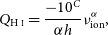 \begin{equation}Q_{{\textrm{H}\,\scriptsize{\textrm{I}}}} = \frac{-10^{C}}{\alpha h}\nu_\textrm{ion}^{\alpha},\end{equation}
shown by the shaded region in Fig. 1. In order to ensure a sufficient sample size, while not contaminating the UV with optical band data, we fit all photometry with $\log_{10}\nu \geq 15.1$
(shown by the dotted line in the figure), which left 180 sources with sufficient UV data. Of these, 19 have been detected in H i.
$\log_{10}\nu \geq 15.1$
(shown by the dotted line in the figure), which left 180 sources with sufficient UV data. Of these, 19 have been detected in H i.
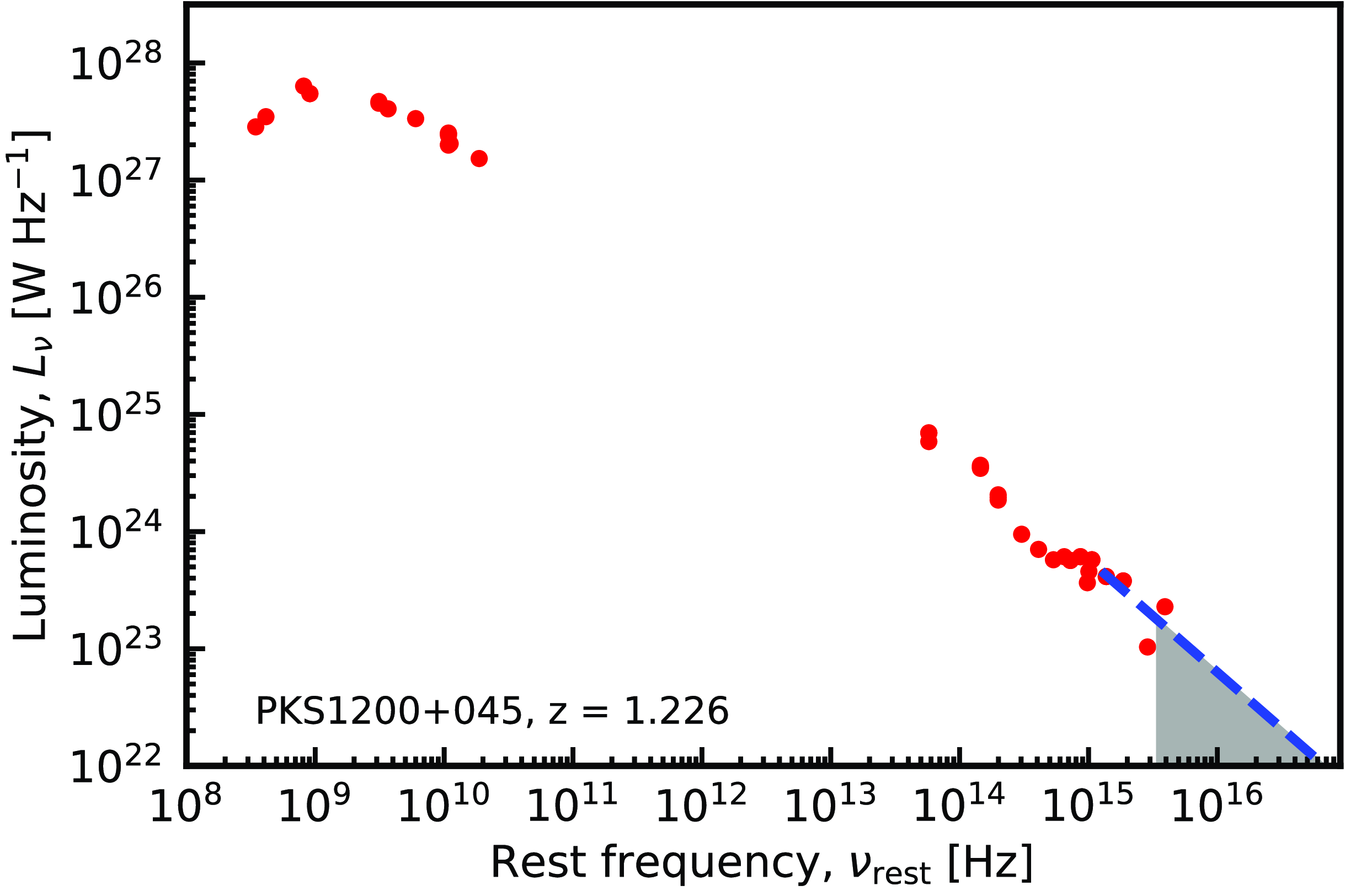
Figure 1. Example of the rest-frame photometry. The dotted line shows the power-law fit to the UV data and the shaded region $\nu \geq 3.29\times10^{15}$
Hz over which the ionising photon rate is calculated. Here, we show PKS 1200+045, which with
$\nu \geq 3.29\times10^{15}$
Hz over which the ionising photon rate is calculated. Here, we show PKS 1200+045, which with $Q_{{\textrm{H}\,\scriptsize{\textrm{I}}}} = 2.9\times10^{56}$
s
$Q_{{\textrm{H}\,\scriptsize{\textrm{I}}}} = 2.9\times10^{56}$
s $^{-1}$
is the highest ionising photon rate at which H i absorption has been detected (see Section 3.3).
$^{-1}$
is the highest ionising photon rate at which H i absorption has been detected (see Section 3.3).
2.3. H i absorption strength
The strength of the H i 21-cm absorption is given by the profile’s velocity-integrated optical depth ( $\int\!\tau\,dv$
), which is analogous to the equivalent width in optical-band spectroscopy. This is related to the total neutral hydrogen column density via
$\int\!\tau\,dv$
), which is analogous to the equivalent width in optical-band spectroscopy. This is related to the total neutral hydrogen column density via
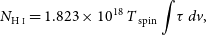 \begin{equation}N_{{{\textrm{H}\,\scriptsize{\textrm{I}}}}} =1.823\times10^{18}\,T_\textrm{ spin}\int\!\tau\,dv,\end{equation}
where the spin temperature, $T_\textrm{spin}$
, quantifies the excitation from the lower hyperfine level of the hydrogen atom (Purcell & Field Reference Purcell and Field1956).
$T_\textrm{spin}$
, quantifies the excitation from the lower hyperfine level of the hydrogen atom (Purcell & Field Reference Purcell and Field1956).
We do not measure the intrinsic optical depth directly, but rather the observed optical depth, $\tau_\textrm{obs}$
, which is the ratio of the line depth,
$\tau_\textrm{obs}$
, which is the ratio of the line depth, $\Delta S$
, to the observed background flux,
$\Delta S$
, to the observed background flux, $S_\textrm{obs}$
. The two are related via
$S_\textrm{obs}$
. The two are related via
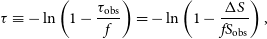 \begin{equation}\tau \equiv-\ln\left(1-\frac{\tau_\textrm{obs}}{f}\right) = -\ln\left(1-\frac{\Delta S}{fS_\textrm{obs}}\right),\end{equation}
where the covering factor, f, is the fraction of $S_\textrm{obs}$
intercepted by the absorber. In the optically thin regime, where
$S_\textrm{obs}$
intercepted by the absorber. In the optically thin regime, where $\tau_\textrm{obs} \lesssim 0.3$
,
$\tau_\textrm{obs} \lesssim 0.3$
, $\tau \approx \tau_\textrm{obs}/f$
, so that Equation (4) can be approximated as:
$\tau \approx \tau_\textrm{obs}/f$
, so that Equation (4) can be approximated as:
 \begin{equation} N_{{{\textrm{H}\,\scriptsize{\textrm{I}}}}} \approx 1.823\times10^{18}\,\frac{T_\textrm{ spin}}{f}\int\!\tau_\textrm{obs}\,dv.\end{equation}
For the non-detections, the upper limit to the line strength is obtained via $ \tau_\textrm{obs} = {3\sigma_\textrm{rms}}/S_\textrm{obs}$
, where
$ \tau_\textrm{obs} = {3\sigma_\textrm{rms}}/S_\textrm{obs}$
, where $\sigma_\textrm{rms}$
is the rms noise level of the spectrum. In order to place each of the limits on an equal, footing each is re-sampled to the same spectral resolution (
$\sigma_\textrm{rms}$
is the rms noise level of the spectrum. In order to place each of the limits on an equal, footing each is re-sampled to the same spectral resolution ( $\Delta v = 20$ $\textrm{km s}^{-1}$
), which is then used as the full-width at half maximum to obtain the integrated optical depth limit per channel (see Curran Reference Curran2012).
$\textrm{km s}^{-1}$
), which is then used as the full-width at half maximum to obtain the integrated optical depth limit per channel (see Curran Reference Curran2012).
Common practice is to convert the observed velocity integrated optical depth to a column density, by assuming the spin temperature (and, presumably, $f=1$
, e.g. Su et al. Reference Su2023). However, since we have no information on this, or the covering factor,Footnote c we define the normalised line strength:
$f=1$
, e.g. Su et al. Reference Su2023). However, since we have no information on this, or the covering factor,Footnote c we define the normalised line strength:
 \begin{equation}1.823\times10^{18}\,\int\!\tau_\textrm{obs}\,dv, \textrm{which gives } N_{{{\textrm{H}\,\scriptsize{\textrm{I}}}}}\left(\frac{f}{T_\textrm{ spin}}\right).\end{equation}
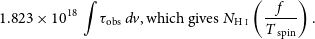
Showing the distributions in Fig. 2, we see that while, in general, the non-detections have been searched sufficiently deeply to detect H i absorption, the sample of Su et al. (Reference Su2022) may not have been.Footnote d In order to reduce any bias by including weaker limits, in the rest of the analysis we only consider non-detections searched to $N_{{{\textrm{H}\,\scriptsize{\textrm{I}}}}}\leq 10^{19}\,(T_\textrm{spin}/f)$ $\textrm{cm}^{-2}$
.
$\textrm{cm}^{-2}$
.
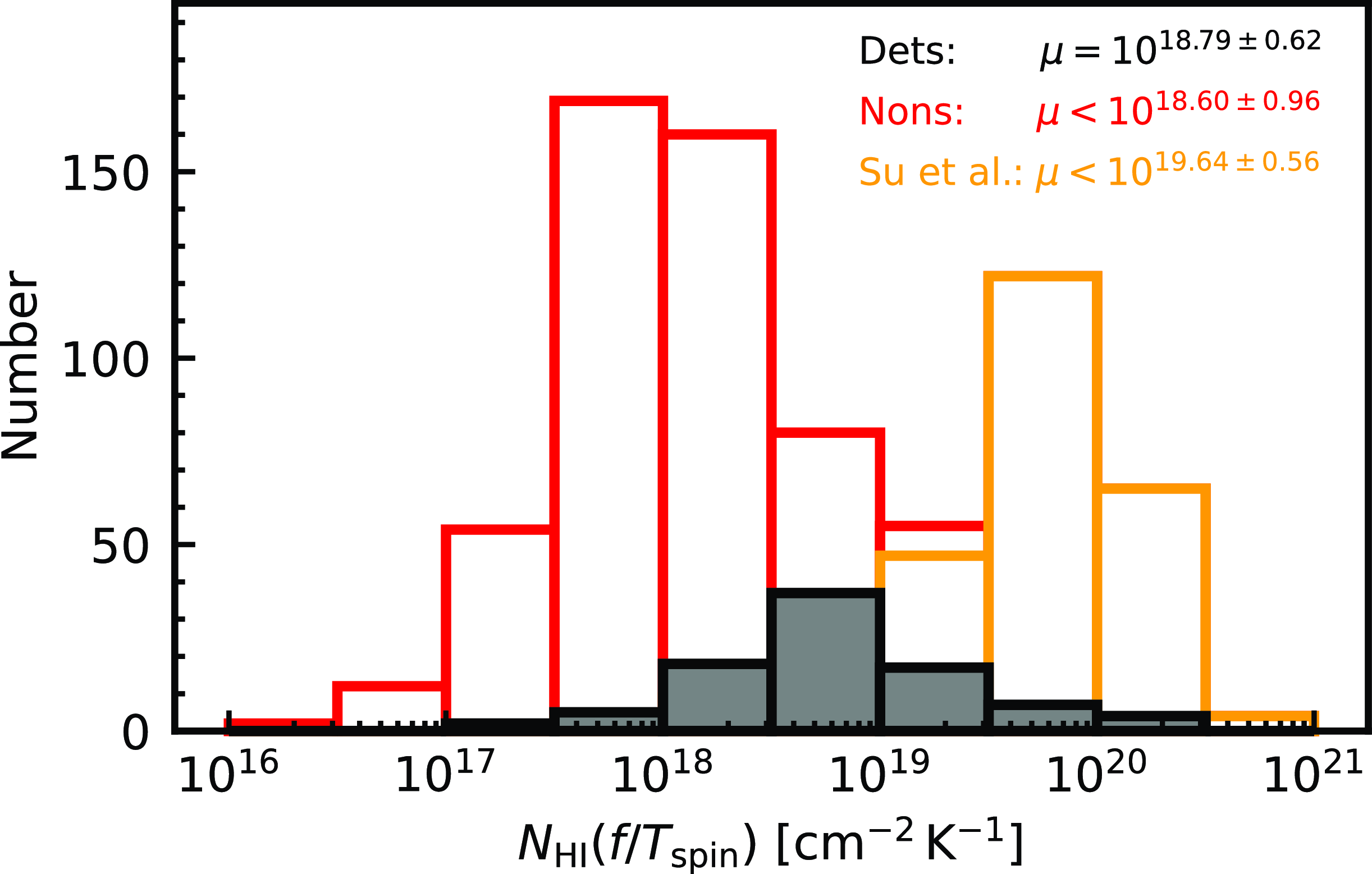
Figure 2. The distributions of the normalised line strengths for the detections (filled histogram) and the upper limits (unfilled), which have been separated into the upper limits of Su et al. (Reference Su2022) and the rest of the sample. The legend shows the mean ( $\pm1\sigma$
) value of each distribution.
$\pm1\sigma$
) value of each distribution.
3. Results and discussion
3.1. Factors affecting the detection of H i
3.1.1. Source classification
In Fig. 3, we show the derived ionising photon rates versus the look-back time/redshift. At low redshifts, we can see the high detection rate reported previously (e.g. Vermeulen et al. Reference Vermeulen2003; Maccagni et al. Reference Maccagni, Morganti, Oosterloo, Geréb and Maddox2017). At best, we would expect a $\approx50$
% rate from the random orientation of the absorbing medium, whether this be in the obscuring torus or the large-scale galactic disk. However, it is clear that there is a sharp decrease in the detection rate with redshift, which may be caused by the preferential selection of type 1 objects (quasars), where the AGN is not obscured by the torus.
$\approx50$
% rate from the random orientation of the absorbing medium, whether this be in the obscuring torus or the large-scale galactic disk. However, it is clear that there is a sharp decrease in the detection rate with redshift, which may be caused by the preferential selection of type 1 objects (quasars), where the AGN is not obscured by the torus.
Figure 3. The ionising photon rate versus the look-back time. The filled symbols show the H i detections and the unfilled the non-detections, with the shapes designating the source classification: quasars – stars, galaxies – circles, other – squares. The lower panel shows the H i detection rate at various look-back times, where the error bars on the ordinate show the Poisson standard errors and abscissa the range over which these apply.
The galaxy and quasar detection rates are shown in Fig. 4. Ignoring the 50 and 100% values, which comprise only one or two objects, we see that both detection rates drop with increasing $Q_{{\textrm{H}\,\scriptsize{\textrm{I}}}}$
. This is much steeper for galaxies, although these start from much higher values. Below the critical UV luminosity, Curran et al. (Reference Curran, Whiting, Wiklind, Webb, Murphy and Purcell2008b
) found a
$Q_{{\textrm{H}\,\scriptsize{\textrm{I}}}}$
. This is much steeper for galaxies, although these start from much higher values. Below the critical UV luminosity, Curran et al. (Reference Curran, Whiting, Wiklind, Webb, Murphy and Purcell2008b
) found a $53\pm10$
% detection rate for galaxies and
$53\pm10$
% detection rate for galaxies and $33\pm13$
% for quasars at
$33\pm13$
% for quasars at $L_{\mathrm UV} \lesssim 10^{23}$
W Hz
$L_{\mathrm UV} \lesssim 10^{23}$
W Hz $^{-1}$
. The current numbers are smaller as we use the more stringent
$^{-1}$
. The current numbers are smaller as we use the more stringent $\log_{10}\nu \geq15.1$
, cf.
$\log_{10}\nu \geq15.1$
, cf. $\log_{10}\nu \geq 14.8$
, for the UV data, as well as the ionising photon rate (by integrating the UV photometry), rather than the monochromatic luminosity, which requires more complete UV photometry. If we ignore the small number statistics,Footnote e this suggests that the orientation of the torus may play a role, but given that quasars are nevertheless detected in H i absorption, this cannot be the whole story. Note also that Murthy et al. (Reference Murthy, Morganti, Kanekar and Oosterloo2022) do not detect absorption in any of their 29 targets, considered to be galaxies and therefore expected to yield several detections. However, the choice of targeting extended objects may bias towards lowering covering factors, the effect of which is suspected of reducing the observed optical depth in extended radio sources (Curran et al. Reference Curran, Allison, Glowacki, Whiting and Sadler2013c
).
$\log_{10}\nu \geq 14.8$
, for the UV data, as well as the ionising photon rate (by integrating the UV photometry), rather than the monochromatic luminosity, which requires more complete UV photometry. If we ignore the small number statistics,Footnote e this suggests that the orientation of the torus may play a role, but given that quasars are nevertheless detected in H i absorption, this cannot be the whole story. Note also that Murthy et al. (Reference Murthy, Morganti, Kanekar and Oosterloo2022) do not detect absorption in any of their 29 targets, considered to be galaxies and therefore expected to yield several detections. However, the choice of targeting extended objects may bias towards lowering covering factors, the effect of which is suspected of reducing the observed optical depth in extended radio sources (Curran et al. Reference Curran, Allison, Glowacki, Whiting and Sadler2013c
).
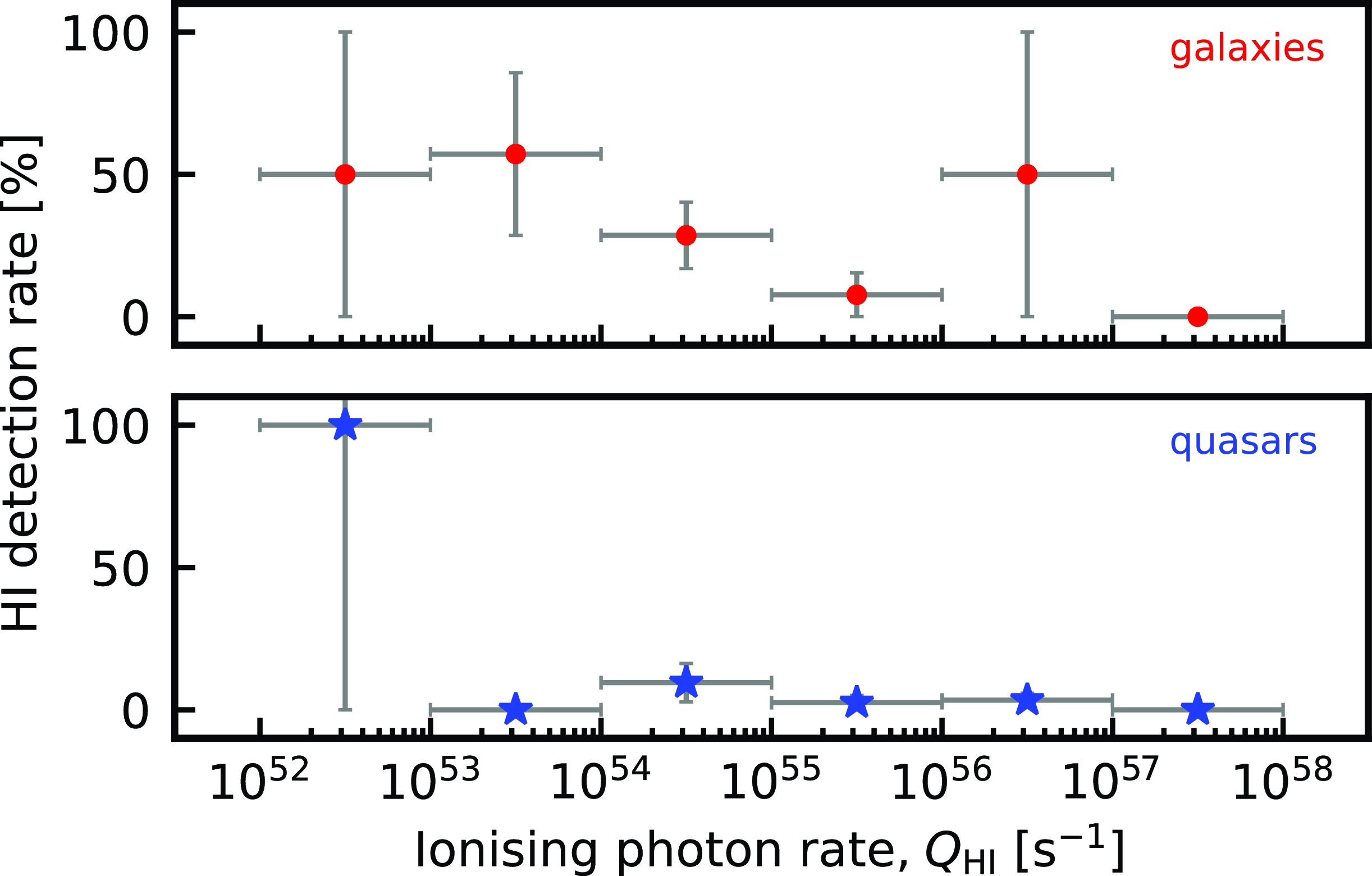
Figure 4. The detection rate versus the ionising photon rate for the galaxies and the quasars. The error bars are as described in Fig. 3. For the galaxies, the exact 50% detection rates are due to a single detection and non-detection in the range and the 100% detection rate for the quasars is due to only having a single object in the range. The H i detected galaxy in the $Q_{{\textrm{H}\,\scriptsize{\textrm{I}}}} = 10^{56} - 10^{57}\textrm{ s}^{-1}$
bin is PKS 1200+045 (see Section 3.3).
$Q_{{\textrm{H}\,\scriptsize{\textrm{I}}}} = 10^{56} - 10^{57}\textrm{ s}^{-1}$
bin is PKS 1200+045 (see Section 3.3).
Lastly, there is the simple explanation that quasars are generally more luminous than galaxies (e.g. Antonucci Reference Antonucci1993) and, by scaling, have correspondingly higher ionisation rates. This is apparent in Fig. 5, where the UV and radio luminosities are strongly correlated [ $p(\tau) = 2.17\times10^{-14}$
]. That is, the Malmquist bias towards brighter objects at high redshift, and fainter objects at low redshift, means that the brighter quasars will be more UV luminous resulting in a lower H i detection rate.
$p(\tau) = 2.17\times10^{-14}$
]. That is, the Malmquist bias towards brighter objects at high redshift, and fainter objects at low redshift, means that the brighter quasars will be more UV luminous resulting in a lower H i detection rate.
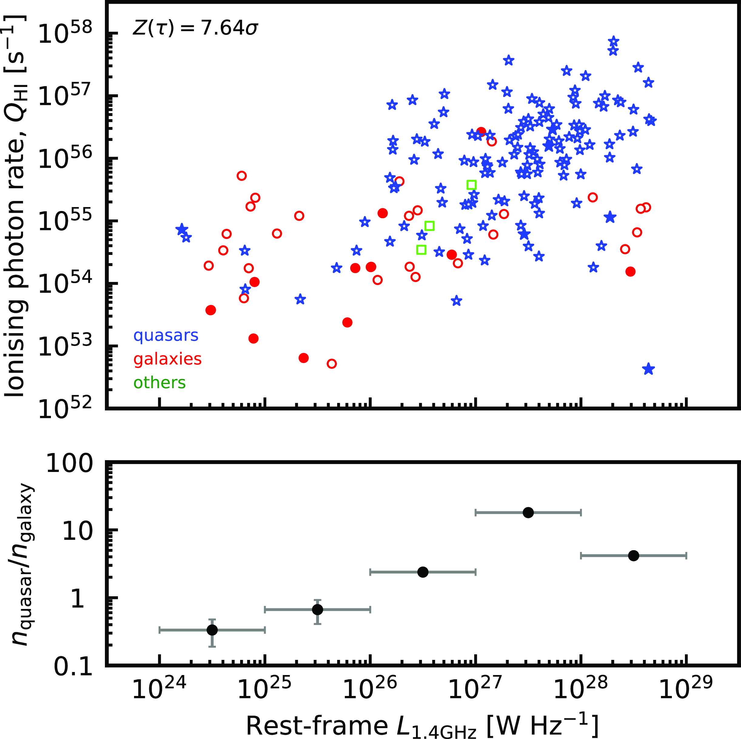
Figure 5. The ionising photon rate versus the 21-cm continuum luminosity. The bottom panel shows the ratio of quasars to galaxies in each $L_{\textrm{1.4 GHz}}$
bin.
$L_{\textrm{1.4 GHz}}$
bin.
3.1.2. Ionising photon rate
In Fig. 6, we show the distribution of the normalised line strengths versus the ionising photon rates for the sources which have sufficient UV photometry. For the 19 detections alone, the Kendall’s tau test gives a probability of $p(\tau) = 0.046$
for the
$p(\tau) = 0.046$
for the $N_{{{\textrm{H}\,\scriptsize{\textrm{I}}}}}/({f}{T_\textrm{spin}})-Q_{{{\textrm{H}\,\scriptsize{\textrm{I}}}}}$
anti-correlation occurring by chance. This is significant at
$N_{{{\textrm{H}\,\scriptsize{\textrm{I}}}}}/({f}{T_\textrm{spin}})-Q_{{{\textrm{H}\,\scriptsize{\textrm{I}}}}}$
anti-correlation occurring by chance. This is significant at $1.99\sigma$
, assuming Gaussian statistics. If we include the upper limits, as censored data points, via the Astronomy SURVival Analysis (asurv) package (Isobe, Feigelson, & Nelson Reference Isobe, Feigelson and Nelson1986), the probability becomes
$1.99\sigma$
, assuming Gaussian statistics. If we include the upper limits, as censored data points, via the Astronomy SURVival Analysis (asurv) package (Isobe, Feigelson, & Nelson Reference Isobe, Feigelson and Nelson1986), the probability becomes $p(\tau) = 3.66\times10^{-6}$
(
$p(\tau) = 3.66\times10^{-6}$
( $4.63\sigma$
).
$4.63\sigma$
).
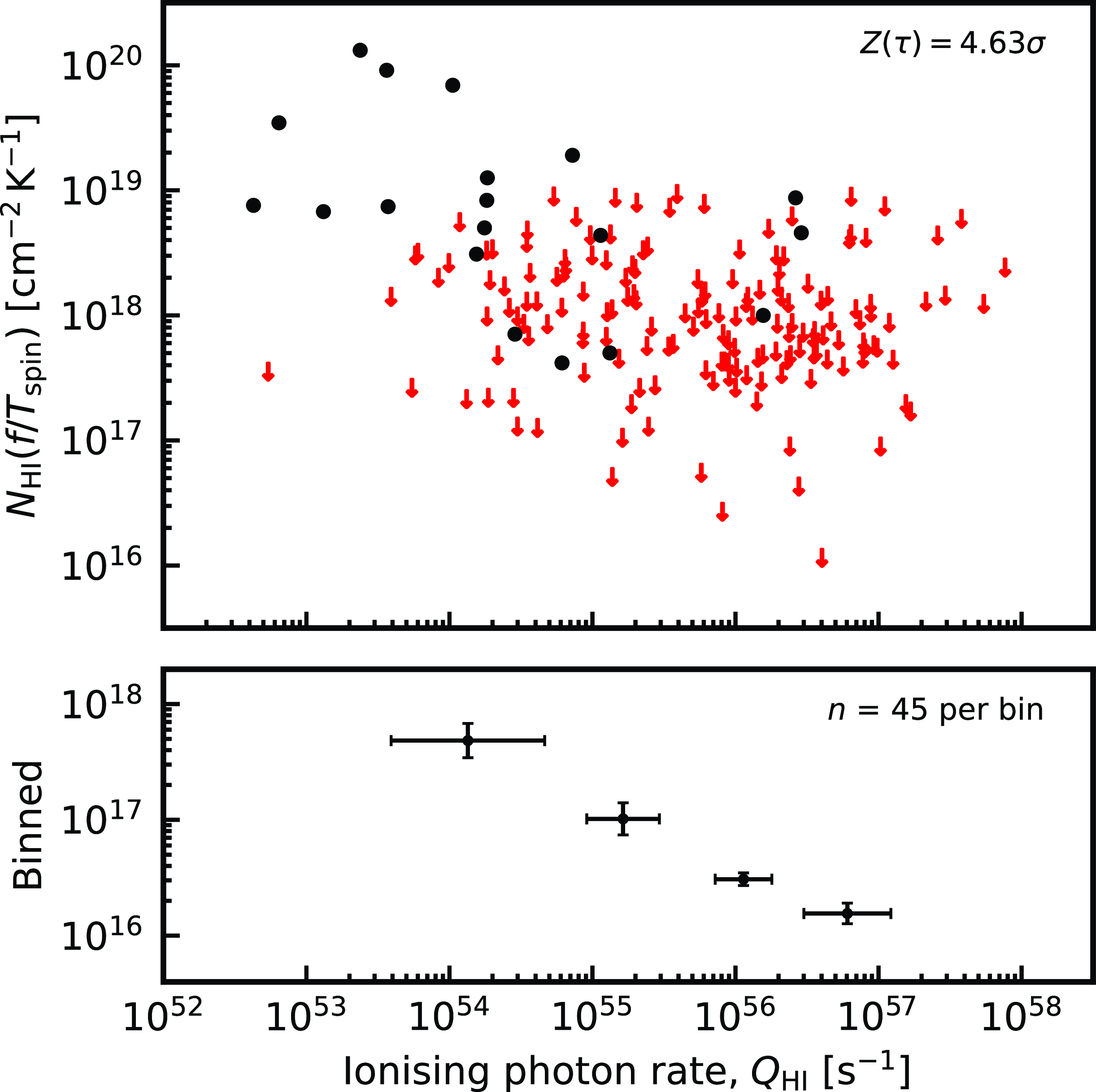
Figure 6. The normalised absorption strength versus the ionising photon rate. The circles show the detections and the arrows the $3\sigma$
upper limits re-sampled to
$3\sigma$
upper limits re-sampled to $\Delta v =$ $20\;\textrm{km s}^{-1}$
. The lower panel shows the data in equally sized bins with
$20\;\textrm{km s}^{-1}$
. The lower panel shows the data in equally sized bins with $\pm1\sigma$
error bars.
$\pm1\sigma$
error bars.
Of the five absorbers with $N_{{{\textrm{H}\,\scriptsize{\textrm{I}}}}} \gtrsim 10^{20}\,(T_\textrm{ spin}/f)$ $\textrm{cm}^{-2}$
, only one has sufficient UV photometry to obtain the ionising photon rate (WISEA J145239.38+062738.2). With
$\textrm{cm}^{-2}$
, only one has sufficient UV photometry to obtain the ionising photon rate (WISEA J145239.38+062738.2). With $Q_{{\textrm{H}\,\scriptsize{\textrm{I}}}} = 2.4\times10^{53}$
s
$Q_{{\textrm{H}\,\scriptsize{\textrm{I}}}} = 2.4\times10^{53}$
s $^{-1}$
, this is well below the
$^{-1}$
, this is well below the $Q_{{\textrm{H}\,\scriptsize{\textrm{I}}}}\sim10^{56}$
s
$Q_{{\textrm{H}\,\scriptsize{\textrm{I}}}}\sim10^{56}$
s $^{-1}$
cut off. However, from the binning in Fig. 6, the anti-correlation between absorption strength and ionising photon rate is clear.Footnote f Lastly, below the maximum detected value of
$^{-1}$
cut off. However, from the binning in Fig. 6, the anti-correlation between absorption strength and ionising photon rate is clear.Footnote f Lastly, below the maximum detected value of $Q_{{\textrm{H}\,\scriptsize{\textrm{I}}}} = 2.9\times10^{56}$
s
$Q_{{\textrm{H}\,\scriptsize{\textrm{I}}}} = 2.9\times10^{56}$
s $^{-1}$
there are 19 detections and 124 non-detections, giving a detection rate of 13.3%. Above the maximum detected value, there are 40 non-detections and, of course, 0 detections. For
$^{-1}$
there are 19 detections and 124 non-detections, giving a detection rate of 13.3%. Above the maximum detected value, there are 40 non-detections and, of course, 0 detections. For $p=0.133$
, the binomial probability of obtaining 0 detections out of 40 at
$p=0.133$
, the binomial probability of obtaining 0 detections out of 40 at $Q_{{\textrm{H}\,\scriptsize{\textrm{I}}}} > 2.9\times10^{56}$
s
$Q_{{\textrm{H}\,\scriptsize{\textrm{I}}}} > 2.9\times10^{56}$
s $^{-1}$
is
$^{-1}$
is $3.32\times10^{-3}$
(
$3.32\times10^{-3}$
( $2.94\sigma$
).
$2.94\sigma$
).
Bear in mind that there will be significant noise in these data, due to different source sizes and morphologies (see Section 3.1.4), and the fact that a large fraction of the non-detections will simply not be orientated favourably for us to detect absorption. This would give, at best, a $\approx50$
% detection rate (Section 3.1.1) and if these could be removed, leaving only the ionisation as the factor under consideration, we could see much more significant results.
$\approx50$
% detection rate (Section 3.1.1) and if these could be removed, leaving only the ionisation as the factor under consideration, we could see much more significant results.
3.1.3. Radio luminosity
As stated above, Aditya & Kanekar (Reference Aditya and Kanekar2018a
,Reference Aditya and Kanekar
b
) propose the excitation of the hydrogen by 1.4 GHz photons as a factor in the decrease in detection rate with redshift, although this was ruled out by Curran et al. (Reference Curran, Whiting, Wiklind, Webb, Murphy and Purcell2008b
). Returning to this, in Fig. 7, we see that the H i absorption strength also exhibits an anti-correlation with the 21-cm continuum luminosity, although with $p(\tau) = 0.0020$
this is considerably weaker than for the ionising photon rate. Furthermore, unlike for
$p(\tau) = 0.0020$
this is considerably weaker than for the ionising photon rate. Furthermore, unlike for $Q_{{\textrm{H}\,\scriptsize{\textrm{I}}}}$
, it is seen that the detections and non-detections occupy a very similar range of luminosities. Quantifying this, below the maximum detected value of
$Q_{{\textrm{H}\,\scriptsize{\textrm{I}}}}$
, it is seen that the detections and non-detections occupy a very similar range of luminosities. Quantifying this, below the maximum detected value of $L_{\textrm{1.4 GHz}} = 4.7\times10^{28}$
W Hz
$L_{\textrm{1.4 GHz}} = 4.7\times10^{28}$
W Hz $^{-1}$
there are 85 detections and 437 non-detections, giving a detection rate of 16.3%. Above the maximum detected value, the 6 non-detections therefore give a binomial probability of
$^{-1}$
there are 85 detections and 437 non-detections, giving a detection rate of 16.3%. Above the maximum detected value, the 6 non-detections therefore give a binomial probability of $0.344$
(
$0.344$
( $0.95\sigma$
) of the distribution arising by chance. Thus, unlike the UV luminosity, there is no evidence of a critical radio luminosity, above which H i is not detected (as previously found by Curran et al. Reference Curran, Whiting, Wiklind, Webb, Murphy and Purcell2008b
, Reference Curran, Hunstead, Johnston, Whiting, Sadler, Allison and Athreya2019). We also note that a correlation between the line strength and radio luminosity would be expected just from scaling with the ionising photon rate (see Fig. 5).
$0.95\sigma$
) of the distribution arising by chance. Thus, unlike the UV luminosity, there is no evidence of a critical radio luminosity, above which H i is not detected (as previously found by Curran et al. Reference Curran, Whiting, Wiklind, Webb, Murphy and Purcell2008b
, Reference Curran, Hunstead, Johnston, Whiting, Sadler, Allison and Athreya2019). We also note that a correlation between the line strength and radio luminosity would be expected just from scaling with the ionising photon rate (see Fig. 5).
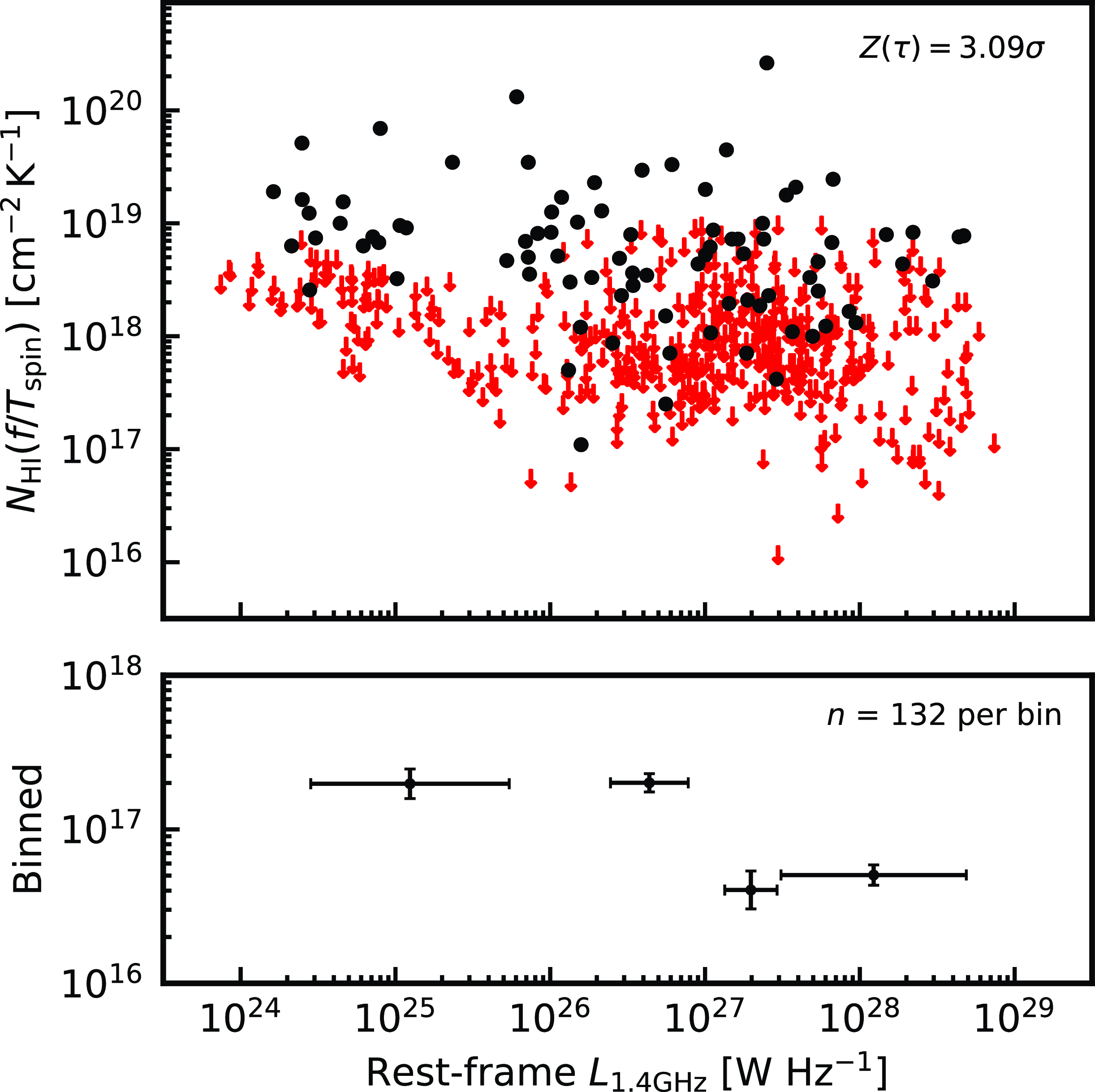
Figure 7. As Fig. 6, but for the 21-cm continuum luminosity.
3.1.4. Other effects
Aditya & Kanekar (Reference Aditya and Kanekar2018a, Reference Aditya and Kanekar b ) and Aditya et al. (Reference Aditya2024) also propose other redshift evolutionary effects as the cause of the decrease in detection rate with redshift. Regarding each of these:
-
− Source morphology: It has long been known that the H i absorption strength is anti-correlated with the size of the source (Pihlström et al. Reference Pihlström, Conway and Vermeulen2003), which Curran et al. Reference Curran, Allison, Glowacki, Whiting and Sadler(2013c ) suggested is a geometry effect introduced by the covering factor, and so we do expect higher detection rates in compact objects. However, given that H i is detected over a range of source sizes, and neither compact nor non-compact objects are detected above the critical UV luminosity (Curran & Whiting Reference Curran and Whiting2010), the ionisation argument remains the more comprehensive.
-
− Gas properties: Evolving gas properties could arise from either a changing column density or evolving spin temperature (see Sections 3.2 & 3.3). Due to the weakness of H i 21-cm emission, we do not usually have a measure of $N_{{{\textrm{H}\,\scriptsize{\textrm{I}}}}}$
at
$z \lesssim 0.1$
, although, from the spectra of damped Lyman-
$\alpha$
absorption systems (DLAs), there is no evidence of any evolution for intervening absorbers (Curran Reference Curran2019 and references therein). Another possibility is an increase in the spin temperature of the gas (cf. the decrease in covering factor above). However, this would be expected to be a result of the high ionisation rates.
$N_{{{\textrm{H}\,\scriptsize{\textrm{I}}}}}$
at
$z \lesssim 0.1$
, although, from the spectra of damped Lyman-
$\alpha$
absorption systems (DLAs), there is no evidence of any evolution for intervening absorbers (Curran Reference Curran2019 and references therein). Another possibility is an increase in the spin temperature of the gas (cf. the decrease in covering factor above). However, this would be expected to be a result of the high ionisation rates. -
− AGN luminosity: Again, this would be a signature of the ionising photon rate, since we have ruled out the effect of the radio luminosity (Section 3.1.3).


Reference Aditya, Jorgenson, Joshi, Singh, An and ChandolaAditya & Kanekar also propose an unspecified evolutionary effect. Due to the Malmquist bias, the ionising photon rate is strongly correlated with the redshift (Fig. 3) and we can test this as above: The maximum redshift at which H i has been detected is $z=3.530$
(Aditya et al. Reference Aditya, Jorgenson, Joshi, Singh, An and Chandola2021). Below this redshift, there are 90 detections and 711 non-detections with
$z=3.530$
(Aditya et al. Reference Aditya, Jorgenson, Joshi, Singh, An and Chandola2021). Below this redshift, there are 90 detections and 711 non-detections with $N_{{{\textrm{H}\,\scriptsize{\textrm{I}}}}}\leq 10^{19}\,(T_\textrm{spin}/f)$ $\textrm{cm}^{-2}$
, giving a detection rate of 11.2%. Thus, the binomial probability of obtaining 0 detections out of 12 at
$\textrm{cm}^{-2}$
, giving a detection rate of 11.2%. Thus, the binomial probability of obtaining 0 detections out of 12 at $z>3.530$
is
$z>3.530$
is $p=0.240$
(
$p=0.240$
( $1.17\sigma$
). That is, the detection of H i appears to be much more dependent on the photo-ionisation than the redshift, although both properties are intimately entwined.
$1.17\sigma$
). That is, the detection of H i appears to be much more dependent on the photo-ionisation than the redshift, although both properties are intimately entwined.
3.2. High column density systems
In Galactic high latitude clouds, above column densities of $N_{{{\textrm{H}\,\scriptsize{\textrm{I}}}}}\approx4\times10^{20}$ $\textrm{cm}^{-2}$
(Reach, Koo, & Heiles Reference Reach, Koo and Heiles1994; Heithausen et al. Reference Heithausen, Brüns, Kerp and Weiss2001)Footnote g the H i begins to form H
$\textrm{cm}^{-2}$
(Reach, Koo, & Heiles Reference Reach, Koo and Heiles1994; Heithausen et al. Reference Heithausen, Brüns, Kerp and Weiss2001)Footnote g the H i begins to form H $_2$
, with Schaye (Reference Schaye2001) suggesting that this is the reason why high redshift absorbers (DLAs) are never found with column densities
$_2$
, with Schaye (Reference Schaye2001) suggesting that this is the reason why high redshift absorbers (DLAs) are never found with column densities $N_{{{\textrm{H}\,\scriptsize{\textrm{I}}}}} \gtrsim 10^{22}$ $\textrm{cm}^{-2}$
. Applying this to the current sample, Curran & Whiting (Reference Curran and Whiting2012) used a simple exponential model of the Galactic gas distribution,
$\textrm{cm}^{-2}$
. Applying this to the current sample, Curran & Whiting (Reference Curran and Whiting2012) used a simple exponential model of the Galactic gas distribution, $n = n(0)e^{-r/R}$
, where R is the scale-length of the decay. Extrapolating from
$n = n(0)e^{-r/R}$
, where R is the scale-length of the decay. Extrapolating from $n = n_0 e^{-(r-R_{\odot})/R}$
, where
$n = n_0 e^{-(r-R_{\odot})/R}$
, where $n_0 = 0.9$ $\textrm{cm}^{-3}$
,
$\textrm{cm}^{-3}$
, $R_{\odot} = 8.5$
kpc and
$R_{\odot} = 8.5$
kpc and $R=3.15$
kpc (Kalberla & Kerp Reference Kalberla and Kerp2009) to
$R=3.15$
kpc (Kalberla & Kerp Reference Kalberla and Kerp2009) to $r=0$
, gave
$r=0$
, gave $n(0)= 13.4$ $\textrm{cm}^{-3}$
. The total column density between the continuum source and ourselves is therefore
$\textrm{cm}^{-3}$
. The total column density between the continuum source and ourselves is therefore
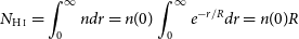 \[N_{{{\textrm{H}\,\scriptsize{\textrm{I}}}}} = \int_0^{\infty} n dr = n(0)\int_0^{\infty}e^{-r/R} dr = n(0)R\] $= 1.3\times10^{23}$ $\textrm{cm}^{-2}$
, which is about an order of magnitude higher than that expected.
$\textrm{cm}^{-2}$
, which is about an order of magnitude higher than that expected.
We therefore proceed by using a compound model, where a constant density component is added over $0\leq r \leq r_0$
to the exponential component (Fig. 8), giving
$0\leq r \leq r_0$
to the exponential component (Fig. 8), giving
 \begin{equation}N_{{{\textrm{H}\,\scriptsize{\textrm{I}}}}} = \int_{0}^{r_0} n_0 dr + \int_{r_0}^{\infty} n_0 e^{-(r-R_{\odot})/R} dr, \end{equation}
where $n_0 = 0.9$ $\textrm{cm}^{-3}$
,
$\textrm{cm}^{-3}$
, $R= 3.15$
kpc,
$R= 3.15$
kpc, $R_{\odot} = 8.5$
kpc and
$R_{\odot} = 8.5$
kpc and $r_0= 7$
kpc (Kalberla & Kerp Reference Kalberla and Kerp2009). To reduce the number of free parameters, we rewrite the formula of Reference Kalberla and KerpKalberla & Kerp:
$r_0= 7$
kpc (Kalberla & Kerp Reference Kalberla and Kerp2009). To reduce the number of free parameters, we rewrite the formula of Reference Kalberla and KerpKalberla & Kerp:
 \[n = n_0 e^{-(r-R_{\odot})/R} \textrm{ as } n = n_0 e^{-(r-r_0)/R},\]
where $n=0$
is now the gas density at
$n=0$
is now the gas density at $r_0$
, e.g.
$r_0$
, e.g. $n_0 = 1.45$ $\textrm{cm}^{-3}$
at
$\textrm{cm}^{-3}$
at $r_0 = 7$
kpc, cf.
$r_0 = 7$
kpc, cf. $n_0 = 0.9$ $\textrm{cm}^{-3}$
at
$\textrm{cm}^{-3}$
at $R_{\odot} = 8.5$
kpc for the Milky Way (Fig. 8). Making the substitution and integrating, Equation (8) becomes
$R_{\odot} = 8.5$
kpc for the Milky Way (Fig. 8). Making the substitution and integrating, Equation (8) becomes
 \begin{equation}N_{{{\textrm{H}\,\scriptsize{\textrm{I}}}}} = n_0\left(r_0 + Re^{-r_0/R}\right),\end{equation}
giving $N_{{{\textrm{H}\,\scriptsize{\textrm{I}}}}}= 3.3\times10^{22}$ $\textrm{cm}^{-2}$
, which is closer to the expected limit.
$\textrm{cm}^{-2}$
, which is closer to the expected limit.
Figure 8. The gas density versus the galactocentric radius for the simple exponential (grey) and compound (red) models of the Milky Way. $r_0$
is radius at which the break between the models occurs.
$r_0$
is radius at which the break between the models occurs.
Since this value is obtained through an inclined disc, we may expect it to be close to representing the theoretical limit. For the five H i absorbers with $N_{{{\textrm{H}\,\scriptsize{\textrm{I}}}}} \lesssim 10^{20}\,(T_\textrm{spin}/f)$ $\textrm{cm}^{-2}$
the absorption is optically thick and so the approximation in Equation (6) cannot be used unless
$\textrm{cm}^{-2}$
the absorption is optically thick and so the approximation in Equation (6) cannot be used unless $f=1$
. In any case, having
$f=1$
. In any case, having $f<1$
would have the effect of decreasing the already low spin temperatures (Table 1).
$f<1$
would have the effect of decreasing the already low spin temperatures (Table 1).
Table 1. The five $N_{{{\textrm{H}\,\scriptsize{\textrm{I}}}}} \gtrsim 10^{20}\,(T_\textrm{spin}/f)$ $\textrm{cm}^{-2}$
absorbers (Chowdhury et al. Reference Chowdhury, Kanekar and Chengalur2020; Murthy et al. Reference Murthy, Morganti, Oosterloo and Maccagni2021; Su et al. Reference Su2022; Aditya et al. Reference Aditya2024).
$\textrm{cm}^{-2}$
absorbers (Chowdhury et al. Reference Chowdhury, Kanekar and Chengalur2020; Murthy et al. Reference Murthy, Morganti, Oosterloo and Maccagni2021; Su et al. Reference Su2022; Aditya et al. Reference Aditya2024). $N_{{{\textrm{H}\,\scriptsize{\textrm{I}}}}}/(f/T_\textrm{spin})$
gives the normalised absorption strength, followed by the spin temperature for
$N_{{{\textrm{H}\,\scriptsize{\textrm{I}}}}}/(f/T_\textrm{spin})$
gives the normalised absorption strength, followed by the spin temperature for $N_{{{\textrm{H}\,\scriptsize{\textrm{I}}}}}=3.3\times10^{22}$ $\textrm{cm}^{-2}$
.
$\textrm{cm}^{-2}$
.
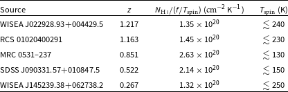
Such spin temperatures are typical of the Milky Way ( $T_\textrm{spin} \lesssim 300$
K, Strasser & Taylor Reference Strasser and Taylor2004; Dickey et al. Reference Dickey, Strasser, Gaensler, Haverkorn, Kavars, McClure-Griffiths, Stil and Taylor2009), but may be atypical in sources host to a powerful AGN. As mentioned in Section 3.1.1, the ionising photon rate is only available for one of these (WISEA J145239.38+062738.2), which has
$T_\textrm{spin} \lesssim 300$
K, Strasser & Taylor Reference Strasser and Taylor2004; Dickey et al. Reference Dickey, Strasser, Gaensler, Haverkorn, Kavars, McClure-Griffiths, Stil and Taylor2009), but may be atypical in sources host to a powerful AGN. As mentioned in Section 3.1.1, the ionising photon rate is only available for one of these (WISEA J145239.38+062738.2), which has $Q_{{\textrm{H}\,\scriptsize{\textrm{I}}}} = 2.4\times10^{53}$
s
$Q_{{\textrm{H}\,\scriptsize{\textrm{I}}}} = 2.4\times10^{53}$
s $^{-1}$
. This is three orders of magnitude below the highest value where H i has been detected. Furthermore, this, and the other three high column density systems, are at redshifts
$^{-1}$
. This is three orders of magnitude below the highest value where H i has been detected. Furthermore, this, and the other three high column density systems, are at redshifts $z\ll 3$
, meaning that the optical-band observation which yielded the redshift are not close to the rest-frame UV band. This was identified as introducing a possible bias by Curran et al. Reference Curran, Whiting, Wiklind, Webb, Murphy and Purcell(2008b
), where the selection of objects faint in the B-band at
$z\ll 3$
, meaning that the optical-band observation which yielded the redshift are not close to the rest-frame UV band. This was identified as introducing a possible bias by Curran et al. Reference Curran, Whiting, Wiklind, Webb, Murphy and Purcell(2008b
), where the selection of objects faint in the B-band at $z \gtrsim 3$
, which were sufficiently bright to yield an optical redshift, selected only objects which were very UV luminous in the source rest-frame.
$z \gtrsim 3$
, which were sufficiently bright to yield an optical redshift, selected only objects which were very UV luminous in the source rest-frame.
Of the three high redshift exceptions where H i has been detected, twoFootnote h have relatively low photo-ionisation rates ( $Q_{{\textrm{H}\,\scriptsize{\textrm{I}}}} \lesssim 10^{54}$
s
$Q_{{\textrm{H}\,\scriptsize{\textrm{I}}}} \lesssim 10^{54}$
s $^{-1}$
, see Fig. 3). For these, the redshifts were obtained from spectroscopy of the near-infrared band (Lawrence, Cohen, & Oke 1995; Lilly, Longair, & Allington-Smith Reference Lilly, Longair and Allington-Smith1985, respectively), thus remaining clear of the rest-frame
$^{-1}$
, see Fig. 3). For these, the redshifts were obtained from spectroscopy of the near-infrared band (Lawrence, Cohen, & Oke 1995; Lilly, Longair, & Allington-Smith Reference Lilly, Longair and Allington-Smith1985, respectively), thus remaining clear of the rest-frame $\lambda\leq1216$
Å range, where the hydrogen becomes excited and subsequently ionised. For the other
$\lambda\leq1216$
Å range, where the hydrogen becomes excited and subsequently ionised. For the other $z\gtrsim 3$
detection (8C 0604+728 at
$z\gtrsim 3$
detection (8C 0604+728 at $z = 3.530$
, Aditya et al. Reference Aditya, Jorgenson, Joshi, Singh, An and Chandola2021), the redshift was obtained by deep optical observations towards a previously identified radio source (Jorgenson et al. Reference Jorgenson, Wolfe, Prochaska, Lu, Howk, Cooke, Gawiser and Gelino2006).Footnote i
$z = 3.530$
, Aditya et al. Reference Aditya, Jorgenson, Joshi, Singh, An and Chandola2021), the redshift was obtained by deep optical observations towards a previously identified radio source (Jorgenson et al. Reference Jorgenson, Wolfe, Prochaska, Lu, Howk, Cooke, Gawiser and Gelino2006).Footnote i
3.3. H i 21-cm absorption at the highest ionisation rate
From our fitting, the highest ionising photon rate at which H i absorption has been detected (Aditya & Kanekar Reference Aditya and Kanekar2018a
) occurs at $Q_{{\textrm{H}\,\scriptsize{\textrm{I}}}} = 2.9\times10^{56}$
s
$Q_{{\textrm{H}\,\scriptsize{\textrm{I}}}} = 2.9\times10^{56}$
s $^{-1}$
, in PKS 1200+045 at
$^{-1}$
, in PKS 1200+045 at $z=1.226$
(Fig. 6). This is the same as the theoretical
$z=1.226$
(Fig. 6). This is the same as the theoretical $Q_{{\textrm{H}\,\scriptsize{\textrm{I}}}}$
required to ionise all of the gas in the Milky Way (Curran & Whiting Reference Curran and Whiting2012). However, this was based on the simple exponential distribution, which we have shown to overestimate the column density (Section 3.2).
$Q_{{\textrm{H}\,\scriptsize{\textrm{I}}}}$
required to ionise all of the gas in the Milky Way (Curran & Whiting Reference Curran and Whiting2012). However, this was based on the simple exponential distribution, which we have shown to overestimate the column density (Section 3.2).
To obtain a revised value of the critical ionising photon rate, we again start with the ionisation and recombination of the gas in equilibrium (Osterbrock Reference Osterbrock1989),
 \begin{equation}Q_{{{\textrm{H}\,\scriptsize{\textrm{I}}}}}= 4\pi\int^{r_\textrm{str}}_{0}\,n_\textrm{p}\,n_\textrm{e}\,\alpha_{A}\,r^2\, dr\end{equation}
where $n_\textrm{p}$
and
$n_\textrm{p}$
and $n_\textrm{e}$
are the proton and electron densities, respectively, and
$n_\textrm{e}$
are the proton and electron densities, respectively, and $\alpha_{A}$
the radiative recombination rate coefficient of hydrogen. We use here the canonical
$\alpha_{A}$
the radiative recombination rate coefficient of hydrogen. We use here the canonical $T=10\,000$
K for ionised gas, giving
$T=10\,000$
K for ionised gas, giving $\alpha_{A}=4.19\times10^{-13}$
cm
$\alpha_{A}=4.19\times10^{-13}$
cm $^3$
s
$^3$
s $^{-1}$
(Osterbrock & Ferland Reference Osterbrock and Ferland2006).Footnote j For a neutral plasma,
$^{-1}$
(Osterbrock & Ferland Reference Osterbrock and Ferland2006).Footnote j For a neutral plasma, $n_\textrm{p}=n_\textrm{e}=n$
, and complete ionisation of the gas (
$n_\textrm{p}=n_\textrm{e}=n$
, and complete ionisation of the gas ( $r_\textrm{str}=\infty$
), the compound model gives
$r_\textrm{str}=\infty$
), the compound model gives
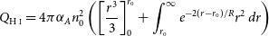 \begin{equation}Q_{{{\textrm{H}\,\scriptsize{\textrm{I}}}}}= 4\pi \alpha_{A} n_0^2 \left(\left[\frac{r^3}{3}\right]_0^{r_0} + \int^{\infty}_{r_0} e^{-2(r-r_0)/R} r^2\, dr\right)\end{equation}
 \begin{equation}\;\;\;\;\;\;= \pi \alpha_{A} n_0^2 \left(\frac{4r_0^3}{3} + R\left[2r_0^2 + 2Rr_0 + R^2\right]\right),\end{equation}
which for $r_0 = 0$
becomes the simple exponential model at large radii,
$r_0 = 0$
becomes the simple exponential model at large radii, $Q_{{{\textrm{H}\,\scriptsize{\textrm{I}}}}}= \pi \alpha_{A} n_0^2R^3$
(Curran & Whiting Reference Curran and Whiting2012). An important feature of this is that the radius of the Strömgren sphere becomes infinite for a finite photo-ionisation rate, giving the abrupt cut-off in H i detections seen in the observations.
$Q_{{{\textrm{H}\,\scriptsize{\textrm{I}}}}}= \pi \alpha_{A} n_0^2R^3$
(Curran & Whiting Reference Curran and Whiting2012). An important feature of this is that the radius of the Strömgren sphere becomes infinite for a finite photo-ionisation rate, giving the abrupt cut-off in H i detections seen in the observations.
From Equation (12), the ionising photon rate to ionise all of the gas in the Milky Way is revised to $Q_{{\textrm{H}\,\scriptsize{\textrm{I}}}} =7.6\times10^{55}$
s
$Q_{{\textrm{H}\,\scriptsize{\textrm{I}}}} =7.6\times10^{55}$
s $^{-1}$
, which is a factor of four lower than for the simple exponential model. Of course all of gas need not be ionised to be rendered below the detection limits of current radio telescopes, although the apparently abrupt cut-off in the detection of H i at
$^{-1}$
, which is a factor of four lower than for the simple exponential model. Of course all of gas need not be ionised to be rendered below the detection limits of current radio telescopes, although the apparently abrupt cut-off in the detection of H i at $Q_{{\textrm{H}\,\scriptsize{\textrm{I}}}} \lesssim 10^{56}$
s
$Q_{{\textrm{H}\,\scriptsize{\textrm{I}}}} \lesssim 10^{56}$
s $^{-1}$
has persisted in all of the published searches since Curran et al. Reference Curran, Whiting, Wiklind, Webb, Murphy and Purcell(2008b
) [see Section 1].
$^{-1}$
has persisted in all of the published searches since Curran et al. Reference Curran, Whiting, Wiklind, Webb, Murphy and Purcell(2008b
) [see Section 1].
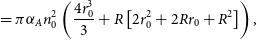
In Fig. 9 we show the ‘tweaking’ required to the Galactic gas distribution to increase the critical value to $Q_{{\textrm{H}\,\scriptsize{\textrm{I}}}} = 2.9\times10^{56}$
s
$Q_{{\textrm{H}\,\scriptsize{\textrm{I}}}} = 2.9\times10^{56}$
s $^{-1}$
. For example, for the same values of R and
$^{-1}$
. For example, for the same values of R and $r_0$
as the Milky Way, the central density would have to be doubled to
$r_0$
as the Milky Way, the central density would have to be doubled to $n_0=2.9$ $\textrm{cm}^{-3}$
. Conversely, keeping
$\textrm{cm}^{-3}$
. Conversely, keeping $n_0=1.45$ $\textrm{cm}^{-3}$
gives the values of
$\textrm{cm}^{-3}$
gives the values of $r_0$
and R listed in Table 2.
$r_0$
and R listed in Table 2.
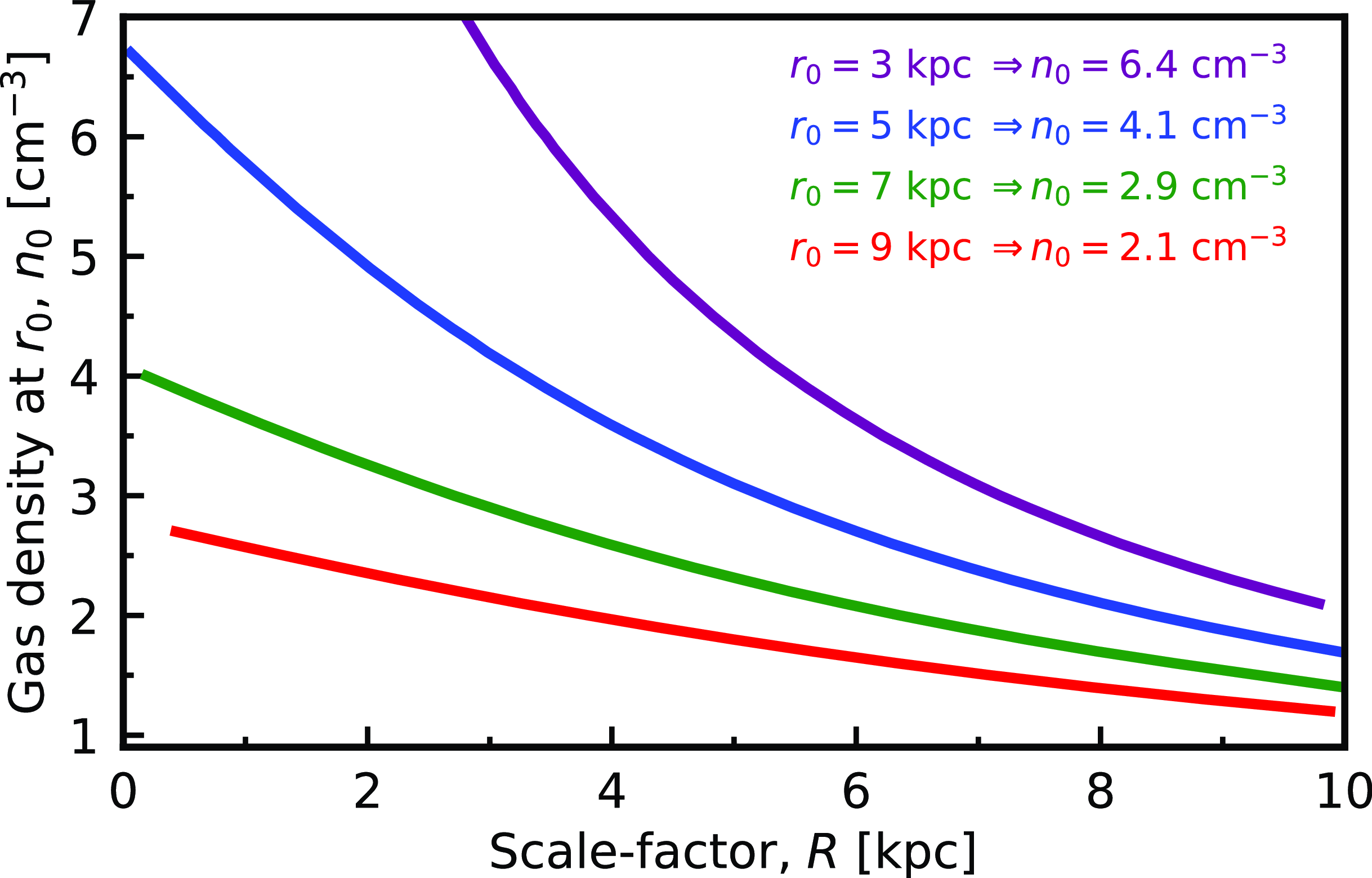
Figure 9. The gas density at $r_0$
versus the scale-length required for all of the gas to be ionised by
$r_0$
versus the scale-length required for all of the gas to be ionised by $Q_{{\textrm{H}\,\scriptsize{\textrm{I}}}} = 2.9\times10^{56}$
s
$Q_{{\textrm{H}\,\scriptsize{\textrm{I}}}} = 2.9\times10^{56}$
s $^{-1}$
.
$^{-1}$
. $r_0 = 7$
kpc for the Milky Way (Kalberla & Kerp Reference Kalberla and Kerp2009) and the key shows the value of
$r_0 = 7$
kpc for the Milky Way (Kalberla & Kerp Reference Kalberla and Kerp2009) and the key shows the value of $n_0$
required for the Milky Way’s
$n_0$
required for the Milky Way’s $R=3.15$
kpc.
$R=3.15$
kpc.
From these parameters we estimate column densities which are approximately equal to the maximum expected (Section 3.2) and use these to estimate possible $T_\textrm{spin}/f$
values, all of which are very high. While low covering factors (
$T_\textrm{spin}/f$
values, all of which are very high. While low covering factors ( $f\ll1$
) could contribute to these, high spin temperatures would be expected from the strong UV continuum (Field Reference Field1959; Bahcall & Ekers Reference Bahcall and Ekers1969).Footnote k
$f\ll1$
) could contribute to these, high spin temperatures would be expected from the strong UV continuum (Field Reference Field1959; Bahcall & Ekers Reference Bahcall and Ekers1969).Footnote k
In the table we also show the total gas masses, obtained from $M_\textrm{ gas} = \int_0^{\infty}\rho dV$
, where the volume of the disc gives
$M_\textrm{ gas} = \int_0^{\infty}\rho dV$
, where the volume of the disc gives $dV = 2\pi tr dr$
, with t being its thickness. In the Galaxy the thickness is related to the galactocentric radius via the flare factor,
$dV = 2\pi tr dr$
, with t being its thickness. In the Galaxy the thickness is related to the galactocentric radius via the flare factor, $F = r/t\approx20$
(Kalberla & Kerp Reference Kalberla and Kerp2009), giving for the compound model:
$F = r/t\approx20$
(Kalberla & Kerp Reference Kalberla and Kerp2009), giving for the compound model:
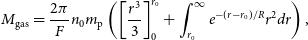 \begin{equation} M_\textrm{gas} = \frac{2\pi}{F} n_0 m_\textrm{p}\left(\left[\frac{r^3}{3}\right]_0^{r_0} + \int_{r_0}^{\infty}e^{-(r-r_0)/R}r^2dr\right),\end{equation}
which gives
 \begin{equation}M_\textrm{gas} = \frac{2\pi}{F} n_0 m_\textrm{p}\left(\frac{r_0^3}{3} + R\left[r_0^2 + 2Rr_0 + 2R^2\right]\right).\end{equation}
The H i masses derived from Equation (14) (Table 2) are close to the maximum observed in 1 000 low redshift galaxies ( $M_\textrm{gas} = 4\times10^{10}$
M
$M_\textrm{gas} = 4\times10^{10}$
M $_\odot$
, Koribalski et al. Reference Koribalski2004), indicating that
$_\odot$
, Koribalski et al. Reference Koribalski2004), indicating that $Q_{{\textrm{H}\,\scriptsize{\textrm{I}}}}\sim3\times10^{56}$
s
$Q_{{\textrm{H}\,\scriptsize{\textrm{I}}}}\sim3\times10^{56}$
s $^{-1}$
is approaching the critical value above which all of the gas in most galaxies will be ionised.
$^{-1}$
is approaching the critical value above which all of the gas in most galaxies will be ionised.
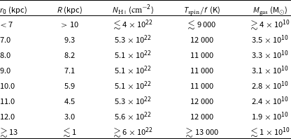
Table 2. The required scale-length for various values of $r_0$
to yield complete ionisation for
$r_0$
to yield complete ionisation for $Q_{{\textrm{H}\,\scriptsize{\textrm{I}}}} = 2.9\times10^{56}$
s
$Q_{{\textrm{H}\,\scriptsize{\textrm{I}}}} = 2.9\times10^{56}$
s $^{-1}$
and
$^{-1}$
and $n_0=1.45$ $\textrm{cm}^{-3}$
. The column densities are calculated from Equation (9) and
$\textrm{cm}^{-3}$
. The column densities are calculated from Equation (9) and $T_\textrm{spin}/f$
from the measured
$T_\textrm{spin}/f$
from the measured $N_{{{\textrm{H}\,\scriptsize{\textrm{I}}}}} = 4.6\times10^{18}\,(T_\textrm{spin}/f)$ $\textrm{cm}^{-2}$
(Aditya & Kanekar Reference Aditya and Kanekar2018a
). The gas masses are calculated from Equation (14) using the Galactic flare factor (Kalberla & Kerp Reference Kalberla and Kerp2009).
$\textrm{cm}^{-2}$
(Aditya & Kanekar Reference Aditya and Kanekar2018a
). The gas masses are calculated from Equation (14) using the Galactic flare factor (Kalberla & Kerp Reference Kalberla and Kerp2009).
4. Conclusions
From the complete photometry of each of the 924 $z\geq0.1$
radio sources searched for in H i 21-cm absorption, we have collated the ionising photon rates and radio luminosities, finding:
$z\geq0.1$
radio sources searched for in H i 21-cm absorption, we have collated the ionising photon rates and radio luminosities, finding:
-
• The highest ionising photon rate at which H i has been detected remains
$Q_{{\textrm{H}\,\scriptsize{\textrm{I}}}} \approx 3\times10^{56}$
s
$^{-1}$
, which is close to the value required to ionise all of the neutral gas in a large spiral galaxy, thus confirming that the dearth of H i detections at high redshift is due to the bias towards sources which are most UV luminous in the rest-frame. -
• Both the ionising photon rate and radio luminosity are anti-correlated with the strength of the H i absorption, although the
$Q_{{{\textrm{H}\,\scriptsize{\textrm{I}}}}}$
correlation is the strongest. Also, unlike the ionising photon rate, there is no critical radio luminosity above which H i is not detected. That is, ionisation of the gas, rather than excitation to the upper hyper-fine level, appears to be the dominant mechanism for the dearth of H i absorption at high redshift. -
• Any evolution in the source morphologies or gas properties cannot explain the decrease in detection rate with redshift as holistically as the ionisation hypothesis.
-
• Detections rates are higher in galaxies than in quasars, which we attribute to the quasars generally being more luminous in the UV. It is possible that orientation effects play a role, although being a type 1 object does not necessarily exclude the detection of H i absorption. This suggests that the absorption primarily occurs in the large-scale galactic disc, as opposed to the pc-scale obscuring torus.


From the total neutral hydrogen column density of the Milky Way (Kalberla & Kerp Reference Kalberla and Kerp2009), and that expected from theory, we find:
-
• The strengths of the five recently detected H i absorbers with
$N_{{{\textrm{H}\,\scriptsize{\textrm{I}}}}} \gtrsim 10^{20}\,(T_\textrm{spin}/f)$
$\textrm{cm}^{-2}$
(Chowdhury et al. Reference Chowdhury, Kanekar and Chengalur2020; Murthy et al. Reference Murthy, Morganti, Oosterloo and Maccagni2021; Su et al. Reference Su2022; Aditya et al. Reference Aditya2024), imply spin temperatures of
$T_\textrm{spin}/f \lesssim 300$
K, which are typical of the Milky Way (Strasser & Taylor Reference Strasser and Taylor2004; Dickey et al. Reference Dickey, Strasser, Gaensler, Haverkorn, Kavars, McClure-Griffiths, Stil and Taylor2009). Sufficient UV photometry to obtain the ionising photon rate is only available for one of these, but with
$Q_{{\textrm{H}\,\scriptsize{\textrm{I}}}} = 2.4\times10^{53}$
s
$^{-1}$
this is three orders of magnitude below the critical value above which we expect all of the gas to be ionised. -
• Conversely, for the detection of H i at the highest ionising photon rate (
$Q_{{\textrm{H}\,\scriptsize{\textrm{I}}}} =2.9\times10^{56}$
s
$^{-1}$
), we estimate
$T_\textrm{spin}/f\sim12\,000$
K which is consistent with a high ionisation fraction. -
• At this ionising photon rate we calculate a gas mass of
$M_\textrm{gas} \approx3\times10^{10}$
M
$_\odot$
, which is close to the maximum value observed in a survey of a 1 000 low redshift galaxies (Koribalski et al. Reference Koribalski2004).


The model is, of course, an idealisation, based upon the gas distribution of the Milky Way and taking no account of shielding by dustFootnote l or regions of denser gas (e.g. molecular clouds). However, it is remarkable that it comes close to yielding the maximum ionising photon rate at which H i has been detected for a gas distribution so similar to that of a large spiral galaxy. Thus, both the extensive observational results and the model suggest that ionisation by $\lambda\leq912$
Å photons is the dominant reason for the non-detection of cold, neutral gas within the host galaxies of high redshift radio sources.
$\lambda\leq912$
Å photons is the dominant reason for the non-detection of cold, neutral gas within the host galaxies of high redshift radio sources.
Acknowledgements
I would like the thank the anonymous referee for their prompt and supportive feedback. This research has made use of the NASA/IPAC Extragalactic Database (NED) which is operated by the Jet Propulsion Laboratory, California Institute of Technology, under contract with the National Aeronautics and Space Administration and NASA’s Astrophysics Data System Bibliographic Service. This research has also made use of NASA’s Astrophysics Data System Bibliographic Service and asurv Rev 1.2 (Lavalley, Isobe, & Feigelson Reference Lavalley, Isobe and Feigelson1992), which implements the methods presented in Isobe et al. (Reference Isobe, Feigelson and Nelson1986).
Data availability
Data available on request.


 Open access