


1. Introduction
One of the primary focuses in radio astronomy science is understanding the early Universe formation history. Although the redshift boundary where ionised gas recombined into neutral hydrogen is well measureable through the cosmic microwave background (CMB) (Komatsu et al. Reference Komatsu2009), the redshift region of the birth of the first stars, during the cosmic dawn (CD), and the absolute redshift boundaries of the epoch of reionisation (EoR) remain uncertain. Observing and better constraining the redshift regions of these epochs is therefore key to gain a better understanding of the formation history of our Universe; as well as early stages of cosmic structure formation, where presently almost nothing is known. (Furlanetto, Oh, & Briggs Reference Furlanetto, Oh and Briggs2006).
Much effort has been put in to attempt to constrain the boundaries of the EoR through directly probing the intergalactic medium (IGM), for example, determining the anisotropies in the CMB due to Thompson Scattering and calculating the optical depth limit (Holder et al. Reference Holder, Haiman, Kaplinghat and Knox2003; Planck Collaboration XIII Reference Planck Collaboration2016), measuring the scattering effects caused by Lyman-Alpha emitters (Dijkstra Reference Dijkstra2016), measuring Gunn-Peterson absorption at high-redshift quasar spectra caused by quasar damping wings (Fan, Carilli, & Keating Reference Fan, Carilli and Keating2006), and probing the 21 cm spectral line of neutral hydrogen (Furlanetto, Sokasian, & Hernquist Reference Furlanetto, Sokasian and Hernquist2004). Results from recent studies lead us to believe the bounds of the EoR are somewhere between a redshift of $z\sim\{5.4\!-\!10\}$
(Kulkarni et al. Reference Kulkarni, Keating, Haehnelt, Bosman, Puchwein, Chardin and Aubert2019; Nasir & D’Aloisio Reference Nasir and D’Aloisio2020; Planck Collaboration XIII Reference Planck Collaboration2016).
$z\sim\{5.4\!-\!10\}$
(Kulkarni et al. Reference Kulkarni, Keating, Haehnelt, Bosman, Puchwein, Chardin and Aubert2019; Nasir & D’Aloisio Reference Nasir and D’Aloisio2020; Planck Collaboration XIII Reference Planck Collaboration2016).
However, detecting the 21 cm line does not come without challenges. One of the biggest challenges to detect this signal is that it is hidden within the foregrounds. Foregrounds consist of relatively compact emission from extra-galactic sources (active galactic nuclei AGN and star-forming galaxies) and diffuse polarised emission due to galactic synchrotron radiation, which have angular scales from 10’s of arcminutes to the entire sky. These foregrounds are generally three to five orders of magnitude brighter than the signal we desire to detect (Morales & Wyithe Reference Morales and Wyithe2010; Vedantham, Udaya Shankar, & Subrahmanyan Reference Vedantham, Udaya Shankar and Subrahmanyan2012; Mertens, Ghosh, & Koopmans Reference Mertens, Ghosh and Koopmans2018; Trott et al. Reference Trott2020; Ghosh et al. 2020). In order to solve for this, foreground mitigation methods have to be employed. Ideally, one would characterise these foregrounds on a wide range of angular scales and frequencies, through the generation of high resolution all-sky maps (Eastwood et al. Reference Eastwood2018) and create a model for foreground subtraction.
Generating a comprehensive EoR foreground model requires a combination of both compact components and a diffuse component. Compact source information can be obtained from one of the many interferometric surveys that cover large areas of the sky, for example, GLEAM (Wayth et al. Reference Wayth2015), TGSS (Intema et al. Reference Intema, Jagannathan, Mooley and Frail2017), and LoTSS (Williams et al. Reference Williams2019), and the source catalogues that result from them. However, compact source catalogues do not describe diffuse emission and the galactic plane is often excluded due to the complexity of imaging those regions with interferometers.
Mapping the diffuse emission, simultaneously in the galactic plane and outside it, is a challenging process. The well-known Haslam sky map (Haslam et al. Reference Haslam1981, Reference Haslam, Salter, Stoffel and Wilson1982) has been the most prominent in use over the past few decades as a low frequency sky model. However, the need for more diffuse sky maps over a wider frequency range sparked the increase in these maps through a multitude of sky surveys. The most prominent diffuse sky maps generated since the Haslam map are the GSM (De Oliveira-Costa et al. Reference De Oliveira-Costa2008), S-PASS 2.3 GHz Polarisation Survey (Carretti et al. Reference Carretti2019), CHIPASS (Calabretta, Staveley-Smith, & Barnes Reference Calabretta, Staveley-Smith and Barnes2014), LWA-LFSS (Dowell et al. Reference Dowell2017), recalibrated versions of the 150 MHz diffuse sky map by Landecker & Wielebinski (Reference Landecker and Wielebinski1970) (Patra et al. Reference Patra, Subrahmanyan, Sethi, Udaya Shankar and Raghunathan2015; Monsalve et al. Reference Monsalve2021), and the 45 MHz diffuse map by Guzmán et al. (Reference Guzmán, May, Alvarez and Maeda2010). Although a significant improvement, more maps have to be generated at more areas on the sky and at more frequencies to provide an accurate diffuse foreground model; especially the lower frequency regime and the southern hemisphere.
Eastwood et al. (Reference Eastwood2018) started to address these issues by generating low-frequency high resolution (around ${\sim}15$
arcmin) northern sky maps using the Owens Valley Radio Observatory Long Wavelength Array (OVRO-LWA) (Kassim et al. Reference Kassim2005) interferometer array using a whole different imaging method altogether. Eastwood et al. (Reference Eastwood2018) employed a method known as the Tikhonov-regularised m-mode formalism; an adaption to the spherical harmonic transit interferometric imaging method suggested by Shaw et al. (Reference Shaw, Sigurdson, Pen, Stebbins and Sitwell2014, Reference Shaw, Sigurdson, Sitwell, Stebbins and Pen2015). Opposite to traditional radio interferometry, the m-mode formalism no longer utilises snapshot visibilities to image the sky, but uses components of timescale variations within these visibilities instead. The formalism uses these components to rebuild the sky using spherical harmonic basis functions. Since these basis functions operate over the full celestial sphere, tracking the time variance components across a full sidereal day allows one to reconstruct the full sky in a single imaging step whilst maintaining exact widefield accuracy.
${\sim}15$
arcmin) northern sky maps using the Owens Valley Radio Observatory Long Wavelength Array (OVRO-LWA) (Kassim et al. Reference Kassim2005) interferometer array using a whole different imaging method altogether. Eastwood et al. (Reference Eastwood2018) employed a method known as the Tikhonov-regularised m-mode formalism; an adaption to the spherical harmonic transit interferometric imaging method suggested by Shaw et al. (Reference Shaw, Sigurdson, Pen, Stebbins and Sitwell2014, Reference Shaw, Sigurdson, Sitwell, Stebbins and Pen2015). Opposite to traditional radio interferometry, the m-mode formalism no longer utilises snapshot visibilities to image the sky, but uses components of timescale variations within these visibilities instead. The formalism uses these components to rebuild the sky using spherical harmonic basis functions. Since these basis functions operate over the full celestial sphere, tracking the time variance components across a full sidereal day allows one to reconstruct the full sky in a single imaging step whilst maintaining exact widefield accuracy.
In this paper, we aim to complement the existing diffuse low-frequency sky maps by generating a low-frequency southern sky map at 159 MHz using the Engineering Development Array 2 (EDA2) (Wayth et al. Reference Wayth2021), which is a prototype station of the future SKA-Low (Braun et al. Reference Braun, Bourke, Green, Keane and Wagg2015). For the generation of this sky map we also employ the m-mode formalism. This allows us to take full advantage of the EDA2’s wide field of view (FoV), allowing us to hyper-resolve the spatial scales on the sky with full widefield accuracy. We also introduce the concept of spherical-harmonic beam coverage, an analogy to measure for completeness on the sky similar to the $u, v$
-coverage in traditional interferometry. Additionally, an image-based spherical harmonic CLEANing algorithm is presented, significantly reducing the number of unique point-sources that need to be generated, whilst maintaining the ability to accurately deconvolve point-spread functions (PSFs).
$u, v$
-coverage in traditional interferometry. Additionally, an image-based spherical harmonic CLEANing algorithm is presented, significantly reducing the number of unique point-sources that need to be generated, whilst maintaining the ability to accurately deconvolve point-spread functions (PSFs).
2. All-sky interferometry
In radio astronomy—and interferometry imaging algorithms in general—the goal is to determine the sky brightness temperature $\textrm{T}_{\textrm{b},\nu}(\hat{\textbf{n}})$
or sky intensity
$\textrm{T}_{\textrm{b},\nu}(\hat{\textbf{n}})$
or sky intensity $\textrm{I}_{\nu}(\hat{\textbf{n}})$
for a specific pointing
$\textrm{I}_{\nu}(\hat{\textbf{n}})$
for a specific pointing $\hat{\textbf{n}}$
on the celestial sphere, with quasi-monochromatic frequency
$\hat{\textbf{n}}$
on the celestial sphere, with quasi-monochromatic frequency $\nu$
. However, an interferometer cannot measure this directly; instead it sees the correlated voltage response between two antenna elements
$\nu$
. However, an interferometer cannot measure this directly; instead it sees the correlated voltage response between two antenna elements ${\big\langle{\textsf{U}}_{\nu}^\textrm{i}(t){\textsf{U}}_{\nu}^\textrm{j*}(t)\big\rangle}$
. Ignoring the polarisation responses, we can define the relation between the measured response and the brightness temperature of the sky as (Thompson, Moran, & Swenson George Reference Thompson, Moran and Swenson George2017; Shaw et al. Reference Shaw, Sigurdson, Pen, Stebbins and Sitwell2014)
${\big\langle{\textsf{U}}_{\nu}^\textrm{i}(t){\textsf{U}}_{\nu}^\textrm{j*}(t)\big\rangle}$
. Ignoring the polarisation responses, we can define the relation between the measured response and the brightness temperature of the sky as (Thompson, Moran, & Swenson George Reference Thompson, Moran and Swenson George2017; Shaw et al. Reference Shaw, Sigurdson, Pen, Stebbins and Sitwell2014)
 \begin{align} V_{\nu}^{\rm ij} = \int B_{\nu}^{\rm ij}(\hat{\textbf{n}}){\rm T}_{\nu}(\hat{\textbf{n}})d^2\hat{\textbf{n}}\,,\,\text{and} \end{align}
 \begin{align} B_{\nu}^{\rm ij}(\hat{\textbf{n}}) = \frac{1}{\sqrt{\Omega_{\rm i}\Omega_{\rm j}}}A_{\nu}^{\rm i}(\hat{\textbf{n}})A_{\nu}^{\rm j*}(\hat{\textbf{n}})e^{2\pi i\hat{\textbf{n}}\cdot{\textbf{u}}_{{ij}}}.\end{align}
In Equation (1) $B_{\nu}^\textrm{ij}$
is the transfer function that encapsulates the system response on the sky,
$B_{\nu}^\textrm{ij}$
is the transfer function that encapsulates the system response on the sky, $A_{\nu}^\textrm{i}$
is the primary beam voltage response of antenna element
$A_{\nu}^\textrm{i}$
is the primary beam voltage response of antenna element $\rm i$
,
$\rm i$
, ${\textbf{u}}_{\textrm{ij}}$
is the separation between two antenna elements—in the
${\textbf{u}}_{\textrm{ij}}$
is the separation between two antenna elements—in the $u, v$
-plane—normalised by the wavelength
$u, v$
-plane—normalised by the wavelength $\lambda$
, and
$\lambda$
, and $\Omega_{\textrm{i}}$
is the beam solid angle of antenna element
$\Omega_{\textrm{i}}$
is the beam solid angle of antenna element $\rm i$
.
$\rm i$
.
Although Equation (1) is a perfectly valid description of the measured voltage response over the full celestial sphere, Eastwood et al. (Reference Eastwood2018) has shown that directly solving for the three-dimensional equation, due to computational cost and complexity, is not a tangible solution. Alternatively, one could assume a flat sky reducing the measurement equation to a two-dimensional Fourier transform. However, this concept starts breaking down for wide FoVs as the curvature of the sky starts playing a role, which the 2D transform does not account for (Carozzi Reference Carozzi2015; Presley, Liu, & Parsons Reference Presley, Liu and Parsons2015; Singh et al. Reference Singh, Subrahmanyan, Udaya Shankar and Raghunathan2015; Thyagarajan et al. Reference Thyagarajan2015a, Reference Thyagarajan2015b; Thompson et al. Reference Thompson, Moran and Swenson George2017). Additionally, the flat-sky approach restricts the capability to image the full-sky in a single imaging sweep, as one cannot distinguish between points on different hemispheres. As a result, one has to resort to making individual snapshots of the sky and, for example, mosaic them together; restricting one to information only available in each individual snapshot.
2.1. Spherical harmonic transit interferometry
To address the issues and complexities of all-sky interferometry, Shaw et al. (Reference Shaw, Sigurdson, Pen, Stebbins and Sitwell2014) proposed spherical harmonic transit interferometry as an alternate solution. Instead of phase-tracking sources with a narrow FoV and mosaicing/stacking the resulting images together to create an image of the full sky, the issues of solving Equation (1) are avoided altogether.
With transit interferometry, the element’s wide FoVs is pointed at zenith to observe the sky in transit over a sidereal day. This allows one to then utilise spherical harmonics to describe the interaction of radio waves emitted by celestial bodies on the observed celestial sphere.
2.2. Spherical harmonics
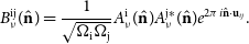
Much similar to how the Fourier series describes how periodic functions interact on a circle, spherical harmonics describe the rate of change (angular frequency) of functions on a sphere. Especially the Laplacian spherical harmonics—derived by expanding the Laplacian in three dimensions—are of interest, as they form an orthonormal basis. In other words, any function that acts on a spherical surface can be expanded into a sum of these Laplacian spherical harmonics; akin to how varying functions restricted to a circle can be expanded into a series of circular functions—that is sines and cosines—using a Fourier transform. An example of the Laplacian spherical harmonics can be seen in Figure 1.
Figure 1. Types of spherical harmonics. Left: sectoral spherical harmonic (a function of $e^{im\varphi}$
) with
$e^{im\varphi}$
) with $m=4$
, Middle: tesseral spherical harmonic (a function of
$m=4$
, Middle: tesseral spherical harmonic (a function of $P_{l}^{|m|}\left(\cos\theta\right)e^{im\varphi}$
) with
$P_{l}^{|m|}\left(\cos\theta\right)e^{im\varphi}$
) with $l=4$
and
$l=4$
and $m=2$
, Right: zonal spherical harmonic (a function of
$m=2$
, Right: zonal spherical harmonic (a function of $P_{l}^{|m|}\left(\cos\theta\right)$
) with
$P_{l}^{|m|}\left(\cos\theta\right)$
) with $l=4$
and
$l=4$
and $m=0$
. Angular velocity of the basis functions, with respect to right ascension (RA), are a function of
$m=0$
. Angular velocity of the basis functions, with respect to right ascension (RA), are a function of $e^{im\phi}$
.
$e^{im\phi}$
.
Spherical Harmonics can be divided into three different categories with regards to how wave forms interact on the sphere. The zonal spherical harmonics (Figure 1, right image) only have variation in the latitudinal direction ( $\theta$
), the sectoral spherical harmonics (Figure 1, left image) only have variation in the longitudinal direction (
$\theta$
), the sectoral spherical harmonics (Figure 1, left image) only have variation in the longitudinal direction ( $\varphi$
), and the tesseral spherical harmonics (Figure 1, middle image) have variation in both the latitudinal and longitudinal direction. This is convenient, as this allows us to express any continuous waveform into subsets of basis functions that describes the waveform’s angular dependencies on both coordinates axes
$\varphi$
), and the tesseral spherical harmonics (Figure 1, middle image) have variation in both the latitudinal and longitudinal direction. This is convenient, as this allows us to express any continuous waveform into subsets of basis functions that describes the waveform’s angular dependencies on both coordinates axes $(\varphi,\theta)$
 \begin{align} Y_{l}^{m}\left(\varphi,\theta\right) &= \sqrt{\frac{2l+1}{4\pi}\frac{\left(l-|m|\right)!}{\left(l+|m|\right)!}}P_{l}^{|m|}\left(\cos\theta\right)e^{im\varphi}.\end{align}
Here, $Y_{l}^{m}\left(\varphi,\theta\right)$
are the complex Laplace spherical harmonics,
$Y_{l}^{m}\left(\varphi,\theta\right)$
are the complex Laplace spherical harmonics, $P_{l}^{|m|}\left(\cos\theta\right)$
are the associated Legendre polynomials,Footnote a and
$P_{l}^{|m|}\left(\cos\theta\right)$
are the associated Legendre polynomials,Footnote a and $e^{im\varphi}$
is Euler’s formula with dependence on m. The components l and m describe the degree and rank of the function respectively, where
$e^{im\varphi}$
is Euler’s formula with dependence on m. The components l and m describe the degree and rank of the function respectively, where $l\,\in\,\mathbb{Z}^{0+}$
and
$l\,\in\,\mathbb{Z}^{0+}$
and $-l\,\leq\,m\,\leq\,l$
. Simply said, the degree l describes the number of cross-sections on the sphere, of which
$-l\,\leq\,m\,\leq\,l$
. Simply said, the degree l describes the number of cross-sections on the sphere, of which $|m|$
are longitudinal functions and
$|m|$
are longitudinal functions and $l-|m|$
are latitudinal functions.
$l-|m|$
are latitudinal functions.
2.3. The m-mode formalism
In order to leverage spherical harmonics to describe functions across the sky, we align the spherical coordinate system with the celestial sphere. Doing so, $\varphi$
describes the celestial plane’s right ascension (RA) and
$\varphi$
describes the celestial plane’s right ascension (RA) and $\theta$
describes the declination (DEC). Given that the Earth’s rotation is periodic over a sidereal day (LST) and is explicitly dependent on the azimuthal axis (
$\theta$
describes the declination (DEC). Given that the Earth’s rotation is periodic over a sidereal day (LST) and is explicitly dependent on the azimuthal axis ( $\phi$
), Shaw et al. (Reference Shaw, Sigurdson, Pen, Stebbins and Sitwell2014) concluded that one can take advantage of this Earth rotational symmetry in plane with the sectoral spherical harmonics; using wide FoV interferometers through transit interferometry.
$\phi$
), Shaw et al. (Reference Shaw, Sigurdson, Pen, Stebbins and Sitwell2014) concluded that one can take advantage of this Earth rotational symmetry in plane with the sectoral spherical harmonics; using wide FoV interferometers through transit interferometry.
The topic of spherical harmonic transit interferometry has been extensively covered by Shaw et al. (Reference Shaw, Sigurdson, Pen, Stebbins and Sitwell2014); Shaw et al. (Reference Shaw, Sigurdson, Sitwell, Stebbins and Pen2015) and Eastwood et al. (Reference Eastwood2018). As such, we will only briefly review the key points concerning the m-mode formalism and solving for the sky. However, we highly recommend the interested reader to refer to the aforementioned papers for a more complete overview.
Using zenith pointed observations and measure over a full sidereal day would therefore make the three-dimensional measurement equation a function of $\phi$
(Shaw et al. Reference Shaw, Sigurdson, Pen, Stebbins and Sitwell2014):
$\phi$
(Shaw et al. Reference Shaw, Sigurdson, Pen, Stebbins and Sitwell2014):
 \begin{align} V_{\nu}^\textrm{ij}(\phi) &= \int B_{\nu}^\textrm{ij}\left(\hat{\textbf{n}};\ \phi\right)\textrm{T}_{\nu}(\hat{\textbf{n}})d^2\hat{\textbf{n}}\,.\end{align}
Expanding the beam-transfer function (beam $\times$
fringe) into its spherical harmonic coefficients provides a description of the angular and spatial coverage of the interferometer system for a specific baseline and frequency. The beam-transfer function can be expressed as
$\times$
fringe) into its spherical harmonic coefficients provides a description of the angular and spatial coverage of the interferometer system for a specific baseline and frequency. The beam-transfer function can be expressed as
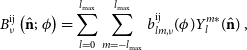 \begin{align} B_{\nu}^\textrm{ij}\left(\hat{\textbf{n}};\ \phi\right) &= \sum\limits_{l=0}^{l_{\textrm{max}}}\sum\limits_{m=-l_{\textrm{max}}}^{l_{\textrm{max}}} b_{lm, \nu}^\textrm{ij}(\phi)Y_{l}^{m*}(\hat{\textbf{n}})\,,\end{align}
where $b_{lm, \nu}^\textrm{ij}(\phi)$
are the spherical harmonic coefficients of the decomposed beam-transfer function. Similarly, we can decompose the sky brightness temperature into a set of spherical harmonic coefficients describing the full spatial coverage across the celestial sphere
$b_{lm, \nu}^\textrm{ij}(\phi)$
are the spherical harmonic coefficients of the decomposed beam-transfer function. Similarly, we can decompose the sky brightness temperature into a set of spherical harmonic coefficients describing the full spatial coverage across the celestial sphere
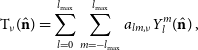 \begin{align} \textrm{T}_{\nu}(\hat{\textbf{n}}) &= \sum\limits_{l=0}^{l_{\textrm{max}}}\sum\limits_{m=-l_{\textrm{max}}}^{l_{\textrm{max}}} a_{lm, \nu}Y_{l}^{m}(\hat{\textbf{n}})\,,\end{align}
where $a_{lm, \nu}$
are the spherical harmonic coefficients of the decomposed sky. It should be noted that in the m-mode definitions by Shaw et al. (Reference Shaw, Sigurdson, Pen, Stebbins and Sitwell2014) the spherical harmonic basis functions in the beam transfer function and sky decomposition are conjugates of each other to ‘simplify later notation’. As a result, due to the fact that spherical harmonics are orthonormal functions, the basis functions drop out of the m-mode equation given that
$a_{lm, \nu}$
are the spherical harmonic coefficients of the decomposed sky. It should be noted that in the m-mode definitions by Shaw et al. (Reference Shaw, Sigurdson, Pen, Stebbins and Sitwell2014) the spherical harmonic basis functions in the beam transfer function and sky decomposition are conjugates of each other to ‘simplify later notation’. As a result, due to the fact that spherical harmonics are orthonormal functions, the basis functions drop out of the m-mode equation given that
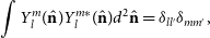 \begin{align} \int Y_{l}^{m}(\hat{\textbf{n}})Y_{l}^{m*}(\hat{\textbf{n}})d^2\hat{\textbf{n}} &= \delta_{ll'}\delta_{mm'},\end{align}
with $\delta_{ll'}$
and
$\delta_{ll'}$
and $\delta_{mm'}$
being Kronecker delta functions.
$\delta_{mm'}$
being Kronecker delta functions.
Closely observing Equation (3), it is clear that m only affects the $\varphi$
coordinate via the phase term
$\varphi$
coordinate via the phase term $e^{im\varphi}$
, which is a rotation in the plane of RA. Any RA displacement in spherical harmonic space is therefore only a function of
$e^{im\varphi}$
, which is a rotation in the plane of RA. Any RA displacement in spherical harmonic space is therefore only a function of $e^{im\varphi}$
. As a result, the rotation (
$e^{im\varphi}$
. As a result, the rotation ( $\phi$
) of the sky for a transit telescope only affects components of the spherical harmonics that change with m. Shaw et al. (Reference Shaw, Sigurdson, Pen, Stebbins and Sitwell2014) concluded that we can thus track components that vary across different timescales over a sidereal day on a per-m-basis. In order to relate what we measure on the sky to the spherical harmonics we can Fourier transform our visibilities with respect to m, such that
$\phi$
) of the sky for a transit telescope only affects components of the spherical harmonics that change with m. Shaw et al. (Reference Shaw, Sigurdson, Pen, Stebbins and Sitwell2014) concluded that we can thus track components that vary across different timescales over a sidereal day on a per-m-basis. In order to relate what we measure on the sky to the spherical harmonics we can Fourier transform our visibilities with respect to m, such that
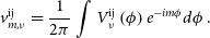 \begin{align} v_{m,\nu}^{\textrm{ij}} &= \frac{1}{2\pi}\int V_{\nu}^\textrm{ij}\left(\phi\right)e^{-im\phi}d\phi\,.\end{align}
This provides us with a formalism where we no longer use information of individual snapshots across the sky, but rather the Fourier components that describe the varying timescales of what of we observe across the sky over a full sidereal day. These components are also known as m-modes. The complete spherical harmonic relation can therefore be defined as
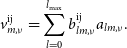 \begin{align} v_{m,\nu}^{\textrm{ij}} &= \sum\limits_{l=0}^{l_{\textrm{max}}} b_{lm,\nu}^\textrm{ij}a_{lm,\nu}.\end{align}
which describes the encoded observed spatial frequency of the whole sky observed through the physical system on an m-by-m basis, also known as the m-mode formalism. The sky coefficients $a_{lm,\nu}$
are then used to reconstruct the sky, acting as weightings for the spherical harmonic basis functions. This allows for us to image the full sky in a single imaging step, maintaining exact widefield accuracy without the introduction of regridding artefacts, since we no longer use individual snapshots. Equation (9) also reduces the measurement equation into a simple linear relation, describing how the sky maps to data obtained through the physical system (Shaw et al. Reference Shaw, Sigurdson, Pen, Stebbins and Sitwell2014)
$a_{lm,\nu}$
are then used to reconstruct the sky, acting as weightings for the spherical harmonic basis functions. This allows for us to image the full sky in a single imaging step, maintaining exact widefield accuracy without the introduction of regridding artefacts, since we no longer use individual snapshots. Equation (9) also reduces the measurement equation into a simple linear relation, describing how the sky maps to data obtained through the physical system (Shaw et al. Reference Shaw, Sigurdson, Pen, Stebbins and Sitwell2014)
 \begin{align} \textbf{v} &= \textbf{B}\textbf{a},\end{align}
where $\textbf{v}$
is the column-vector describing the m-mode response for each baseline,
$\textbf{v}$
is the column-vector describing the m-mode response for each baseline, $\textbf{B}$
is a block-diagonal matrix describing the physical system, and
$\textbf{B}$
is a block-diagonal matrix describing the physical system, and $\textbf{a}$
is the column-vector describing the spherical harmonic sky coefficients.
$\textbf{a}$
is the column-vector describing the spherical harmonic sky coefficients.
Eastwood et al. (Reference Eastwood2018) described the block diagonal structure of $\textbf{B}$
. Here we note some properties of
$\textbf{B}$
. Here we note some properties of $\textbf{B}$
that were not explicitly made in Shaw et al. (Reference Shaw, Sigurdson, Pen, Stebbins and Sitwell2014), Eastwood et al. (Reference Eastwood2018). As per Shaw et al. (Reference Shaw, Sigurdson, Pen, Stebbins and Sitwell2014), the m-mode equation described by Equation (10) is sorted per
$\textbf{B}$
that were not explicitly made in Shaw et al. (Reference Shaw, Sigurdson, Pen, Stebbins and Sitwell2014), Eastwood et al. (Reference Eastwood2018). As per Shaw et al. (Reference Shaw, Sigurdson, Pen, Stebbins and Sitwell2014), the m-mode equation described by Equation (10) is sorted per $|m|$
. Following Shaw et al. (Reference Shaw, Sigurdson, Pen, Stebbins and Sitwell2014), Eastwood et al. (Reference Eastwood2018) we can therefore determine the shapes of the vectors and matrix as
$|m|$
. Following Shaw et al. (Reference Shaw, Sigurdson, Pen, Stebbins and Sitwell2014), Eastwood et al. (Reference Eastwood2018) we can therefore determine the shapes of the vectors and matrix as
shape $\textbf{v}$
:
$\textbf{v}$
: $\left[|m|\times1\right]\rightarrow\left[\left(m\times2N\right)\times1\right]$
shape $\textbf{B}$
:
$\textbf{B}$
: $\left[|m|\times|m|\right]\rightarrow\left[\left(m\times2N\right)\times\left(m\times l\right)\right]$
shape $\textbf{a}$
:
$\textbf{a}$
: $\left[\left(m\times l\right)\times 1\right]$
where N is the total number of baselines. For every value for $|m|$
the m-modes
$|m|$
the m-modes $\textbf{v}_{{|m|}}$
have 2N components, with N coming from
$\textbf{v}_{{|m|}}$
have 2N components, with N coming from $+m$
, and N coming from
$+m$
, and N coming from $-m$
. Similarly, for every value of
$-m$
. Similarly, for every value of $|m|$
in a block on the block-diagonal, there are
$|m|$
in a block on the block-diagonal, there are $2N\times l$
spherical harmonic coefficients of the beam transfer function; an example of one such block is shown below
$2N\times l$
spherical harmonic coefficients of the beam transfer function; an example of one such block is shown below
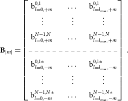
In Equation (11) $\textrm{b}_{l,\pm m}^{\textrm{i,j}}$
describes beam transfer coefficients for spherical harmonic order l increasing on a per-column-basis up to
$\textrm{b}_{l,\pm m}^{\textrm{i,j}}$
describes beam transfer coefficients for spherical harmonic order l increasing on a per-column-basis up to $l_{\textrm{max}}$
, (i, j) describes the baseline indices increasing on a per-row-basis until the maximum baseline configuration
$l_{\textrm{max}}$
, (i, j) describes the baseline indices increasing on a per-row-basis until the maximum baseline configuration $(N-1,N)$
has been reached. The matrix is split in half vertically with the upper half populating
$(N-1,N)$
has been reached. The matrix is split in half vertically with the upper half populating $+m$
and the bottom half populating
$+m$
and the bottom half populating $-m$
, where in the
$-m$
, where in the $-m$
section the coefficients have been conjugated to conform with definitions defined by Shaw et al. (Reference Shaw, Sigurdson, Pen, Stebbins and Sitwell2014). Lastly, the sky coefficients
$-m$
section the coefficients have been conjugated to conform with definitions defined by Shaw et al. (Reference Shaw, Sigurdson, Pen, Stebbins and Sitwell2014). Lastly, the sky coefficients $\textbf{a}$
(Equation 10) are only a function of
$\textbf{a}$
(Equation 10) are only a function of $+m$
, as due to the real-sky relation it satisfies that
$+m$
, as due to the real-sky relation it satisfies that $a_{l,m}=(\!-1)^{m}a_{l,-m}^{*}$
.
$a_{l,m}=(\!-1)^{m}a_{l,-m}^{*}$
.
Ideally, one would solve for $\textbf{a}$
through inverting Equation (10) by estimating the sky brightness temperatures using the visibilities, minimising
$\textbf{a}$
through inverting Equation (10) by estimating the sky brightness temperatures using the visibilities, minimising $||\textbf{v}-\textbf{B}\textbf{a}||^{2}$
(Shaw et al. Reference Shaw, Sigurdson, Pen, Stebbins and Sitwell2014; Eastwood et al. Reference Eastwood2018)
$||\textbf{v}-\textbf{B}\textbf{a}||^{2}$
(Shaw et al. Reference Shaw, Sigurdson, Pen, Stebbins and Sitwell2014; Eastwood et al. Reference Eastwood2018)
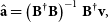 \begin{align} \hat{\textbf{a}} &= \left(\textbf{B}^{\dagger}\textbf{B}\right)^{-1}\textbf{B}^{\dagger}\textbf{v},\end{align}
where $\hat{\textbf{a}}$
is the estimate of
$\hat{\textbf{a}}$
is the estimate of $\textbf{a}$
; also known as the linear least-squares solution, where
$\textbf{a}$
; also known as the linear least-squares solution, where $\dagger$
denotes the conjugate transpose.
$\dagger$
denotes the conjugate transpose.
2.4. Spatial coverage
Eastwood et al. (Reference Eastwood2018) has shown that the maximum number of spherical harmonic orders $l_{\textrm{max}}$
that an interferometer is sensitive to is proportional to the array’s diameter. The maximum spherical harmonic order is given by
$l_{\textrm{max}}$
that an interferometer is sensitive to is proportional to the array’s diameter. The maximum spherical harmonic order is given by
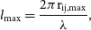 \begin{align} l_{\textrm{max}} &= \frac{2\pi\textrm{r}_{\textrm{ij},\textrm{max}}}{\lambda},\end{align}
where $\textrm{r}_{\textrm{ij},\textrm{max}}$
is the maximum baseline separation. We note that this is different to the original definition of Eastwood et al. (Reference Eastwood2018) by a factor of 2, as omitting this term causes the equation to no longer satisfy the Nyquist sampling rate required to represent the smallest variations across the sky measured by the longest baselines.
$\textrm{r}_{\textrm{ij},\textrm{max}}$
is the maximum baseline separation. We note that this is different to the original definition of Eastwood et al. (Reference Eastwood2018) by a factor of 2, as omitting this term causes the equation to no longer satisfy the Nyquist sampling rate required to represent the smallest variations across the sky measured by the longest baselines.
In standard radio interferometry the $u, v$
-plane coverage defines the spatial frequencies that have been measured by the array. Since in spherical harmonic transit interferometry the
$u, v$
-plane coverage defines the spatial frequencies that have been measured by the array. Since in spherical harmonic transit interferometry the $u, v$
-plane is omitted altogether, and a completely different coordinate system is used, one cannot sample the
$u, v$
-plane is omitted altogether, and a completely different coordinate system is used, one cannot sample the $u, v$
-plane to test for completeness. Consequently, an alternative formalism has to be employed to quantitatively describe the interferometer’s completeness of measurements in spherical harmonic l and m space.
$u, v$
-plane to test for completeness. Consequently, an alternative formalism has to be employed to quantitatively describe the interferometer’s completeness of measurements in spherical harmonic l and m space.
As explained in Subsection 2.3, the spherical harmonic coefficients of the beam-transfer functions can be used to visualise the spatial coverage information of the sky on a per-baseline basis (examples using EDA2 beam models and baselines are shown in Appendix A). Similar to $u, v$
-coverage, we combine the beam-transfer function coefficients
$u, v$
-coverage, we combine the beam-transfer function coefficients $b_{lm}$
from all baselines together:
$b_{lm}$
from all baselines together:
 \begin{align} {\mathcal{B}}_{lm} &= \sum\limits_{n=1}^{N}|b_{lm}^{n}|,\end{align}
where ${\mathcal{B}}_{lm}$
is the total spherical harmonic beam coverage (SHBC) contribution in spherical-harmonic space (SH-space) from all baselines for each l, m. This can be translated to percentage relative mode sensitivity in SH-space as:
${\mathcal{B}}_{lm}$
is the total spherical harmonic beam coverage (SHBC) contribution in spherical-harmonic space (SH-space) from all baselines for each l, m. This can be translated to percentage relative mode sensitivity in SH-space as:
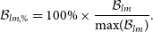 \begin{align} {\mathcal{B}}_{lm,\%} &= 100\%\times\frac{{\mathcal{B}}_{lm}}{\textrm{max}({\mathcal{B}}_{lm})}.\end{align}
An example of how this SH-space looks like is shown in Figure 2.
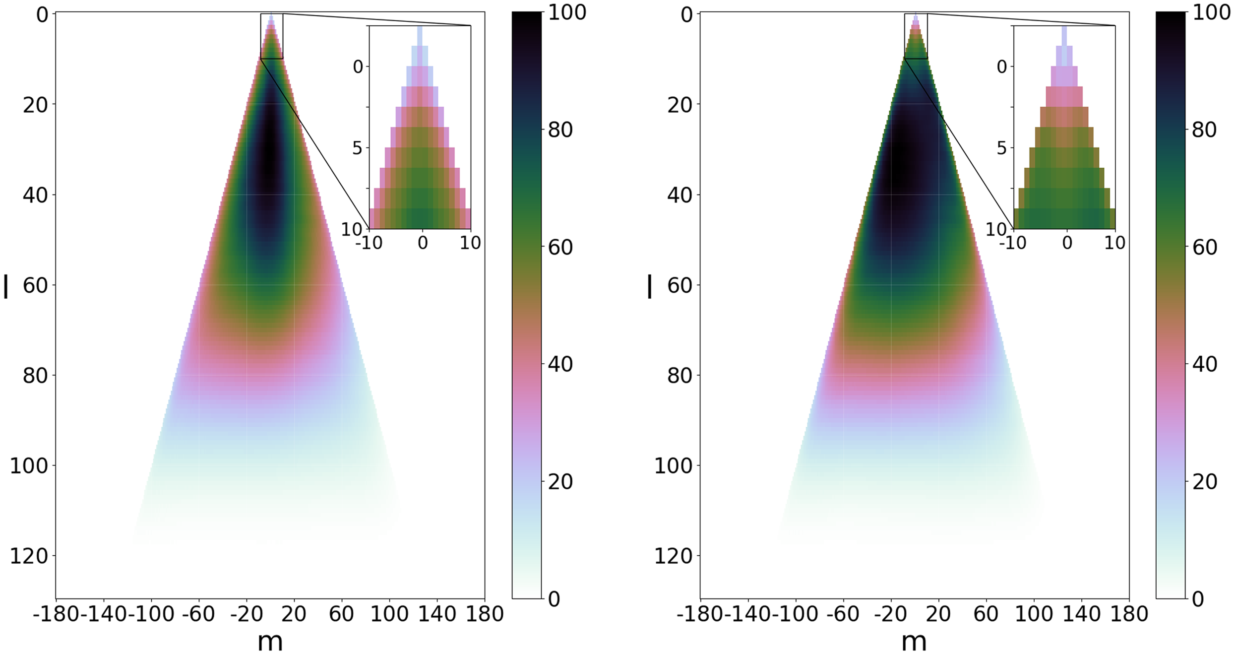
Figure 2. The spherical harmonic beam coverage, with contribution per mode in percentage relative mode sensitivity, in SH-space. A homogeneous array was assumed. The overall contribution is asymmetric in m due to the fact the beam transfer function is a complex waveform. This is a similar phenomenon one sees when plotting the $u, v$
-coverage in standard radio interferometry when the conjugate is not included. Left: x-polarisation, Right: y-polarisation. Zoomed areas show the first ten spherical harmonic beam coverage coefficient contributions.
$u, v$
-coverage in standard radio interferometry when the conjugate is not included. Left: x-polarisation, Right: y-polarisation. Zoomed areas show the first ten spherical harmonic beam coverage coefficient contributions.
Since these coefficients are weighting functions of the absolute spherical harmonic basis functions that operate across the full-sky, an equal (uniform) contribution of each SHBC mode in the SH-space coefficient plane would therefore result in a system that is ‘equisensitive’ to all spatial frequencies and phase components across the whole sky; that is the interferometer would measure the true sky. Such a uniform coverage would be equivalent to a complete $u, v$
-coverage for conventional interferometry. The SHBC can therefore be considered a powerful tool to visualise the interferometer’s coverage spherical harmonic coefficient space.
$u, v$
-coverage for conventional interferometry. The SHBC can therefore be considered a powerful tool to visualise the interferometer’s coverage spherical harmonic coefficient space.
2.5. Tikhonov-regularised $\mathrm{m}$
-modes
$\mathrm{m}$
-modes

In the general case telescopes cannot see some parts of the sky. As a result the square matrix $\textbf{B}^\dagger\textbf{B}$
is not full-rank and Equation (12) cannot be solved as
$\textbf{B}^\dagger\textbf{B}$
is not full-rank and Equation (12) cannot be solved as $\textbf{B}^\dagger\textbf{B}$
cannot be inverted.
$\textbf{B}^\dagger\textbf{B}$
cannot be inverted.
One way resolve this is to use either the Moore-Penrose pseudo-inverse or linear least squares (LLS) instead (Shaw et al. Reference Shaw, Sigurdson, Pen, Stebbins and Sitwell2014; Eastwood et al. Reference Eastwood2018). However, if the measurement data ( $\textbf{v}$
) is noise dominated or has too many unknowns, due to missing information on the sky, to fit the data properly, these methods might put emphasis on modes that vary on shorter timescales across the sky; suppressing the modes that vary on longer timescales instead (Eastwood et al. Reference Eastwood2018). This is because the conditions on which the pseudo-inverse and LLS satisfies the minimisation of the error and the estimated solution is only based on known information.
$\textbf{v}$
) is noise dominated or has too many unknowns, due to missing information on the sky, to fit the data properly, these methods might put emphasis on modes that vary on shorter timescales across the sky; suppressing the modes that vary on longer timescales instead (Eastwood et al. Reference Eastwood2018). This is because the conditions on which the pseudo-inverse and LLS satisfies the minimisation of the error and the estimated solution is only based on known information.
Conversely, Eastwood et al. (Reference Eastwood2018) proposed one could bias the known data by slightly increasing the initial error, but ultimately reducing the variance on what is being fit. This is also known as Tikhonov regularisation
 \begin{align} \hat{\textbf{a}} &= \left(\textbf{B}^{\dagger}\textbf{B}+\varepsilon\textbf{I}\right)^{-1}\textbf{B}^{\dagger}\textbf{v}\,,\end{align}
where $\varepsilon\ge0$
is the ridge-parameter and
$\varepsilon\ge0$
is the ridge-parameter and $\textbf{I}$
is the identity matrix; forcing
$\textbf{I}$
is the identity matrix; forcing $\varepsilon$
to 0 would again yield Equation (12). Equation (16) is also known as Tikhonov-regularised m-mode analysis (Eastwood et al. Reference Eastwood2018).
$\varepsilon$
to 0 would again yield Equation (12). Equation (16) is also known as Tikhonov-regularised m-mode analysis (Eastwood et al. Reference Eastwood2018).
2.6. Optimal ridge-parameter (
$\varepsilon$
) selection

Tikhonov regularisation regularises the data by forcing the matrix to be full rank by positively biasing $\textbf{B}$
on the diagonals enforcing preference for a solution where both
$\textbf{B}$
on the diagonals enforcing preference for a solution where both $||\textbf{v}-\textbf{B}\textbf{a}||^{2}$
and
$||\textbf{v}-\textbf{B}\textbf{a}||^{2}$
and $||\hat{\textbf{a}}||^{2}$
are jointly at their lowest possible norm (Eastwood et al. Reference Eastwood2018). In order to find a solution where both the 2-norm of the solution and the error are both at their minimum, an optimal value for
$||\hat{\textbf{a}}||^{2}$
are jointly at their lowest possible norm (Eastwood et al. Reference Eastwood2018). In order to find a solution where both the 2-norm of the solution and the error are both at their minimum, an optimal value for $\varepsilon$
has to be selected. To achieve this, Eastwood et al. (Reference Eastwood2018) suggested the use of L-curves as a graphical tool for determining the optimal solution for
$\varepsilon$
has to be selected. To achieve this, Eastwood et al. (Reference Eastwood2018) suggested the use of L-curves as a graphical tool for determining the optimal solution for $\varepsilon$
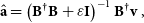
. In this case a graph plotting the norm of the solution against the norm of the residual error provides a characteristic L-shape with the minimum of both norms at the ‘elbow’ or ‘knee’ (Figure 3). Contrary to (Eastwood et al. Reference Eastwood2018), however, we decided to follow the definition by Hansen (Reference Hansen2001) instead. Here the L-curve is defined as a log-log graph with the axes inverted relative to Eastwood et al. (Reference Eastwood2018). This allows for steeper transitions outside the optimum region and a better distinction of the ‘knee’.
$\varepsilon$
. In this case a graph plotting the norm of the solution against the norm of the residual error provides a characteristic L-shape with the minimum of both norms at the ‘elbow’ or ‘knee’ (Figure 3). Contrary to (Eastwood et al. Reference Eastwood2018), however, we decided to follow the definition by Hansen (Reference Hansen2001) instead. Here the L-curve is defined as a log-log graph with the axes inverted relative to Eastwood et al. (Reference Eastwood2018). This allows for steeper transitions outside the optimum region and a better distinction of the ‘knee’.
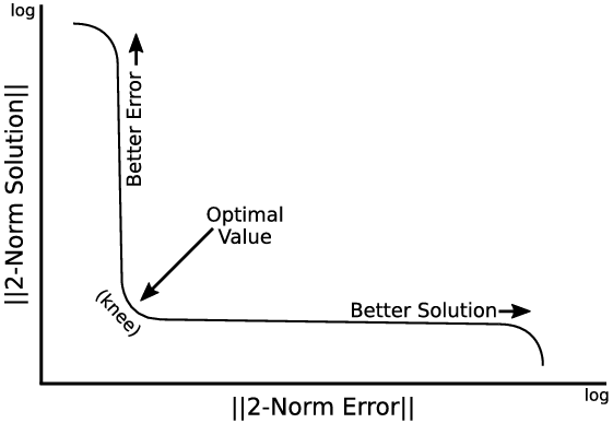
Figure 3. Example of an L-curve measurement plot in log-log space, the ‘knee’ indicates the optimal ridge regression value.
2.7. Prior knowledge to constrain the ridge parameter
In case one has prior knowledge of the sky, Eastwood et al. (Reference Eastwood2018) has shown that coefficients of a prior map can be used to better minimise for the estimated sky coefficients $\hat{\textbf{a}}$
, such that
$\hat{\textbf{a}}$
, such that $||\hat{\textbf{a}}-\textbf{a}_{\textrm{prior}}||$
is used instead and the solution is estimated by
$||\hat{\textbf{a}}-\textbf{a}_{\textrm{prior}}||$
is used instead and the solution is estimated by
 \begin{align} \hat{\textbf{a}} &= \left(\textbf{B}^{\dagger}\textbf{B}+\varepsilon\textbf{I}\right)^{-1}\textbf{B}^{\dagger}\left(\textbf{v}-\textbf{B}\textbf{a}_{\textrm{prior}}\right) + \textbf{a}_{\textrm{prior}}.\end{align}
However, this assumption is only valid if the prior coefficients have similar magnitudes to the coefficients of the measured sky. In our experience having a too large difference between the measured and model monopole component $a_{00}$
resulted in instability of the system and in improper constraints on the
$a_{00}$
resulted in instability of the system and in improper constraints on the $a_{00}$
mode. Because of this we’ve opted to constrain our measured modes with a prior where
$a_{00}$
mode. Because of this we’ve opted to constrain our measured modes with a prior where $\textrm{a}_{00}$
is subtracted. The global component can then be re-inserted after the regression step, such that
$\textrm{a}_{00}$
is subtracted. The global component can then be re-inserted after the regression step, such that
 \begin{align} \hat{\textbf{a}} &= \left(\textbf{B}^{\dagger}\textbf{B}+\varepsilon\textbf{I}\right)^{-1}\textbf{B}^{\dagger}\left(\textbf{v}-\textbf{B}\left[\textbf{a}_{\textrm{prior}}-a_{00}\right]\right) + \textbf{a}_{\textrm{prior}}.\end{align}
To determine the system’s insensitivity to specific modes in SH-space, the SHBC should be inspected. We note that this issue is a weakness of this form of regularisation as it disproportionately affects the cost function underlying the regularisation process for coefficients with large relative magnitude, for example, the monopole and dipole components for a low-frequency all-sky map.
3. Methods and data
In order to observe the Southern sky at low frequencies with the m-mode formalism, the EDA2 has been used.
3.1. The engineering development array 2
The EDA2, located at the Murchison Radio-astronomy Observatory (MRO) in Western Australia and a successor to the Engineering Development Array (EDA) (Wayth et al. Reference Wayth2017), is a 256-element dipole interferometer array (Wayth et al. Reference Wayth2021). The antenna elements are identical to the bow-tie dipole elements used in the Murchison Widefield Array (MWA) (Tingay et al. Reference Tingay2013), but distributed in a pseudo-random configuration spanning 35 m in diameter; much similar to what a station of the future SKA will look like. Each antenna is a dual-polarised antenna, allowing the EDA2 to measure a total of 512 signal paths. The EDA2 has a frequency range in accordance with the SKA-low specification of 50–350 MHz. Different to both the MWA and EDA, the EDA2 is not beamformed in analog domain, but instead digitised on a per-antenna basis. This allows the EDA2 to be run as a station beamformer, or as a small 256-element interferometer, which is the mode used for this paper.
3.2. Data and calibration
For this paper, we use two data sets spanning each between 25–28 h continuous zenith-pointed drift-scan observations. These two observations were separated by 7 months to have enough spatial separation of the sun between both observations for easier removal. The first observation was performed from September 2019 16-05:35:19 until September 2019 17-09:37:10 in Coordinated Universal Time (UTC), the second observation was performed from April 2020 10-11:30:10 until April 2020 11-12:17:36 in UTC.
The integration time for these observations was 1.98181 s. The observations were then averaged four times into a time-resolution of 7.92724 s and stored in sets of 12, containing 95.1269 s per file. To fulfil the sidereal day periodicity discussed in Section 2.3, 906 consecutive data files were selected to encompass a full sidereal day per observation. For this paper a single 0.926 MHz band at 159.375 MHz (centre band) was selected to generate a Southern sky image, since this band has very little interference.
The EDA2 is phase stable for days, so a single calibration is applied for each dataset. We use the Sun as a strong compact radio source with known flux density. The quiet sun has well measured radio flux density over a large frequency range (Benz Reference Benz2009), and we use this to define the flux density of the quiet sun to be 56 195 Jy for these observations at 159.375 MHz. The data were taken during solar minimum, hence the quiet sun model is appropriate. The calibration method used in this work has already been demonstrated by Sokolowski et al. (Reference Sokolowski2021), Wayth et al. (Reference Wayth2021) for science and system verification purposes.
Phase and amplitude calibration was performed during a 10-min interval centred on solar transit for each dataset, using an arbitrarily chosen antenna in the array as a reference, and discarding baselines shorter than $5\lambda$
to avoid bias from Galactic emission. The X and Y polarisations were independently calibrated. The solutions were transferred to the entire dataset.
$5\lambda$
to avoid bias from Galactic emission. The X and Y polarisations were independently calibrated. The solutions were transferred to the entire dataset.
The flux scale was corrected for the Sun’s location in the FEKOFootnote b-generated dipole radiation power pattern (Ung Reference Ung2019),Footnote c which is different for X (Figure 4) and Y (Figure 5) and is different for the two datasets because the Sun was at different declinations. The apparent flux density of the sun is reduced away from the peak directivity of the antenna (zenith in this case), hence we scale the data by factors of 0.856 and 0.624 for the X and Y dipoles respectively in September, and 0.780 and 0.481 for the X and Y dipoles respectively in April. Although the m-mode method can in principle embed different beam patterns for the elements in the array, the EDA2 patterns are very similar. Jones & Wayth (Reference Jones and Wayth2021) have shown that a single element beam model for the whole array is sufficient for better than 1% accuracy. As such, all elements are assumed to have the same beam patterns for their corresponding polarisations and have been normalised to be unity at their maxima.
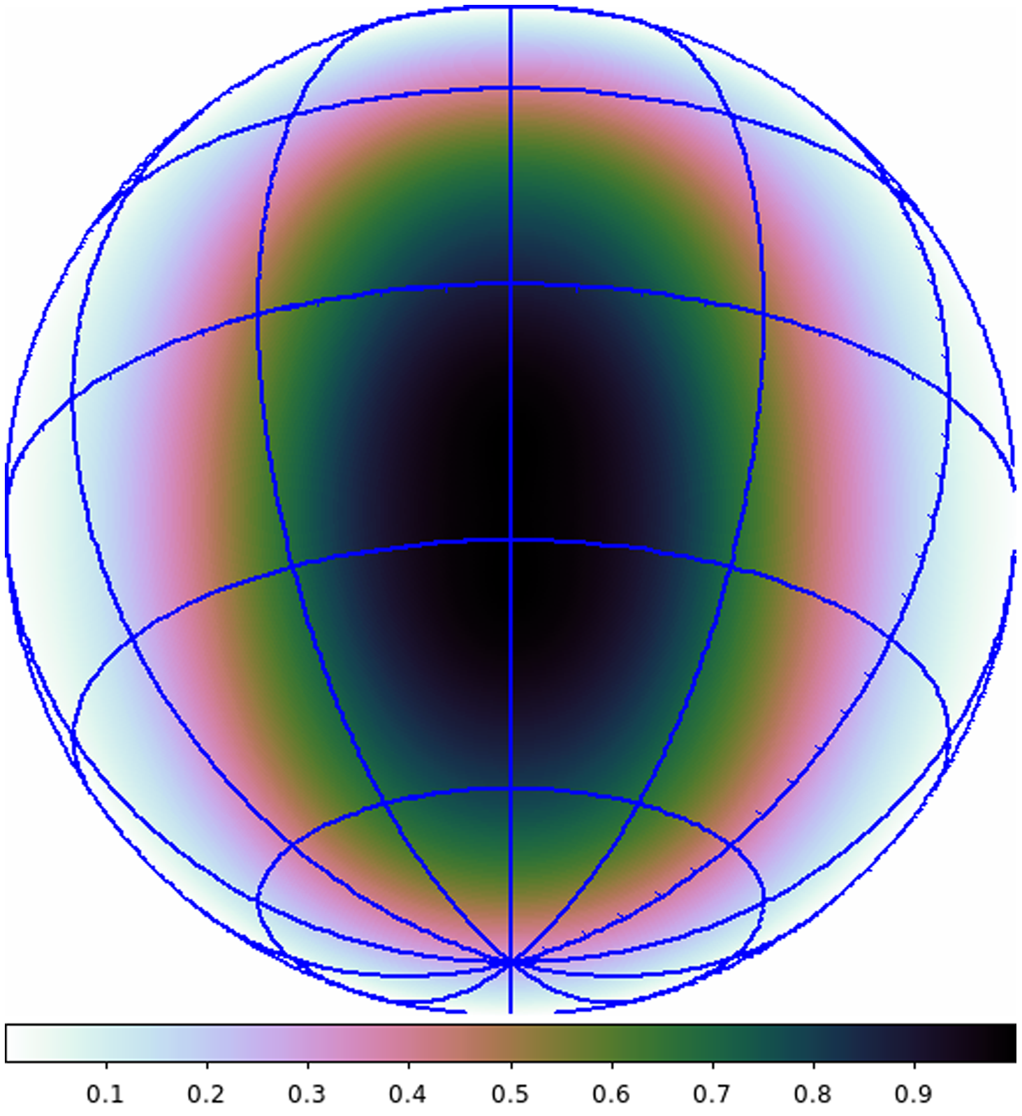
Figure 4. Normalised x-polarisation FEKO-simulated single-element beam pattern of the EDA2; orthographic projection on a hemisphere.
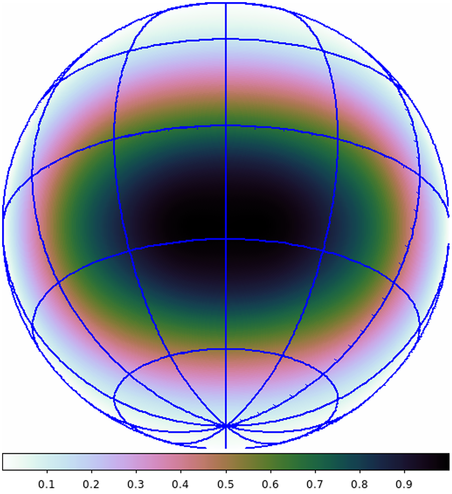
Figure 5. Normalised y-polarisation FEKO-simulated single-element beam pattern of the EDA2; orthographic projection on a hemisphere.
During commissioning work for EDA2, an additional temperature-dependent gain amplitude variation was found as described in Wayth et al. (Reference Wayth2021). This effect modulates the gain amplitude by approximately +/– 10% over a solar day. We use an identical procedure to model and correct for this variation as described in Wayth et al. (Reference Wayth2021).
To ensure we do not include bad data in our imaging phase, we flag timestamps where anomalies occur. In order to ascertain we do not void the periodicity assumption in Subsection 2.3, we flag the full 24-h observation for a baseline if flagging results in gaps in the observations spanning more than our angular resolution on the sky (in our case 12 min). If antennas consistently misbehave we remove all observations using this antenna from our imaging process. During the observations, 42 and 56 antennas were offline or flagged in the September and April data respectively, and are depicted in Figure 6.

Figure 6. EDA2 array 256 element layout in local (North-South, East-West) coordinates.
3.3. Spherical harmonic beam coverage
The SHBC in SH-space has been generated for both the X-polarisation and Y-polarisation and are depicted in Figure 2. From the beam coverage plots three observations can be made.
Firstly, due to our array diameter being limited to 35 m, we lack sensitivity in the higher l-modes. As can be seen, sensitivity is limited to a maximum of $l\approx 117$
and the drop-off from our higher modes to zero is quite steep.
$l\approx 117$
and the drop-off from our higher modes to zero is quite steep.
Secondly, when looking at the coefficient contribution across the first 10 spherical harmonic orders l, it can be seen that we have partial sensitivity at the lower orders, with 19% coverage on the $l=0$
mode. This is significant as this shows the m-mode formalism allows recovery on scales we would not be sensitive to with traditional snapshot imaging methods. Besides avoiding regridding artefacts in our imaging step, this is one of the primary advantages of spherical harmonic transit interferometry over the traditional method when it comes to diffuse all-sky imaging.
$l=0$
mode. This is significant as this shows the m-mode formalism allows recovery on scales we would not be sensitive to with traditional snapshot imaging methods. Besides avoiding regridding artefacts in our imaging step, this is one of the primary advantages of spherical harmonic transit interferometry over the traditional method when it comes to diffuse all-sky imaging.
In contrast, with traditional interferometric snapshot imaging we expect to be limited to scales corresponding 1 $\lambda$
, or approximately
$\lambda$
, or approximately $60^{\circ}$
in angular resolution, which is equivalent to a lowest mode sensitivity of
$60^{\circ}$
in angular resolution, which is equivalent to a lowest mode sensitivity of $l=5$
in spherical harmonic imaging. We verified this by calculating
$l=5$
in spherical harmonic imaging. We verified this by calculating $l_{\textrm{min}}$
for a single snapshot of the sky, which is achieved by substituting
$l_{\textrm{min}}$
for a single snapshot of the sky, which is achieved by substituting $\textrm{r}_{\textrm{ij},\textrm{max}}$
with
$\textrm{r}_{\textrm{ij},\textrm{max}}$
with $\textrm{r}_{\textrm{ij},\textrm{min}}$
(in our case approximately 1.5 m) in Equation (13).
$\textrm{r}_{\textrm{ij},\textrm{min}}$
(in our case approximately 1.5 m) in Equation (13).
Thirdly, the overall contribution is asymmetric in m. This is due to the fact the beam transfer function is a complex waveform that interacts with the conjugated complex spherical harmonic basis functions. During decomposition (depending on baseline vector orientation) the coefficients will shift either to positive or negative rank m in baselines that have East-West contributions. The same asymmetry is also encoded into the m-modes and will resolve itself when generating the coefficients of the real-valued sky, which are a product of $|m|$
. This is a similar phenomenon one sees when plotting the
$|m|$
. This is a similar phenomenon one sees when plotting the $u, v$
-coverage in standard radio interferometry when the conjugate is not included.
$u, v$
-coverage in standard radio interferometry when the conjugate is not included.
3.4. Ionosphere
In the operating bandwidth of the EDA2 (50–350 MHz) the spatial offsets caused by ionospheric effects is measured to be in the order of arcminutes (Jordan et al. Reference Jordan2017). Since the angular resolution of the EDA2 at 159 MHz is approximately $3^{\circ}$
, ionospheric offsets are negligible.
$3^{\circ}$
, ionospheric offsets are negligible.
3.5. Scintillation and refraction
Eastwood et al. (Reference Eastwood2018) has shown that scintillation and refraction offsets decrease when frequency increases, where these effects reduced to <5% at 73.152 MHz. Since we observe the sky at 159 MHz we assume these effects negligible and therefore do not consider them in our sky map imaging process. In addition, no scintillation was observed in snapshot images made from our data.
3.6. Coordinate system and pixel grid
For our coordinate system, we have opted to format all sky maps in the Hierarchical Equal Area isoLatitude Pixelation of a sphere (HEALPix)Footnote d (Gorski et al. Reference Gorski, Hivon, Banday, Wandelt, Hansen, Reinecke and Bartelmann2005), as this is an equal-area representation and naturally works with spherical harmonics.
Although HEALPix is convenient for correctly depicting discretely sampled functions on a sphere, it should be taken into account that the resolution of a HEALPix grid is dictated by its N $_{side}$
(i.e., the number of times a base pixel is divided along its sides) which operates in a power of 2 fashion. Ideally, based on our physical system dimensions our N
$_{side}$
(i.e., the number of times a base pixel is divided along its sides) which operates in a power of 2 fashion. Ideally, based on our physical system dimensions our N $_{side}$
would be defined as
$_{side}$
would be defined as
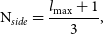 \begin{align} \textrm{N}_{side} &= \frac{l_{\textrm{max}}+1}{3},\end{align}
which in our case with a maximum diameter of 35 m and a frequency of 159 MHz would result in an N $_{side}$
of 39. However, since this is not a power of 2, our real N
$_{side}$
of 39. However, since this is not a power of 2, our real N $_{side}$
needs to be increased to the nearest power of 2; which is N
$_{side}$
needs to be increased to the nearest power of 2; which is N $_{side}=64$
; resulting in a pixel area of
$_{side}=64$
; resulting in a pixel area of $\sim 0.84$
square degrees.
$\sim 0.84$
square degrees.
3.7. Sky coefficients
In order to retrieve the spherical harmonic sky coefficients $(\textbf{a})$
to generate images of the Southern sky, we have to solve for Equation (16). The beam function
$(\textbf{a})$
to generate images of the Southern sky, we have to solve for Equation (16). The beam function $\textbf{B}$
is generated by multiplying the individual x-pol and y-pol beam models with the respective fringes on the sky for each baseline. The fringes are calculated by solving for the exponent in Equation (1) on the whole sky.
$\textbf{B}$
is generated by multiplying the individual x-pol and y-pol beam models with the respective fringes on the sky for each baseline. The fringes are calculated by solving for the exponent in Equation (1) on the whole sky.
Instead of inverting $\textbf{B}$
as block-diagonal matrix,
$\textbf{B}$
as block-diagonal matrix, $\textbf{B}$
is split in blocks of independent m’s (
$\textbf{B}$
is split in blocks of independent m’s ( $\textbf{B}_{m}$
), where each block is defined as in Equation (11); to reduce size of matrices required in computer memory. Since the m-modes are grouped on an m-by-m basis, we can invert each m-mode and
$\textbf{B}_{m}$
), where each block is defined as in Equation (11); to reduce size of matrices required in computer memory. Since the m-modes are grouped on an m-by-m basis, we can invert each m-mode and $\textbf{B}_{m}$
matrix independently to solve for each individual
$\textbf{B}_{m}$
matrix independently to solve for each individual $\hat{a}_{m}$
. However, given that our shortest baseline separation (1.5 m) at 159 MHz is not much shorter than our wavelength (
$\hat{a}_{m}$
. However, given that our shortest baseline separation (1.5 m) at 159 MHz is not much shorter than our wavelength ( $\lambda=1.89\,$
m), we are no longer fully sensitive to the lowest spherical harmonic orders and global signal component (
$\lambda=1.89\,$
m), we are no longer fully sensitive to the lowest spherical harmonic orders and global signal component ( $\hat{a}_{0,0}$
); as shown in Figure 2. Therefore, we need a prior model to better fit for the solutions of
$\hat{a}_{0,0}$
); as shown in Figure 2. Therefore, we need a prior model to better fit for the solutions of $\hat{\textbf{a}}$
.
$\hat{\textbf{a}}$
.
3.7.1. Prior model
In order to properly regularise for diffuse emission in the sky map, Equation (17) will be used instead. The model used as prior information is the desourced, destriped Haslam map from Remazeilles et al. (Reference Remazeilles, Dickinson, Banday, Bigot-Sazy and Ghosh2015). Since the Haslam map itself is at 408 MHz, the map has been rescaled to match the correct brightness temperature using pyGDSM (Price Reference Price2016), a python interface for diffuse global sky models spectral indices (SI) for downscaling to 159 MHz are embedded in the package and, for the Haslam map, extracted from Mozdzen et al. (Reference Mozdzen, Bowman, Monsalve and Rogers2016). We’ve selected Haslam as our prior as it is still the most prevalent in use; furthermore, in most sky map papers it’s a common approach to compute SI between a single sky map frequency and the 408 MHz Haslam map. This should provide others a reference frame to compare their maps to our prior constrained map and map without prior.
The map is also downscaled to the correct HEALPix N $_{side}$
in order to match our measurements and angular resolution. Additionally, we employed a Gaussian smoothing kernel at the full-width half-maximum (FWHM) of our synthesised beam. This is achieved by applying HEALPix’s ud_grade() and smoothing() functions respectively; in the case of changing pixel scale, HEALPix sets the rescaled superpixel to be the mean of the children pixels. The resulting model map is shown in Figure 7. We also need to account for the brightness of the sun in both the September and April observations, the model map is used to create two prior maps for Equation (18) with a model of the sun at the correct location in the sky for both observations. We opted only to remove the global component as the discrepancy between
$_{side}$
in order to match our measurements and angular resolution. Additionally, we employed a Gaussian smoothing kernel at the full-width half-maximum (FWHM) of our synthesised beam. This is achieved by applying HEALPix’s ud_grade() and smoothing() functions respectively; in the case of changing pixel scale, HEALPix sets the rescaled superpixel to be the mean of the children pixels. The resulting model map is shown in Figure 7. We also need to account for the brightness of the sun in both the September and April observations, the model map is used to create two prior maps for Equation (18) with a model of the sun at the correct location in the sky for both observations. We opted only to remove the global component as the discrepancy between $a_{00}$
on the prior and the measured sky was too large. This mode has later been reinserted to assure a global sky component is present in the maps. These model map coefficients are calculated in accordance to Equation (6).
$a_{00}$
on the prior and the measured sky was too large. This mode has later been reinserted to assure a global sky component is present in the maps. These model map coefficients are calculated in accordance to Equation (6).

Figure 7. 159 MHz diffuse model map, log-scaling (N $_{side}=64$
). Generated from the 2014 desourced and destriped reprocessed 408 MHz Haslam map (Remazeilles et al. Reference Remazeilles, Dickinson, Banday, Bigot-Sazy and Ghosh2015).
$_{side}=64$
). Generated from the 2014 desourced and destriped reprocessed 408 MHz Haslam map (Remazeilles et al. Reference Remazeilles, Dickinson, Banday, Bigot-Sazy and Ghosh2015).
3.7.2. Ridge parameter selection
In order to properly constrain the inversion of the m-modes to solve for the sky $\hat{\textbf{a}}$
, we need to determine the proper value for
$\hat{\textbf{a}}$
, we need to determine the proper value for $\varepsilon$
given the measured data. Since we have two 24h observations, each with two polarisations, four ridge parameters have to be selected. Since solving for
$\varepsilon$
given the measured data. Since we have two 24h observations, each with two polarisations, four ridge parameters have to be selected. Since solving for $\varepsilon$
requires us to solve for the norms of the error and the solution multiple times to determine the optimal value.
$\varepsilon$
requires us to solve for the norms of the error and the solution multiple times to determine the optimal value.
To select the $\varepsilon$
to best fit our data, ideally one would like to sample for as many values for
$\varepsilon$
to best fit our data, ideally one would like to sample for as many values for $\varepsilon$
as possible; preferably infinite. However, due to the computational complexity of solving for Equation (18), choosing for an increasingly large sample of
$\varepsilon$
as possible; preferably infinite. However, due to the computational complexity of solving for Equation (18), choosing for an increasingly large sample of $\varepsilon$
quickly becomes a non-feasible endeavour; a clear trade-off exists between time spent to constrain
$\varepsilon$
quickly becomes a non-feasible endeavour; a clear trade-off exists between time spent to constrain $\varepsilon$
and the accuracy that we gain from it. To reduce the time spent, but still maintain accuracy, we propose an alternate method to constrain
$\varepsilon$
and the accuracy that we gain from it. To reduce the time spent, but still maintain accuracy, we propose an alternate method to constrain $\varepsilon$
instead; a two-stage constraining scenario has been created to ease computational strain and time-constraints. Finely sampling for a reduced subset of a full array, yet with still sufficient SHBC in SH-space, provides us a rough estimation where the optimum must lie for the full array. Coarsely recalculating
$\varepsilon$
instead; a two-stage constraining scenario has been created to ease computational strain and time-constraints. Finely sampling for a reduced subset of a full array, yet with still sufficient SHBC in SH-space, provides us a rough estimation where the optimum must lie for the full array. Coarsely recalculating $\varepsilon$
across this sample-space for the full array will give us a close estimate for the best overall fit. Tweaking the recalculated
$\varepsilon$
across this sample-space for the full array will give us a close estimate for the best overall fit. Tweaking the recalculated $\varepsilon$
around this close estimate should therefore yield us our optimal solution.
$\varepsilon$
around this close estimate should therefore yield us our optimal solution.
For the EDA2 array subset, to make sure we still maintain a proper baseline distribution, only the outer rings of elements have been selected for the first stage (Figure 8). To determine the rough optimal range of $\varepsilon$
for this subset, a fine-scale inversion process of Equation (17) is ran 2 000 times for each observation and each polarisation, minimising for
$\varepsilon$
for this subset, a fine-scale inversion process of Equation (17) is ran 2 000 times for each observation and each polarisation, minimising for $||\textbf{v}-\textbf{B}\hat{\textbf{a}}||$
and
$||\textbf{v}-\textbf{B}\hat{\textbf{a}}||$
and $||\hat{\textbf{a}}-\textbf{a}_{\textrm{prior}}||$
each time. The resulting L-curves are shown in Figure 9, which represent the L-curve from the ‘knee’ down. The optimal
$||\hat{\textbf{a}}-\textbf{a}_{\textrm{prior}}||$
each time. The resulting L-curves are shown in Figure 9, which represent the L-curve from the ‘knee’ down. The optimal $\varepsilon$
values resulting from the L-curves are
$\varepsilon$
values resulting from the L-curves are $\varepsilon_{32}=0.006$
for the 32-element data.
$\varepsilon_{32}=0.006$
for the 32-element data.
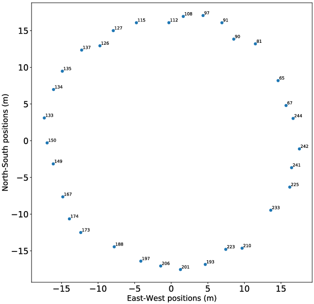
Figure 8. EDA2 array 32 element outer ring layout in local (North-South, East-West) coordinates.
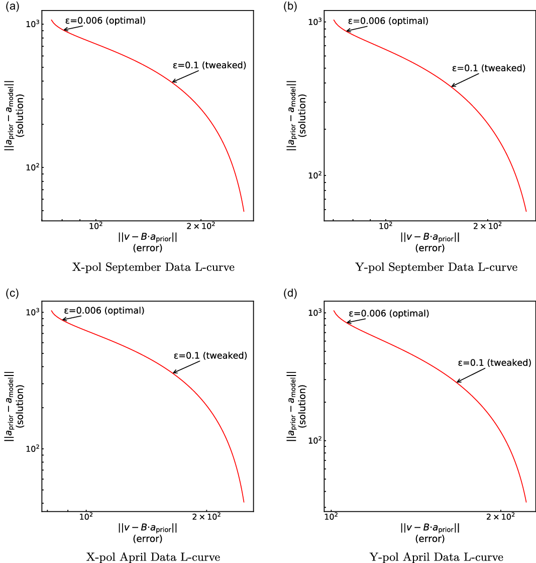
Figure 9. L-curves computed for the EDA2 data for both September and April observations; and X and Y polarisations. The data was generated by first trialing 2 000 samples of $\varepsilon$
for a 32-element subset array (
$\varepsilon$
for a 32-element subset array ( $\varepsilon_{32}$
) and then fit for the full array by coarsely re-sampling at 20 evenly spaced points within the linear regime in the 32-element L-curve. The final
$\varepsilon_{32}$
) and then fit for the full array by coarsely re-sampling at 20 evenly spaced points within the linear regime in the 32-element L-curve. The final $\varepsilon$
is then obtained tough tweaking around the best coarse fit for an optimum 256 element solution (
$\varepsilon$
is then obtained tough tweaking around the best coarse fit for an optimum 256 element solution ( $\varepsilon_{256}$
). The data is represented following Figure 3, where the 2 000 sample points generated an L-curve from the ‘knee’ down; that is, the bottom half of Figure 3 is therefore only shown in this representation.
$\varepsilon_{256}$
). The data is represented following Figure 3, where the 2 000 sample points generated an L-curve from the ‘knee’ down; that is, the bottom half of Figure 3 is therefore only shown in this representation.
In order to then better constrain $\varepsilon$
for the 256-element array, in the second stage the norms are recalculated for 20
$\varepsilon$
for the 256-element array, in the second stage the norms are recalculated for 20 $\varepsilon$
data points equidistantly spaced on the linear regime in the L-curves (between approximately 70 and 200 on the horizontal axis). For the lowest-norm outcomes in each polarisation, the
$\varepsilon$
data points equidistantly spaced on the linear regime in the L-curves (between approximately 70 and 200 on the horizontal axis). For the lowest-norm outcomes in each polarisation, the $\varepsilon$
are then tweaked to assure the lowest norms possible providing the best fit for the solutions of the data. The final
$\varepsilon$
are then tweaked to assure the lowest norms possible providing the best fit for the solutions of the data. The final $\varepsilon$
values obtained were the same for all polarisations and are
$\varepsilon$
values obtained were the same for all polarisations and are $\varepsilon_{256}=0.1$
.
$\varepsilon_{256}=0.1$
.
3.8. Deconvolution of compact sources
Since we have a finite array that physically limits the angular resolution and has incomplete sampling of the sky, much similar to holes in the $u, v$
-sampling space in traditional interferometry, we expect our sky sources to be convolved with a PSF. In order to counteract a PSF we can try to minimise their contribution through deconvolution, traditionally done via the CLEAN algorithm in radio astronomy (Thompson et al. Reference Thompson, Moran and Swenson George2017).
$u, v$
-sampling space in traditional interferometry, we expect our sky sources to be convolved with a PSF. In order to counteract a PSF we can try to minimise their contribution through deconvolution, traditionally done via the CLEAN algorithm in radio astronomy (Thompson et al. Reference Thompson, Moran and Swenson George2017).
Originally, CLEAN (Högbom Reference Högbom1974) was designed to work with Fourier-synthesis imaging methods. In spherical harmonic transit interferometry, we instead work in spherical harmonic domain and cannot directly apply standard CLEAN algorithms. Eastwood et al. (Reference Eastwood2018) showed how to directly relate the PSFs in spherical harmonic coefficient space:
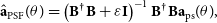 \begin{align} \hat{\textbf{a}}_{\textrm{PSF}}(\theta) &= \left(\textbf{B}^{\dagger}\textbf{B}+\varepsilon\textbf{I}\right)^{-1}\textbf{B}^{\dagger}\textbf{B}\textbf{a}_{\textrm{ps}}(\theta),\end{align}
where $\hat{\textbf{a}}_{\textrm{PSF}}$
are the spherical harmonic coefficients of the PSF, and
$\hat{\textbf{a}}_{\textrm{PSF}}$
are the spherical harmonic coefficients of the PSF, and $\textbf{a}_{\textrm{ps}}$
is the spherical harmonic decomposition of a single point on the sky.
$\textbf{a}_{\textrm{ps}}$
is the spherical harmonic decomposition of a single point on the sky.
As part of the proposed CLEANing algorithm by Eastwood et al. (Reference Eastwood2018), it was noted the PSFs are shift invariant in RA, that is, PSFs only have to be generated on a per-declination basis. Unlike Eastwood et al. (Reference Eastwood2018), instead of pre-identifying CLEAN components and precalcuting the PSFs for each of those components, we simply store a PSF image for each possible declination on the sky and do all deconvolution in image space. To deconvolve the ‘dirty images’, bright compact sources are selected and windowed in image space to determine the brightest pixel. For each bright pixel a PSF is selected based on declination and rotated to the correct longitude. We tested that each PSF generated via rotation was consistent with its equivalent PSF, generated via spherical harmonics for a point source, at that location. Residuals and imaging artefacts propagated by imaging the rotated PSFs are $<0.01\%$
and therefore considered negligible. Examples of these residuals are shown in Figure 10.
$<0.01\%$
and therefore considered negligible. Examples of these residuals are shown in Figure 10.
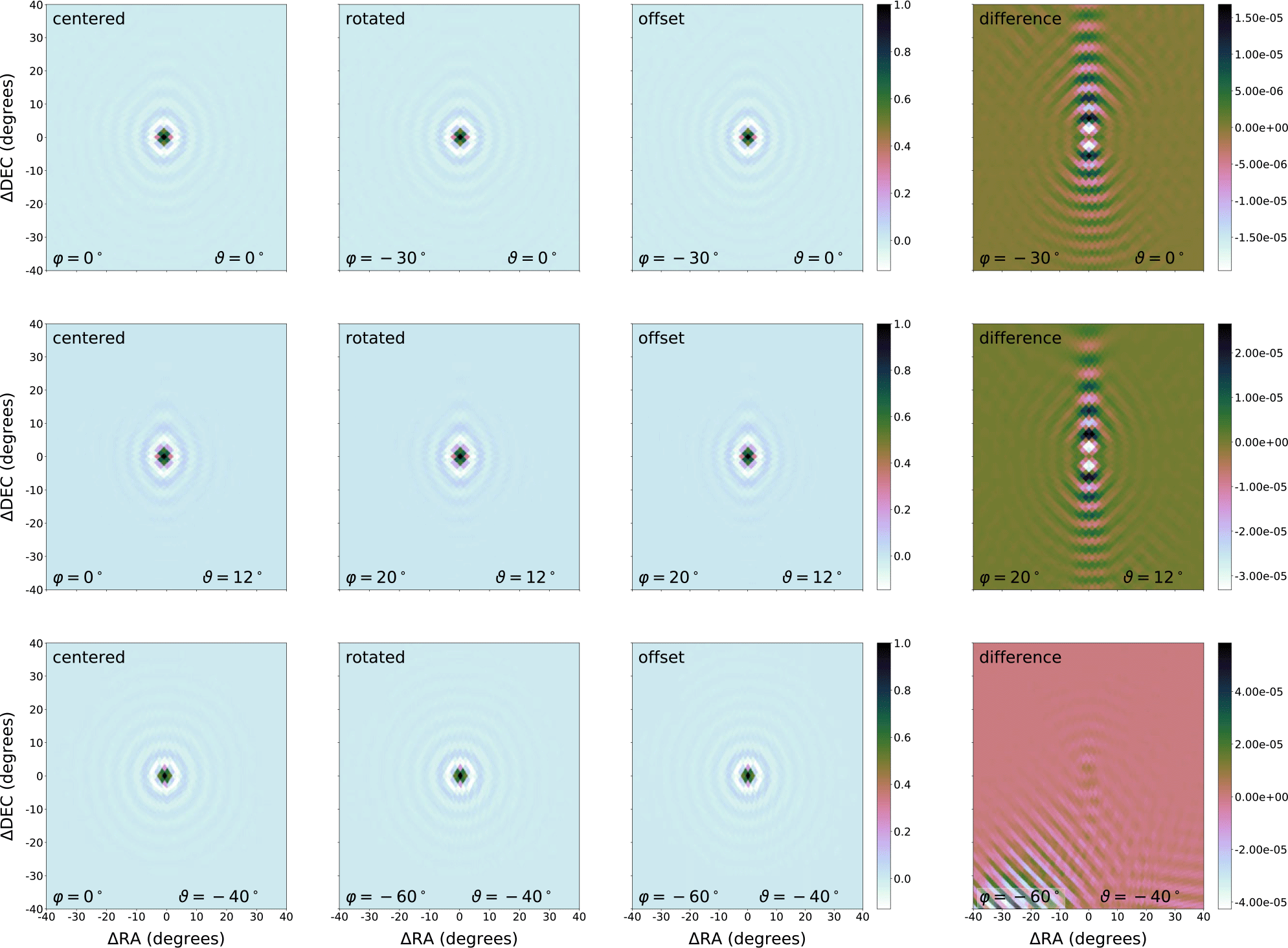
Figure 10. EDA2 array point-spread functions (PSFs) Left column: PSFs generated at an (RA) ( $\varphi$
) of 0 degrees, Middle left column: PSFs of the left column rotated in coefficient space to a specific RA, Middle right column: PSFs generated at an offset RA (
$\varphi$
) of 0 degrees, Middle left column: PSFs of the left column rotated in coefficient space to a specific RA, Middle right column: PSFs generated at an offset RA ( $\varphi$
), Right column: difference between the rotated and the offset PSFs. Top row: PSFs generated at a declination (DEC) (
$\varphi$
), Right column: difference between the rotated and the offset PSFs. Top row: PSFs generated at a declination (DEC) ( $\vartheta$
) of 0 degrees, Middle row: PSFs generated at a DEC (
$\vartheta$
) of 0 degrees, Middle row: PSFs generated at a DEC ( $\vartheta$
) of 12 degrees, Bottom row: PSFs generated at a DEC (
$\vartheta$
) of 12 degrees, Bottom row: PSFs generated at a DEC ( $\vartheta$
) of –40 degrees.
$\vartheta$
) of –40 degrees.
After deconvolving the PSFs, the identified pixels used to model the PSFs are then convolved with a restoring Gaussian (which is an identical Gaussian fit to the PSF central region to preserve the flux) and reinserted into the residual image to create the CLEANed sky map. It should be noted that this image-based CLEANing method closely follows the CLEAN steps outlined by Eastwood et al. (Reference Eastwood2018), however, deviates at the stages where PSFs selection and deconvolution occurs. The complete step-by-step selective image-based CLEANing process we employed is outlined below:
| Selective Image-based Spherical |
| Harmonic CLEANing process |
|


3.9. Source removal
3.9.1. The sun
The Sun in our images is very strong and slightly smeared out, meaning we cannot perfectly deconvolve the PSF from our images, leaving residual ripples into our sky maps. This has been the main motivation to image the sky during two different months (April and September) where the sun manifests at different locations on the sky. This gives us the opportunity to combine the two epochs such that the sun no longer is present. We achieve this by averaging the two sky maps together, after CLEANing, according to Figure 11. The blue region contains the September data, the red region contains the April data, and the green region is a linear-gradient weighted average of both maps; the green region closer to the red region contains more contribution from the April observations and vice versa. This action is performed on both x-polarisation and y-polarisation.
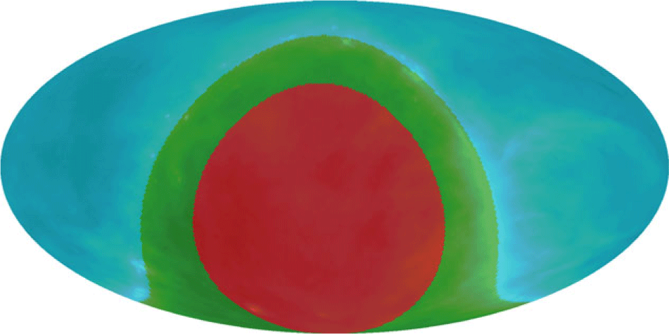
Figure 11. Contour map for combining the April and September data. Cyan: April data, Green: linearly-weighted combination of April and September data, Red: September data. Overlaid with the model map from Figure 7 as a reference for overlap of regions.
3.9.2. Field of view edge
Regions at the sky near the northern horizon are poorly sampled and passed through a low-sensitivity part of the beam. Although these regions of the sky do appear in our output images they are not trustworthy. Instead of truncating the sky at an arbitrary DEC, we apply difference weighting between the intensity map we generate using our observations, and the prior model (for the prior fit map) or global ( $a_{00}$
) emission (for the non-fit map) to provide a smoother transition towards the region of the sky no longer observable to the system. This has a small trade-off of sacrificing a small region of our measurable sky to better constrain the edges of our FoV. These regions are depicted in Figure 12, in the red region the intensity map is 100% represented, the green region is again a linear-gradient weighted average of both the intensity map and the model maps (Haslam/diffuse) between
$a_{00}$
) emission (for the non-fit map) to provide a smoother transition towards the region of the sky no longer observable to the system. This has a small trade-off of sacrificing a small region of our measurable sky to better constrain the edges of our FoV. These regions are depicted in Figure 12, in the red region the intensity map is 100% represented, the green region is again a linear-gradient weighted average of both the intensity map and the model maps (Haslam/diffuse) between $+50^{\circ}$
and
$+50^{\circ}$
and $+60^{\circ}$
; the green region closer to red denotes a higher contribution of the intensity map, whereas the green region near the cyan region has more weight on the model. The cyan region has solely contribution of the model map depicted in Figure 7 or the
$+60^{\circ}$
; the green region closer to red denotes a higher contribution of the intensity map, whereas the green region near the cyan region has more weight on the model. The cyan region has solely contribution of the model map depicted in Figure 7 or the $a_{00}$
diffuse mode map.
$a_{00}$
diffuse mode map.
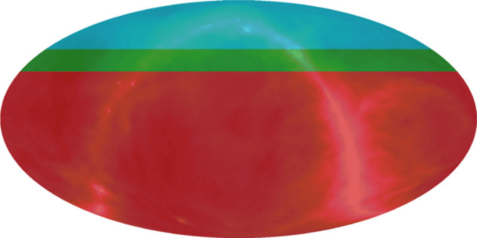
Figure 12. Contour map for combining the intensity map and model data. Cyan: model data, Green: linearly-weighted combination of intensity map and model data, Red: intensity map. Overlaid with the model map from Figure 7 as a reference for overlap of regions.
4. Results
The resulting EDA2 sky maps are presented in Figures 13 and 14. Two versions of sky maps are made, one without prior fitting (Figure 13) and one with the updated desourced and destriped Haslam map (Remazeilles et al. Reference Remazeilles, Dickinson, Banday, Bigot-Sazy and Ghosh2015) used as a prior (Figure 14). Both sky maps have been presented in equatorial coordinates as that is the coordinate system we measured the sky in. Versions of the sky maps in their default HEALPix representation, with coordinate grid, can be found in Appendix B. These maps have been created by combining two 24-h observations in different epochs (September and April) to be able to remove the Sun using Figure 11. Both maps have a resolution of approximately $3.1^{\circ}$
, supersampled to a
$3.1^{\circ}$
, supersampled to a $0.916^{\circ}$
(
$0.916^{\circ}$
( $0.84$
square degrees) pixel scale. The FWHM of the synthesised beam at
$0.84$
square degrees) pixel scale. The FWHM of the synthesised beam at $\delta=-40^{\circ}$
,
$\delta=-40^{\circ}$
, $\delta=0^{\circ}$
, and
$\delta=0^{\circ}$
, and $\delta=12^{\circ}$
are
$\delta=12^{\circ}$
are $3.10^{\circ}\times3.01^{\circ}$
,
$3.10^{\circ}\times3.01^{\circ}$
, $3.30^{\circ}\times3.06^{\circ}$
, and
$3.30^{\circ}\times3.06^{\circ}$
, and $3.71^{\circ}\times3.05^{\circ}$
respectively (major
$3.71^{\circ}\times3.05^{\circ}$
respectively (major $\times$
minor axis). These maps have been corrected for systematic and regression bias (Subsection 4.3) and common-mode noise has been removed (Subsection 4.1.1). The 159 MHz sky maps as well as a noise map and an SI map are accessible and available for download at PASA datastoreFootnote f and LAMBDAFootnote g.
$\times$
minor axis). These maps have been corrected for systematic and regression bias (Subsection 4.3) and common-mode noise has been removed (Subsection 4.1.1). The 159 MHz sky maps as well as a noise map and an SI map are accessible and available for download at PASA datastoreFootnote f and LAMBDAFootnote g.
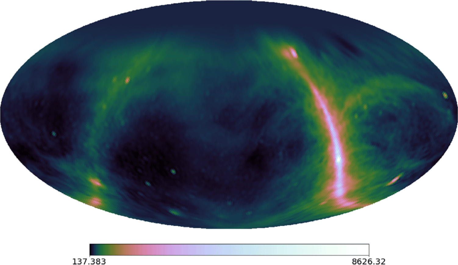
Figure 13. 159 MHz diffuse EDA2 map (equatorial view), log-scale. Generated without the use of a prior model, the global sky component is reinserted.
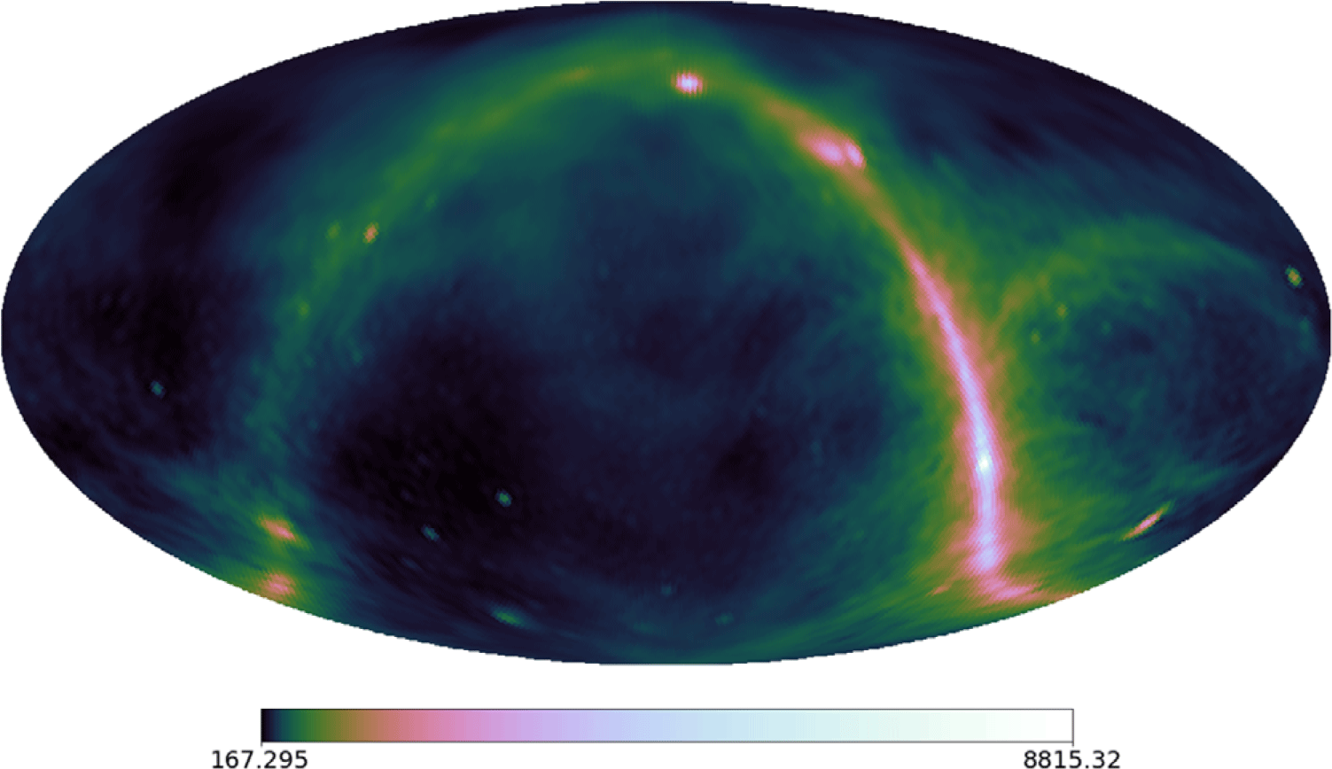
Figure 14. 159 MHz diffuse EDA2 map (equatorial view), log-scale. Generated with the use of a prior model to constrain the beam-inverse, the Northern hemisphere is therefore equivalent to the diffuse reprocessed Haslam map depicted in Figure 7.
4.1. Difference visibility dataset
We create a difference visibility dataset by averaging the subtracted odd and even non-averaged samples from each other within each one minute averaged visibility sample following Equation (21).
 \begin{align} \Delta\sigma_{\textrm{ij}} &= \sqrt{\frac{\sum\limits_{s=0}^{S_{\textrm{max}, \Delta \textrm{V}}/2}\frac{\left(V_{s,\Delta V}^{\textrm{ij}, \textrm{even}}-V_{s,\Delta V}^{\textrm{ij}, \textrm{odd}}\right)}{\sqrt{2}}\frac{\left(V_{s,\Delta V}^{\textrm{ij}, \textrm{even}}-V_{s,\Delta V}^{\textrm{ij}, \textrm{odd}}\right)^*}{\sqrt{2}}}{S_{\textrm{max}, \Delta \textrm{V}}/2}}.\end{align}
Here, $S_{\textrm{max}}$
is the maximum number of samples within a one minute averaged visibility sample (in our case eight),
$S_{\textrm{max}}$
is the maximum number of samples within a one minute averaged visibility sample (in our case eight), $V_{s,\Delta V}^{\textrm{ij}, \textrm{even}}$
and
$V_{s,\Delta V}^{\textrm{ij}, \textrm{even}}$
and $V_{s,\Delta V}^{\textrm{ij}, \textrm{odd}}$
describe the odd and even time samples for each 1 min average for sample point s at baseline (i, j) respectively, and
$V_{s,\Delta V}^{\textrm{ij}, \textrm{odd}}$
describe the odd and even time samples for each 1 min average for sample point s at baseline (i, j) respectively, and $\Delta\sigma_{\textrm{ij}}$
is the average visibility noise within average sample. Each difference visibility noise sample is then averaged together to within the same one-minute average bin. We use this dataset to estimate the noise in our sky maps as well as correct for any common-mode noise that occurs.
$\Delta\sigma_{\textrm{ij}}$
is the average visibility noise within average sample. Each difference visibility noise sample is then averaged together to within the same one-minute average bin. We use this dataset to estimate the noise in our sky maps as well as correct for any common-mode noise that occurs.
4.1.1. Noise correction
Eastwood et al. (Reference Eastwood2018) has shown that radio frequency interference (RFI) from sources that do not follow the rotation of the sky, or that common-mode pickup between interferometer elements can generate unwanted contribution to the visibilities. This will smear out across RA in image space, manifesting as concentric rings at various declinations across the sky. To see these effects in the EDA2 sky maps we used the difference visibility dataset.
To get an image representation of the noise, the noise samples are inserted in our m-mode imaging pipeline with equal settings as to imaging the measured sky. This operation is performed for both X and Y polarisations for the April and September data. The resulting noise images are shown in Figure 15. It is evident that similar to Eastwood et al. (Reference Eastwood2018) we also have concentric rings at varying DEC, that correspond to modes of $m\leq1$
. For noise to smear out like this on the sky the source has to be common across all elements or stationary in nature relative to the array, likely this is therefore a product of terrestrial noise or common-mode pickup interfering with our 24 h observation’s signal path. These noise artefacts range from
$m\leq1$
. For noise to smear out like this on the sky the source has to be common across all elements or stationary in nature relative to the array, likely this is therefore a product of terrestrial noise or common-mode pickup interfering with our 24 h observation’s signal path. These noise artefacts range from $-7.7$
to 2.6 K and hence are small relative to our sky signal.
$-7.7$
to 2.6 K and hence are small relative to our sky signal.
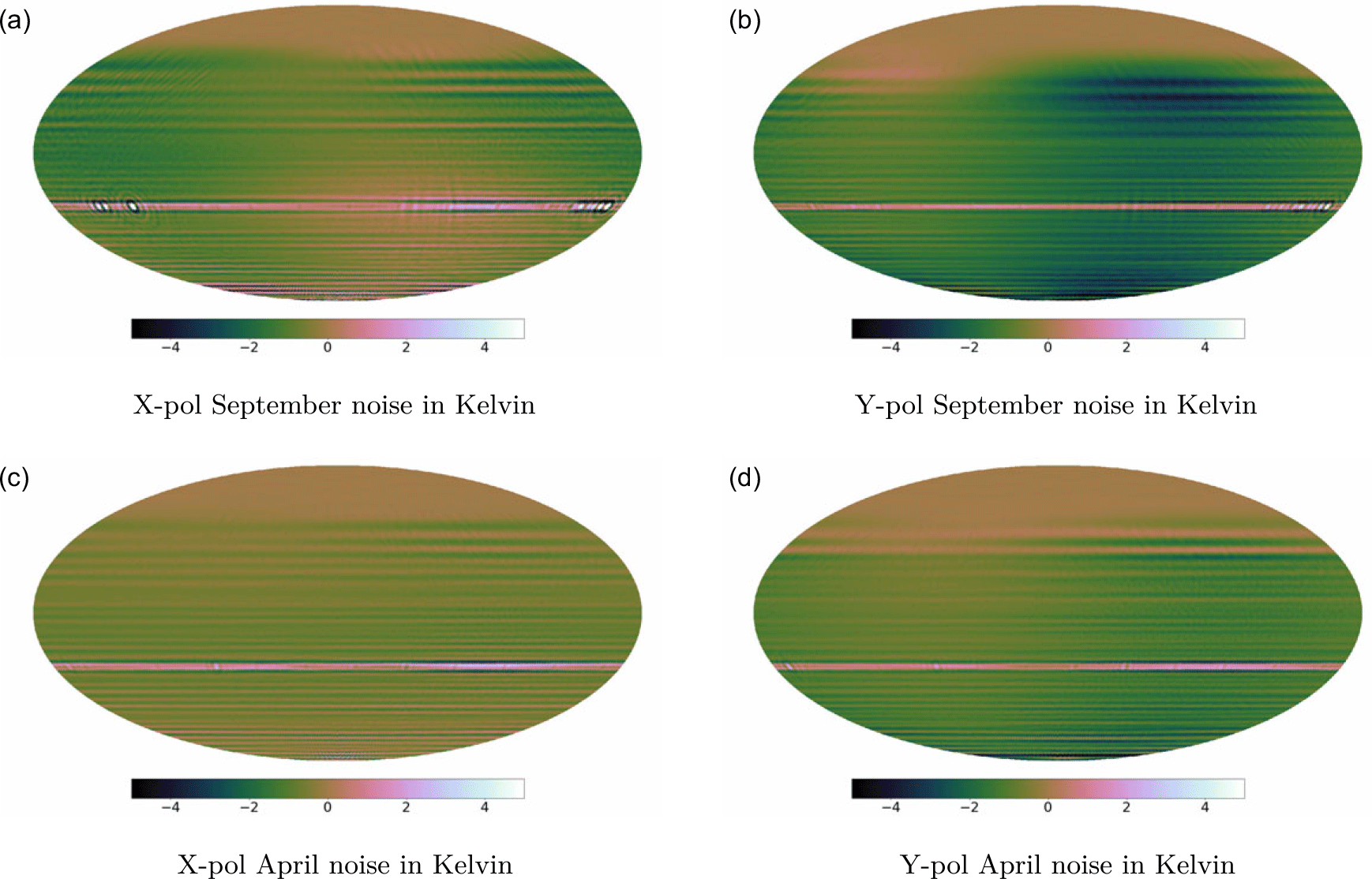
Figure 15. Equatorial projection of noise separated from measured visibilities after passing through the m-mode pipeline. A clear concentric ringing at multiple declinations is present clearly indicating a form of terrestial RFI or stationary noise. These noise-modes manifest in spherical harmonic modes $m\leq1$
.
$m\leq1$
.
To correct for these artefacts, Eastwood et al. (Reference Eastwood2018) removed all the $m\leq1$
modes and
$m\leq1$
modes and $l>100$
spherical harmonic coefficients from their sky maps. However, doing so has the risk of also throwing away actual sky information. Instead, we decomposed all noise maps and subtracted their actual contributions in
$l>100$
spherical harmonic coefficients from their sky maps. However, doing so has the risk of also throwing away actual sky information. Instead, we decomposed all noise maps and subtracted their actual contributions in $m=0$
and
$m=0$
and $m=1$
from our spherical harmonic sky coefficients in both the prior and non-prior fit September and April data; before generating the total intensity map. We do not lose actual sky information, but purely subtract what is present in modes of
$m=1$
from our spherical harmonic sky coefficients in both the prior and non-prior fit September and April data; before generating the total intensity map. We do not lose actual sky information, but purely subtract what is present in modes of $m\leq1$
in the noise maps. After generating the total intensity map we subtract the noise-subtracted intensity maps from the same combined intensity maps where we’ve omitted the noise subtraction. The residual is shown in Figure 16, it can be seen no additional artefacts have been introduced.
$m\leq1$
in the noise maps. After generating the total intensity map we subtract the noise-subtracted intensity maps from the same combined intensity maps where we’ve omitted the noise subtraction. The residual is shown in Figure 16, it can be seen no additional artefacts have been introduced.
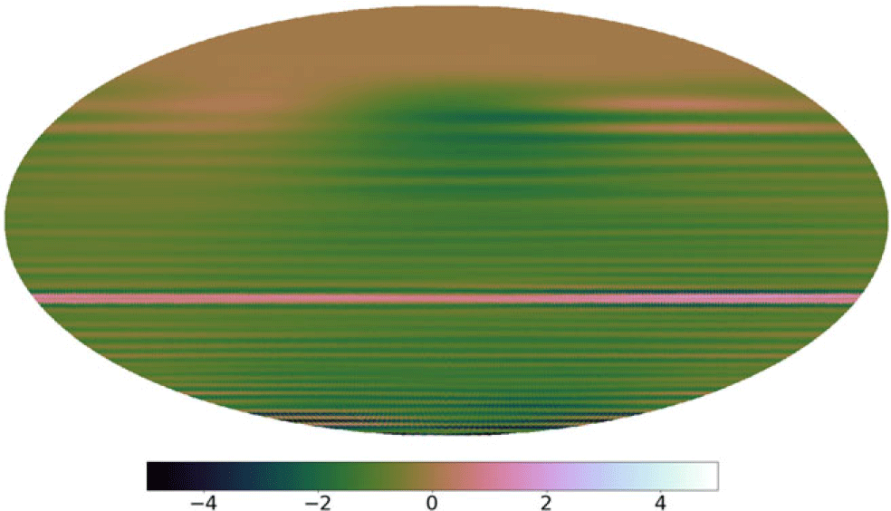
Figure 16. Map of the total systematic noise we removed from our final intensity maps in Kelvin. This map was generated by calculating the difference between a noise-corrected version of our final maps and an uncorrected version.
4.1.2. Thermal noise
We expect the maps to be confusion limited because many hours of data goes into each pixel on the sky. To verify this we have extracted the visibility noise of our two observations, using the $m>1$
modes of our imaged difference visibility data set of Subsection 4.1.1. We measured the root mean square (RMS) of the noise in a
$m>1$
modes of our imaged difference visibility data set of Subsection 4.1.1. We measured the root mean square (RMS) of the noise in a $10^{\circ}$
region independently in the September and April data; at
$10^{\circ}$
region independently in the September and April data; at $49.8^{\circ}$
RA,
$49.8^{\circ}$
RA, $-13^{\circ}$
DEC and
$-13^{\circ}$
DEC and $204.7^{\circ}$
RA,
$204.7^{\circ}$
RA, $-13^{\circ}$
DEC respectively (which is well away from the galactic plane and other strong sources). This resulted in a noise estimate of 0.024 K for September and 0.037 K for April. The magnitude of the noise measurements for X and Y were virtually identical. We compared these values to the standard deviations we extracted from the final sky map in the same regions; which are 10.06 and 14.8 K respectively.
$-13^{\circ}$
DEC respectively (which is well away from the galactic plane and other strong sources). This resulted in a noise estimate of 0.024 K for September and 0.037 K for April. The magnitude of the noise measurements for X and Y were virtually identical. We compared these values to the standard deviations we extracted from the final sky map in the same regions; which are 10.06 and 14.8 K respectively.
A total intensity noise map with $m\leq1$
subtracted is shown in Figure 17. This map is bias corrected on the X and Y polarisations for both September and April data and is then weighted averaged together, identical to as is performed on the final sky maps. The total map RMS is measured to be 0.073 K. However, a clear systematic residual, albeit small in overall scale, is present in our September noise data between and RA of 19 and 21 h. We’ve measured the RMS of this systematic to be 0.103 K. Furthermore, there is a bright streak around
$m\leq1$
subtracted is shown in Figure 17. This map is bias corrected on the X and Y polarisations for both September and April data and is then weighted averaged together, identical to as is performed on the final sky maps. The total map RMS is measured to be 0.073 K. However, a clear systematic residual, albeit small in overall scale, is present in our September noise data between and RA of 19 and 21 h. We’ve measured the RMS of this systematic to be 0.103 K. Furthermore, there is a bright streak around $-26.7^\circ$
in declination (zenith), which is likely a source of interference. The RMS of this streak is 0.24 K.
$-26.7^\circ$
in declination (zenith), which is likely a source of interference. The RMS of this streak is 0.24 K.
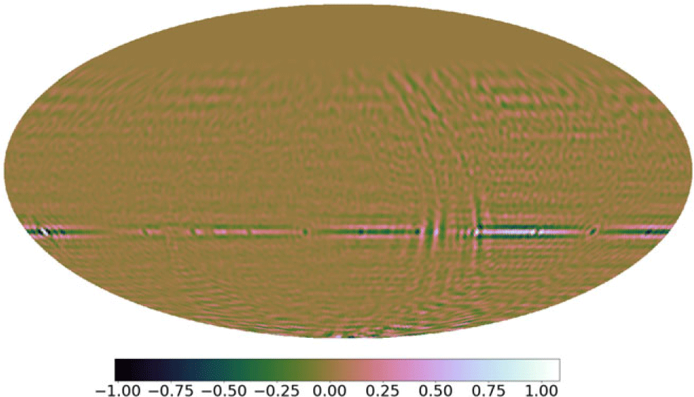
Figure 17. Noise intensity map in Kelvin, generated after removing the $m\leq1$
modes from the noise maps in Figure 15, then applying bias correction and weighted averaging as is performed on the sky maps.
$m\leq1$
modes from the noise maps in Figure 15, then applying bias correction and weighted averaging as is performed on the sky maps.
4.2. Effects of incorporating the prior
To show where the prior imposes constraints on the sky, a relative fraction difference map has been made between the unconstrained map and the map with the prior. We calculated this difference map by subtracting our non-prior map from our prior constrained map and then dividing by our non-prior map. It should be noted that in the unconstrained map a global sky component has been inserted to properly subtract the maps from each other, a sky temperature of 247 K has been selected in accordance to global sky measurements in McKinley et al. (Reference McKinley, Trott, Sokolowski, Wayth, Sutinjo, Patra, Nambissan and Ung2020). The resulting difference map is depicted in Figure 18, here it can be seen that both of our non-prior and prior fit sky maps seem to be in agreement on the galactic plane and most diffuse regions with up to 5% difference. The prior does seem to impose constraints on the diffuse emissions around the galactic plane, increasing temperatures between 15%–25% relative to the non-prior fit map. The bright area at the top is likely to be an artefact of our weighting scheme shown in Figure 11 where we down-weigh the sky towards the global sky component in the non-prior fit map, which has added diffuse galactic plane emissions in the prior fit map; resulting in a temperature discrepancy.
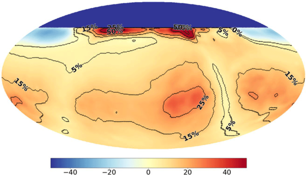
Figure 18. Relative difference between our prior-fit and unconstrained map (in %, equatorial projection). Large scale diffuse emission matches between maps within 5%, the galactic plane is in agreement too. Primarily the diffuse emission around the galactic plane is upscaled by the prior with 15%–30% more contribution.
4.3. Bias correction
The process of regularisation inevitably introduces bias when minimising the overall cost function. To calculate the bias introduced, we simulated visibilities with a known input map and compared the resulting output which we constrained with a desourced version of the input. For the known map, we used the Haslam map by Remazeilles et al. (Reference Remazeilles, Dickinson, Banday, Bigot-Sazy and Ghosh2015), which we reprojected to equatorial coordinates and rescaled to our HEALPix pixel grid; similar to how we created the prior for the EDA2 map, but excluding the Gaussian smoothing. We subsequently generated two sets of images of the sky, separated by 1 min of LST, whilst embedding the EDA2 X and Y polarisation beam patterns; this to cover a full sidereal day. Using these beam-weighted sky models, we employed Miriad (Sault, Teuben, & Wright Reference Sault, Teuben, Wright, Shaw, Payne and Hayes1995) using the EDA2’s layout to generate 24 h worth of visibilities which were provided to our m-mode pipeline as input to image the sky. Given the input model map is at the same frequency and angular scales as the EDA2 159 MHz sky map, we do not expect the Tikhonov factor to deviate and kept $\varepsilon=0.1$
for the imaging process.
$\varepsilon=0.1$
for the imaging process.
The resulting output X-polarisation and Y-polarisation maps we used to calculate the percentage fractional difference relative to the known input map. This sets all correct values on the sky to zero and any bias shows up as a percentage offset. These bias maps are shown in Figure 19. From Figure 19 it is evident a dipole-like structure is present overestimating the one side of the image and underestimating the other. This can be clearly attributed to improper constraints on the $l=1$
spherical harmonic coefficients; smaller angular scales on the sky match the input on the sky and therefore do not appear in the bias. These offsets range from +10% at its peak to –10% at its lowest for the X-polarisation, similar for the Y-polarisation with a small negative region of –20% offset.
$l=1$
spherical harmonic coefficients; smaller angular scales on the sky match the input on the sky and therefore do not appear in the bias. These offsets range from +10% at its peak to –10% at its lowest for the X-polarisation, similar for the Y-polarisation with a small negative region of –20% offset.
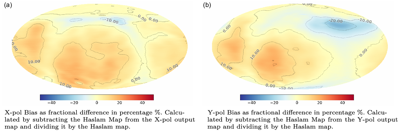
Figure 19. Average bias between our known Haslam input map and our prior fit output maps (in %, equatorial projection). Left: X-polarisation bias, Right: Y-polarisation bias. A clear dipole effect is presents with 10% deviation.
Since we divided out the true sky, that is, our known input, we can correct for the bias as the bias map only represents relative over- and under-estimations. We apply these correction through employing the bias maps as weighting schemes on our noise-corrected X-polarisation and Y-polarisation maps before generating our weighted intensity maps. The weighting scheme is defined by
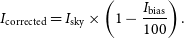 \begin{align} I_{\textrm{corrected}} &= I_{\textrm{sky}} \times \left(1-\frac{I_{\textrm{bias}}}{100}\right).\end{align}
This allows us to down weigh the overestimated regions on the sky and upscale the underestimated ones.
5. Analysis
In this section we compare how the non-prior map and prior constrained EDA2 159 MHz map compares to existing sky models. We compare the maps to the frequently used global sky model (GSM) both the reprocessed version from 2016 (Zheng et al. Reference Zheng2017) and the 2008 version (De Oliveira-Costa et al. Reference De Oliveira-Costa2008), the reprocessed desourced Haslam map (Remazeilles et al. Reference Remazeilles, Dickinson, Banday, Bigot-Sazy and Ghosh2015), and the Long Wavelength Array (LWA)1 lowfrequency sky survey (LFSS) (Dowell et al. Reference Dowell2017). For all these sky models we use pyGDSM (Price Reference Price2016) to rescale the maps to 159 MHz to which we then applied NSIDE rescaling and smoothing to the EDA2 angular resolution; prior to comparing the data. We compare the EDA2 159 MHz maps to the sky models by calculating the relative fractional difference between the two maps. This is defined by
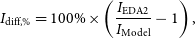 \begin{align} I_{\textrm{diff,%}} &= 100\% \times \left(\frac{I_{\textrm{EDA2}}}{I_{\textrm{Model}}}-1\right),\end{align}
Positive values indicate the EDA2 maps are brighter, negative values indicate the sky model maps are brighter.
5.1. 2008 global sky model
The difference maps between our EDA2 maps and the 2008 GSM (De Oliveira-Costa et al. Reference De Oliveira-Costa2008) are shown in Figures 20 and 21, we compare the non-prior vs the sky model and the prior vs the sky model respectively. Since the pyGDSM rescaled 2008 GSM map is desourced we mask off any bright sources in our EDA2 map, as well as the region in the sky we do not observe in our map that has not been constrained by a prior. Figure 20 shows that generally we are 12% higher in temperature compared to the GSM off the Galactic Centre. Near the Galactic Centre, we notice we are on average 18% lower in diffuse emission. Dowell et al. (Reference Dowell2017) noticed a similar effect in their comparison to the GSM. The difference is likely a cause of improper constraints on the free-free emission in the higher frequency maps that primarily make up the sky model. There is also a clear striping artefact present in the fractional difference maps between an RA of approximately 5 and 12 h, which is an imaging artefact in the GSM, likely caused when combining the individual maps to make up the model.
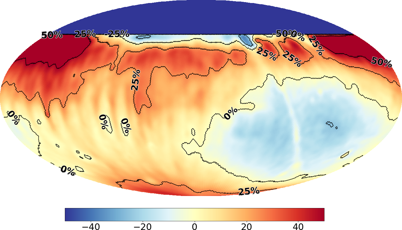
Figure 20. Comparison between our non-prior EDA2 159 MHz sky map and the 2008 GSM of De Oliveira-Costa et al. (Reference De Oliveira-Costa2008) rescaled to 159 MHz; in percentage and equatorial coordinates. The comparison is made by dividing our sky map by the GSM at 159 MHz and is then offset by 1 to put zero difference on regions that agree. Contours have been overlaid to show a difference in scales across the map. Our map shows 18% less contribution in the diffuse emission around the Galactic Centre, but is generally approximately 12% brighter.
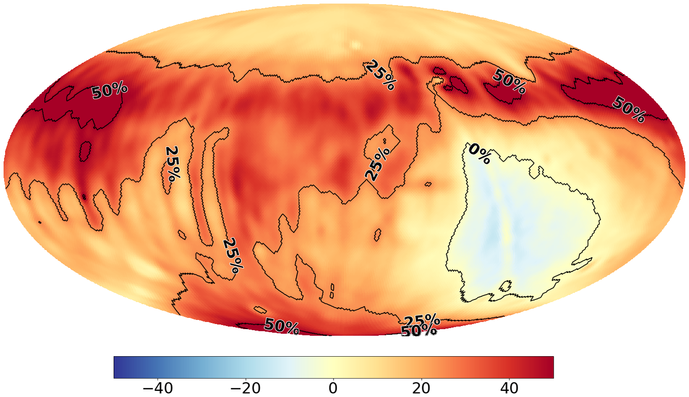
Figure 21. Comparison between our Haslam prior constrained EDA2 159 MHz sky map and the 2008 GSM of De Oliveira-Costa et al. (Reference De Oliveira-Costa2008) rescaled to 159 MHz; in percentage and equatorial coordinates. The comparison is done using the same method as in to Figure 20. With the prior-fit map, the diffuse emission around the galactic plane matches better; ranging from 0% to 10% difference. However, in general, our prior-fit sky map is approximately 25% brighter.
Comparing our Haslam prior constrained EDA2 sky map to the 2008 GSM at 159 MHz shows that the prior constrains the diffuse emission around the Galactic Centre and more closely matches the diffuse emissions from the GSM with between 0% to 10% difference. However, anywhere else our prior constraint increased our relative brightness compared to the GSM to 25% difference on average. It should be noted that for both the non-prior and prior constrained EDA2 sky maps we have 25% more contribution around the southern celestial pole.
5.2. 2016 global sky model
We also generated the fractional differences between the EDA2 non-prior and prior constrained map and the 159 MHz 2016 GSM of Zheng et al. (Reference Zheng2017). The difference maps are shown in Figures 22 and 23. Figure 22 shows that in the no-prior map we are 17% brighter on average, with regions of 25% difference under the galactic plane. The reprocessed GSM, however, is more in agreement with our maps in the diffuse emission around the Galactic Centre, with an average of 12% difference. Imaging artefacts from the 2008 GSM, although less prevalent, are still present.
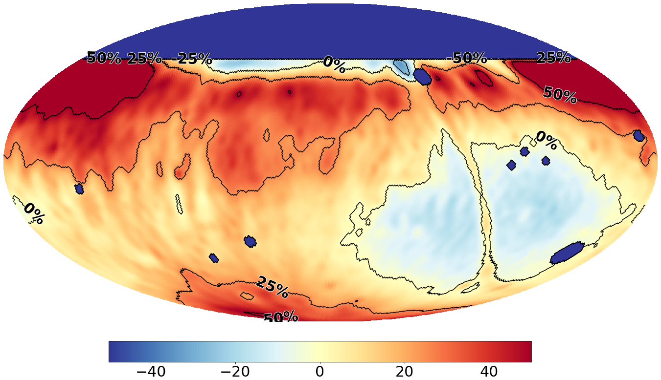
Figure 22. Comparison between non-prior EDA2 159 MHz sky map and the 2016 GSM of Zheng et al. (Reference Zheng2017) rescaled to 159 MHz; in percentage and equatorial coordinates. In general, our map is on average 17%–25% brighter, but our maps closer resembles the diffuse emission around the Galactic Centre, with an average of 12% difference, compared to the 2008 GSM
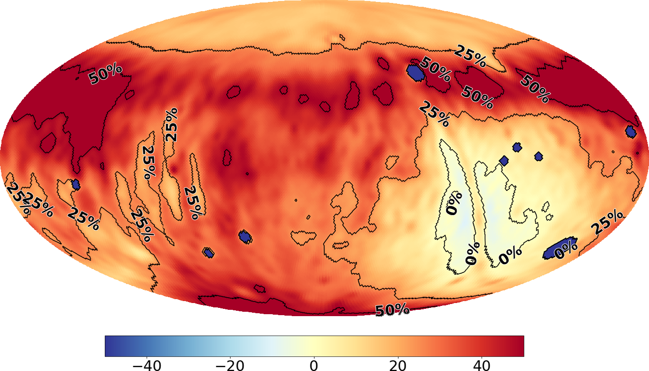
Figure 23. Comparison between our Haslam prior constrained EDA2 159 MHz sky map and the 2016 GSM of Zheng et al. (Reference Zheng2017) rescaled to 159 MHz; in percentage and equatorial coordinates. We have a consistent offset of 25%, however are more in agreement with the galactic plane with 3% difference on average.
The prior constrained EDA2 sky map closer matches the diffuse emission around the Galactic Centre, up to a few percent difference. However, the constrained map is on average 25% brighter than the 2016 GSM. The south celestial poles for both EDA2 sky maps show up to 25%–50% difference compared to the 2016 GSM. Comparing this to GSM comparisons with the LWA sky maps by Dowell et al. (Reference Dowell2017), we see differences of similar magnitudes in the diffuse emission regions.
5.3. 2014 Reprocessed Haslam map
Since we constrain our map with the desourced reprocessed 2014 Haslam map by Remazeilles et al. (Reference Remazeilles, Dickinson, Banday, Bigot-Sazy and Ghosh2015), we compare our EDA2 sky maps to the Haslam map to make sure we do not force our map to be identical to Haslam. In Figure 24 we compare our non-prior EDA2 map with the Haslam map. We are 3%–6% less bright on average and 6% brighter at declinations higher than $30^{\circ}$
. However, the Haslam map is up to 25% brighter in the diffuse emission around the Galactic Centre.
$30^{\circ}$
. However, the Haslam map is up to 25% brighter in the diffuse emission around the Galactic Centre.
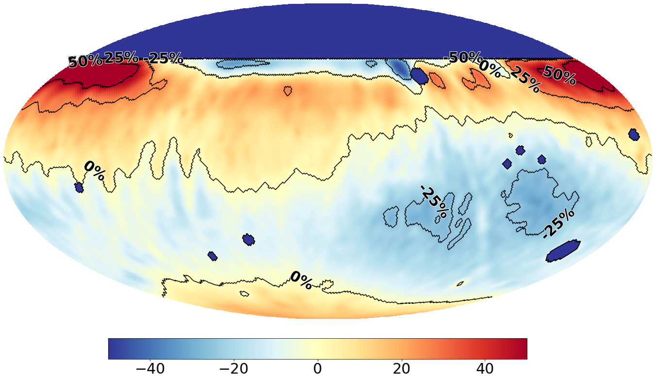
Figure 24. Comparison between non-prior EDA2 159 MHz sky map and the desourced 2014 reprocessed Haslam map (Remazeilles et al. Reference Remazeilles, Dickinson, Banday, Bigot-Sazy and Ghosh2015) rescaled to 159 MHz; in percentage and equatorial coordinates. In general we are better in agreement compared to both GSMs and are on average –3%–6% different. However, the Haslam also shows excess (25%) in galactic diffuse emission near the Galactic Centre compared to the EDA2
For our prior constrained map (Figure 25) we are in overall better agreement. This is expected since we use the Haslam map as a prior to constrain our coefficients. However, there are still differences. In most regions above the southern celestial pole and below $30^{\circ}$
declination we are on average 3%–6% brighter than Haslam. The overall contribution of EDA2 increases up to 12%–25% above
$30^{\circ}$
declination we are on average 3%–6% brighter than Haslam. The overall contribution of EDA2 increases up to 12%–25% above $30^{\circ}$
declination. We also match the galactic plane closely with 3% difference. The diffuse emissions around the Galactic Centre more closely matches the Haslam map, where we are 7% less bright on average. The Southern celestial pole still shows similar contribution of 10%–25% brighter compared to Haslam.
$30^{\circ}$
declination. We also match the galactic plane closely with 3% difference. The diffuse emissions around the Galactic Centre more closely matches the Haslam map, where we are 7% less bright on average. The Southern celestial pole still shows similar contribution of 10%–25% brighter compared to Haslam.
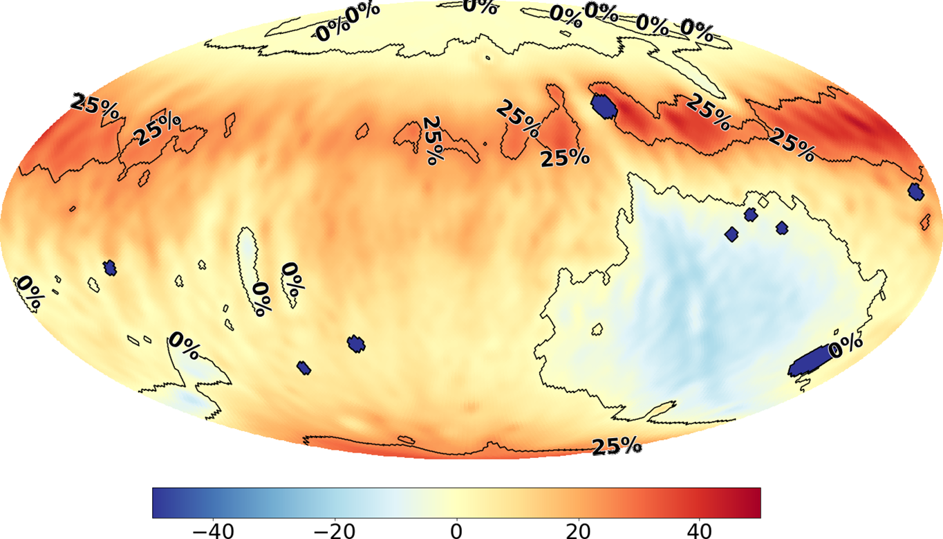
Figure 25. Comparison between our Haslam prior constrained EDA2 159 MHz sky map and the desourced 2014 reprocessed Haslam map (Remazeilles et al. Reference Remazeilles, Dickinson, Banday, Bigot-Sazy and Ghosh2015) rescaled to 159 MHz; in percentage and equatorial coordinates. We have better overall agreement with 3%–6% difference, which is expected as we use the same map to fit the prior. We also closely match the galactic plane with an average of 3% in excess. However, we see excess emissions in our map up to 12%–25% at declinations $\ge30^{\circ}$
.
$\ge30^{\circ}$
.
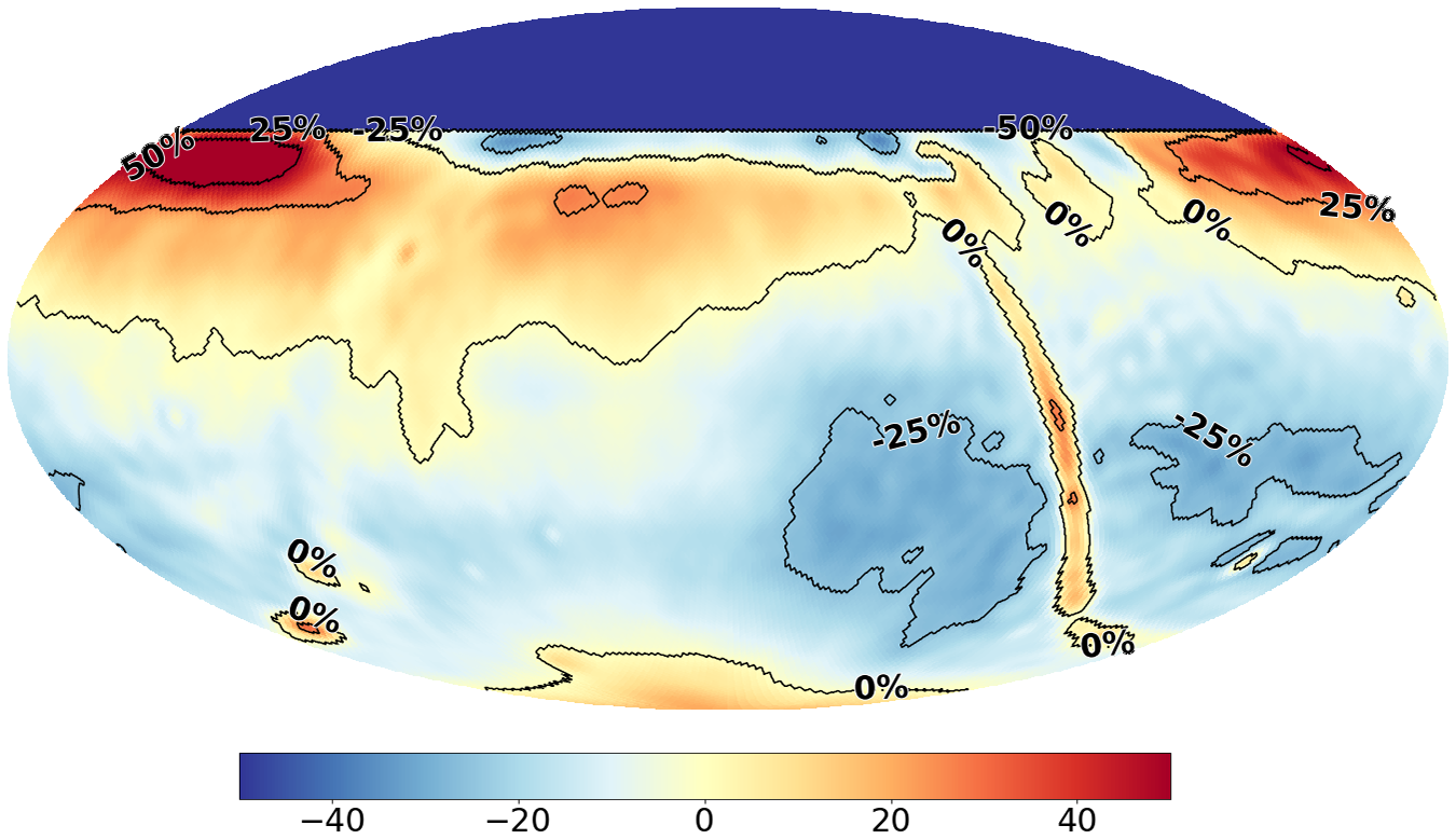
Figure 26. Comparison between our non-prior EDA2 159 MHz sky map and the LFSS (Dowell et al. Reference Dowell2017) rescaled to 159 MHz; in percentage and equatorial coordinates. We are lesser in agreement around the galactic plane, where we are 25% less in contribution. This is likely caused do to the fact the LFSS is more diffuse compared to the EDA2 map. Furthermore, the LFSS has on average 25% more contribution in the diffuse emissions around the galactic plane compared to the non-prior fit map. However, in all other regions on the sky we seem in overall better agreement than compared to any other sky model where we have between 0%–10% difference on average.
Similar to the 2008 and 2016 GSM we see similar striping between PicA and VirA in the Haslam map; albeit more subtle.
5.4. LWA1 low-frequency sky survey
To see how the EDA2 sky maps compares to sky maps made at lower frequencies, we compare the EDA2 maps to the LWA1 LFSS by Dowell et al. (Reference Dowell2017). For our non-prior map comparison (Figure 26) we are in good agreement with the LFSS with differences between 0% to 10%; except for near the galactic plane. In the galactic plane we have 25% more contribution compared to the LFSS, we expect this due to H $_{\textrm{II}}$
regions in the galactic plane. We do not see any of the imaging artefacts we identified in the Haslam and GSM maps.
$_{\textrm{II}}$
regions in the galactic plane. We do not see any of the imaging artefacts we identified in the Haslam and GSM maps.
The prior constrained EDA2 sky map is in much better agreement with the LFSS in general. In Figure 27 we closely follow the LFSS up to declinations of $45^{\circ}$
and have on average –4%–4% difference. we have on average 7% less contribution in diffuse emission around the Galactic Centre, however still see up to 25% in excess on the galactic plane. The 50% difference at Vela is likely a product of SI between the Haslam prior and the LFSS; since we do not see it in our map that is not prior constrained. It should be noted that compared to the LFSS the EDA2 sky maps also show more contributions at the south celestial pole, which are again 10%–25% brighter.
$45^{\circ}$
and have on average –4%–4% difference. we have on average 7% less contribution in diffuse emission around the Galactic Centre, however still see up to 25% in excess on the galactic plane. The 50% difference at Vela is likely a product of SI between the Haslam prior and the LFSS; since we do not see it in our map that is not prior constrained. It should be noted that compared to the LFSS the EDA2 sky maps also show more contributions at the south celestial pole, which are again 10%–25% brighter.
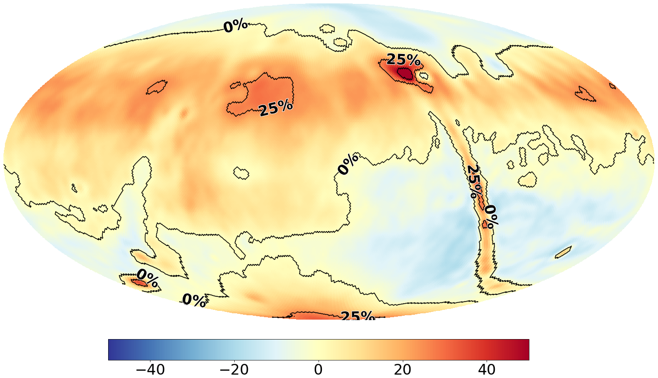
Figure 27. Comparison between the prior fit EDA2 159 MHz sky map and the LFSS (Dowell et al. Reference Dowell2017) rescaled to 159 MHz; in percentage and equatorial coordinates. We have much better agreement compared to all other sky models, bar the galactic plane. In general we seem to closely match the diffuse emissions up to $40^{\circ}$
in declination, where we have –4%–4% difference.
$40^{\circ}$
in declination, where we have –4%–4% difference.
5.5. A comment on systematics
To determine whether the relative fractional differences are in the same order of magnitude compared to the differences between the sky models we compare to, we calculated the mean temperatures in a 10 degree radius in the diffuse region at 1 h in RA and $-26.7^{\circ}$
in DEC (zenith). These temperatures range from 202 K for the 2016 GSM (Zheng et al. Reference Zheng2017) to 247 K for the LFSS (Dowell et al. Reference Dowell2017), resulting in an approximate 18% fractional difference. For our maps, calculate the mean temperatures in the same region. In this region, our no-prior map has a mean temperature of 215 K and our prior constrained map has a mean temperature of 253 K. These values fall into the same approximate range of temperatures found when comparing the individual sky models, explaining the difference in fractional difference we see between our maps and the sky models.
$-26.7^{\circ}$
in DEC (zenith). These temperatures range from 202 K for the 2016 GSM (Zheng et al. Reference Zheng2017) to 247 K for the LFSS (Dowell et al. Reference Dowell2017), resulting in an approximate 18% fractional difference. For our maps, calculate the mean temperatures in the same region. In this region, our no-prior map has a mean temperature of 215 K and our prior constrained map has a mean temperature of 253 K. These values fall into the same approximate range of temperatures found when comparing the individual sky models, explaining the difference in fractional difference we see between our maps and the sky models.
When comparing EDA2 with all aforementioned sky models, we note that the EDA2 non-prior and prior-constrained sky maps both have a consistent relative offset in temperature most prominent at declinations between $50^{\circ}$
and
$50^{\circ}$
and $60^{\circ}$
; which is an apparent systematic bias in our maps. We reiterate that the sky above
$60^{\circ}$
; which is an apparent systematic bias in our maps. We reiterate that the sky above $40^{\circ}$
in DEC is poorly measured by our system, as shown in Figures 4 and 5 the y-polarisation dipole gain falls more quickly with increasing declination; it reaches 10% at
$40^{\circ}$
in DEC is poorly measured by our system, as shown in Figures 4 and 5 the y-polarisation dipole gain falls more quickly with increasing declination; it reaches 10% at $+32^{\circ}$
in DEC and 5% at
$+32^{\circ}$
in DEC and 5% at $+40^{\circ}$
. We do not expect this to be due to other causes as we did not identify this systematic in our bias maps, as is evident in Section 4.3.
$+40^{\circ}$
. We do not expect this to be due to other causes as we did not identify this systematic in our bias maps, as is evident in Section 4.3.
We also note that the morphology of the fractional differences in all of the comparison maps, for example, where our map is less bright around the galactic plane, is similar. This morphology does not match the morphology of the biases seen in Figure 19. We therefore interpret these to be genuine differences in the local SIs of these maps, rather than being due to a systematic effect of the m-mode imaging.
5.6. Spectral index map
Figure 28 shows the spectral index derived from our EDA2 map when rescaled to the 408 MHz Haslam map which has been reprojected to equatorial coordinates and smoothed to the same angular resolution of 3.1 degrees. The Haslam map has been extracted from pyGDSM (Price Reference Price2016) which is assumed to have a flat SI of 2.6 across the sky. We see the largest difference in our maps at the galactic plane, where we measure an SI of 2.4–2.45 more in accordance to the SIs derived by Dowell et al. (Reference Dowell2017). The diffuse emission around the Galactic Centre we calculated to have an SI of 2.5 on average. The remaining diffuse emission ranges from 2.6–2.7 in SI. SIs calculated above $40^{\circ}$
in declination we do not deem trustworthy due to the systematic bias we discussed in Subsection 5.5. The reason we see the major difference around the galactic plane is likely due to the fact a single-power law assumption start breaking down when having significant discrepancy in frequency, as
$40^{\circ}$
in declination we do not deem trustworthy due to the systematic bias we discussed in Subsection 5.5. The reason we see the major difference around the galactic plane is likely due to the fact a single-power law assumption start breaking down when having significant discrepancy in frequency, as $\textrm{H}_{\textrm{II}}$
regions become more prevalent due to thermal absorption (Dowell et al. Reference Dowell2017; Kassim Reference Kassim1989). To properly define SIs for the EDA2 observed sky, more comparisons and observations across multiple frequencies have to be made. However, this is out of scope for this paper and we will address this in future work.
$\textrm{H}_{\textrm{II}}$
regions become more prevalent due to thermal absorption (Dowell et al. Reference Dowell2017; Kassim Reference Kassim1989). To properly define SIs for the EDA2 observed sky, more comparisons and observations across multiple frequencies have to be made. However, this is out of scope for this paper and we will address this in future work.
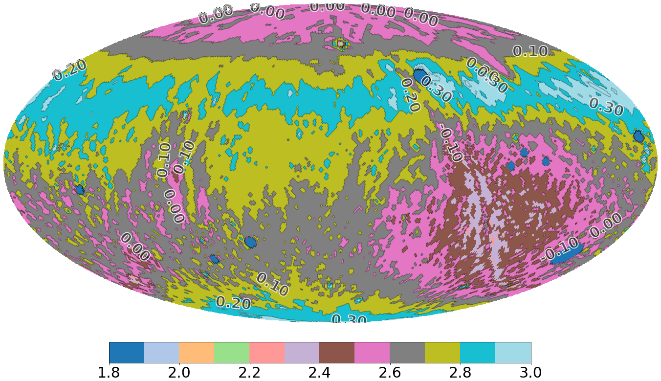
Figure 28. Spectral index map calculated between our prior-constrained EDA2 map and the desourced Haslam map of Remazeilles et al. (Reference Remazeilles, Dickinson, Banday, Bigot-Sazy and Ghosh2015). We overlaid the absolute difference in SI between our map and the Haslam map as labeled contours. Bright sources have been masked off.
6. Conclusions
We present two EDA2 159 MHz all-sky maps generated using the novel imaging method known as the m-mode formalism. We have shown how prior-fitting the Tikhonov regularisation, first suggested by Eastwood et al. (Reference Eastwood2018), puts constraints on the diffuse emissions on the sky for modes we are not, or less, sensitive to. Furthermore, we have shown how we can remove systematic bias from our sky maps implemented as a weighting scheme, and how we can correct for terrestrial noise by down weighting those specific modes in coefficient space; without compromising actual information on the sky. To generate these maps, two observations have been performed, separated by a 7 month interval, in order to remove the sun. For both observations 24 h of data have been used. The maps are created with a maximum angular resolution of $3.1^\circ$
, within the time-frame of a single day. These maps have
$3.1^\circ$
, within the time-frame of a single day. These maps have $<0.5$
K measured thermal noise and are super sampled on a 0.91 degree pixel grid.
$<0.5$
K measured thermal noise and are super sampled on a 0.91 degree pixel grid.
Between declination range of $-70^{\circ}$
and
$-70^{\circ}$
and $+40^{\circ}$
our maps on average have approximately 10% relative difference compared to the reprocessed Haslam map (Remazeilles et al. Reference Remazeilles, Dickinson, Banday, Bigot-Sazy and Ghosh2015) and the LFSS (Dowell et al. Reference Dowell2017); and 25% difference of the GSMs (De Oliveira-Costa et al. Reference De Oliveira-Costa2008; Zheng et al. Reference Zheng2017). At higher declinations above
$+40^{\circ}$
our maps on average have approximately 10% relative difference compared to the reprocessed Haslam map (Remazeilles et al. Reference Remazeilles, Dickinson, Banday, Bigot-Sazy and Ghosh2015) and the LFSS (Dowell et al. Reference Dowell2017); and 25% difference of the GSMs (De Oliveira-Costa et al. Reference De Oliveira-Costa2008; Zheng et al. Reference Zheng2017). At higher declinations above $40^{\circ}$
our maps are not well measured. We also show a consistent 10%–25% higher temperature around the southern celestial pole.
$40^{\circ}$
our maps are not well measured. We also show a consistent 10%–25% higher temperature around the southern celestial pole.
We also generated an all-sky thermal noise intensity map with an average RMS of 0.073 K across the observed sky. In this map, there is some systematic/interference between RA of 19 and 21 h and at $-26.7^{\circ}$
in declination (zenith), with a maximum RMS of 0.24 K. However, compared to the temperature variations on quiet regions on the sky (approximately 10–14 K), the thermal noise (including the systematics) is roughly 2 orders of magnitude lower. Because our maps are confusion limited they would form one part of a complete foreground model for EoR sciences, but can be used as-is for single-antenna total power measurements. Byrne et al. (Reference Byrne, Morales, Hazelton, Sullivan, Barry, Lynch, Line and Jacobs2021) have shown that the angular scale at which power of diffuse emissions and point sources are equal is in the order of several degrees, therefore diffuse sky maps such as these will be required for complete calibration models in the future.
$-26.7^{\circ}$
in declination (zenith), with a maximum RMS of 0.24 K. However, compared to the temperature variations on quiet regions on the sky (approximately 10–14 K), the thermal noise (including the systematics) is roughly 2 orders of magnitude lower. Because our maps are confusion limited they would form one part of a complete foreground model for EoR sciences, but can be used as-is for single-antenna total power measurements. Byrne et al. (Reference Byrne, Morales, Hazelton, Sullivan, Barry, Lynch, Line and Jacobs2021) have shown that the angular scale at which power of diffuse emissions and point sources are equal is in the order of several degrees, therefore diffuse sky maps such as these will be required for complete calibration models in the future.
Furthermore, we introduced a variation to the image deconvolution algorithm of Eastwood et al. (Reference Eastwood2018). This algorithm operates in image space by taking advantage of the fact the PSF is shift-invariant in right ascension.
Finally, we introduced a formalism to inspect the interferometer’s sensitivity in spherical harmonic coefficient space, analogous to the $u, v$
-plane coverage in traditional interferometry; showing the m-mode formalism allows for sensitivity to diffuse emission much larger in angular scales than traditional snapshot imaging provides. We also show how the spherical harmonic beam coverage can aid in better constraining a prior.
$u, v$
-plane coverage in traditional interferometry; showing the m-mode formalism allows for sensitivity to diffuse emission much larger in angular scales than traditional snapshot imaging provides. We also show how the spherical harmonic beam coverage can aid in better constraining a prior.
Acknowledgements
We thank Daniel Ung for aiding in generating and providing the FEKO-generated EDA2 beam models. Additionally, we would like to thank Marcin Sokolowski and Ravi Subrahmanyan for their assistance and feedback on the EDA2 gain calibration methods. Furthermore, we thank Jaiden Cook for providing assistance and insights on Gaussian fitting algorithms. We would also like to thank the anonymous reviewer for their valuable comments, resulting in an overall improvement of this manuscript. This research was supported by the Australian Research Council Centre of Excellence for All Sky Astrophysics in Three Dimensions (ASTRO3D), through project number CE170100013. This scientific work makes use of the Murchison Radio-astronomy Observatory (MRO), operated by CSIRO. We acknowledge the Wajarri Yamatji People as the traditional owners of the observatory site. We acknowledge the Pawsey Supercomputing Centre which is supported by the Western Australian and Australian Governments. We acknowledge the use of the Legacy Archive for Microwave Background Data Analysis (LAMBDA), part of the High Energy Astrophysics Science Archive Center (HEASARC). HEASARC/LAMBDA is a service of the Astrophysics Science Division at the NASA Goddard Space Flight Center. We acknowledge the work and the support of the developers of the following Python packages: pyGDSM (Price Reference Price2016), Numpy (Harris et al. Reference Harris2020), Astropy (Astropy Collaboration et al. 2013, 2018), Healpy (Zonca et al. Reference Zonca, Singer, Lenz, Reinecke, Rosset, Hivon and Gorski2019), Scipy (Virtanen et al. Reference Virtanen2020), and Matplotlib (Hunter Reference Hunter2007). We acknowledge the work and support of the developers of the HEALPix software (Gorski et al. Reference Gorski, Hivon, Banday, Wandelt, Hansen, Reinecke and Bartelmann2005) and Miriad software (Sault et al. Reference Sault, Teuben, Wright, Shaw, Payne and Hayes1995).
A Examples of beam-coefficient space
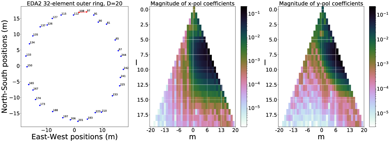
Figure A.1. Example of spherical harmonic beam coefficients for a short East-West baseline (contribution is low on spatial coefficients l and is primarily m dependant).
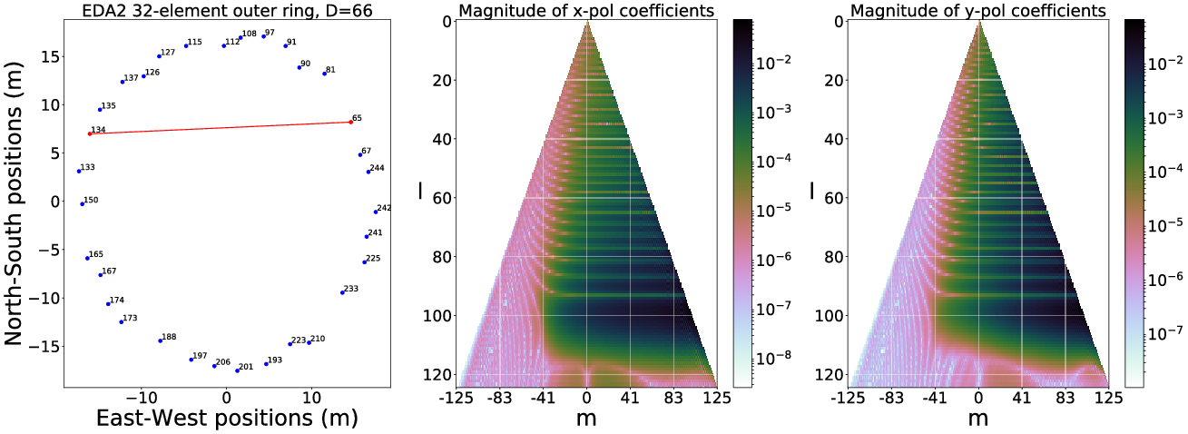
Figure A.2. Example of spherical harmonic beam coefficients for a long East-West baseline (contribution is high on spatial coefficients l and is primarily m dependant).
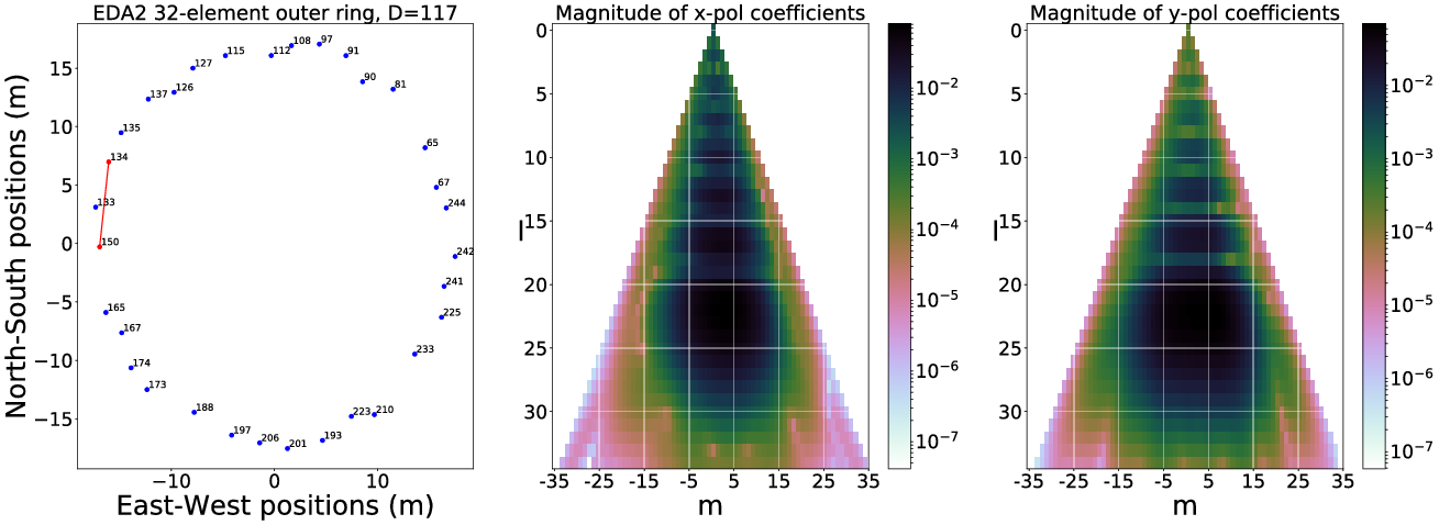
Figure A.3. Example of spherical harmonic beam coefficients for a North-South baseline (contribution is symmetric around $m=0$
).
$m=0$
).
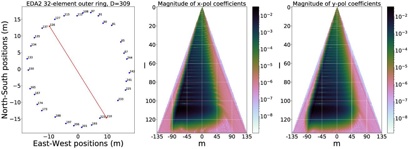
Figure A.4. Example of spherical harmonic beam coefficients for a diagonal baseline pointing North-West (contribution moves to the negative m-modes).
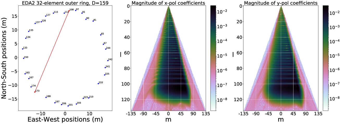
Figure A.5. Example of spherical harmonic beam coefficients for a diagonal baseline pointing North-East (contribution moves to the positive m-modes).
B Sky maps in HEALPix representation
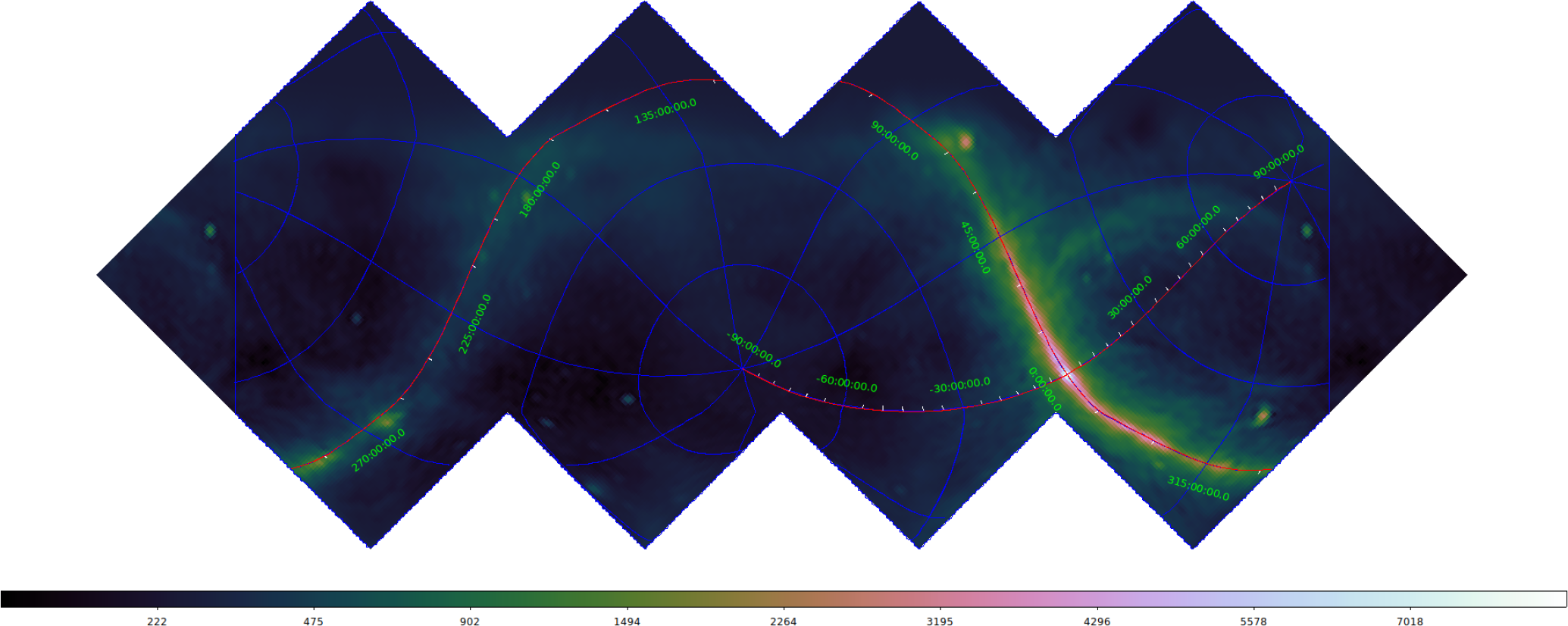
Figure B.1. 159 MHz diffuse EDA2 map (equatorial view, HEALPix RING ordering scheme), log-scale. Generated without the use of a prior model, the global sky component is reinserted.
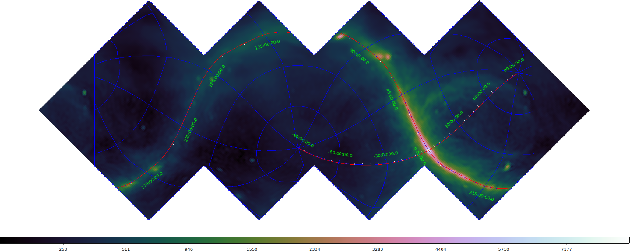
Figure B.2. 159 MHz diffuse EDA2 map (equatorial view, HEALPix RING ordering scheme), log-scale. Generated with the use of the reprocessed desourced Haslam map as a prior model to constrain the largest scales. Since we cannot observe at declinations $>60^{\circ}$
, the northern hemisphere is equivalent to the diffuse Haslam map depicted in Figure 7.
$>60^{\circ}$
, the northern hemisphere is equivalent to the diffuse Haslam map depicted in Figure 7.


 Open access