


1 INTRODUCTION
The orbital evolution of globular clusters (GCs) in the Galaxy, combined with kinematics and stellar population analyses, can provide important information to decipher the history of our Galaxy. The Galactic bulge contains a significant fraction of the GC population (~25% of GCs) in the Galaxy (Bica, Ortolani, & Barbuy Reference Bica, Ortolani and Barbuy2016). This fraction may increase significantly in coming years with analyses of recent 84 VVV bulge GC candidates (Minniti et al. Reference Minniti2017a, Minniti, Alonso-Garca, & Pullen Reference Minniti, Alonso-Garca and Pullen2017b). In spite of this, very few attempts have been made so far to study the orbits of bulge clusters, previously prevented mainly due to high reddening, crowding, and distance effects.
Two main pieces of information are needed in order to determine the Galactic orbit of a GC: the Galactic position and velocity components of the cluster and a mass model of the Galaxy. The position and velocity components form a six-dimensional vector, called initial state vector, representing the initial conditions required to solve the equations of motion (EoM) associated with the gravitational potential generated by the host galaxy. In this approach, the cluster is treated as a test particle. This is the typical approximation to study GCs orbits (Aguilar, Hut, & Ostriker Reference Aguilar, Hut and Ostriker1988; Gnedin & Ostriker Reference Gnedin and Ostriker1997; Gnedin, Lee, & Ostriker Reference Gnedin, Lee and Ostriker1999; Dinescu et al. Reference Dinescu, Majewski, Girard and Cudworth2001; Casetti-Disnescu et al. Reference Casetti-Dinescu2007, Reference Casetti-Dinescu2013; Pichardo, Martos, & Moreno Reference Pichardo, Martos and Moreno2004; Allen, Moreno, & Pichardo Reference Allen, Moreno and Pichardo2006, Reference Allen, Moreno and Pichardo2008; Ortolani et al. Reference Ortolani, Barbuy, Momany, Saviane, Bica, Jilkova, Salerno and Jungwiert2011; Moreno, Pichardo, & Velázquez Reference Moreno, Pichardo and Velázquez2014). Even in works where the destruction rates and tidal stripping are studied in depth (e.g. Moreno et al. Reference Moreno, Pichardo and Velázquez2014), the calculation of the orbits is carried out under the assumption that the cluster acts as a test particle, and it is over such invariant orbit that individual clusters (including N-body model clusters) are calculated (Jílková et al. Reference Jílková, Carraro, Jungwiert and Minchev2012; Martinez-Medina et al. Reference Martinez-Medina, Gieles, Pichardo and Peimbert2018). In general, for massive clusters (i.e. the ones we see today), the effect of mass loss on the orbit is negligible. Even in clusters that go through substantial mass loss, where part of the mass loss is expected to be due to evaporation across all the surface of the cluster and part to tidal effects (bipolar), neither is expected to affect the centre of mass of the remaining cluster, and consequently it will not affect the orbit.
In our previous paper (Rossi et al. Reference Rossi, Ortolani, Barbuy, Bica and Bonfanti2015, hereafter Paper I), we presented the relative proper motions to the bulge field stars of 10 GCs located in the Galactic bulge, namely Terzan 1, Terzan 2, Terzan 4, Terzan 9, NGC 6522, NGC 6558, NGC 6540, Palomar 6, AL 3, and ESO 456–SC38. The clusters AL3 and ESO 456–SC38 are not analysed in the present work because they have no radial velocity determinations in the literature. By combining information on the proper motion with position components and radial velocities, we derived the initial state vector of eight of the bulge clusters in our sample. For comparison purposes, we also included in the analysis the inner halo cluster NGC 6652, for which the initial state vector has been computed from proper motion data by Sohn et al. (Reference Sohn, van der Marel, Carlin, Majewski, Kallivayalil, Law, Anderson and Siegel2015).
The main goal of this follow-up paper is to construct the orbit of the bulge GCs with the purpose of checking whether they are trapped by the Galactic bar or not, and at the same time, we seek for correlations between the distribution of clusters and of their kinematic properties with metallicity that could be interpreted as due to the dynamics produced by the Galactic bar.
The present work is structured as follows. In Section 2, we present the data available for the sample GCs, that were employed in the calculations. In Section 3, the adopted mass models of the Milky Way and the process followed to integrate the orbits of the clusters and their orbital parameters are described. In Section 4, the orbit of the clusters are presented and their main features are briefly discussed. Section 5 includes an analysis of correlations between the orbital and chemical properties of the sample, while in Section 6, the results are summarised and discussed.
2 DATA FOR THE GLOBULAR CLUSTERS
Table 1 contains the cluster parameters employed in this work. Equatorial (α, δ) and Galactic (l, b) coordinates are given in Columns 2 and 3, and Columns 4 and 5, respectively. The proper motions relative to the bulge field stars, μ*α = μαcos δ, μδ, in Columns 6 and 7, given in Paper I, except for NGC 6652, whose values are taken from Sohn et al. (Reference Sohn, van der Marel, Carlin, Majewski, Kallivayalil, Law, Anderson and Siegel2015), where the proper motions are absolute. The heliocentric radial velocity v r, in Column 8, is taken from the compilation by Harris (Reference Harris2010). The heliocentric distance and metallicity in Columns 9 and 10 are from Bica et al. (Reference Bica, Ortolani and Barbuy2016, and references therein).
Table 1. Globular cluster dataa.

aMisprints in proper motions from Paper I have been corrected. These apply to Terzan 2, Terzan 4, NGC 6558, Palomar 6, and NGC 6652.
bAbsolute proper motions taken from Sonh et al. (Reference Sohn, van der Marel, Carlin, Majewski, Kallivayalil, Law, Anderson and Siegel2015).
3 METHODS
We calculated the orbits of our nine GCs by integrating them within both an axisymmetric and a barred mass model of the Galaxy. Our sample clusters are located in the inner region of the Galaxy, most of them inside ~2 kpc from the Galactic centre. Therefore, a Galactic bar potential plays a key role in the dynamical analysis of these clusters.
3.1. A mass model of the Milky Way
In our analysis, we employ axisymmetric and non-axisymmetric models for the Galactic gravitational potential. According to the observational evidence (Kent, Dame, & Fazio Reference Kent, Dame and Fazio1991; Chemin, Renaud, & Soubiran Reference Chemin, Renaud and Soubiran2015), we modelled the axisymmetric bulge by adopting an exponential mass density profile. Such a profile is the Sérsic model. In particular, we adopted the representation given in Prugniel & Simien (Reference Prugniel and Simien1997) (see also Terzić & Graham Reference Terzić and Graham2005), that closely matches the de-projected Sérsic R 1/n profile
 $$\begin{equation}
\rho _\mathrm{bulge} = \rho _0 \left( \frac{r}{R_\mathrm{e}}\right)^{-p}e^{-b (r/R_\mathrm{e})^{1/n}},
\end{equation}$$
$$\begin{equation}
\rho _\mathrm{bulge} = \rho _0 \left( \frac{r}{R_\mathrm{e}}\right)^{-p}e^{-b (r/R_\mathrm{e})^{1/n}},
\end{equation}$$
where ρ0 is the central density, R e is the scale radius, n is the curvature parameter, b = 2n − 1/3 + 0.009876/n for 0.5 < n < 10 (Prugniel & Simien Reference Prugniel and Simien1997), and p = 1.0 − 0.6097/n + 0.05563/n 2 for 0.6 < n < 10. We refer to Terzić & Graham (Reference Terzić and Graham2005) for more details. The exponential profile corresponds to the value of the curvature parameter n = 1, which represents a pseudobulge with a density law similar to the one that is seen in the inner Galaxy (Freudenreich Reference Freudenreich1998). In the recent work of Chemin et al. (Reference Chemin, Renaud and Soubiran2015), the authors question whether the mass model of the Milky Way obtained by fitting the observed circular rotation curve in the inner 4–4.5 kpc of the Galaxy is correct or misinterpreted. One of their conclusions is that the velocity profile in the inner regions of the Galaxy does not represent the true rotation curve, but local motion. For our purposes, the most important result of their analysis is that the bulge of the Milky Way could be twice as massive and a half less concentrated than previously thought. Following their results, we assigned a total mass to the bulge equal to M bulge = 1.2 × 10¹⁰ M⊙, and a scale radius equal to R e = 0.87 kpc. This is in agreement with the mass values given in Bland-Hawthorn & Gerhard (Reference Bland-Hawthorn and Gerhard2016) review.
In our Galactic mass model, the disc follows an exponential density profile with the form
 $$\begin{equation}
\rho _\mathrm{disc} = \rho _0\exp (R/R_\mathrm{d})\exp (-|z|/h_\mathrm{z}).
\end{equation}$$
$$\begin{equation}
\rho _\mathrm{disc} = \rho _0\exp (R/R_\mathrm{d})\exp (-|z|/h_\mathrm{z}).
\end{equation}$$
In general, the discs in galaxies are well represented by an exponential profile. Flynn, Sommer-Larsen, & Christensen (Reference Flynn, Sommer-Larsen and Christensen1996) and more recently Smith et al. (Reference Smith, Flynn, Candlish, Fellhauer and Gibson2015) showed a method to approximate the gravitational potential generated by an exponential disc through the superposition of three Miyamoto–Nagai potentials (Miyamoto & Nagai Reference Miyamoto and Nagai1975)
 $$\begin{equation}
\Phi _\mathrm{disc} = \sum _{i=1}^3-\frac{G M_{\mathrm{d},i}}{\left\lbrace x^2 + y^2 + \left[ a_{\mathrm{d},i} + (z^2 + b_{\mathrm{d},i}^2)^{1/2}\right]^2\right\rbrace ^{1/2}},
\end{equation}$$
$$\begin{equation}
\Phi _\mathrm{disc} = \sum _{i=1}^3-\frac{G M_{\mathrm{d},i}}{\left\lbrace x^2 + y^2 + \left[ a_{\mathrm{d},i} + (z^2 + b_{\mathrm{d},i}^2)^{1/2}\right]^2\right\rbrace ^{1/2}},
\end{equation}$$
where M d, i and a d, i, b d, i are the masses and scale lengths of each component, respectively.
The total disc mass of our model is 5.5 × 10¹⁰ M⊙ with a radial exponential scalelength R d = 3.0 kpc and exponential scaleheight of h z = 0.25 kpc (Bland-Hawthorn & Gerhard Reference Bland-Hawthorn and Gerhard2016). The Miyamoto–Nagai parameters for the disc are listed in Table 2.
Table 2. Parameters of the adopted Galactic mass model.

References. (1) Portail et al. (Reference Portail, Wegg, Gerhard and Martinez-Valpuesta2015); (2) Bland-Hawthorn & Gerhard (Reference Bland-Hawthorn and Gerhard2016); (3) Kent et al. (Reference Kent, Dame and Fazio1991); (4) Irrgang et al. (Reference Irrgang, Wilcox, Tucker and Schiefelbein2013); (5) Weiner & Sellwood (Reference Weiner and Sellwood1999); (6) Pfenniger (Reference Pfenniger1984); (7) Rattenbury et al. (Reference Rattenbury, Mao, Sumi and Smith2007); (8) Wegg & Gerhard (Reference Wegg and Gerhard2013); (9) Freudenreich (Reference Freudenreich1998); (10) Gardner & Flynn (Reference Gardner and Flynn2010); (11) Bissantz, Englmaier, & Gerhard (Reference Bissantz, Englmaier and Gerhard2003); (12) Portail et al. (Reference Portail, Gerhard, Wegg and Ness2017).
The dark matter halo is modelled with an NFW profile (Navarro, Frenk, & White Reference Navarro, Frenk and White1997). The parameters adopted are shown in Table 2.
 $$\begin{equation}
\rho _\mathrm{h}(R)=\frac{M_\mathrm{h}}{4\pi } \frac{1}{(a_\mathrm{h} + R)^2R},
\end{equation}$$
$$\begin{equation}
\rho _\mathrm{h}(R)=\frac{M_\mathrm{h}}{4\pi } \frac{1}{(a_\mathrm{h} + R)^2R},
\end{equation}$$
where M h is the total mass of the halo component and a h is a scalelength.
Figure 1 shows the circular velocity curve associated with the adopted axisymmetric Galactic mass model and the contribution of each component to the circular velocity. In our model, the Sun is placed at 8.33 kpc with a circular velocity of 241 km s−1.
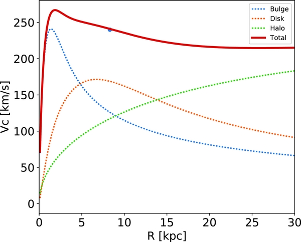
Figure 1. Total circular velocity curve and the contribution of each component associated to the axisymmetric Galactic mass model. The blue dot shows the velocity at the Sun position.
The presence of a bar in the inner regions of the Milky Way is well-known (e.g. Binney et al. Reference Binney, Gerhard, Stark, Bally and Uchida1991; Weiner & Sellwood Reference Weiner and Sellwood1999; Hammersley et al. Reference Hammersley, Garzón, Mahoney, López-Corredoira and Torres2000; Benjamin et al. Reference Benjamin2005)—see a more detailed discussion in Barbuy, Chiappini, & Gerhard (Reference Barbuy, Chiappini and Gerhard2018, and references therein). In order to go beyond a simplistic axisymmetric modelling of the central regions of the Galaxy, we added a single rotating bar to our mass model. Several models of the Galactic bar have been proposed in the past (e.g. Long & Murali Reference Long and Murali1992; Pichardo et al. Reference Pichardo, Martos and Moreno2004). In the present work, we adopted the widely used (e.g. Pfenniger Reference Pfenniger1984; Weiner & Sellwood Reference Weiner and Sellwood1999; Gardner & Flynn Reference Gardner and Flynn2010; Berentzen & Athanassoula Reference Berentzen and Athanassoula2012; Jílková et al. Reference Jílková, Carraro, Jungwiert and Minchev2012; Casetti-Dinescu et al. Reference Casetti-Dinescu2013) description in terms of a triaxial rotating Ferrer’s ellipsoid
 $$\begin{equation}
\rho _\mathrm{bar}= \left\lbrace \begin{array}{@{}l@{\quad }l@{}}\rho _{\mathrm{c}}(1-m^2)^n,\;\; & m< 1\\
0,\;\; & m\ge 1, \end{array}\right.
\end{equation}$$
$$\begin{equation}
\rho _\mathrm{bar}= \left\lbrace \begin{array}{@{}l@{\quad }l@{}}\rho _{\mathrm{c}}(1-m^2)^n,\;\; & m< 1\\
0,\;\; & m\ge 1, \end{array}\right.
\end{equation}$$
where ρc is the central density, n is a positive integer, and
 $$\begin{equation}
m^2=\frac{x^2}{a^2}+\frac{y^2}{b^2}+\frac{z^2}{c^2},
\end{equation}$$
$$\begin{equation}
m^2=\frac{x^2}{a^2}+\frac{y^2}{b^2}+\frac{z^2}{c^2},
\end{equation}$$
with a, b, and c the semi-axes of the ellipsoid. The adopted value of the parameters of the bar and the reference papers are summarised in Table 2. When adding the bar to the mass model, all the mass in the Sérsic component is employed to build the Galactic bar.
In our calculations, we neglected the presence of spiral arms perturbing the gravitational potential of the Galactic disc. The reason for this is that the clusters in our sample are confined within the inner ≃ 4 kpc of the Galaxy, which is approximately the size of the semi-major axis of the Galactic bar. We then do not expect the orbits to be perturbed by a rotating spiral pattern, which typically develops outside the volume occupied by the bar.
3.2. Integration of the orbits
We integrated the Galactic orbits of the GCs using nigo (Numerical Integrator of Galactic Orbits –Rossi Reference Rossi2015a), which is ideally suitable for the purposes of our analysis. The code includes an implementation of the mass model that we adopted in this work. The solution of the EoM is evaluated numerically using the Shampine–Gordon integration scheme [for further details, we refer to Rossi (Reference Rossi2015b)]. We integrated the orbits of our sample of star clusters forward in time for 10 Gyr. Using the observational parameters of the GCs given in Table 1, we computed the initial state vector of the clusters assuming the Sun’s Galactocentric distance R 0 = 8.33 kpc and a circular velocity V 0 = 241 km s−1 (e.g. Bland-Hawthorn & Gerhard Reference Bland-Hawthorn and Gerhard2016, and references therein). The velocity components of the Sun with respect to the local standard of rest are (U, V, W)⊙ = (11.1, 12.24, 7.25) km s−1 (Schönrich, Binney, & Dehnen Reference Schönrich, Binney and Dehnen2010). We defined as inertial Galactocentric frame of reference the right-handed system of coordinates (x, y, z) where the x-axis points to the Sun from the Galactic centre and the z-axis points to the North Galactic Pole. We refer to the bar-corotating frame of reference as the right-handed system of coordinates (x r, y r, z r) that co-rotates with the bar, where the x r axis is aligned with the bar semi-major axis a and z r points towards the North Galactic Pole. As we mention in Section 2, our proper motions are relative to the bulge field stars, therefore we have to give a special treatment in order to get the velocity vector, as was explained in Terndrup et al. (Reference Terndrup, Popowski, Gould, Rich and Sadler1998) and in Paper I. It is worth to point out that Bobylev & Bajkova (Reference Bobylev and Bajkova2017) carried out an orbital study with the same sample GCs and data from Paper I. However, they did not apply the correct conversion from relative proper motions into velocities, assuming that the proper motions given in Paper I were absolute. Therefore, their calculated velocity vectors are not consistent with this sample of bulge GCs. For NGC 6652, the proper motions are absolute, such that for this cluster we apply the usual way to convert the proper motions into velocities.
4 ORBITAL PROPERTIES OF THE BULGE GLOBULAR CLUSTERS
In this section, we present the main properties of the Galactic orbits determined for each of the nine GCs in our sample, both for the cases of an axisymmetric and a barred Galactic mass model using three different values of the angular velocity of the bar Ωb = 40, 50, and 60 km s−1 kpc−1.
Figure 2 shows the orbit for each individual GC using as initial condition the central values presented in Table 1, both in the case of the axisymmetric potential (three left panels) and the model with bar (three right panels). For each cluster, we plotted the projection of the orbit on the Galactic plane (x − y), on the (x − z) plane and on the meridional plane (R − z). The orbits obtained assuming an axisymmetric potential are shown in the inertial Galactic frame of reference, while the orbits obtained in the barred potential are shown in the bar co-rotating frame of reference. In the model with bar, we use three different angular velocities, that are plotted with different colours in the right panels of Figure 2.

Figure 2. Orbits for the sample of globular clusters. The three left columns show x–y, x–z, and R–z projections for orbits with the axisymmetric Galactic potential, while the three right columns show the orbits with the non-axisymmetric Galactic potential co-rotating with the bar. The colours in the left panels are the orbits with different pattern speed of the bar, 40 (blue), 50 (black), and 60 (grey) km s−1 kpc−1. The dashed red line shows the size of the Galactic bar.
For each orbit in Figure 2, we calculate the perigalactic distance r min, the apogalactic distance r max, the maximum vertical excursion from the Galactic plane |z|max, and the eccentricity defined as e = (r max − r min)/(r max + r min). In order to know whether the orbital motion of GCs has a prograde or a retrograde sense with respect to the rotation of the bar, we calculate the z-component of the angular momentum in the inertial frame, Lz. Since this quantity is not conserved in a model with non-axisymmetric structures, we are interested only in the sign.
We can see that with the axisymmetric potential, most of clusters are confined inside ~2 kpc in the Galactic plane, except for NGC 6540 and NGC 6652, that reach distances between ~4 and 5 kpc. The clusters have a z-distance from the Galactic plane of ~0.6, except for NGC 6558 with z ~ 1.3, and NGC 6652 with z ~ 2.6 kpc. Most of clusters show high eccentricity e > 0.8, although there are three clusters with e < 0.5 (Terzan 2, Terzan 4, and NGC 6540).
When the bar is introduced to the model, there is an interesting dynamical effect produced by this structure. In general, the clusters are confined in the bar region. For the cases of Terzan 1 and NGC 6540, these clusters are going inside and outside of the bar in the Galactic plane, with low vertical excursions from the plane. It is not surprising that NGC 6652 is also completely outside of the bar region because we know that this cluster belongs to the halo component. We can also notice that Terzan 4, Terzan 9, NGC 6522, NGC 6558, Palomar 6 have a bar-shape orbit in the (x r − y r) projection, and a boxy-shape in the (x r − z r), and this means that these clusters are trapped by the bar. NGC 6540 has a particular and different behaviour as compared with the other sample clusters: it is confined to the Galactic plane, and has the correct energy to go inside and outside of the bar, and the orbit is trapped by a higher-order resonance or corotation, depending on the bar angular velocity, Ωb. With respect to the different values of Ωb, we can see that most of orbits are not sensitive to the change of this parameter, except for NGC 6558, NGC 6540, and NGC 6652. Regarding the sense of the orbital motion, we have clusters with prograde orbits such as Terzan 4, NGC 6522, NGC 6558, NGC 6540, and we have clusters that have prograde and retrograde orbits at the same time. The prograde–retrograde clusters are Terzan 2, Terzan 9, Palomar 6 and NGC 6652. The prograde–retrograde orbits have been observed before in others GCs (Pichardo et al. Reference Pichardo, Martos and Moreno2004; Allen et al. Reference Allen, Moreno and Pichardo2006). This effect is produced by the presence of the bar, and it could be related to chaotic behaviour, however this is not well-understood yet.
4.1. Orbital properties from the Monte Carlo method
In order to evaluate the uncertainties associated with the parameters of the clusters, we followed a Monte Carlo method. For each cluster we generated a set of 1 000 initial conditions included within the errors affecting the values of heliocentric distance, proper motions and heliocentric radial velocity, presented in Table 1. We do this with the purpose of seeing how much the orbital properties of the clusters such as the perigalactic distance, the apogalactic distance, the maximum vertical height and the eccentricity change, considering the errors of the measurements, and at the same time, how the Galactic bar affects them. We integrated this set of orbits for 10 Gry using nigo and evaluated the mean value and standard deviation of the orbital parameters.
In Table 3, we give for each GC the orbital parameters obtained with the axisymmetric potential (first line) and the model with bar, where we employed three values of Ωb = 40 (second line), 50 (third line) and 60 (forth line) km s−1 kpc−1. Columns 2–4 show the average perigalactic distance, the average apogalactic distance, and the average maximum vertical excursion from the Galactic plane, respectively. Column 5 gives the average orbital eccentricity. The errors provided in each column are the standard deviation of the distribution.
Table 3. Orbital parameters with the axisymmetric and non-axisymmetric potentials.

Figure 3 shows the distribution of each orbital parameter, for the axisymmetric model (blue) and the model with bar using a Ωb = 40 (orange), 50 (green), and 60 (red) km s−1 kpc−1. The clusters have perigalactic distances r min < 1 kpc with the axisymmetric model, and these decrease with the presence of the bar,  $r_\mathrm{\text{min}}<0.5$ kpc. There is a particular cluster, NGC 6540, with perigalactic distance with the axisymmetric model between 1 and 3 kpc, and with bar model between 0.5 and 4 kpc, depending on the pattern speed. Regarding the apogalactic distance, the clusters can reach maximum distances up to 4 kpc, and there are two clusters that could go further, NGC 6540 (up to 6 kpc) and NGC 6652 (up to 8 kpc). As for the maximum height, the clusters could go between 0.5 to 1.5 kpc, and for NGC 6652 up to 5 kpc. With respect to eccentricity, most clusters have high eccentricities, and the bar model makes the distribution in eccentricities to be narrower than with the axisymmetric model. The exceptions are Terzan 4, with a low eccentricity with no bar, whereas the orbits become highly eccentric with the presence of the bar; and NGC 6540, with a very low eccentricity, e < 0.5, with the axisymmetric model, whereas with the bar model the eccentricity depends on the angular velocity, higher if Ωb > 50 km s−1 kpc−1 or lower if Ωb < 50 km s−1 kpc−1.

Figure 3. Distribution of orbital parameters for each cluster. The distribution for perigalactic r min, apogalactic r max, maximum vertical hight of orbit |z|max, and eccentricity e. Different colours show the distribution for the axisymmetric model (blue), model with bar using angular velocity Ωb = 40 (orange), 50 (green), and 60 (red) km s−1 kpc−1.
From the average values given in Table 3, we can see that the Galactic bar induces to have smaller average perigalactic distances (except for NGC 6540, Palomar 6, and NGC 6652), larger average apogalactic distances, lower vertical excursions from the Galactic plane (except for NGC 6652), and higher eccentricities (except for NGC 6540). The effect produced by different pattern speeds on the clusters are almost negligible, except for NGC 6540.
5 CORRELATIONS BETWEEN ORBITAL PARAMETERS AND CHEMICAL PROPERTIES
After determining the Galactic orbits of the clusters in our sample, we combined the information on the orbital properties with the metallicity, [Fe/H], given that we are particularly interested in evaluating any obvious dependence among them. In fact, we already know from Paper I that the spatial distribution of the GCs in the Galaxy has a strong dependence on their metallicity. We now aim to refine this analysis for the bulge clusters of the present sample.
We constructed scatter plots of the orbital parameters as function of the clusters’ metallicities. Figure 4 shows the distribution of perigalactic distance, apogalactic distance, maximum height from the Galactic plane, and orbital eccentricity of the clusters as function of their metallicity. We studied both cases of an axisymmetric model (blue stars) and a barred mass model with Ωb = 40 (orange squares), 50 (green circles), and 60 (red triangles) km s−1 kpc−1. We can see that the clusters with [Fe/H]≳ −1.0 have similar values in all orbital parameters. If we consider only the clusters with [Fe/H]<−1.0, the perigalactic distance and the height from the Galactic plane might tend to decrease with metallicity, while the apogalactic distance and eccentricity increase. NGC 6540 has a completely different behaviour in comparison with the other clusters. Also, we expect NGC 6652 ([Fe/H]~−1.0) having different orbital parameters from the rest, because it belongs to the halo component.
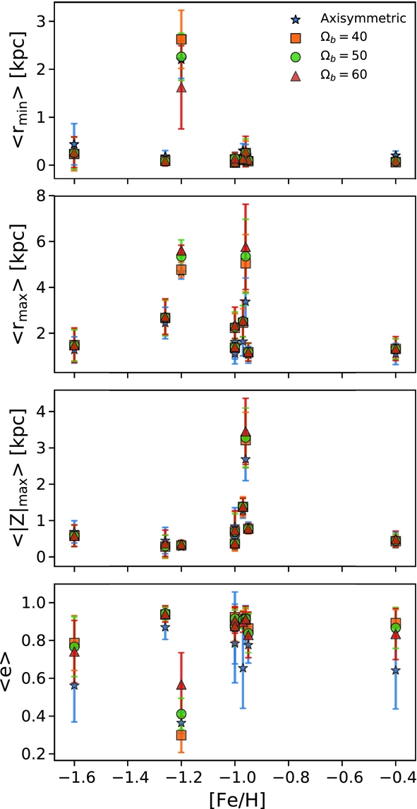
Figure 4. Scatter plots of metallicity versus orbital parameters. Read from the top. First panel: the average perigalactic distances. Second panel: the average apogalactic distances. Third panel: the average maximum excursion to the Galactic plane. Fourth panel: the average eccentricities. The blue stars show the results obtained for the axisymmetric mass model, while the orange squares, green circles, and red triangles show the results obtained for the model with bar using Ωb = 40, 50, and 60 km s−1 kpc−1, respectively.
In addition, we looked for any correlation among the different orbital parameters of the clusters. We expect the clusters sharing their dynamical properties with some dispersion, due to being confined in the bulge/bar region. In Figure 5, we show a scatter plot of all the possible combinations among the orbital parameters, where the colour represents the metallicity. We see that, in each panel, most of clusters are gathered in the same region indicating that they belong to the same component, in this case that they are confined to the bulge/bar. On the other hand, NGC 6652 and NGC 6540 have a different behaviour relative to the other ones. We know that NGC 6652 belongs to the halo component, therefore it does not have to share orbital properties with the bulge/bar GCs, and NGC 6540 has properties consistent with the thick disc kinematics.
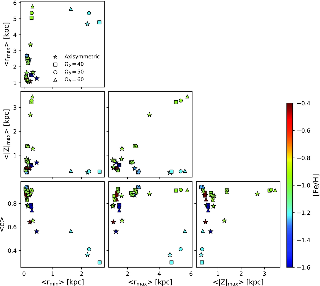
Figure 5. Orbital parameters as function of average perigalactic distance 〈r min〉, average apogalctic ditance 〈r max〉, average of maximum distance from the Galactic plane 〈|z|max〉, and average eccentricity e, for the axisymmetric model (stars), model with bar and Ωb = 40 (squares), 50 (circles), and 60 (triangles) km s−1 kpc−1. The colour bar is the cluster metallicity [Fe/H].
6 SUMMARY AND CONCLUSIONS
We have employed the available data of the bulge GCs given in Paper I to compute their orbits, and compare the orbital properties with their metallicity. This analysis has been carried out both with an axisymmetric potential and a model with the Galactic bar, where we vary the angular velocity of the bar. In order to take into account the effect of the observational uncertainties, we employed the Monte Carlo method to construct a set of 1 000 initial conditions for each cluster.
The clusters in our sample, which are projected onto the Galactic bulge, show trajectories indicating that they are confined to a bulge/bar. The only exception applies to the comparison cluster NGC 6652, which shows an orbit expected from an inner halo cluster. We found that most of clusters in the inner 4 kpc from the Galactic centre exhibit high eccentricities with close perigalactic passages. However, we also identified an object with orbital properties completely different compared with the bulge/bar and halo component, characterised by a disc-like orbit (NGC 6540), having a larger perigalactic distance larger than 5 kpc with very low eccentricities, e < 0.4. The maximum heights with respect to the Galactic plane for all the sample clusters (except for NGC 6652), are typically below 1.5 kpc. It appears that the sample clusters evolve within the region occupied by the Galactic bar. More specifically, due to the gravitational effect produced by the bar, the clusters could be trapped by some resonance of the bar, and in this case they would be those that follow a bar-shape in (x r − y r) and (x r − z r), in the rotating frame. On the other hand, the cluster Terzan 1, that even though it is confined in the inner region, its orbit does not have a bar-/boxy-shape, therefore this cluster is probably not trapped by the bar. In any case, as expected, the presence of a rotating bar in the centre of the Galaxy has a strong impact on the orbital evolution of the inner clusters, although the effect produced by different angular velocities on the clusters seems to be almost negligible, except for NGC 6540.
We found that most clusters in the inner ~3 kpc are part of the bulge/bar population. By this, we mean that either these clusters were formed early on before bar formation, and were trapped during the bar formation, or else, they formed together with the bar. On the other hand, it appears that in the region outside the bar, the clusters appear to behave as thick disk-like orbits or halo, such as NGC 6540 and NGC 6652, respectively.
With respect to metallicity correlations, the properties are similar for clusters with [Fe/H]≳ −1.0. On the other hand, if we consider only clusters with [Fe/H]<−1.0, the perigalactic distance and the maximum high excursion from the Galactic plane tend to decrease with metallicity, while the apogalactic and eccentricity increase. However, there is not any obvious dependence among the metallicity and orbital properties. We suggest that a more extensive analysis of a larger bulge cluster sample is required to improve the statistical significance of these results.
Our results could provide some insight on the formation processes of the GCs located in the Galactic bulge. Considering the old nature of these objects (e.g. Ortolani et al. Reference Ortolani, Barbuy, Momany, Saviane, Bica, Jilkova, Salerno and Jungwiert2011; Kerber et al. Reference Kerber2018), they were formed during the very early stages of the evolution of the Milky Way. Also, many of the sample clusters belong to the metal-rich Galactic sub-population (Paper I and references therein), and therefore they likely formed within high-pressure, metal-rich gas Galactic structures at high redshift.
In our analysis, we have orbits with prograde motions and orbits that change their sense of motion from prograde to retrograde, as seen from the inertial frame. The prograde–retrograde orbits could be related to the chaotic behaviour (Pichardo et al. Reference Pichardo, Martos and Moreno2004; Allen et al. Reference Allen, Moreno and Pichardo2006). The absence of strong correlations between orbital and chemical properties of the clusters could be indicative of an early chaotic phase of the evolution of the central regions of the Galaxy, as well. This is consistent with a scenario in which the bulge formed at high redshift through processes such as mergers and violent disc instabilities, as recently confirmed by Tacchella et al. (Reference Tacchella2015). On the other hand, there is evidence that the Galactic bar is relatively recent with respect to the age of the bulge clusters. Cole & Weinberg (Reference Cole and Weinberg2002), for example, concluded that the bar must be younger than 6 Gyr. In this case, the clusters formed before the development of the bar instability. An example could be NGC 6522, that is a very old cluster, ~13 Gyr (Kerber et al. Reference Kerber2018) but has a bar-/boxy-shape orbit (in the rotating frame), meaning that it was formed in a very early stage of the Galaxy, before bar formation, and it was trapped by the bar later on.
ACKNOWLEDGEMENTS
We acknowledge the anonymous referee for enlightening comments that greatly improved this paper. APV acknowledges FAPESP for the postdoctoral fellowship 2017/15893-1. LR acknowledges a CRS scholarship from Swinburne University of Technology. BB and EB acknowledge grants from the Brazilian agencies CNPq and Fapesp. SO acknowledges the Italian Ministero dell’Università e della Ricerca Scientifica e Tecnologica, the Istituto Nazionale di Astrofisica (INAF), and the financial support of the University of Padova.


