


1. Introduction
The epoch of reionisation (EoR) is a fundamental milestone in the evolution of our Universe. Its timing and spatial fluctuations encode invaluable information about the intergalactic medium (IGM) and the first galaxies. Recent years have witnessed a dramatic increase in the number and quality of observations probing the EoR, including upper limits on the cosmic 21-cm power spectrum (Mertens et al. Reference Mertens2020; Trott et al. Reference Trott2020; HERA Collaboration et al. Reference Collaboration2023), the polarisation anisotropy of the cosmic microwave background (CMB; Planck Collaboration et al. Reference Collaboration2020; Reichardt et al. Reference Reichardt2021), and the IGM Lyman- $\alpha$
(Ly
$\alpha$
(Ly $\alpha$
) damping-wing absorption seen in spectra of high-redshift quasars (Eduardo Bañados et al. Reference Bañados2018; Wang et al. Reference Wang2020) and star-forming galaxies (Pentericci et al. Reference Pentericci2018; Umeda et al. Reference Umeda, Ouchi, Nakajima, Harikane, Ono, Xu, Isobe and Zhang2024; Heintz et al. Reference Heintz2024).
$\alpha$
) damping-wing absorption seen in spectra of high-redshift quasars (Eduardo Bañados et al. Reference Bañados2018; Wang et al. Reference Wang2020) and star-forming galaxies (Pentericci et al. Reference Pentericci2018; Umeda et al. Reference Umeda, Ouchi, Nakajima, Harikane, Ono, Xu, Isobe and Zhang2024; Heintz et al. Reference Heintz2024).
Arguably the most mature of EoR datasets is the Ly $\alpha$
forest. More than two decades of observational efforts have provided over 70 high-quality quasar spectra at
$\alpha$
forest. More than two decades of observational efforts have provided over 70 high-quality quasar spectra at $z\gt5.5$
(Fan et al. Reference Fan, Narayanan, Strauss, White, Becker, Pentericci and Rix2002, Reference Fan2006b,a; Willott et al. Reference Willott2007; Becker et al. Reference Becker, Bolton, Madau, Pettini, Ryan-Weber and Venemans2015; Wu et al. Reference Wu2015; Eduardo Bañados et al. Reference Bañados2016; Jiang et al. Reference Jiang2016; Eilers, Davies, & Hennawi Reference Eilers, Davies and Hennawi2018; Yang et al. Reference Yang2020; D’Odorico et al. Reference D’Odorico2023). These data provide unparalleled statistics over large volumes of the IGM. As such, the Ly
$z\gt5.5$
(Fan et al. Reference Fan, Narayanan, Strauss, White, Becker, Pentericci and Rix2002, Reference Fan2006b,a; Willott et al. Reference Willott2007; Becker et al. Reference Becker, Bolton, Madau, Pettini, Ryan-Weber and Venemans2015; Wu et al. Reference Wu2015; Eduardo Bañados et al. Reference Bañados2016; Jiang et al. Reference Jiang2016; Eilers, Davies, & Hennawi Reference Eilers, Davies and Hennawi2018; Yang et al. Reference Yang2020; D’Odorico et al. Reference D’Odorico2023). These data provide unparalleled statistics over large volumes of the IGM. As such, the Ly $\alpha$
forest is one of the few EoR probes that is not sensitive to the biased environments proximate to the ionizing sources.
$\alpha$
forest is one of the few EoR probes that is not sensitive to the biased environments proximate to the ionizing sources.
The high quality and quantity of Lya forest data provide an invaluable stress test on our understanding of the EoR, as they are quite sensitive to missing components in our theoretical and systematic models. For instance, the observed large-scale fluctuations in the Ly $\alpha$
optical depth cannot be reproduced by the simplest, uniform ultraviolet background (UVB) models at
$\alpha$
optical depth cannot be reproduced by the simplest, uniform ultraviolet background (UVB) models at $z\gt5.2$
(Becker et al. Reference Becker, Bolton, Madau, Pettini, Ryan-Weber and Venemans2015; Bosman et al. Reference Bosman2022). Various theoretical models have attempted to reproduce the observations by increasing fluctuations in the IGM temperature, mean free path (MFP) of ionizing photons, ionizing emissivity, and/or including an ongoing, patchy reionisation (D’Aloisio, McQuinn, & Trac Reference D’Aloisio, McQuinn and Trac2015; Davies & Furlanetto Reference Davies and Furlanetto2016; D’Aloisio et al. Reference D’Aloisio, Upton Sanderbeck, McQuinn, Trac and Shapiro2017, Reference D’Aloisio, McQuinn, Davies and Furlanetto2018; Chardin, Puchwein, & Haehnelt Reference Chardin, Puchwein and Haehnelt2017; Kulkarni et al. Reference Kulkarni, Keating, Haehnelt, Bosman, Puchwein, Chardin and Aubert2019; Keating et al. Reference Keating, Weinberger, Kulkarni, Haehnelt, Chardin and Aubert2020; Meiksin Reference Meiksin2020; Nasir & D’Aloisio Reference Nasir and D’Aloisio2020; Asthana et al. Reference Asthana, Haehnelt, Kulkarni, Aubert, Bolton and Keating2024). However, moving beyond ‘this particular model is (in)consistent with the data’ to ‘this is the distribution of IGM and galaxy properties inferred from the data’ is considerably more challenging, and can only be achieved in a physically-motivated, efficient Bayesian inference framework.
$z\gt5.2$
(Becker et al. Reference Becker, Bolton, Madau, Pettini, Ryan-Weber and Venemans2015; Bosman et al. Reference Bosman2022). Various theoretical models have attempted to reproduce the observations by increasing fluctuations in the IGM temperature, mean free path (MFP) of ionizing photons, ionizing emissivity, and/or including an ongoing, patchy reionisation (D’Aloisio, McQuinn, & Trac Reference D’Aloisio, McQuinn and Trac2015; Davies & Furlanetto Reference Davies and Furlanetto2016; D’Aloisio et al. Reference D’Aloisio, Upton Sanderbeck, McQuinn, Trac and Shapiro2017, Reference D’Aloisio, McQuinn, Davies and Furlanetto2018; Chardin, Puchwein, & Haehnelt Reference Chardin, Puchwein and Haehnelt2017; Kulkarni et al. Reference Kulkarni, Keating, Haehnelt, Bosman, Puchwein, Chardin and Aubert2019; Keating et al. Reference Keating, Weinberger, Kulkarni, Haehnelt, Chardin and Aubert2020; Meiksin Reference Meiksin2020; Nasir & D’Aloisio Reference Nasir and D’Aloisio2020; Asthana et al. Reference Asthana, Haehnelt, Kulkarni, Aubert, Bolton and Keating2024). However, moving beyond ‘this particular model is (in)consistent with the data’ to ‘this is the distribution of IGM and galaxy properties inferred from the data’ is considerably more challenging, and can only be achieved in a physically-motivated, efficient Bayesian inference framework.
Previous work that reproduced the data relied heavily on effective (i.e. not physically interpretable) parameters and/or ad-hoc assumptions that ignore or fine-tune the redshift evolution of the mean transmission flux. For example, several studies found that in order to reproduce the forest data, the UV ionizing emissivity in their simulations has to be tuned to drop rapidly towards the end of the EoR, with up to a factor of 2 decrement over just $\Delta z\sim0.5$
(
$\Delta z\sim0.5$
( ${\sim}100$
Myr at these redshifts; e.g. Kulkarni et al. Reference Kulkarni, Keating, Haehnelt, Bosman, Puchwein, Chardin and Aubert2019; Ocvirk et al. Reference Ocvirk, Lewis, Gillet, Chardin, Aubert, Deparis and Thélie2021; Fig. 6). Such short time-scales for the UVB evolution are difficult to justify physically (e.g. Sobacchi & Mesinger Reference Sobacchi and Mesinger2013) or to reconcile with the observed gradual evolution of the cosmic star formation rate (SFR) density from bright galaxies (Bouwens et al. Reference Bouwens2015b; Oesch et al. Reference Oesch, Bouwens, Illingworth, Labbé and Stefanon2018). Indeed subsequent analysis pointed to unresolved substructure in the simulations as a possible explanation (e.g. see section 5.4 in Qin et al. Reference Qin, Mesinger, Bosman and Viel2021, and the recent analysis in Cain et al. Reference Cain, D’Aloisio, Lopez, Gangolli and Roth2024). Alternatively, simulations that tune the ionizing MFP without modelling the time evolution of HII regions and/or adopt effective parameters for inhomogeneous recombinations are also difficult to interpret as they only provide a somewhat opaque proxy for cosmic reionisation (e.g. Choudhury, Paranjape, & Bosman Reference Choudhury, Paranjape and Bosman2021; Gaikwad et al. Reference Gaikwad2023; Davies et al. Reference Davies2024).
${\sim}100$
Myr at these redshifts; e.g. Kulkarni et al. Reference Kulkarni, Keating, Haehnelt, Bosman, Puchwein, Chardin and Aubert2019; Ocvirk et al. Reference Ocvirk, Lewis, Gillet, Chardin, Aubert, Deparis and Thélie2021; Fig. 6). Such short time-scales for the UVB evolution are difficult to justify physically (e.g. Sobacchi & Mesinger Reference Sobacchi and Mesinger2013) or to reconcile with the observed gradual evolution of the cosmic star formation rate (SFR) density from bright galaxies (Bouwens et al. Reference Bouwens2015b; Oesch et al. Reference Oesch, Bouwens, Illingworth, Labbé and Stefanon2018). Indeed subsequent analysis pointed to unresolved substructure in the simulations as a possible explanation (e.g. see section 5.4 in Qin et al. Reference Qin, Mesinger, Bosman and Viel2021, and the recent analysis in Cain et al. Reference Cain, D’Aloisio, Lopez, Gangolli and Roth2024). Alternatively, simulations that tune the ionizing MFP without modelling the time evolution of HII regions and/or adopt effective parameters for inhomogeneous recombinations are also difficult to interpret as they only provide a somewhat opaque proxy for cosmic reionisation (e.g. Choudhury, Paranjape, & Bosman Reference Choudhury, Paranjape and Bosman2021; Gaikwad et al. Reference Gaikwad2023; Davies et al. Reference Davies2024).
Ideally, one should use a self-consistent model in which the redshift evolution of the patchy reionisation is simulated directly from the galaxies that drive it. This would allow us to set well-motivated priors on physical parameters that can be constrained by complementary galaxy observations (e.g. Park et al. Reference Park, Mesinger, Greig and Gillet2019; Mutch et al. Reference Mutch, Greig, Qin, Poole and Wyithe2024). Anchoring the EoR models on galaxies also allows us to constrain earlier epochs where we have no forest measurements, since structure evolution (i.e., the halo mass function) is comparably well understood (e.g. Sheth et al. Reference Sheth, Mo and Tormen2001) and we have complementary observations of UV luminosity functions (LFs) that constrain how halos are populated with galaxies at these high redshifts.
However, such self-consistent modelling of the EoR is inherently extremely challenging, due to the enormous dynamic range of relevant scales. Fluctuations in the Ly $\alpha$
forest are correlated on scales larger than
$\alpha$
forest are correlated on scales larger than ${\sim}100$
cMpc (e.g. Becker et al. Reference Becker, D’Aloisio, Christenson, Zhu, Worseck and Bolton2021; Zhu et al. Reference Zhu2021), while galaxies and IGM clumps are on sub-kpc scales (e.g. Schaye Reference Schaye2001; Emberson, Thomas, & Alvarez Reference Emberson, Thomas and Alvarez2013; Park et al. Reference Park and Shapiro2016; D’Aloisio Reference D’Aloisio, McQuinn, Trac, Cain and Mesinger2020). As a result, current simulations must rely on sub-grid prescriptions that have to be calibrated against observations or other more detailed, higher resolution simulations.
${\sim}100$
cMpc (e.g. Becker et al. Reference Becker, D’Aloisio, Christenson, Zhu, Worseck and Bolton2021; Zhu et al. Reference Zhu2021), while galaxies and IGM clumps are on sub-kpc scales (e.g. Schaye Reference Schaye2001; Emberson, Thomas, & Alvarez Reference Emberson, Thomas and Alvarez2013; Park et al. Reference Park and Shapiro2016; D’Aloisio Reference D’Aloisio, McQuinn, Trac, Cain and Mesinger2020). As a result, current simulations must rely on sub-grid prescriptions that have to be calibrated against observations or other more detailed, higher resolution simulations.
Here, we present an updated Bayesian inference framework for the high-redshift Ly $\alpha$
forest that is arguably free from ‘effective’ parameters. We sample physically-intuitive galaxy scaling relations to compute large-scale lightcones of the Ly
$\alpha$
forest that is arguably free from ‘effective’ parameters. We sample physically-intuitive galaxy scaling relations to compute large-scale lightcones of the Ly $\alpha$
opacity using 21cmFAST (Mesinger, Furlanetto, & Cen Reference Mesinger, Furlanetto and Cen2011; Murray et al. Reference Murray, Greig, Mesinger, Muñoz, Qin, Park and Watkinson2020). This self-consistently connects galaxy properties to the state of the IGM that is shaped by their radiation fields. We account for missing small-scale structure by calibrating to the Sherwood suite of high-resolution hydrodynamic simulations (Bolton et al. Reference Bolton, Puchwein, Sijacki, Haehnelt, Kim, Meiksin, Regan and Viel2017). This calibration allows us to eliminate the poorly-motivated hyperparameters we previously used to account for missing systematics and/or physics (Qin et al. Reference Qin, Mesinger, Bosman and Viel2021, hereafter Q21). For each astrophysical parameter combination, we forward model the forest transmission, comparing against the observations (Bosman et al. Reference Bosman2022) using an implicit likelihood. We present the resulting joint constraints on reionisation and galaxy properties, implied by the combined data from the Ly
$\alpha$
opacity using 21cmFAST (Mesinger, Furlanetto, & Cen Reference Mesinger, Furlanetto and Cen2011; Murray et al. Reference Murray, Greig, Mesinger, Muñoz, Qin, Park and Watkinson2020). This self-consistently connects galaxy properties to the state of the IGM that is shaped by their radiation fields. We account for missing small-scale structure by calibrating to the Sherwood suite of high-resolution hydrodynamic simulations (Bolton et al. Reference Bolton, Puchwein, Sijacki, Haehnelt, Kim, Meiksin, Regan and Viel2017). This calibration allows us to eliminate the poorly-motivated hyperparameters we previously used to account for missing systematics and/or physics (Qin et al. Reference Qin, Mesinger, Bosman and Viel2021, hereafter Q21). For each astrophysical parameter combination, we forward model the forest transmission, comparing against the observations (Bosman et al. Reference Bosman2022) using an implicit likelihood. We present the resulting joint constraints on reionisation and galaxy properties, implied by the combined data from the Ly $\alpha$
forest, UV LFs, and CMB optical depth.
$\alpha$
forest, UV LFs, and CMB optical depth.
This paper is organised as follows. We summarise the extended XQR-30 Ly $\alpha$
forest data in Section 2, and introduce our Bayesian framework for forward-modelling Ly
$\alpha$
forest data in Section 2, and introduce our Bayesian framework for forward-modelling Ly $\alpha$
forests in Section 3. After summarizing the complementary observations and free parameters used in this work in Sections 3.5 and 3.6, we present results in Section 4 including the recovered properties of the IGM and those of the underlying galaxies. We then discuss the implication to our understanding of reionisation in Section 5, before concluding in Section 6. In this work, we adopt cosmological parameters from Planck (
$\alpha$
forests in Section 3. After summarizing the complementary observations and free parameters used in this work in Sections 3.5 and 3.6, we present results in Section 4 including the recovered properties of the IGM and those of the underlying galaxies. We then discuss the implication to our understanding of reionisation in Section 5, before concluding in Section 6. In this work, we adopt cosmological parameters from Planck ( $\Omega_{{m}}, \Omega_{{b}}, \Omega_{\mathrm{\Lambda}}, h, \sigma_8, n_{s} $
= 0.312, 0.0490, 0.688, 0.675, 0.815, 0.968; Planck Collaboration et al. Reference Collaboration2016). Distance units are comoving unless otherwise specified.
$\Omega_{{m}}, \Omega_{{b}}, \Omega_{\mathrm{\Lambda}}, h, \sigma_8, n_{s} $
= 0.312, 0.0490, 0.688, 0.675, 0.815, 0.968; Planck Collaboration et al. Reference Collaboration2016). Distance units are comoving unless otherwise specified.
2. The Ly $\alpha$
opacity distributions from XQR-30+
$\alpha$
opacity distributions from XQR-30+

The ultimate XSHOOTER legacy survey of quasars at $z\sim5.8$
–6.6 (XQR-30) is a
$z\sim5.8$
–6.6 (XQR-30) is a ${\sim}250$
-h programme using the Very Large Telescope (VLT) at the European Southern Observatory (ESO; D’Odorico et al. Reference D’Odorico2023). While XQR-30 contains 30 high-quality quasar spectra, Bosman et al. (Reference Bosman2022) assembled 67 sightlines at these redshifts by combining XQR-30 with archival spectra. We refer to this extended dataset as XQR-30+.
${\sim}250$
-h programme using the Very Large Telescope (VLT) at the European Southern Observatory (ESO; D’Odorico et al. Reference D’Odorico2023). While XQR-30 contains 30 high-quality quasar spectra, Bosman et al. (Reference Bosman2022) assembled 67 sightlines at these redshifts by combining XQR-30 with archival spectra. We refer to this extended dataset as XQR-30+.
The Ly $\alpha$
transmission in these spectra was quantified by the commonly-used ‘effective optical depth’,
$\alpha$
transmission in these spectra was quantified by the commonly-used ‘effective optical depth’, $\tau_\textrm{eff} \equiv - \ln \langle\mathcal{F}_\alpha\rangle_{\Delta z=0.1}$
. Here
$\tau_\textrm{eff} \equiv - \ln \langle\mathcal{F}_\alpha\rangle_{\Delta z=0.1}$
. Here $\mathcal{F}_\alpha(\lambda)$
is the continuum-normalised flux in the Ly
$\mathcal{F}_\alpha(\lambda)$
is the continuum-normalised flux in the Ly $\alpha$
forest, which is averaged over segments of width
$\alpha$
forest, which is averaged over segments of width $\Delta z=0.1$
(roughly corresponding to
$\Delta z=0.1$
(roughly corresponding to $\sim$
40 cMpc at these redshifts). Non-detections (2
$\sim$
40 cMpc at these redshifts). Non-detections (2 $\sigma$
) were assigned lower limits on
$\sigma$
) were assigned lower limits on $\tau_\textrm{eff}$
corresponding to twice the mean flux noise in the corresponding segment. The full XQR-30+ sample has at least
$\tau_\textrm{eff}$
corresponding to twice the mean flux noise in the corresponding segment. The full XQR-30+ sample has at least ${\sim}10$
estimates of
${\sim}10$
estimates of $\tau_\textrm{eff}$
in each redshift bin spanning
$\tau_\textrm{eff}$
in each redshift bin spanning $z=5.1$
, 5.2, …, 6.1. We show the cumulative distribution functions (CDFs) of these
$z=5.1$
, 5.2, …, 6.1. We show the cumulative distribution functions (CDFs) of these $\tau_\textrm{eff}$
estimates in Fig. 3, where we also compare them to our fiducial posterior. For more details on how the observations were processed, see Bosman et al. (Reference Bosman2022).
$\tau_\textrm{eff}$
estimates in Fig. 3, where we also compare them to our fiducial posterior. For more details on how the observations were processed, see Bosman et al. (Reference Bosman2022).
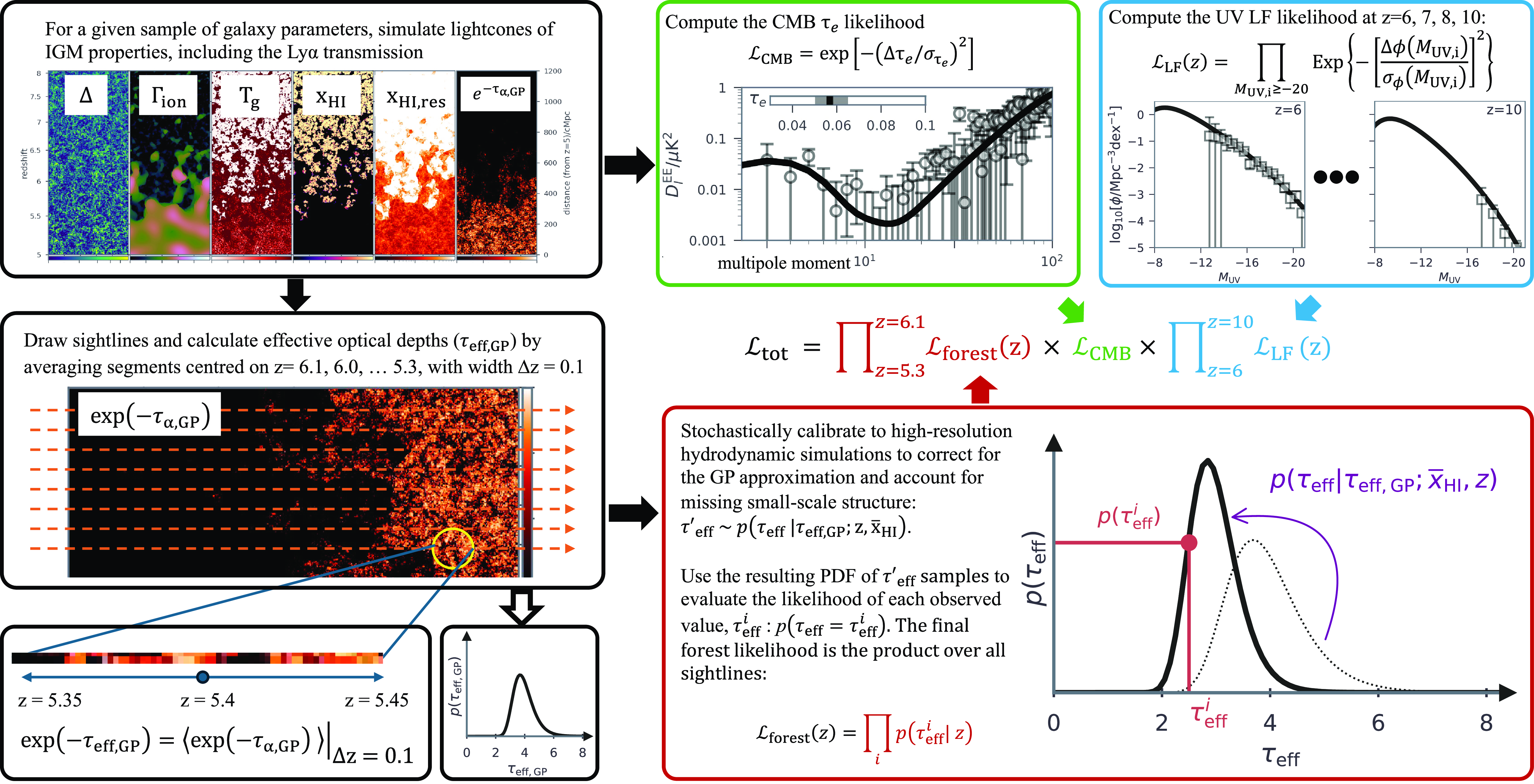
Figure 1. A flow chart showing the steps involved in computing the likelihood for a single sample of astrophysical parameters. See text for more details.
3. Forward modelling
We use the public simulation code, 21cmFAST
Footnote
a
(Mesinger & Furlanetto Reference Mesinger and Furlanetto2007; Mesinger, Furlanetto, & Cen Reference Mesinger, Furlanetto and Cen2011; Murray et al. Reference Murray, Greig, Mesinger, Muñoz, Qin, Park and Watkinson2020), to compute 3D lightcones of the Ly $\alpha$
IGM opacity. A single forward model and the corresponding likelihood evaluation are summarised in the flow chart of Fig. 1 and consist of the following steps:
$\alpha$
IGM opacity. A single forward model and the corresponding likelihood evaluation are summarised in the flow chart of Fig. 1 and consist of the following steps:
-
1. Simulate large-scale 3D lightcones of the IGM density (
$\Delta\equiv\rho/\overline{\rho}$
), neutral fraction due to inhomogeneous reionisation (
$x_\textrm{HI}$
), photo-ionisation rate (
$\Gamma_\textrm{ion}$
), IGM temperature (
$T_\textrm{g}$
), residual neutral fraction inside the ionised IGM (
$x_\textrm{HI,res}$
) and corresponding Ly
$\alpha$
opacity (top left panel of Fig. 1); -
2. Construct mock quasar sightlines and compute the effective optical depth by binning the sightlines over the same redshift intervals as the XQR-30+ observation (lower left panels of Fig. 1);
-
3. Account for missing small scales by calibrating these effective optical depths against high-resolution hydrodynamic simulations. Use the resulting probability density function (PDF) of calibrated
$\tau_\textrm{eff}$
to evaluate the likelihood of the observed values (lower right panel of Fig. 1); -
4. Multiply this forest likelihood with the corresponding UV LF and CMB likelihoods in order to obtain the total likelihood of this parameter sample (upper right panels in Fig. 1; c.f. Section 3.5).


We discuss this procedure in detail below, emphasizing the improvements over our previous analysis in Q21.
3.1 Galaxy models
Our galaxy models are based on the semi-empirical parametrisation in Park et al. (Reference Park, Mesinger, Greig and Gillet2019). We assume power laws relating the fraction of galactic baryons in stars ( $f_*$
) and the UV ionizing escape fraction (
$f_*$
) and the UV ionizing escape fraction ( $f_\textrm{esc}$
) to the host halo mass (
$f_\textrm{esc}$
) to the host halo mass ( $M_\textrm{vir}$
):
$M_\textrm{vir}$
):
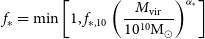 \begin{equation} f_* = \min\left[1, f_{*,10}\left(\frac{M_\textrm{vir}}{10^{10}\mathrm{M_\odot}}\right)^{\alpha_*}\right]\end{equation}
and
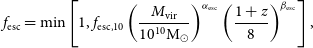 \begin{equation} f_\textrm{esc} = \min\left[1, f_\textrm{esc,10}\left(\frac{M_\textrm{vir}}{10^{10}\mathrm{M_\odot}}\right)^{\alpha_\textrm{esc}}\left(\frac{1+z}{8}\right)^{\beta_\textrm{esc}}\right],\end{equation}
where $f_{*,10}$
,
$f_{*,10}$
, $\alpha_*$
,
$\alpha_*$
, $f_\textrm{esc,10}$
,
$f_\textrm{esc,10}$
, ${\alpha_\textrm{esc}}$
and
${\alpha_\textrm{esc}}$
and ${\beta_\textrm{esc}}$
are free parameters. Compared to Park et al. (Reference Park, Mesinger, Greig and Gillet2019) and our previous analysis in Q21, here we allow for an additional redshift dependence of
${\beta_\textrm{esc}}$
are free parameters. Compared to Park et al. (Reference Park, Mesinger, Greig and Gillet2019) and our previous analysis in Q21, here we allow for an additional redshift dependence of $f_\textrm{esc}$
at a given halo mass through the parameter
$f_\textrm{esc}$
at a given halo mass through the parameter $\beta_\textrm{esc}$
(e.g. Haardt & Madau Reference Haardt and Madau2012; Kuhlen & Faucher-Giguère Reference Kuhlen and Faucher-Giguère2012; Mutch et al. Reference Mutch, Geil, Poole, Angel, Duffy, Mesinger and Wyithe2016). Note that
$\beta_\textrm{esc}$
(e.g. Haardt & Madau Reference Haardt and Madau2012; Kuhlen & Faucher-Giguère Reference Kuhlen and Faucher-Giguère2012; Mutch et al. Reference Mutch, Geil, Poole, Angel, Duffy, Mesinger and Wyithe2016). Note that $f_*$
and
$f_*$
and $f_\textrm{esc}$
have to be in the range from zero to unity as they are fractions.
$f_\textrm{esc}$
have to be in the range from zero to unity as they are fractions.
The average SFRs of galaxies over the past 100 Myr are computed as SFR = ${M_\ast}/\left[\tau_\ast H^{-1}(z)\right]$
, where
${M_\ast}/\left[\tau_\ast H^{-1}(z)\right]$
, where $M_\ast\ \equiv\ f_\ast M_\textrm{vir} {\Omega_{\mathrm{b}}}/{\Omega_{\mathrm{m}}}$
is the stellar mass, and
$M_\ast\ \equiv\ f_\ast M_\textrm{vir} {\Omega_{\mathrm{b}}}/{\Omega_{\mathrm{m}}}$
is the stellar mass, and $\tau_\ast$
is an additional free parameter corresponding to the characteristic star formation time-scale in units of the Hubble time,
$\tau_\ast$
is an additional free parameter corresponding to the characteristic star formation time-scale in units of the Hubble time, $H^{-1}(z)$
, which scales as the halo dynamical time during matter domination. Note that the 1 500 Å rest-frame luminosity used in photometric UV LF observations is sensitive to star formation over the previous 100Myr (e.g., Flores Velázquez et al. Reference Flores Velázquez2021). When forward-modeling UV LFs, we adopt the conversion factor,
$H^{-1}(z)$
, which scales as the halo dynamical time during matter domination. Note that the 1 500 Å rest-frame luminosity used in photometric UV LF observations is sensitive to star formation over the previous 100Myr (e.g., Flores Velázquez et al. Reference Flores Velázquez2021). When forward-modeling UV LFs, we adopt the conversion factor, $L_\textrm{UV}/\textrm{SFR} = 8.7\times 10^{27} \textrm{erg}\ \textrm{s}^{-1}\ \textrm{Hz}^{-1}\ \textrm{M}_\odot^{-1} \textrm{yr}$
(e.g. Madau & Dickinson Reference Madau and Dickinson2014).
$L_\textrm{UV}/\textrm{SFR} = 8.7\times 10^{27} \textrm{erg}\ \textrm{s}^{-1}\ \textrm{Hz}^{-1}\ \textrm{M}_\odot^{-1} \textrm{yr}$
(e.g. Madau & Dickinson Reference Madau and Dickinson2014).
We also assume only a fraction $f_\textrm{duty}\equiv\exp[ \def\negativespace{}-M_\textrm{turn}/M_\textrm{vir}] $
of halos host star-forming galaxies. Here,
$f_\textrm{duty}\equiv\exp[ \def\negativespace{}-M_\textrm{turn}/M_\textrm{vir}] $
of halos host star-forming galaxies. Here, $M_\textrm{turn}$
characterises the halo mass below which star formation becomes inefficient due to feedback and/or atomic cooling limits and is left as a free parameter.
$M_\textrm{turn}$
characterises the halo mass below which star formation becomes inefficient due to feedback and/or atomic cooling limits and is left as a free parameter.
Table 1. Posterior distribution ([16, 84]th percentiles) and Bayesian evidence of the galaxy models used in this work. The Bayes ratio indicates a very strong preference for the $\texttt{Evolving_f}_\texttt{esc}$
model, according to Jeffrey’s scale (e.g. Jeffreys Reference Jeffreys1939).
$\texttt{Evolving_f}_\texttt{esc}$
model, according to Jeffrey’s scale (e.g. Jeffreys Reference Jeffreys1939).
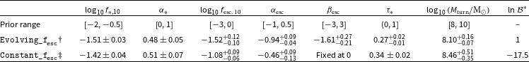
*Bayes ratio w.r.t. $\texttt{Evolving_f}_\texttt{esc}$
in natural logarithmic scale.
$\texttt{Evolving_f}_\texttt{esc}$
in natural logarithmic scale. $\dagger$
Galaxies have a mass-dependent and time-evolving escape fraction.
$\dagger$
Galaxies have a mass-dependent and time-evolving escape fraction. $\ddagger$
Galaxies have a mass-dependent and time-independent escape fraction.
$\ddagger$
Galaxies have a mass-dependent and time-independent escape fraction.
Below we explore two galaxy models, differing in their treatment of the ionizing escape fraction:
-
1.
$\texttt{Constant_f}_\texttt{esc}$
– the ionizing escape fraction is a function of halo mass only and is constant with redshift (fixing
${\beta_\textrm{esc}}$
to zero in equation 2). Note that this model does effectively allow for the population-averaged escape fraction to evolve with redshift, since
$f_\textrm{esc}$
depends on halo mass and the halo mass function evolves with redshift. This sets a ‘characteristic’ halo mass that drives both the timing and morphology of reionisation. -
2.
$\texttt{Evolving_f}_\texttt{esc}$
– the ionizing escape fraction is a function of halo mass and evolves with redshift (treating both
${\alpha_\textrm{esc}}$
and
${\beta_\textrm{esc}}$
as free parameters in equation 2). Note that adding an explicit redshift dependence to the escape fraction at a fixed halo mass gives the
$\texttt{Evolving_f}_\texttt{esc}$
model the flexibility to decouple the EoR/UVB morphology from the mean EoR history.


In this work we perform inference with both models, comparing their Bayesian evidences. We find that the data strongly prefer $\texttt{Evolving_f}_\texttt{esc}$
, and we therefore refer to this model as ‘fiducial’. We list the posterior distribution and Bayesian evidence of these two models in Table 1.
$\texttt{Evolving_f}_\texttt{esc}$
, and we therefore refer to this model as ‘fiducial’. We list the posterior distribution and Bayesian evidence of these two models in Table 1.
3.2 Large-scale IGM simulations
Our simulation boxes are 250 cMpc on a side. Realisations of Gaussian initial conditions are computed at $z=300$
on a 640
$z=300$
on a 640 $^3$
grid, with the density fields evolved down to
$^3$
grid, with the density fields evolved down to $z=5$
using second order Lagrangian perturbation theory (2LPT; Scoccimarro Reference Scoccimarro1998) and smoothed down to a final resolution of 128
$z=5$
using second order Lagrangian perturbation theory (2LPT; Scoccimarro Reference Scoccimarro1998) and smoothed down to a final resolution of 128 $^3$
. Galaxy abundances are identified from the evolved density fields using excursion-set theory (Mesinger, Furlanetto, & Cen Reference Mesinger, Furlanetto and Cen2011), and assigned properties including the stellar mass, SFR, ionizing escape fraction and duty cycle according to the galaxy models discussed in the previous section.
$^3$
. Galaxy abundances are identified from the evolved density fields using excursion-set theory (Mesinger, Furlanetto, & Cen Reference Mesinger, Furlanetto and Cen2011), and assigned properties including the stellar mass, SFR, ionizing escape fraction and duty cycle according to the galaxy models discussed in the previous section.
Reionisation is modeled with the excursion-set approach (Furlanetto, Zaldarriaga, & Hernquist Reference Furlanetto, Zaldarriaga and Hernquist2004), accounting for inhomogeneous recombinations (Sobacchi & Mesinger Reference Sobacchi and Mesinger2014). Unlike Q21, here we include a correction for photon-conservation (Park, Greig, & Mesinger Reference Park, Greig and Mesinger2022), which further decreases the need for the nuisance hyperparameters used in our previous work. Specifically, a cell is flagged as ionised when the cumulative number of ionizing photons per baryon reaching it:
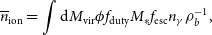 \begin{equation} \overline{n}_\textrm{ion} = \int \textrm{d}M_\textrm{vir} \phi f_\textrm{duty} M_* f_\textrm{esc} n_{\gamma} \rho_{b}^{-1},\end{equation}
exceeds the cumulative number of recombinations per baryon ( $\overline{n}_\textrm{rec}$
; accounting for unresolved substructure with the analytic framework of Sobacchi & Mesinger Reference Sobacchi and Mesinger2014):
$\overline{n}_\textrm{rec}$
; accounting for unresolved substructure with the analytic framework of Sobacchi & Mesinger Reference Sobacchi and Mesinger2014):
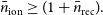 \begin{equation}\bar{n}_\textrm{ion} \geq (1 + \bar{n}_\textrm{rec}) .\end{equation}
In the above equations, $\phi$
,
$\phi$
, $n_{\gamma}$
and
$n_{\gamma}$
and $\rho_{b}$
represent the conditional halo mass function, number of ionizing photons per stellar baryon which we fix at 5 000, and baryon density. The averaging is performed over spherical regions around each cell for radii
$\rho_{b}$
represent the conditional halo mass function, number of ionizing photons per stellar baryon which we fix at 5 000, and baryon density. The averaging is performed over spherical regions around each cell for radii $R \leq R_\textrm{MFP, LLS}$
. Here
$R \leq R_\textrm{MFP, LLS}$
. Here $R_\textrm{MFP, LLS}$
corresponds to the MFP through the ionised IGM and is governed by damped Ly
$R_\textrm{MFP, LLS}$
corresponds to the MFP through the ionised IGM and is governed by damped Ly $\alpha$
systems (DLAs), Lyman limit systems (LLSs) and other unresolved systems with lower column densities (Nasir et al. Reference Nasir, Cain, D’Aloisio, Gangolli and McQuinn2021; Feron et al. Reference Feron, Conaboy, Bolton, Chapman, Haehnelt, Keating, Kulkarni and Puchwein2024; Georgiev, Mellema, & Giri Reference Georgiev, Mellema and Giri2024)
$\alpha$
systems (DLAs), Lyman limit systems (LLSs) and other unresolved systems with lower column densities (Nasir et al. Reference Nasir, Cain, D’Aloisio, Gangolli and McQuinn2021; Feron et al. Reference Feron, Conaboy, Bolton, Chapman, Haehnelt, Keating, Kulkarni and Puchwein2024; Georgiev, Mellema, & Giri Reference Georgiev, Mellema and Giri2024)
Before the end of the EoR, the total MFP determining the local ionizing background is set by a combination of $R_\textrm{MFP, LLS}$
and the distance to the surrounding neutral IGM,
$R_\textrm{MFP, LLS}$
and the distance to the surrounding neutral IGM, $R_\textrm{MFP, EoR}$
, i.e.
$R_\textrm{MFP, EoR}$
, i.e. $R_\textrm{MFP}^{-1} = R_\textrm{MFP, LLS}^{-1} + R_\textrm{MFP, EoR}^{-1}$
(e.g. Alvarez & Abel Reference Alvarez and Abel2012). The reionisation topology computed with our excursion-set algorithm determines the local (inhomogeneous)
$R_\textrm{MFP}^{-1} = R_\textrm{MFP, LLS}^{-1} + R_\textrm{MFP, EoR}^{-1}$
(e.g. Alvarez & Abel Reference Alvarez and Abel2012). The reionisation topology computed with our excursion-set algorithm determines the local (inhomogeneous) $R_\textrm{MFP, EoR}$
around each cell. However, since we do not directly resolve the spatial distribution of LSSs and DLAs when these become rare/biased, we assume a homogeneous value for
$R_\textrm{MFP, EoR}$
around each cell. However, since we do not directly resolve the spatial distribution of LSSs and DLAs when these become rare/biased, we assume a homogeneous value for $R_\textrm{MFP, LLS}=66\left[\left(1+z\right)/6.3\right]^{-4.3}$
cMpc at
$R_\textrm{MFP, LLS}=66\left[\left(1+z\right)/6.3\right]^{-4.3}$
cMpc at $z\leq6$
motivated by post-EoR measurements (Worseck et al. Reference Worseck2014; see also Songaila & Cowie Reference Songaila and Cowie2010 and Becker et al. Reference Becker, D’Aloisio, Christenson, Zhu, Worseck and Bolton2021).Footnote
b
In future work we will expand our model to additionally sample the mean and variance of
$z\leq6$
motivated by post-EoR measurements (Worseck et al. Reference Worseck2014; see also Songaila & Cowie Reference Songaila and Cowie2010 and Becker et al. Reference Becker, D’Aloisio, Christenson, Zhu, Worseck and Bolton2021).Footnote
b
In future work we will expand our model to additionally sample the mean and variance of $R_\textrm{MFP, LLS}$
, allowing us to extend our analysis to even lower redshifts.
$R_\textrm{MFP, LLS}$
, allowing us to extend our analysis to even lower redshifts.
With the above, we compute the local photoionisation rate as
 \begin{equation} {\Gamma}_\textrm{ion} = (1+z)^2 R_\textrm{MFP}\sigma_\textrm{H}\frac{\alpha_\textrm{UVB}}{\alpha_\textrm{UVB}+\beta_\textrm{H}} \! \times\! \int\! \textrm{d}M_\textrm{vir} \phi f_\textrm{duty}\frac{M_\ast}{\tau_\ast H^{-1}} f_\textrm{esc} n_{\gamma}m_p^{-1}\end{equation}
where $m_p$
is the proton mass,
$m_p$
is the proton mass, $\alpha_\textrm{UVB}=2$
corresponds to the effective spectral index of the UVB (see Becker & Bolton Reference Becker and Bolton2013; D’Aloisio et al. Reference D’Aloisio, McQuinn, Maupin, Davies, Trac, Fuller and Upton Sanderbeck2019),
$\alpha_\textrm{UVB}=2$
corresponds to the effective spectral index of the UVB (see Becker & Bolton Reference Becker and Bolton2013; D’Aloisio et al. Reference D’Aloisio, McQuinn, Maupin, Davies, Trac, Fuller and Upton Sanderbeck2019), $\beta_\textrm{H}=2.75$
and
$\beta_\textrm{H}=2.75$
and $\sigma_\textrm{H}=6.3\times10^{-18}\textrm{cm}^2$
characterise the photo-ionisation cross-section
$\sigma_\textrm{H}=6.3\times10^{-18}\textrm{cm}^2$
characterise the photo-ionisation cross-section $\sigma(\nu) =\sigma_\textrm{H} \left(\frac{\nu}{\nu_\textrm{H}}\right)^{\beta_\textrm{H}} $
with
$\sigma(\nu) =\sigma_\textrm{H} \left(\frac{\nu}{\nu_\textrm{H}}\right)^{\beta_\textrm{H}} $
with $\nu_\textrm{H}$
corresponding to the Lyman limit. After a cell is ionised, its residual neutral fraction is determined assuming photo-ionisation equilibrium:
$\nu_\textrm{H}$
corresponding to the Lyman limit. After a cell is ionised, its residual neutral fraction is determined assuming photo-ionisation equilibrium:
 \begin{equation} x_\textrm{HI, res} f_\textrm{ion,ss}\Gamma_\textrm{ion} = \chi_\textrm{HeII} \Delta\overline{n}_\textrm{H} (1-x_\textrm{HI, res})^2\alpha_\textrm{B}\end{equation}
where $\overline{n}_\textrm{H}$
is the mean hydrogen number density while
$\overline{n}_\textrm{H}$
is the mean hydrogen number density while $\Delta$
is the cell’s overdensity,
$\Delta$
is the cell’s overdensity, $\chi_\textrm{HeII}\sim1.08$
accounts for singly ionised helium,
$\chi_\textrm{HeII}\sim1.08$
accounts for singly ionised helium, $\alpha_\textrm{B}$
is the case-B recombination coefficient, and
$\alpha_\textrm{B}$
is the case-B recombination coefficient, and $f_\textrm{ion,ss}$
accounts for gas self-shielding (Rahmati et al. Reference Rahmati and Pawlik2013; see also Chardin, Kulkarni, & Haehnelt Reference Chardin, Kulkarni and Haehnelt2018). Note that sub-grid physics are implemented (Sobacchi & Mesinger Reference Sobacchi and Mesinger2014) when calculating recombinations with the sub-grid density unresolved by our simulation cells assumed to follow a volume-weighted distribution of
$f_\textrm{ion,ss}$
accounts for gas self-shielding (Rahmati et al. Reference Rahmati and Pawlik2013; see also Chardin, Kulkarni, & Haehnelt Reference Chardin, Kulkarni and Haehnelt2018). Note that sub-grid physics are implemented (Sobacchi & Mesinger Reference Sobacchi and Mesinger2014) when calculating recombinations with the sub-grid density unresolved by our simulation cells assumed to follow a volume-weighted distribution of $P_\textrm{V}(\Delta_\textrm{sub}, z)$
from Miralda-Escudé, Haehnelt, & Rees (Reference Miralda-Escudé, Haehnelt and Rees2000). However, we use the cell’s mean overdensity when computing the Ly
$P_\textrm{V}(\Delta_\textrm{sub}, z)$
from Miralda-Escudé, Haehnelt, & Rees (Reference Miralda-Escudé, Haehnelt and Rees2000). However, we use the cell’s mean overdensity when computing the Ly $\alpha$
optical depth, which neglects unresolved opacity fluctuations when calibrating to the hydrodynamic simulations below. This will be improved in future work.
$\alpha$
optical depth, which neglects unresolved opacity fluctuations when calibrating to the hydrodynamic simulations below. This will be improved in future work.
The IGM temperature ( $T_\textrm{g}$
) is tracked following McQuinn & Upton Sanderbeck (Reference McQuinn and Upton Sanderbeck2016):
$T_\textrm{g}$
) is tracked following McQuinn & Upton Sanderbeck (Reference McQuinn and Upton Sanderbeck2016):
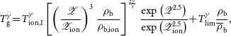 \begin{equation}T_\textrm{g}^{\gamma} {=} T_\textrm{ion,I}^{\gamma} \left[\left(\frac{\mathscr{Z}}{\mathscr{Z}_\textrm{ion}}\right)^{3} \frac{\rho_\textrm{b}}{\rho_\textrm{b,ion}}\right]^{\frac{2\gamma}{3}} \frac{\exp\left(\mathscr{Z}^{2.5}\right)}{\exp\left(\mathscr{Z}_\textrm{ion}^{2.5}\right)} {+} T_\textrm{lim}^{\gamma}\frac{\rho_\textrm{b}}{\overline{\rho}_\textrm{b}},\end{equation}
where we denote $\mathscr{Z}=(1+z)/7.1$
and use the subscript ‘
$\mathscr{Z}=(1+z)/7.1$
and use the subscript ‘ $_\textrm{ion}$
’ to indicate values at the time the cell was first ionised for convenience.
$_\textrm{ion}$
’ to indicate values at the time the cell was first ionised for convenience. $\gamma = 1.7$
is the equation of state index while
$\gamma = 1.7$
is the equation of state index while $T_\textrm{lim}=1.8\mathscr{Z}\times10^{4}$
K (Hui & Gnedin Reference Hui and Gnedin1997; Theuns et al. Reference Theuns, Leonard, Efstathiou, Pearce and Thomas1998; Puchwein et al. Reference Puchwein, Bolton, Haehnelt, Madau, Becker and Haardt2015) and
$T_\textrm{lim}=1.8\mathscr{Z}\times10^{4}$
K (Hui & Gnedin Reference Hui and Gnedin1997; Theuns et al. Reference Theuns, Leonard, Efstathiou, Pearce and Thomas1998; Puchwein et al. Reference Puchwein, Bolton, Haehnelt, Madau, Becker and Haardt2015) and $T_\textrm{ion,I}=2\times10^4$
K (D’Aloisio et al. Reference D’Aloisio, McQuinn, Maupin, Davies, Trac, Fuller and Upton Sanderbeck2019) are the relaxation and post I-front temperatures, respectively. Note that the scatter in
$T_\textrm{ion,I}=2\times10^4$
K (D’Aloisio et al. Reference D’Aloisio, McQuinn, Maupin, Davies, Trac, Fuller and Upton Sanderbeck2019) are the relaxation and post I-front temperatures, respectively. Note that the scatter in $T_\textrm{ion,I}$
has a negligible impact on the Ly
$T_\textrm{ion,I}$
has a negligible impact on the Ly $\alpha$
forest (e.g. Davies et al. Reference Davies, Mutch, Qin, Mesinger, Poole and Wyithe2019).
$\alpha$
forest (e.g. Davies et al. Reference Davies, Mutch, Qin, Mesinger, Poole and Wyithe2019).
Finally, we compute the associated Ly $\alpha$
optical depth of each 1.95 cMpc simulation cell using a form of the Fluctuating Gunn-Peterson Approximation (FGPA; Gunn & Peterson Reference Gunn and Peterson1965;Weinberg et al. Reference Weinberg, Banday, Sheth and da Costa1999) for ionised cells:
$\alpha$
optical depth of each 1.95 cMpc simulation cell using a form of the Fluctuating Gunn-Peterson Approximation (FGPA; Gunn & Peterson Reference Gunn and Peterson1965;Weinberg et al. Reference Weinberg, Banday, Sheth and da Costa1999) for ionised cells:
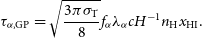 \begin{equation} \tau_{\alpha, \textrm{GP}} = \sqrt{\frac{3\pi\sigma_\textrm{T}}{8}} f_{\alpha} \lambda_\alpha c H^{-1} n_\textrm{H} x_\textrm{HI}.\end{equation}
Here $\sigma_\textrm{T}$
,
$\sigma_\textrm{T}$
, $f_\alpha{=}0.416$
,
$f_\alpha{=}0.416$
, $\lambda_\alpha{=}$
1 216 Å and
$\lambda_\alpha{=}$
1 216 Å and $n_\textrm{H}$
are the Thomson cross-section, Ly
$n_\textrm{H}$
are the Thomson cross-section, Ly $\alpha$
oscillator strength, Ly
$\alpha$
oscillator strength, Ly $\alpha$
rest-frame wavelength, and hydrogen number density, respectively. Finally, we compute the effective optical depth,
$\alpha$
rest-frame wavelength, and hydrogen number density, respectively. Finally, we compute the effective optical depth, $\tau_\textrm{eff, GP}$
, following the same definition as the observation (see Section 2).
$\tau_\textrm{eff, GP}$
, following the same definition as the observation (see Section 2).
The FGPA approximates the cross-section of Ly $\alpha$
absorption as a Dirac delta function at resonance and ignores peculiar velocities of the gas. In the following section we discuss how we use high-resolution hydrodynamic simulations to correct for the FGPA, accounting for missing small-scale structure. This represents the main improvement of this work over our previous analysis in Q21.
$\alpha$
absorption as a Dirac delta function at resonance and ignores peculiar velocities of the gas. In the following section we discuss how we use high-resolution hydrodynamic simulations to correct for the FGPA, accounting for missing small-scale structure. This represents the main improvement of this work over our previous analysis in Q21.
3.3 Accounting for missing small-scale structure
As mentioned above, our large-scale IGM simulations have a cell size of 1.95 cMpc. This is a factor of few larger than the typical Jeans length in the ionised IGM and the width of the Ly $\alpha$
cross-section at resonance. As a result, we use the FGPA in equation (8) instead of directly integrating over the full Voigt profile for the Ly
$\alpha$
cross-section at resonance. As a result, we use the FGPA in equation (8) instead of directly integrating over the full Voigt profile for the Ly $\alpha$
cross-section,
$\alpha$
cross-section, $\sigma_{\alpha}$
, and accounting for gas peculiar velocities:
$\sigma_{\alpha}$
, and accounting for gas peculiar velocities:
 \begin{equation} \tau_{\alpha}= \int \frac{\textrm{d}z}{1+z} c H^{-1} n_\textrm{H}x_\textrm{HI} \sigma_{\alpha}.\end{equation}
Does this approximation impact our modelled $\tau_\textrm{eff}$
distributions?
$\tau_\textrm{eff}$
distributions?
The fact that $\tau_\textrm{eff}$
is defined over
$\tau_\textrm{eff}$
is defined over $\Delta z =0.1$
(corresponding to roughly 20 of our IGM simulation cells) would suggest that this summary statistic is mostly sensitive to (resolved) large-scale fluctuations in flux. However, not resolving small-scale structures can effectively alias power towards large scales (e.g. Viel et al. Reference Viel, Lesgourgues, Haehnelt, Matarrese and Riotto2005; Kooistra, Lee, & Horowitz Reference Kooistra, Lee and Horowitz2022). Here we use a high-resolution hydrodynamic simulation from the Sherwood suite (Bolton et al. Reference Bolton, Puchwein, Sijacki, Haehnelt, Kim, Meiksin, Regan and Viel2017) to compare
$\Delta z =0.1$
(corresponding to roughly 20 of our IGM simulation cells) would suggest that this summary statistic is mostly sensitive to (resolved) large-scale fluctuations in flux. However, not resolving small-scale structures can effectively alias power towards large scales (e.g. Viel et al. Reference Viel, Lesgourgues, Haehnelt, Matarrese and Riotto2005; Kooistra, Lee, & Horowitz Reference Kooistra, Lee and Horowitz2022). Here we use a high-resolution hydrodynamic simulation from the Sherwood suite (Bolton et al. Reference Bolton, Puchwein, Sijacki, Haehnelt, Kim, Meiksin, Regan and Viel2017) to compare $\tau_{\textrm{eff}, \textrm{GP}}$
obtained from the low-resolution FGPA (equation 8) against the correct calculation (equation 9).
$\tau_{\textrm{eff}, \textrm{GP}}$
obtained from the low-resolution FGPA (equation 8) against the correct calculation (equation 9).
We use a simulation with a cubic volume of $80h^{-1}$
cMpc on a side and
$80h^{-1}$
cMpc on a side and $2\times512^3$
particles. It was performed using an updated version of Gadget-2 (Springel et al. Reference Springel2005) and with a slightly different
$2\times512^3$
particles. It was performed using an updated version of Gadget-2 (Springel et al. Reference Springel2005) and with a slightly different $\Lambda$
CDM cosmology (
$\Lambda$
CDM cosmology ( $\Omega_{{m}}, \Omega_{{b}}, \Omega_{\mathrm{\Lambda}}, h, \sigma_8, n_s $
= 0.31, 0.048, 0.69, 0.68, 0.83, 0.96; Planck Collaboration et al. Reference Collaboration2016). The modelled universe is exposed to a Haardt & Madau (Reference Haardt and Madau2012) UVB switched on at
$\Omega_{{m}}, \Omega_{{b}}, \Omega_{\mathrm{\Lambda}}, h, \sigma_8, n_s $
= 0.31, 0.048, 0.69, 0.68, 0.83, 0.96; Planck Collaboration et al. Reference Collaboration2016). The modelled universe is exposed to a Haardt & Madau (Reference Haardt and Madau2012) UVB switched on at $z=15$
. Although this homogeneous UVB does not account for the effects of patchy reionisation, the simulated Ly
$z=15$
. Although this homogeneous UVB does not account for the effects of patchy reionisation, the simulated Ly $\alpha$
forests from Sherwood, which has a spatial resolution of <60 kpc, agree very well with observational data at
$\alpha$
forests from Sherwood, which has a spatial resolution of <60 kpc, agree very well with observational data at $z\le5$
(Viel et al. Reference Viel, Becker, Bolton and Haehnelt2013; Bolton et al. Reference Bolton, Puchwein, Sijacki, Haehnelt, Kim, Meiksin, Regan and Viel2017) and therefore can be used to calibrate our forward models in the post reionisation regime (i.e.
$z\le5$
(Viel et al. Reference Viel, Becker, Bolton and Haehnelt2013; Bolton et al. Reference Bolton, Puchwein, Sijacki, Haehnelt, Kim, Meiksin, Regan and Viel2017) and therefore can be used to calibrate our forward models in the post reionisation regime (i.e. $\overline{x}_\textrm{HI}=0$
).
$\overline{x}_\textrm{HI}=0$
).
We project sightlines along each axis of the $z=5$
snapshot.Footnote
c
This results in 5 000 segments of length 80
$z=5$
snapshot.Footnote
c
This results in 5 000 segments of length 80 $h^{-1}$
cMpc, which we bin to
$h^{-1}$
cMpc, which we bin to $\Delta z=0.1$
. As the physical scale corresponding to
$\Delta z=0.1$
. As the physical scale corresponding to $\Delta z=0.1$
changes with redshift, we repeat the binning for all redshifts spanned by the data,
$\Delta z=0.1$
changes with redshift, we repeat the binning for all redshifts spanned by the data, $z=5.1$
, 5.2, 5.3, …, 6.1. For each bin, we compute the ‘true’ effective optical depth (
$z=5.1$
, 5.2, 5.3, …, 6.1. For each bin, we compute the ‘true’ effective optical depth ( $\tau_\textrm{eff}$
; i.e. averaging the flux obtained using equation 9). We then recompute the effective optical depth of each segment assuming the same approximations we make in our large-scale IGM simulations (down-sampling the resolution and applying equation 8) to obtain the corresponding
$\tau_\textrm{eff}$
; i.e. averaging the flux obtained using equation 9). We then recompute the effective optical depth of each segment assuming the same approximations we make in our large-scale IGM simulations (down-sampling the resolution and applying equation 8) to obtain the corresponding $\tau_\textrm{eff, GP}$
. We are then left with pairs of
$\tau_\textrm{eff, GP}$
. We are then left with pairs of $\tau_\textrm{eff}$
–
$\tau_\textrm{eff}$
– $\tau_\textrm{eff, GP}$
, which act as samples of the conditional probability of having a true
$\tau_\textrm{eff, GP}$
, which act as samples of the conditional probability of having a true $\tau_\textrm{eff}$
given the corresponding FGPA value
$\tau_\textrm{eff}$
given the corresponding FGPA value $\tau_\textrm{eff, GP}\sim p(\tau_\textrm{eff} \ |\ \tau_\textrm{eff, GP}; z, \overline{x}_\textrm{HI}\ {=}\ 0)$
.
$\tau_\textrm{eff, GP}\sim p(\tau_\textrm{eff} \ |\ \tau_\textrm{eff, GP}; z, \overline{x}_\textrm{HI}\ {=}\ 0)$
.
We then generalise this conditional probability to higher neutral fractions. Specifically, we randomly place spherical neutral IGM patches in the Sherwood box until we obtain an HI filling factor of $\overline{x}_\textrm{HI}$
, repeating the above procedure to obtain
$\overline{x}_\textrm{HI}$
, repeating the above procedure to obtain $p(\tau_\textrm{eff} \ |\ \tau_\textrm{eff, GP}; z, \overline{x}_\textrm{HI})$
. We assume a log normal distribution peaked at a constant value of 4 cMpc for the radii of these HI patches. This is motivated by the results of Xu, Yue, & Chen (Reference Xu, Yue and Chen2017), who find a very modest evolution in the neutral patch size distribution during the final stages of the EoR.
$p(\tau_\textrm{eff} \ |\ \tau_\textrm{eff, GP}; z, \overline{x}_\textrm{HI})$
. We assume a log normal distribution peaked at a constant value of 4 cMpc for the radii of these HI patches. This is motivated by the results of Xu, Yue, & Chen (Reference Xu, Yue and Chen2017), who find a very modest evolution in the neutral patch size distribution during the final stages of the EoR.
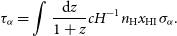
The resulting $\tau_\textrm{eff}$
–
$\tau_\textrm{eff}$
– $\tau_\textrm{eff, GP}$
samples at
$\tau_\textrm{eff, GP}$
samples at $z=5$
are shown in Fig. 2 where
$z=5$
are shown in Fig. 2 where $\tau_\textrm{eff}$
=
$\tau_\textrm{eff}$
= $\tau_\textrm{eff, GP}$
is marked by a diagonal line in each panel. At low values of the neutral fraction, the FGPA tends to overestimate the true value of the effective optical depth. This is especially evident at large overdensities with high values of
$\tau_\textrm{eff, GP}$
is marked by a diagonal line in each panel. At low values of the neutral fraction, the FGPA tends to overestimate the true value of the effective optical depth. This is especially evident at large overdensities with high values of $\tau_\textrm{eff}$
(Kooistra, Lee, & Horowitz Reference Kooistra, Lee and Horowitz2022). As the neutral fraction increases, this bias decreases. However, the scatter in
$\tau_\textrm{eff}$
(Kooistra, Lee, & Horowitz Reference Kooistra, Lee and Horowitz2022). As the neutral fraction increases, this bias decreases. However, the scatter in $p(\tau_\textrm{eff} \ |\ \tau_\textrm{eff, GP}; z, \overline{x}_\textrm{HI})$
increases significantly. At
$p(\tau_\textrm{eff} \ |\ \tau_\textrm{eff, GP}; z, \overline{x}_\textrm{HI})$
increases significantly. At $x_\textrm{HI}\gtrsim0.5$
when damping-wing absorption becomes significant, the FGPA starts to instead underestimate the effective optical depth.
$x_\textrm{HI}\gtrsim0.5$
when damping-wing absorption becomes significant, the FGPA starts to instead underestimate the effective optical depth.
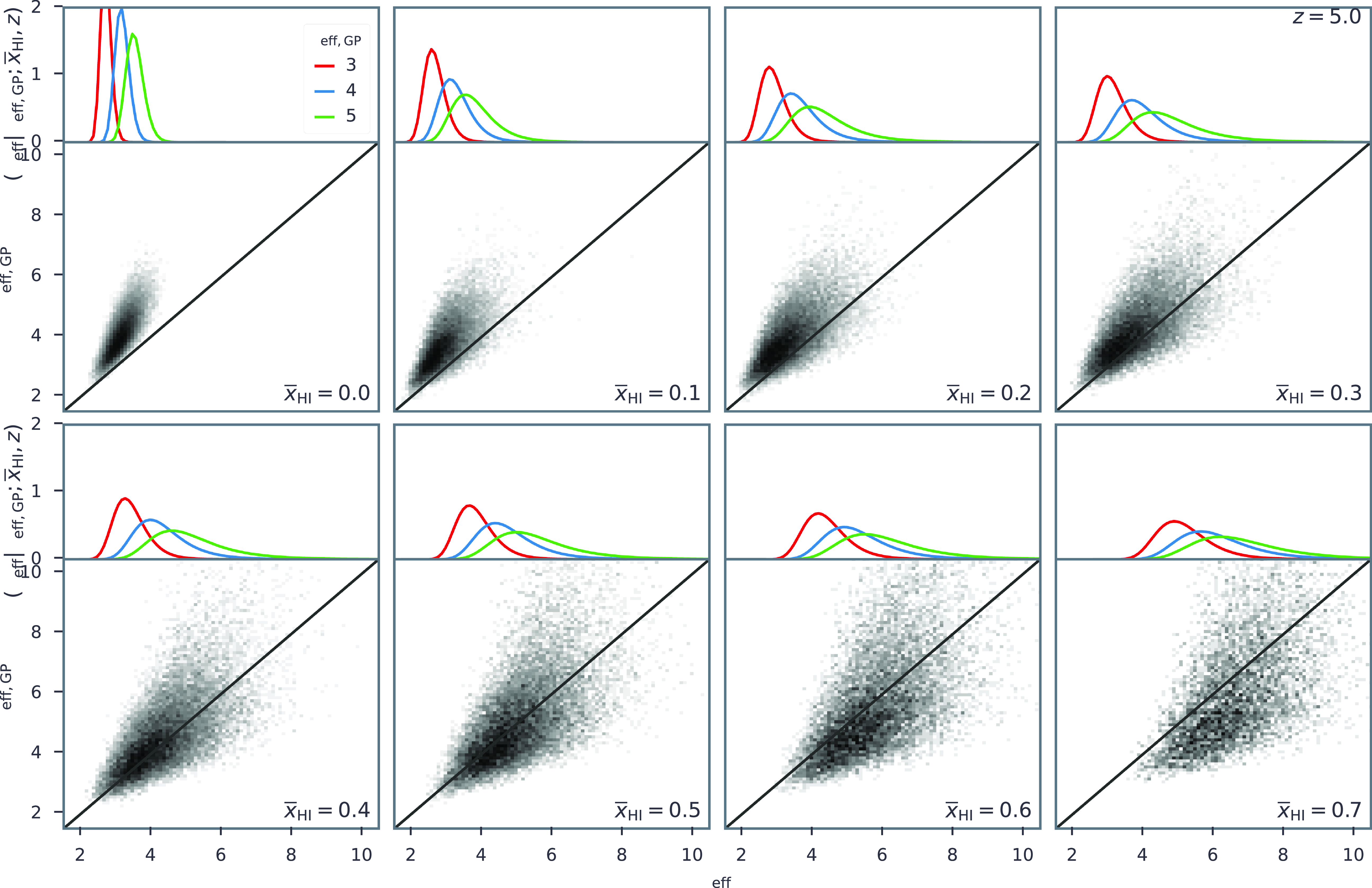
Figure 2.
Lower sub-panels: comparisons of the Ly $\alpha$
effective optical depth calculated using the full integral over the Ly
$\alpha$
effective optical depth calculated using the full integral over the Ly $\alpha$
cross-section at the highest available resolution (
$\alpha$
cross-section at the highest available resolution ( $\tau_\textrm{eff}$
), to those calculated assuming the FGPA (
$\tau_\textrm{eff}$
), to those calculated assuming the FGPA ( $\tau_\textrm{eff, GP}$
). Both calculations use the Sherwood hydrodynamic simulation, with the latter obtained by down-sampling to the same low resolution adopted in our IGM forward-models and ignoring peculiar velocities. These sub-panels show pairs of
$\tau_\textrm{eff, GP}$
). Both calculations use the Sherwood hydrodynamic simulation, with the latter obtained by down-sampling to the same low resolution adopted in our IGM forward-models and ignoring peculiar velocities. These sub-panels show pairs of $\tau_\textrm{eff}$
–
$\tau_\textrm{eff}$
– $\tau_\textrm{eff, GP}$
at different values of the mean neutral fraction,
$\tau_\textrm{eff, GP}$
at different values of the mean neutral fraction, $\overline{x}_\textrm{HI}$
– an incomplete EoR is approximated by randomly placing spherical neutral patches in the simulation box until the desired filling factor of
$\overline{x}_\textrm{HI}$
– an incomplete EoR is approximated by randomly placing spherical neutral patches in the simulation box until the desired filling factor of $\overline{x}_\textrm{HI}$
is reached. These distributions of (
$\overline{x}_\textrm{HI}$
is reached. These distributions of ( $\tau_\textrm{eff}$
,
$\tau_\textrm{eff}$
, $\tau_\textrm{eff, GP}$
) pairs are fit with KDE, resulting in a conditional probability distribution function
$\tau_\textrm{eff, GP}$
) pairs are fit with KDE, resulting in a conditional probability distribution function $p(\tau_\textrm{eff} \ |\ \tau_\textrm{eff, GP}; \overline{x}_\textrm{HI}, z)$
, which is employed to correct our forward-modelled IGM lightcones for missing small scales. Upper sub-panels: example
$p(\tau_\textrm{eff} \ |\ \tau_\textrm{eff, GP}; \overline{x}_\textrm{HI}, z)$
, which is employed to correct our forward-modelled IGM lightcones for missing small scales. Upper sub-panels: example $\tau_\textrm{eff}$
distributions conditioned at
$\tau_\textrm{eff}$
distributions conditioned at $\tau_\textrm{eff, GP}=3$
, 4 and 5.
$\tau_\textrm{eff, GP}=3$
, 4 and 5.
We fit these samples with kernel density estimators (KDEs) in order to obtain an analytic form for $p(\tau_\textrm{eff} \ |\ \tau_\textrm{eff, GP}; z, \overline{x}_\textrm{HI})$
that can be evaluated when forward modelling (c.f. Fig. 1). Specifically, we use 2D conditional Gaussian distributions from the conditional_kde
Footnote
d
package to fit the samples of
$p(\tau_\textrm{eff} \ |\ \tau_\textrm{eff, GP}; z, \overline{x}_\textrm{HI})$
that can be evaluated when forward modelling (c.f. Fig. 1). Specifically, we use 2D conditional Gaussian distributions from the conditional_kde
Footnote
d
package to fit the samples of $1/\tau_\textrm{eff}$
–
$1/\tau_\textrm{eff}$
– $1/\tau_\textrm{eff, GP}$
(as the reciprocal of the optical depth more closely follows a Gaussian distribution). The parameters of the Gaussian kernels (means and standard deviations) are explicit functions of redshift and the neutral fraction,Footnote
e
allowing us to easily evaluate
$1/\tau_\textrm{eff, GP}$
(as the reciprocal of the optical depth more closely follows a Gaussian distribution). The parameters of the Gaussian kernels (means and standard deviations) are explicit functions of redshift and the neutral fraction,Footnote
e
allowing us to easily evaluate $p(\tau_\textrm{eff} \ |\ \tau_\textrm{eff, GP}; z, \overline{x}_\textrm{HI})$
at any neutral fraction and redshift. We show some examples of the fitted conditional distributions in the upper sub-panels of Fig. 2.
$p(\tau_\textrm{eff} \ |\ \tau_\textrm{eff, GP}; z, \overline{x}_\textrm{HI})$
at any neutral fraction and redshift. We show some examples of the fitted conditional distributions in the upper sub-panels of Fig. 2.
3.4 Computing the forest likelihood
For each $\tau_\textrm{eff, GP}(\overline{x}_\textrm{HI}, z)$
calculated using equation (8) on our IGM lightcones, we obtain a random sample from the conditional distributions discussed in the previous subsection:
$\tau_\textrm{eff, GP}(\overline{x}_\textrm{HI}, z)$
calculated using equation (8) on our IGM lightcones, we obtain a random sample from the conditional distributions discussed in the previous subsection: $\tau_\textrm{eff} \sim p(\tau_\textrm{eff} \ |\ \tau_\textrm{eff, GP}; z, \overline{x}_\textrm{HI})$
. Therefore, this leads to a set of effective optical depths that are stochastically corrected for missing sub-structure in the FGPA method. We additionally account for uncertainty in the continuum reconstruction by adding
$\tau_\textrm{eff} \sim p(\tau_\textrm{eff} \ |\ \tau_\textrm{eff, GP}; z, \overline{x}_\textrm{HI})$
. Therefore, this leads to a set of effective optical depths that are stochastically corrected for missing sub-structure in the FGPA method. We additionally account for uncertainty in the continuum reconstruction by adding $\ln(\mathcal{R})$
to every
$\ln(\mathcal{R})$
to every $\tau_\textrm{eff}$
sample. Here,
$\tau_\textrm{eff}$
sample. Here, $\mathcal{R}$
is a random number following a normal distribution centred at unity with a standard deviation of 10%, typical of the continuum reconstruction relative errors (Bosman et al. Reference Bosman2022). Note that we do not account for wavelength correlations in the reconstruction errors or the actual ‘usable’ range of observed wavelengths in each quasar spectrum (see more in Bosman et al. Reference Bosman2022); we plan on including these in future work. We fit the resulting histograms of
$\mathcal{R}$
is a random number following a normal distribution centred at unity with a standard deviation of 10%, typical of the continuum reconstruction relative errors (Bosman et al. Reference Bosman2022). Note that we do not account for wavelength correlations in the reconstruction errors or the actual ‘usable’ range of observed wavelengths in each quasar spectrum (see more in Bosman et al. Reference Bosman2022); we plan on including these in future work. We fit the resulting histograms of $\tau_\textrm{eff}$
in each of the redshift bins defined by the data to obtain the PDFs,
$\tau_\textrm{eff}$
in each of the redshift bins defined by the data to obtain the PDFs, $p(\tau_\textrm{eff}; z)$
.
$p(\tau_\textrm{eff}; z)$
.
These PDFs are our theoretical expectation of the real Universe, for a given model and choice of astrophysical parameters. Therefore, each observed value of $\tau_\textrm{eff}^i$
at
$\tau_\textrm{eff}^i$
at $z^i$
corresponds to a sample from the theoretical PDF, with a corresponding likelihood
$z^i$
corresponds to a sample from the theoretical PDF, with a corresponding likelihood $p(\tau_\textrm{eff} = \tau_\textrm{eff}^i ; z=z^i)$
. For non-detections, we take
$p(\tau_\textrm{eff} = \tau_\textrm{eff}^i ; z=z^i)$
. For non-detections, we take $\tau_\textrm{eff}^i$
to be the 2
$\tau_\textrm{eff}^i$
to be the 2 $\sigma$
lower limit implied by the noise (Bosman et al. Reference Bosman2022).
$\sigma$
lower limit implied by the noise (Bosman et al. Reference Bosman2022).
It is worth noting that the likelihood distribution, $p(\tau_\textrm{eff},z)$
, is forward-modeled, meaning it is sampled by running the simulator many times, varying the most relevant sources of stochasticity together with the astrophysical parameters. This is known as an implicit likelihood, as it avoids the need to specify an explicit likelihood function such as a Gaussian, when comparing data to model. Instead, the simulator itself generates data realisations allowing the observed data to be treated as a sample of this data distribution, for the correct astrophysical parameters. This makes it particularly powerful for cases where the likelihood is too complex or intractable to express analytically (Cranmer, Brehmer, & Louppe Reference Cranmer, Brehmer and Louppe2020; Davies et al. Reference Davies2024). Indeed, inferences using an implicit likelihood (also called simulation-based inference) are becoming increasingly popular in this field (e.g. Zhao, Mao, & Wandelt Reference Zhao, Mao and Wandelt2022; Prelogović & Mesinger 2023; Davies et al. Reference Davies2024; Greig et al. Reference Greig2024,?) as most EoR datasets do not have an analytically-tractable likelihood; and common assumptions of Gaussian pseudo-likelihoods can result in biased posteriors (see Prelogović & Mesinger 2023).
$p(\tau_\textrm{eff},z)$
, is forward-modeled, meaning it is sampled by running the simulator many times, varying the most relevant sources of stochasticity together with the astrophysical parameters. This is known as an implicit likelihood, as it avoids the need to specify an explicit likelihood function such as a Gaussian, when comparing data to model. Instead, the simulator itself generates data realisations allowing the observed data to be treated as a sample of this data distribution, for the correct astrophysical parameters. This makes it particularly powerful for cases where the likelihood is too complex or intractable to express analytically (Cranmer, Brehmer, & Louppe Reference Cranmer, Brehmer and Louppe2020; Davies et al. Reference Davies2024). Indeed, inferences using an implicit likelihood (also called simulation-based inference) are becoming increasingly popular in this field (e.g. Zhao, Mao, & Wandelt Reference Zhao, Mao and Wandelt2022; Prelogović & Mesinger 2023; Davies et al. Reference Davies2024; Greig et al. Reference Greig2024,?) as most EoR datasets do not have an analytically-tractable likelihood; and common assumptions of Gaussian pseudo-likelihoods can result in biased posteriors (see Prelogović & Mesinger 2023).
We obtain the final forest likelihood by multiplying the implicit likelihoods over all XQR-30+ quasars, i, and over all redshift bins used in the analysis. Specifically, we take $\mathcal{L}_\textrm{forest}=\prod_{z=5.3}^{z=6.1} \prod_{i} p(\tau_\textrm{eff} = \tau_\textrm{eff}^i ; z)$
. We do not include data at
$\mathcal{L}_\textrm{forest}=\prod_{z=5.3}^{z=6.1} \prod_{i} p(\tau_\textrm{eff} = \tau_\textrm{eff}^i ; z)$
. We do not include data at $z\leq5.2$
in order to make our likelihood more sensitive to the EoR (see e.g. Bosman et al. Reference Bosman2022 who showed that the EoR ends sometime before
$z\leq5.2$
in order to make our likelihood more sensitive to the EoR (see e.g. Bosman et al. Reference Bosman2022 who showed that the EoR ends sometime before $z\sim5.2$
).
$z\sim5.2$
).
Note that this procedure does not account for higher order correlations in the mapping from $\tau_\textrm{eff, GP}$
to
$\tau_\textrm{eff, GP}$
to $\tau_\textrm{eff}$
. Moreover, it assumes that each
$\tau_\textrm{eff}$
. Moreover, it assumes that each $\Delta z$
= 0.1 (
$\Delta z$
= 0.1 ( $\sim$
40 cMpc) segment is an independent sample of
$\sim$
40 cMpc) segment is an independent sample of $p(\tau_\textrm{eff}; z)$
; i.e. we ignore the covariance between the
$p(\tau_\textrm{eff}; z)$
; i.e. we ignore the covariance between the $\Delta z$
= 0.1 segments extracted from a single quasar spectrum. We expect the covariance on such large scales to have only a minor impact on the total likelihood. Nevertheless, we plan on relaxing this approximation in future work in which we will use simulation-based inference for the total likelihood, accounting for large scale correlations in both the effective optical depths and reconstruction errors.
$\Delta z$
= 0.1 segments extracted from a single quasar spectrum. We expect the covariance on such large scales to have only a minor impact on the total likelihood. Nevertheless, we plan on relaxing this approximation in future work in which we will use simulation-based inference for the total likelihood, accounting for large scale correlations in both the effective optical depths and reconstruction errors.
3.5 Combining with complementary observations
We also account for complementary, independent data when performing inference. Specifically, we compute additional likelihood terms for: (i) the galaxy non-ionising UV LFs well-established by Hubble at $6\leq z \leq 10$
(Bouwens et al. Reference Bouwens2015b, Reference Bouwens2016; Oesch et al. Reference Oesch, Bouwens, Illingworth, Labbé and Stefanon2018); and (ii) the CMB polarisation power spectra observed by Planck (Planck Collaboration et al. Reference Collaboration2020). These two datasets are independent and mature, and can therefore be interpreted robustly. Unlike Q21, we do not include a likelihood term for the pixel Dark Fraction (Mesinger Reference Mesinger2010; McGreer, Mesinger, & D’Odorico Reference McGreer, Mesinger and D’Odorico2015) as this statistic is also based on Lyman forests and therefore is technically not fully independent from the optical depth distributions discussed above. Thus our total likelihood consists of the product of three terms:
$6\leq z \leq 10$
(Bouwens et al. Reference Bouwens2015b, Reference Bouwens2016; Oesch et al. Reference Oesch, Bouwens, Illingworth, Labbé and Stefanon2018); and (ii) the CMB polarisation power spectra observed by Planck (Planck Collaboration et al. Reference Collaboration2020). These two datasets are independent and mature, and can therefore be interpreted robustly. Unlike Q21, we do not include a likelihood term for the pixel Dark Fraction (Mesinger Reference Mesinger2010; McGreer, Mesinger, & D’Odorico Reference McGreer, Mesinger and D’Odorico2015) as this statistic is also based on Lyman forests and therefore is technically not fully independent from the optical depth distributions discussed above. Thus our total likelihood consists of the product of three terms: $\mathcal{L}_\textrm{tot}\ =\ \mathcal{L}_\textrm{forest } \times \mathcal{L}_\textrm{LF} \times \mathcal{L}_\textrm{CMB}$
, where the final two correspond to the LF and CMB likelihoods, discussed further below.
$\mathcal{L}_\textrm{tot}\ =\ \mathcal{L}_\textrm{forest } \times \mathcal{L}_\textrm{LF} \times \mathcal{L}_\textrm{CMB}$
, where the final two correspond to the LF and CMB likelihoods, discussed further below.
We construct the UV LF likelihood following Park et al. (Reference Park, Mesinger, Greig and Gillet2019). Specifically, we assume a Gaussian likelihood in each magnitude bin, $M_\textrm{UV,i}$
, with a negligible covariance between bins (see e.g. Leethochawalit et al. Reference Leethochawalit, Roberts-Borsani, Morishita, Trenti and Treu2023 for an alternative approach). The UV LF likelihood is thus
$M_\textrm{UV,i}$
, with a negligible covariance between bins (see e.g. Leethochawalit et al. Reference Leethochawalit, Roberts-Borsani, Morishita, Trenti and Treu2023 for an alternative approach). The UV LF likelihood is thus $\mathcal{L}_\textrm{LF,tot}=\prod_{z=6}^{z=10} \prod_{i} \exp\left\{-\left[{\Delta \phi(M_\textrm{UV},i)}/{\sigma_\phi(M_\textrm{UV},i)}\right]^2\right\}$
, where
$\mathcal{L}_\textrm{LF,tot}=\prod_{z=6}^{z=10} \prod_{i} \exp\left\{-\left[{\Delta \phi(M_\textrm{UV},i)}/{\sigma_\phi(M_\textrm{UV},i)}\right]^2\right\}$
, where $\Delta \phi$
is the difference between forward-modelled and observed galaxy number densities in a given magnitude and redshift bin, and the corresponding observational uncertainties are
$\Delta \phi$
is the difference between forward-modelled and observed galaxy number densities in a given magnitude and redshift bin, and the corresponding observational uncertainties are $\sigma_\phi$
. As dust is thought to significantly suppress the UV LFs in the bright end (Mason, Trenti, & Treu Reference Mason, Trenti and Treu2023; Qin, Balu, & Wyithe Reference Qin, Balu and Wyithe2023), we only consider magnitudes fainter than
$\sigma_\phi$
. As dust is thought to significantly suppress the UV LFs in the bright end (Mason, Trenti, & Treu Reference Mason, Trenti and Treu2023; Qin, Balu, & Wyithe Reference Qin, Balu and Wyithe2023), we only consider magnitudes fainter than $M_\textrm{UV}=-20$
to avoid modelling dust attenuation, and use the redshift range between
$M_\textrm{UV}=-20$
to avoid modelling dust attenuation, and use the redshift range between $z=6$
and 10 spanning the EoR.
$z=6$
and 10 spanning the EoR.
We construct the Planck CMB likelihood as a two-sided Gaussian on the Thomson scattering optical depth summary statistic inferred by Qin et al. (Reference Qin, Poulin, Mesinger, Greig, Murray and Park2020): $\tau_e=0.0569^{+0.0073}_{-0.0066}$
. Specifically, we take the form
$\tau_e=0.0569^{+0.0073}_{-0.0066}$
. Specifically, we take the form $\mathcal{L}_\textrm{CMB} = \exp\left[\def\negativespace{}-\left({\Delta \tau_e}/{\sigma_{\tau_e}}\right)^2\right]$
, where
$\mathcal{L}_\textrm{CMB} = \exp\left[\def\negativespace{}-\left({\Delta \tau_e}/{\sigma_{\tau_e}}\right)^2\right]$
, where $\Delta \tau_e$
represents the difference between the forward-modelled and measured optical depths while
$\Delta \tau_e$
represents the difference between the forward-modelled and measured optical depths while $\sigma_{\tau_e}$
is the observational uncertainty. Note that Qin et al. (Reference Qin, Poulin, Mesinger, Greig, Murray and Park2020) found very little difference in the inferred posteriors when using a likelihood defined directly on the E-mode polarisation power spectra compared to using a Gaussian likelihood on the
$\sigma_{\tau_e}$
is the observational uncertainty. Note that Qin et al. (Reference Qin, Poulin, Mesinger, Greig, Murray and Park2020) found very little difference in the inferred posteriors when using a likelihood defined directly on the E-mode polarisation power spectra compared to using a Gaussian likelihood on the $\tau_e$
summary derived from the power spectra. We thus use the latter as it is much more computationally efficient.
$\tau_e$
summary derived from the power spectra. We thus use the latter as it is much more computationally efficient.
Figure 3. Inferred $\tau_\textrm{eff}$
CDFs from our fiducial model from
$\tau_\textrm{eff}$
CDFs from our fiducial model from $z=$
5.3 to 6.1. To account for cosmic variance, we randomly select from each model in the posterior the same number of sightlines as in the XQR-30+ observational dataset. The red regions indicate the 95% C.I. For comparison, the XQR-30+ observations are shown in grey with non-detections denoted with the shaded regions spanning the flux range between zero and double the noise (Bosman et al. Reference Bosman2022). A number of theoretical results are shown for comparison (Kulkarni et al. Reference Kulkarni, Keating, Haehnelt, Bosman, Puchwein, Chardin and Aubert2019; Garaldi et al. Reference Garaldi, Kannan, Smith, Springel, Pakmor, Vogelsberger and Hernquist2022; Cain et al. Reference Cain, D’Aloisio, Lopez, Gangolli and Roth2024; Davies et al. Reference Davies2024, optimistic; with earlier works using slightly different binning for
$z=$
5.3 to 6.1. To account for cosmic variance, we randomly select from each model in the posterior the same number of sightlines as in the XQR-30+ observational dataset. The red regions indicate the 95% C.I. For comparison, the XQR-30+ observations are shown in grey with non-detections denoted with the shaded regions spanning the flux range between zero and double the noise (Bosman et al. Reference Bosman2022). A number of theoretical results are shown for comparison (Kulkarni et al. Reference Kulkarni, Keating, Haehnelt, Bosman, Puchwein, Chardin and Aubert2019; Garaldi et al. Reference Garaldi, Kannan, Smith, Springel, Pakmor, Vogelsberger and Hernquist2022; Cain et al. Reference Cain, D’Aloisio, Lopez, Gangolli and Roth2024; Davies et al. Reference Davies2024, optimistic; with earlier works using slightly different binning for $\tau_\textrm{eff}$
).
$\tau_\textrm{eff}$
).
3.6 Summary of model parameters and associated priors
Before showing our inference results, we summarise the free parameters used in our galaxy models and their associated prior ranges (see also Table 1).
-
1.
$\log_{10}f_{*,10}\in[\def\negativespace{}-2,-0.5]$
: the fraction of galactic baryons in stars, normalised at
$M_\textrm{vir}=10^{10}\,{\rm M}_\odot$
. This parameter sets the normalisation of the stellar-to-halo mass relation, and its prior range is motivated by observations and simulations of high-redshift galaxies (Dayal et al. Reference Dayal, Ferrara, Dunlop and Pacucci2014; Mutch et al. Reference Mutch, Geil, Poole, Angel, Duffy, Mesinger and Wyithe2016; Behroozi et al. Reference Behroozi, Wechsler, Hearin and Conroy2019; Bird et al. Reference Bird, Ni, Di Matteo, Croft, Feng and Chen2022; Stefanon et al. Reference Stefanon, Bouwens, Labbé, Illingworth, Gonzalez and Oesch2021). -
2.
$\alpha_*\in[0, 1.0]$
: the power law index relating the stellar fraction to the halo mass. This parameter determines the slope of the stellar-to-halo mass relation. Observations of the faint end of the UV LFs suggest more efficient star formation in more massive galaxies (Bouwens et al. Reference Bouwens2015b; Oesch et al. Reference Oesch, Bouwens, Illingworth, Labbé and Stefanon2018), motivating our prior range. -
3.
$\log_{10}f_\textrm{esc,10}\in[\def\negativespace{}-3,0]$
: the amplitude of the power-law relating the UV ionising escape fraction to halo mass, normalised at
$M_\textrm{vir}=10^{10}\,{\rm M}_\odot$
. The wide prior reflects the large uncertainties in both low-redshift observations (Vanzella et al. Reference Vanzella2010, Reference Vanzella2016; Boutsia et al. Reference Boutsia2011; Nestor et al. Reference Nestor, Shapley, Kornei, Steidel and Siana2013; Guaita et al. Reference Guaita2016; Grazian et al. Reference Grazian2016; Shapley et al. Reference Shapley, Steidel and Strom2016; Bian et al. Reference Bian, Fan, McGreer, Cai and Jiang2017; Steidel et al. Reference Steidel2018; Naidu et al. Reference Naidu, Forrest, Oesch, Tran and Holden2018; Fletcher et al. Reference Fletcher, Tang, Robertson, Nakajima, Ellis, Stark and Inoue2019; Izotov et al. Reference Izotov, Worseck, Schaerer, Guseva, Chisholm, Thuan, Fricke and Verhamme2021; Pahl et al. Reference Pahl, Shapley, Steidel, Chen and Reddy2021) and reionisation simulations (Kostyuk et al. Reference Kostyuk, Nelson, Ciardi, Glatzle and Pillepich2023; Choustikov et al. Reference Choustikov2024; Mutch et al. Reference Mutch, Greig, Qin, Poole and Wyithe2024). -
4.
$\alpha_\textrm{esc}\in[\def\negativespace{}-1, 0.5]$
: the power law slope of the UV ionising escape fraction to halo mass relation. Galaxy simulations seem to suggest boosted Lyman continuum leakage in less massive galaxies as supernovae evacuate low column density channels from shallow gravitational potentials (Paardekooper, Khochfar, & Dalla Vecchia Reference Paardekooper, Khochfar and Dalla Vecchia2015; Xu et al. Reference Xu, Wise, Norman, Ahn and O’Shea2016; Kostyuk et al. Reference Kostyuk, Nelson, Ciardi, Glatzle and Pillepich2023; Mutch et al. Reference Mutch, Greig, Qin, Poole and Wyithe2024). This motivates a wider negative range in the prior, although we caution that this is highly uncertain and therefore still allow positive values in our prior (e.g. Ma et al. Reference Ma, Kasen, Hopkins, Faucher-Giguère, Quataert, Kereš and Murray2015; Naidu et al. Reference Naidu, Tacchella, Mason, Bose, Oesch and Conroy2020; Rosdahl et al. Reference Rosdahl2022; Bhagwat et al. Reference Bhagwat, Costa, Ciardi, Pakmor and Garaldi2024). -
5.
$\beta_\textrm{esc}\in[\def\negativespace{}-3, 3]$
: the power law scaling index of the UV ionising escape fraction as a function of redshift, used only in
$\texttt{Evolving_f}_\texttt{esc}$
. The prior is somewhat arbitrary with the upper and lower limits allowing
$f_\textrm{esc}$
to scale similarly.Footnote
f
-
6.
$\tau_\ast\in(0, 1]$
: the star formation timescale in units of the Hubble time. The flat prior encompasses extreme cases where the entire stellar mass is formed in an instantaneous burst event or gradually built over the age of the universe. -
7.
$\log_{10}(M_\textrm{turn}/\mathrm{M_\odot})\in[8, 10]$
: the characteristic halo mass below which star formation becomes exponentially suppressed. The lower and upper limits of the flat prior are motivated by the atomic cooling threshold and the faintest, currently observed high-redshift galaxies (e.g. Bouwens et al. Reference Bouwens2016, Reference Bouwens2015b; Oesch et al. Reference Oesch, Bouwens, Illingworth, Labbé and Stefanon2018), respectively.


4. Fiducial inference results
As can be seen from Table 1, the Bayesian evidence ratios suggest that the data have a very strong preference (Jeffreys Reference Jeffreys1939) for the $\texttt{Evolving_f}_\texttt{esc}$
model. We therefore treat this model as ‘fiducial’, presenting its posterior in this section, before comparing it to the
$\texttt{Evolving_f}_\texttt{esc}$
model. We therefore treat this model as ‘fiducial’, presenting its posterior in this section, before comparing it to the $\texttt{Constant_f}_\texttt{esc}$
model in the following section.Footnote
g
Alternatively, one could do Bayesian model averaging to combine the derived IGM and galaxy properties from different models; however the evidence ratio in this case is so strongly skewed towards
$\texttt{Constant_f}_\texttt{esc}$
model in the following section.Footnote
g
Alternatively, one could do Bayesian model averaging to combine the derived IGM and galaxy properties from different models; however the evidence ratio in this case is so strongly skewed towards $\texttt{Evolving_f}_\texttt{esc}$
, that the model-averaged posteriors would just follow the
$\texttt{Evolving_f}_\texttt{esc}$
, that the model-averaged posteriors would just follow the $\texttt{Evolving_f}_\texttt{esc}$
ones.
$\texttt{Evolving_f}_\texttt{esc}$
ones.
We show the posteriors in the space of galaxy parameters in Appendix A. Here we focus on the inferred IGM properties and galaxy scaling relations.
4.1 Effective optical depth distributions
In Fig. 3, we plot the recovered optical depth CDFs in red enclosing the 95% confidence interval (C.I.). Observational data from Bosman et al. (Reference Bosman2022) are shown in grey. The red-shaded regions are constructed from the posterior samples, each having the same number of randomly selected sightlines per redshift bin as in the data to account for cosmic variance. We note that the cosmic variance dominates the widths of the CDFs, especially at the highest redshifts.
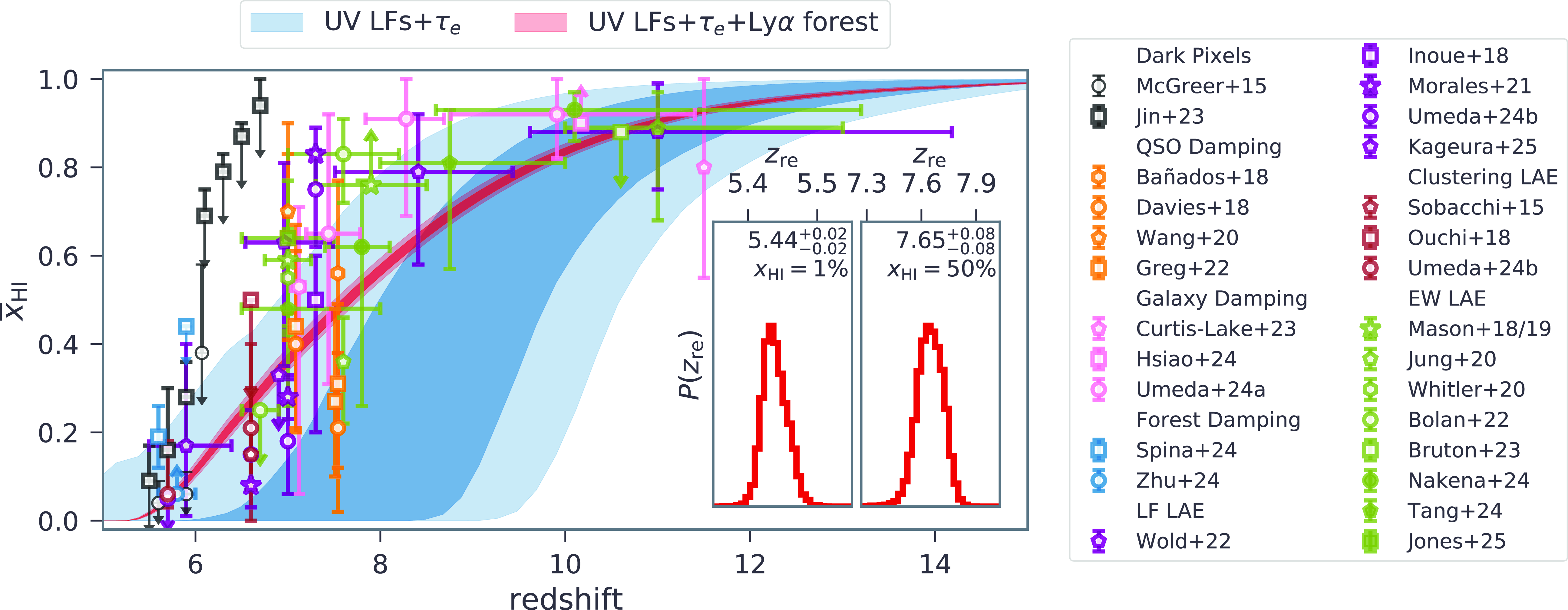
Figure 4. The inferred EoR history using our fiducial model. The blue-shaded region uses only UV LFs and CMB $\tau_e$
data (a likelihood of
$\tau_e$
data (a likelihood of $\mathcal{L}_\textrm{LF} \times \mathcal{L}_\textrm{CMB}$
), while the red additionally includes the Ly
$\mathcal{L}_\textrm{LF} \times \mathcal{L}_\textrm{CMB}$
), while the red additionally includes the Ly $\alpha$
forest
$\alpha$
forest $\tau_\textrm{eff}$
distributions (likelihood of
$\tau_\textrm{eff}$
distributions (likelihood of $\mathcal{L}_\textrm{forest } \times \mathcal{L}_\textrm{LF} \times \mathcal{L}_\textrm{CMB}$
). In both cases, the dark (light) regions indicate the 68% and 95% C.I. The XQR-30+ forest data are very constraining; including them makes the posterior transition from being prior-dominated to being likelihood-dominated. PDFs of the redshifts corresponding to
$\mathcal{L}_\textrm{forest } \times \mathcal{L}_\textrm{LF} \times \mathcal{L}_\textrm{CMB}$
). In both cases, the dark (light) regions indicate the 68% and 95% C.I. The XQR-30+ forest data are very constraining; including them makes the posterior transition from being prior-dominated to being likelihood-dominated. PDFs of the redshifts corresponding to $\overline{x}_\textrm{HI}=$
0.01 and 0.5 are presented in the inset panels, showing that in our fiducial model reionisation ends at
$\overline{x}_\textrm{HI}=$
0.01 and 0.5 are presented in the inset panels, showing that in our fiducial model reionisation ends at $z=5.44\pm0.02$
and the EoR mid-point is at
$z=5.44\pm0.02$
and the EoR mid-point is at $z=7.7\pm0.1$
. Estimates of the ionisation state of the universe coming from other probes are also shown for illustrative purposes including the dark pixel upper limits (McGreer, Mesinger, & D’Odorico Reference McGreer, Mesinger and D’Odorico2015; Jin et al. Reference Jin2023), Lyman-α damping-wing absorption in QSOs (Eduardo Bañados et al. Reference Bañados2018; Davies et al. Reference Davies2018; Wang et al. Reference Wang2020; Greig et al. Reference Greig, Mesinger, Davies, Wang, Yang and Hennawi2022; see also Mesinger & Haiman Reference Mesinger and Haiman2004; Greig et al. Reference Greig, Mesinger, Haiman and Simcoe2017; Greig, Mesinger, & Bañados Reference Greig, Mesinger and Bañados2019), in galaxies (Curtis-Lake et al. Reference Curtis-Lake2023; Hsiao et al. Reference Hsiao2024; Umeda et al. Reference Umeda, Ouchi, Nakajima, Harikane, Ono, Xu, Isobe and Zhang2024), or in forests (Spina et al. Reference Spina, Bosman, Davies, Gaikwad and Zhu2024; Zhu et al. Reference Zhu2024), Lyman-α equivalent widths (Mason et al. Reference Mason2019; Jung et al. Reference Jung2020; Whitler et al. Reference Whitler, Mason, Ren, Dijkstra, Mesinger, Pentericci, Trenti and Treu2020; Bolan et al. Reference Bolan2022; Bruton et al. Reference Bruton, Lin, Scarlata and Hayes2023; Nakane et al. Reference Nakane2024; Tang et al. Reference Tang, Stark, Topping, Mason and Ellis2024; Jones et al. Reference Jones2025; see also Mesinger et al. Reference Mesinger, Aykutalp, Vanzella, Pentericci, Ferrara and Dijkstra2015), and the LF (Inoue et al. Reference Inoue2018; Morales et al. Reference Morales, Mason, Bruton, Gronke, Haardt and Scarlata2021; Wold et al. Reference Wold2022; Umeda et al. Reference Umeda, Ouchi, Nakajima, Harikane, Ono, Xu, Isobe and Zhang2024; Kageura et al. Reference Kageura2025) or clustering of Lyα emitters (Sobacchi & Mesinger Reference Sobacchi and Mesinger2015; Ouchi et al. Reference Ouchi2018; Umeda et al. Reference Umeda, Ouchi, Nakajima, Harikane, Ono, Xu, Isobe and Zhang2024), most of which are consistent with our results despite not being included in the inference.
$z=7.7\pm0.1$
. Estimates of the ionisation state of the universe coming from other probes are also shown for illustrative purposes including the dark pixel upper limits (McGreer, Mesinger, & D’Odorico Reference McGreer, Mesinger and D’Odorico2015; Jin et al. Reference Jin2023), Lyman-α damping-wing absorption in QSOs (Eduardo Bañados et al. Reference Bañados2018; Davies et al. Reference Davies2018; Wang et al. Reference Wang2020; Greig et al. Reference Greig, Mesinger, Davies, Wang, Yang and Hennawi2022; see also Mesinger & Haiman Reference Mesinger and Haiman2004; Greig et al. Reference Greig, Mesinger, Haiman and Simcoe2017; Greig, Mesinger, & Bañados Reference Greig, Mesinger and Bañados2019), in galaxies (Curtis-Lake et al. Reference Curtis-Lake2023; Hsiao et al. Reference Hsiao2024; Umeda et al. Reference Umeda, Ouchi, Nakajima, Harikane, Ono, Xu, Isobe and Zhang2024), or in forests (Spina et al. Reference Spina, Bosman, Davies, Gaikwad and Zhu2024; Zhu et al. Reference Zhu2024), Lyman-α equivalent widths (Mason et al. Reference Mason2019; Jung et al. Reference Jung2020; Whitler et al. Reference Whitler, Mason, Ren, Dijkstra, Mesinger, Pentericci, Trenti and Treu2020; Bolan et al. Reference Bolan2022; Bruton et al. Reference Bruton, Lin, Scarlata and Hayes2023; Nakane et al. Reference Nakane2024; Tang et al. Reference Tang, Stark, Topping, Mason and Ellis2024; Jones et al. Reference Jones2025; see also Mesinger et al. Reference Mesinger, Aykutalp, Vanzella, Pentericci, Ferrara and Dijkstra2015), and the LF (Inoue et al. Reference Inoue2018; Morales et al. Reference Morales, Mason, Bruton, Gronke, Haardt and Scarlata2021; Wold et al. Reference Wold2022; Umeda et al. Reference Umeda, Ouchi, Nakajima, Harikane, Ono, Xu, Isobe and Zhang2024; Kageura et al. Reference Kageura2025) or clustering of Lyα emitters (Sobacchi & Mesinger Reference Sobacchi and Mesinger2015; Ouchi et al. Reference Ouchi2018; Umeda et al. Reference Umeda, Ouchi, Nakajima, Harikane, Ono, Xu, Isobe and Zhang2024), most of which are consistent with our results despite not being included in the inference.
We see from the figure that our fiducial model excels at recovering the observed $\tau_\textrm{eff}$
CDFs throughout this redshift range – despite individual
$\tau_\textrm{eff}$
CDFs throughout this redshift range – despite individual $\tau_\textrm{eff}$
data being used in the likelihood, our model can recover both the mean and the shape of the observed optical depth distribution. We stress that most previous work either used hyperparameters to account for the mean opacity evolution (e.g., Q21), calibrated the models to have the same mean opacity as the data and/or treated each redshift bin independently (e.g. Kulkarni et al. Reference Kulkarni, Keating, Haehnelt, Bosman, Puchwein, Chardin and Aubert2019; Meiksin Reference Meiksin2020; Cain et al. Reference Cain, D’Aloisio, Lopez, Gangolli and Roth2024; Gaikwad et al. Reference Gaikwad2023;Footnote
h
Davies et al. Reference Davies2024). Some more expensive coupled hydrodynamic and radiative-transfer simulations such as CODA and THESAN (Ocvirk et al. Reference Ocvirk, Lewis, Gillet, Chardin, Aubert, Deparis and Thélie2021; Garaldi et al. Reference Garaldi, Kannan, Smith, Springel, Pakmor, Vogelsberger and Hernquist2022) do not directly tune their simulations to reproduce the forest data; however their predicted CDFs do not agree with the data as well as most of the other previously mentioned works. For illustration, we show some of these results in Fig. 3.
$\tau_\textrm{eff}$
data being used in the likelihood, our model can recover both the mean and the shape of the observed optical depth distribution. We stress that most previous work either used hyperparameters to account for the mean opacity evolution (e.g., Q21), calibrated the models to have the same mean opacity as the data and/or treated each redshift bin independently (e.g. Kulkarni et al. Reference Kulkarni, Keating, Haehnelt, Bosman, Puchwein, Chardin and Aubert2019; Meiksin Reference Meiksin2020; Cain et al. Reference Cain, D’Aloisio, Lopez, Gangolli and Roth2024; Gaikwad et al. Reference Gaikwad2023;Footnote
h
Davies et al. Reference Davies2024). Some more expensive coupled hydrodynamic and radiative-transfer simulations such as CODA and THESAN (Ocvirk et al. Reference Ocvirk, Lewis, Gillet, Chardin, Aubert, Deparis and Thélie2021; Garaldi et al. Reference Garaldi, Kannan, Smith, Springel, Pakmor, Vogelsberger and Hernquist2022) do not directly tune their simulations to reproduce the forest data; however their predicted CDFs do not agree with the data as well as most of the other previously mentioned works. For illustration, we show some of these results in Fig. 3.
4.2 EoR history
In Fig. 4, we show the main result of this work – the inferred reionisation history in our fiducial model. In blue we show the posterior resulting from using only the $\mathcal{L}_\textrm{LF}$
and
$\mathcal{L}_\textrm{LF}$
and $\mathcal{L}_\textrm{CMB}$
likelihood terms. This roughly corresponds to our previous state of knowledge, without using the forest data.Footnote
i
From the blue region we see that the CMB optical depth and the UV LFs do not result in tight constraints on the EoR history. The UV LFs loosely constrain the evolution of the star formation rate density (SFRD), while the CMB optical depth additionally constrains the corresponding ionising escape fraction (see the parameter posterior shown in blue in Fig. A1). Given that these constraints are not tight, the posterior is prior dominated (as opposed to being likelihood dominated). Since we chose broad priors, allowing the ionising escape fraction to extend to unity, most of the posterior volume traces a relatively early reionisation, with midpoints around
$\mathcal{L}_\textrm{CMB}$
likelihood terms. This roughly corresponds to our previous state of knowledge, without using the forest data.Footnote
i
From the blue region we see that the CMB optical depth and the UV LFs do not result in tight constraints on the EoR history. The UV LFs loosely constrain the evolution of the star formation rate density (SFRD), while the CMB optical depth additionally constrains the corresponding ionising escape fraction (see the parameter posterior shown in blue in Fig. A1). Given that these constraints are not tight, the posterior is prior dominated (as opposed to being likelihood dominated). Since we chose broad priors, allowing the ionising escape fraction to extend to unity, most of the posterior volume traces a relatively early reionisation, with midpoints around $z=8$
–9.
$z=8$
–9.
The red shaded region in the figure shows what happens to the posterior when we further include the Ly $\alpha$
forest data, i.e. with the total likelihood of
$\alpha$
forest data, i.e. with the total likelihood of $\mathcal{L}_\textrm{forest } \times \mathcal{L}_\textrm{LF} \times \mathcal{L}_\textrm{CMB}$
. The EoR history,
$\mathcal{L}_\textrm{forest } \times \mathcal{L}_\textrm{LF} \times \mathcal{L}_\textrm{CMB}$
. The EoR history, $\overline{x}_\textrm{HI}(z)$
, of the maximum-a-posteriori (MAP) model is listed in Table A1, and is well fit by a rational function
$\overline{x}_\textrm{HI}(z)$
, of the maximum-a-posteriori (MAP) model is listed in Table A1, and is well fit by a rational function
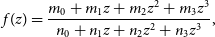 \begin{equation}\begin{split} f(z) = \frac{m_0+m_1z+m_2z^2+m_3z^3}{n_0+n_1z+n_2z^2+n_3z^3},\end{split}\end{equation}
with parameters $\{m_0,m_1,m_2,m_3,n_0,n_1,n_2,n_3\}$
= {292.6, −105.47, 7.824, 0.312, −24.3, 22.9, −4.96, 0.694}. It is obvious that the
$\{m_0,m_1,m_2,m_3,n_0,n_1,n_2,n_3\}$
= {292.6, −105.47, 7.824, 0.312, −24.3, 22.9, −4.96, 0.694}. It is obvious that the $\tau_\textrm{eff}$
data are extremely constraining, resulting in a very narrow posterior. The uncertainties are over an order of magnitude smaller than without the forest data, with most of the history constrained to better than
$\tau_\textrm{eff}$
data are extremely constraining, resulting in a very narrow posterior. The uncertainties are over an order of magnitude smaller than without the forest data, with most of the history constrained to better than $\Delta z \sim 0.1$
at the 68% C.I. The forest data require the EoR to be ongoing below
$\Delta z \sim 0.1$
at the 68% C.I. The forest data require the EoR to be ongoing below $z \leq 6$
(see also the previous results in Choudhury, Paranjape, & Bosman Reference Choudhury, Paranjape and Bosman2021 and Q21). From the inset panels in the figure, we see that in this fiducial model reionisation ends at
$z \leq 6$
(see also the previous results in Choudhury, Paranjape, & Bosman Reference Choudhury, Paranjape and Bosman2021 and Q21). From the inset panels in the figure, we see that in this fiducial model reionisation ends at $z=5.44\pm0.02$
and the EoR mid-point is at
$z=5.44\pm0.02$
and the EoR mid-point is at $z=7.7\pm0.1$
. Consequently, the inferred CMB optical depth is also tightly constrained with
$z=7.7\pm0.1$
. Consequently, the inferred CMB optical depth is also tightly constrained with $\tau_{e}=0.0589\pm 0.001$
(
$\tau_{e}=0.0589\pm 0.001$
( $1\sigma$
) compared to
$1\sigma$
) compared to $\tau_{e}=0.0571\pm 0.006$
when the forest is not included.
$\tau_{e}=0.0571\pm 0.006$
when the forest is not included.
Perhaps surprisingly, the forest data tightly constrain the EoR history at redshifts beyond where we have forest data, $z\gt6.3$
. These constraints are indirect, coming from the combination of HMF evolution, the SFR to halo mass implied by UV LF observations, and the ionising escape fraction scalings required to match the forest. The forest in particular provides a firm anchor for our models. The forest data requires a photon-starved end to reionisation, with recombinations starting to balance ionisations, in order to smoothly transition into the post EoR regime (Bolton & Haehnelt Reference Bolton and Haehnelt2007; Sobacchi & Mesinger Reference Sobacchi and Mesinger2014). Such a ‘soft-landing’ is difficult to achieve with small-box EoR simulations (e.g., Barkana & Loeb Reference Barkana and Loeb2004) and/or with those that cannot resolve recombinations in the late EoR stages (c.f. Fig. 6 in Sobacchi & Mesinger Reference Sobacchi and Mesinger2014, and Qin et al. Reference Qin, Mesinger, Bosman and Viel2021; Cain et al. Reference Cain, D’Aloisio, Lopez, Gangolli and Roth2024). Such limitations tend to result in an overly rapid evolution of the late EoR stages, which in turn requires ad-hoc corrections/tuning (e.g., a very rapid drop in emissivity) in order to match forest data (see Fig. 7 and associated discussion). The fact that our box sizes are 250 Mpc and that sub-grid recombinations are computed analytically (and thus not limited by resolution), likely allows us to capture this ‘soft-landing’ preferred by the forest data. We caution however that these constraints on the EoR history at
$z\gt6.3$
. These constraints are indirect, coming from the combination of HMF evolution, the SFR to halo mass implied by UV LF observations, and the ionising escape fraction scalings required to match the forest. The forest in particular provides a firm anchor for our models. The forest data requires a photon-starved end to reionisation, with recombinations starting to balance ionisations, in order to smoothly transition into the post EoR regime (Bolton & Haehnelt Reference Bolton and Haehnelt2007; Sobacchi & Mesinger Reference Sobacchi and Mesinger2014). Such a ‘soft-landing’ is difficult to achieve with small-box EoR simulations (e.g., Barkana & Loeb Reference Barkana and Loeb2004) and/or with those that cannot resolve recombinations in the late EoR stages (c.f. Fig. 6 in Sobacchi & Mesinger Reference Sobacchi and Mesinger2014, and Qin et al. Reference Qin, Mesinger, Bosman and Viel2021; Cain et al. Reference Cain, D’Aloisio, Lopez, Gangolli and Roth2024). Such limitations tend to result in an overly rapid evolution of the late EoR stages, which in turn requires ad-hoc corrections/tuning (e.g., a very rapid drop in emissivity) in order to match forest data (see Fig. 7 and associated discussion). The fact that our box sizes are 250 Mpc and that sub-grid recombinations are computed analytically (and thus not limited by resolution), likely allows us to capture this ‘soft-landing’ preferred by the forest data. We caution however that these constraints on the EoR history at $z\gt6.3$
are indirect, and as such become increasingly model-dependent at increasingly higher redshifts. We will revisit this in the future using alternate galaxy models that evaluate star-forming duty cycles based on cooling efficiencies and feedback, and include an additional population of early, molecular-cooling galaxies, which might dominate the ionising background at
$z\gt6.3$
are indirect, and as such become increasingly model-dependent at increasingly higher redshifts. We will revisit this in the future using alternate galaxy models that evaluate star-forming duty cycles based on cooling efficiencies and feedback, and include an additional population of early, molecular-cooling galaxies, which might dominate the ionising background at $z\gt10$
–15 (e.g., Qin et al. Reference Qin, Poulin, Mesinger, Greig, Murray and Park2020; Muñoz et al. Reference Muñoz, Qin, Mesinger, Murray, Greig and Mason2022; Ventura et al. Reference Ventura, Qin, Balu and Wyithe2024).
$z\gt10$
–15 (e.g., Qin et al. Reference Qin, Poulin, Mesinger, Greig, Murray and Park2020; Muñoz et al. Reference Muñoz, Qin, Mesinger, Murray, Greig and Mason2022; Ventura et al. Reference Ventura, Qin, Balu and Wyithe2024).
For illustration, we also plot various independent estimates of the IGM neutral fraction using other probes:
-
1. Our results are consistent with upper limits from the dark pixel fraction, applied to smaller forest samples (McGreer, Mesinger, & D’Odorico Reference McGreer, Mesinger and D’Odorico2015; Jin et al. Reference Jin2023). These constraints are the most model-independent and probe large volumes of the high-redshift IGM.
-
2. A significant portion of these probes relies on IGM damping-wing absorption observed in high-redshift spectra. These measurements depend heavily on the accurate modeling of the intrinsic Ly
$\alpha$
profile, particularly its red side:-
(a) Observations of high-redshift QSOs, including DESJ0252-0503 at
$z=7$
(Wang et al. Reference Wang2020), ULASJ1120+0641 at
$z=7.09$
(Mortlock et al. Reference Mortlock2011), J1007+2115 at
$z=7.51$
(Yang et al. Reference Yang2020), and ULASJ1342+0928 at
$z=7.54$
(Eduardo Bañados et al. Reference Bañados2018) are generally consistent with our posterior distribution (e.g., Eduardo Bañados et al. Reference Bañados2018; Davies et al. Reference Davies2018; Greig et al. Reference Greig, Mesinger, Davies, Wang, Yang and Hennawi2022), lending confidence that these analyses can be reasonably trusted despite the associated systematics and modelling challenges (see also Mesinger & Haiman Reference Mesinger and Haiman2004; Hennawi et al. Reference Hennawi, Kist, Davies and Tamanas2024; Kist, Hennawi, & Davies Reference Kist, Hennawi and Davies2024). -
(b) Deep Spectroscopic observations from JWST have extended damping-wing analysis to higher redshifts using bright galaxies such as JADES-GS-z11 at
$z=11.5$
(Curtis-Lake et al. Reference Curtis-Lake2023) and MACS0647-JD at
$z=10.2$
(Hsiao et al. Reference Hsiao2024) as well as stacked spectra spanning
$z=7$
–12 (Umeda et al. Reference Umeda, Ouchi, Nakajima, Harikane, Ono, Xu, Isobe and Zhang2024). These results are broadly consistent with our inferred EoR history, although high-redshift measurements (e.g., MACS0647-JD) suggest a more neutral early universe. However, we caution the observed sample at these high redshifts are extremely limited and acknowledge our conclusions regarding the early stages of the EoR are also more model-dependent. -
(c) Damping-wing absorption adjacent to Gunn-Peterson troughs can also be measured using stacked QSO spectra at lower redshifts. Recent results from Spina et al. (Reference Spina, Bosman, Davies, Gaikwad and Zhu2024) and Zhu et al. (Reference Zhu2024) reveal the presence of neutral regions at the end of EoR. Their inferred neutral fractions align with our posterior distribution, except at
$z=5.6$
, where discrepancies may arise from the simplistic smoothed step function used to model local neutral fractions near Gunn-Peterson troughs (see more in Spina et al. Reference Spina, Bosman, Davies, Gaikwad and Zhu2024).
-
-
3. Probes involving Ly
$\alpha$
emission from galaxies come with significant uncertainties due to poor constraints on the Ly
$\alpha$
emerging into the IGM.-
(a) Most inferred neutral fractions from Ly
$\alpha$
LF studies are consistent with our results (e.g., Inoue et al. Reference Inoue2018; Wold et al. Reference Wold2022; Kageura et al. Reference Kageura2025). However, Morales et al. (Reference Morales, Mason, Bruton, Gronke, Haardt and Scarlata2021) report a rapid evolution in the reionisation history, finding a lower
$x_\textrm{HI}$
at
$z=6.6$
and a higher
$x_\textrm{HI}$
at
$z=7.3$
compared to our results. Their assumption of a fully ionised universe at
$z=6$
may lead to an underestimation of the neutral fraction at all redshifts, aligning their
$z=6.6$
estimate more closely to ours while elevating the
$z=7.3$
neutral fraction to
$\gt0.83$
. Similarly, recent work by Umeda et al. (Reference Umeda, Ouchi, Nakajima, Harikane, Ono, Xu, Isobe and Zhang2024) also reports a high neutral fraction at
$z=7.3$
with
$x_\textrm{HI}\sim0.75$
. Given that the survey areas (
$\sim 1\textrm{deg}^2$
) in these studies suggest minimal cosmic variances, the discrepancy may point to an evolution in the intrinsic Ly
$\alpha$
profile between these redshifts. -
(b) The redshift evolution of LAE clustering offers smaller uncertainties in intrinsic profile modeling compared to the LF. Current clustering data at
$z=6.6$
, enabled by the Subaru narrow-band filter at 921 nm, are consistent with our inferred
$x_\textrm{HI}\sim0.25$
(Sobacchi & Mesinger Reference Sobacchi and Mesinger2015; Ouchi et al. Reference Ouchi2018; Umeda et al. Reference Umeda, Ouchi, Nakajima, Harikane, Ono, Xu, Isobe and Zhang2024). -
(c) JWST has significantly expanded direct measurements of Ly
$\alpha$
equivalent width of EoR galaxies, with the inferred neutral fractions largely aligning with our results (Bruton et al. Reference Bruton, Lin, Scarlata and Hayes2023; Nakane et al. Reference Nakane2024; Tang et al. Reference Tang, Stark, Topping, Mason and Ellis2024; Jones et al. Reference Jones2025). Similarly, earlier studies using ground-based telescopes are also mostly consistent with our inferred EoR history. Notable exceptions include Mason et al. (Reference Mason2019,
$x_\textrm{HI}\gt0.76$
at
$z\sim8$
) and Bolan et al. (Reference Bolan2022,
$x_\textrm{HI}\sim0.83$
at
$z\sim8$
), which suggest a more neutral universe and a rapid reionisation timeline compared to our results. These discrepancies likely arise from a combination of small sample sizes and significant uncertainties in modeling the intrinsic Ly
$\alpha$
profiles, highlighting the need for larger, more robust datasets to constrain the high-redshift neutral fraction more accurately.
-


In summary, our EoR posterior is qualitatively consistent with most of these estimates, despite not including them in our likelihood.
4.3 UVB and MFP evolution
Fig. 5 shows the inferred redshift evolution of the photo-ionisation rate and MFP in our fiducial model. The forest data are able to constrain these global IGM quantities at percent level precision. The total MFP converges to our assumed uniform value for the ionised IGM post EoR at $z\lesssim 5.2$
(i.e.
$z\lesssim 5.2$
(i.e. $R_\textrm{MFP,LLS}$
). Neutral patches during the EoR contribute increasingly to the MFP at earlier stages, as discussed in Section 3.2 (see also Roth et al. Reference Roth, D’Aloisio, Cain, Wilson, Zhu and Becker2024). This results in a more rapid drop in the MFP from
$R_\textrm{MFP,LLS}$
). Neutral patches during the EoR contribute increasingly to the MFP at earlier stages, as discussed in Section 3.2 (see also Roth et al. Reference Roth, D’Aloisio, Cain, Wilson, Zhu and Becker2024). This results in a more rapid drop in the MFP from $z\sim5$
to 6 than would be expected in simple, uniform-UVB, post-EoR models (e.g., Becker et al. Reference Becker, D’Aloisio, Christenson, Zhu, Worseck and Bolton2021).
$z\sim5$
to 6 than would be expected in simple, uniform-UVB, post-EoR models (e.g., Becker et al. Reference Becker, D’Aloisio, Christenson, Zhu, Worseck and Bolton2021).
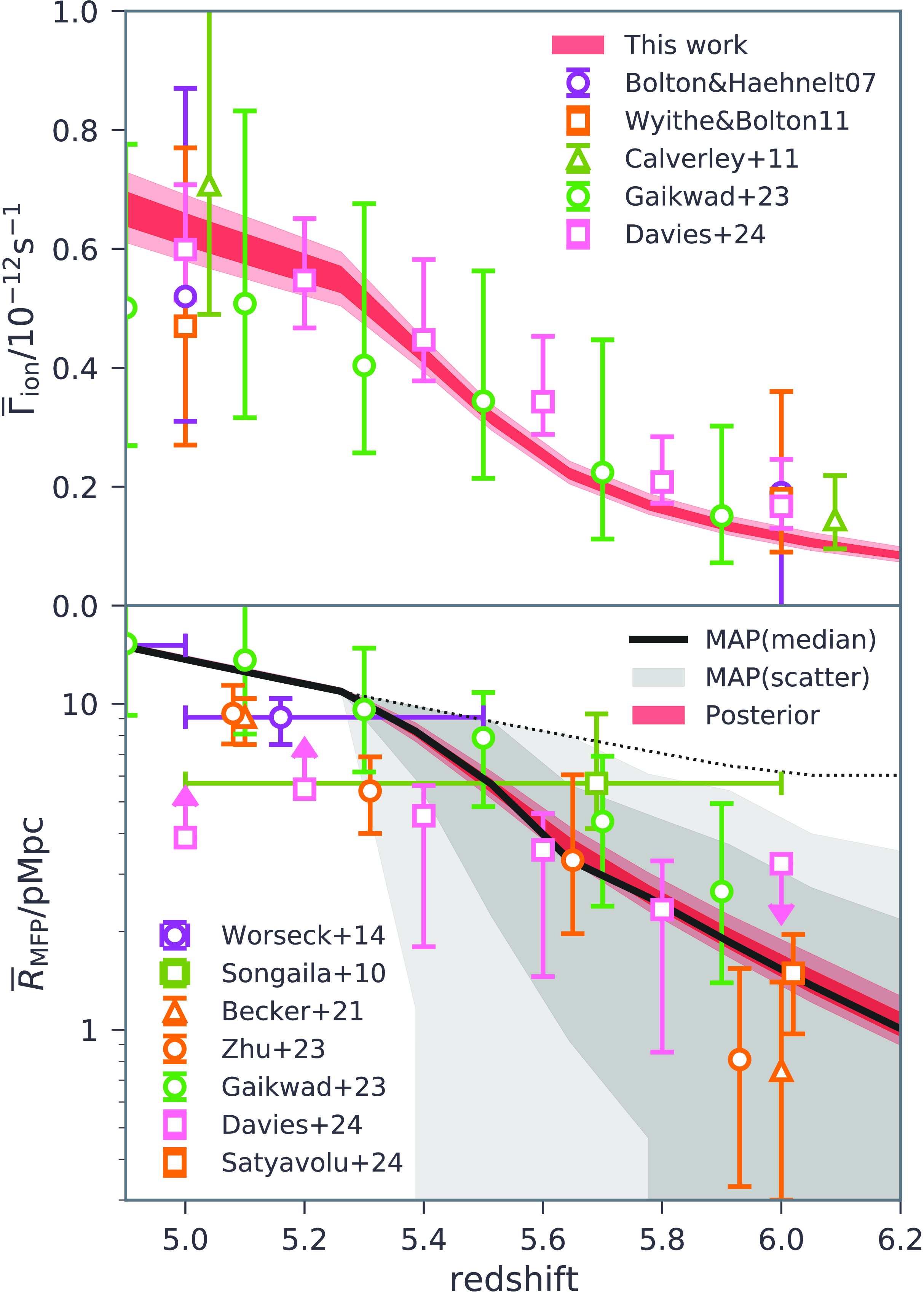
Figure 5. The posterior of our fiducial model in the space of the mean photo-ionisation rate (top panel) and proper mean free path (bottom panel). As in the previous figure, the dark (light) shaded region corresponds to 68% (95%) C.I. In the lower panel, we additionally show the volume distribution of the MFPs from the MAP model (median and scatters). The dotted line indicates the assumed $R_\textrm{MFP, LLS}$
. Various previous estimates from the forests (Bolton & Haehnelt Reference Bolton and Haehnelt2007; Wyithe & Bolton Reference Wyithe and Bolton2011; Calverley et al. Reference Calverley, Becker, Haehnelt and Bolton2011; Worseck et al. Reference Worseck2014; Songaila & Cowie Reference Songaila and Cowie2010; Becker et al. Reference Becker, D’Aloisio, Christenson, Zhu, Worseck and Bolton2021; Gaikwad et al. Reference Gaikwad2023; Zhu et al. Reference Zhu2023; Davies et al. Reference Davies2024; Satyavolu et al. Reference Satyavolu, Kulkarni, Keating and Haehnelt2024) are also shown with their 68% error bars. Our results are in general agreement with these independent estimates, despite not having used them in the inference.
$R_\textrm{MFP, LLS}$
. Various previous estimates from the forests (Bolton & Haehnelt Reference Bolton and Haehnelt2007; Wyithe & Bolton Reference Wyithe and Bolton2011; Calverley et al. Reference Calverley, Becker, Haehnelt and Bolton2011; Worseck et al. Reference Worseck2014; Songaila & Cowie Reference Songaila and Cowie2010; Becker et al. Reference Becker, D’Aloisio, Christenson, Zhu, Worseck and Bolton2021; Gaikwad et al. Reference Gaikwad2023; Zhu et al. Reference Zhu2023; Davies et al. Reference Davies2024; Satyavolu et al. Reference Satyavolu, Kulkarni, Keating and Haehnelt2024) are also shown with their 68% error bars. Our results are in general agreement with these independent estimates, despite not having used them in the inference.
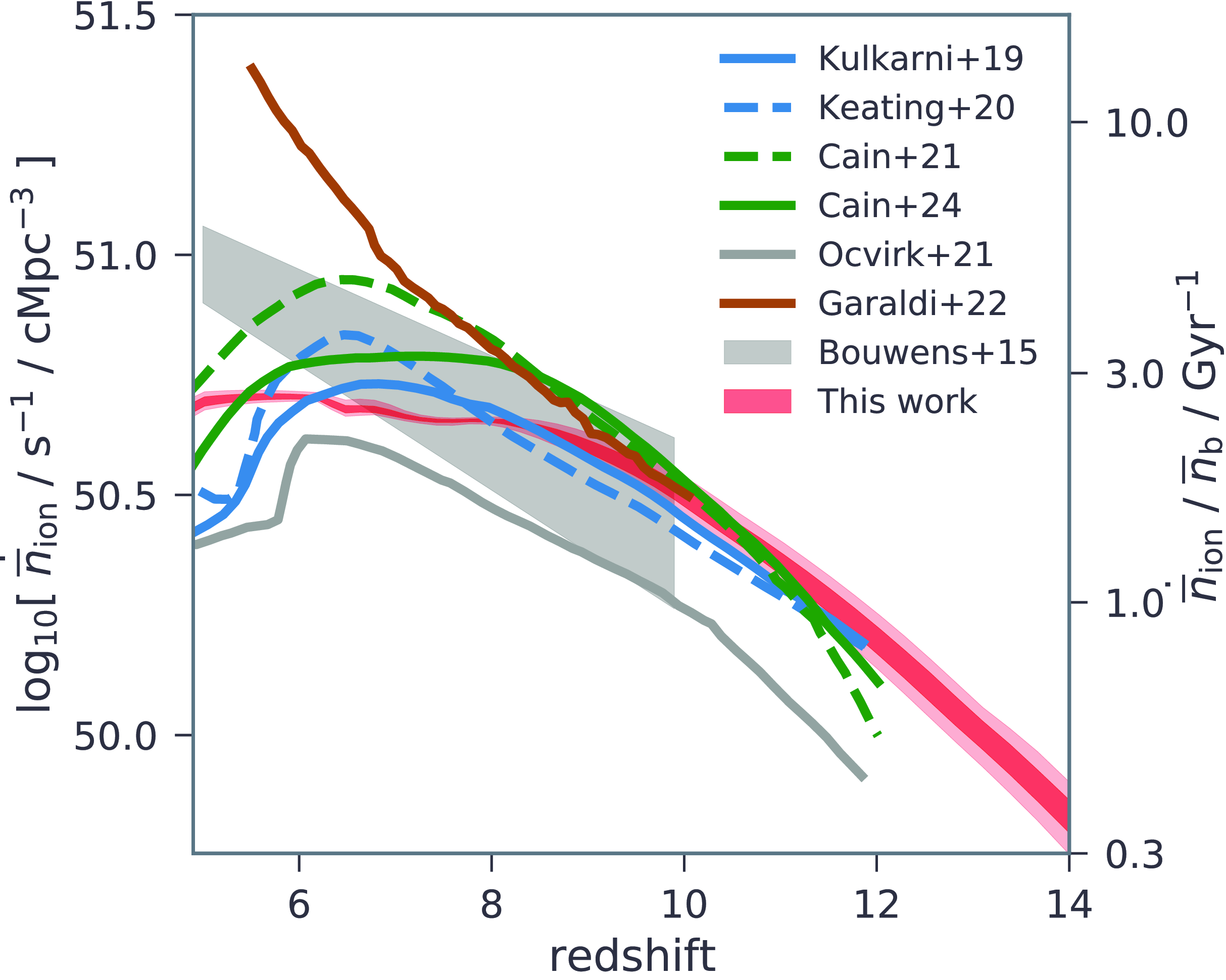
Figure 6. The inferred UV ionising emissivity, $\dot{\overline{n}}_\textrm{ion}$
. On the left axis we denote the number of ionizing photons per time per comoving volume, while on the right axis we show the number of ionizing photons per time per baryon. As in the previous figure, the dark (light) shaded red region corresponds to 68% (95%) C.I. For comparison, we include other estimates from: (i) simulations tuned to match the forest opacity distributions (Kulkarni et al. Reference Kulkarni, Keating, Haehnelt, Bosman, Puchwein, Chardin and Aubert2019; Keating et al. Reference Keating, Weinberger, Kulkarni, Haehnelt, Chardin and Aubert2020; Cain et al. Reference Cain, D’Aloisio, Gangolli and Becker2021); (ii) coupled hydrodynamic and radiative-transfer simulations (Garaldi et al. Reference Garaldi, Kannan, Smith, Springel, Pakmor, Vogelsberger and Hernquist2022; Ocvirk et al. Reference Ocvirk, Lewis, Gillet, Chardin, Aubert, Deparis and Thélie2021); and (iii) a simple empirical relation based on assuming a constant escape fraction and SFRD extrapolated down to a fixed limiting magnitude of
$\dot{\overline{n}}_\textrm{ion}$
. On the left axis we denote the number of ionizing photons per time per comoving volume, while on the right axis we show the number of ionizing photons per time per baryon. As in the previous figure, the dark (light) shaded red region corresponds to 68% (95%) C.I. For comparison, we include other estimates from: (i) simulations tuned to match the forest opacity distributions (Kulkarni et al. Reference Kulkarni, Keating, Haehnelt, Bosman, Puchwein, Chardin and Aubert2019; Keating et al. Reference Keating, Weinberger, Kulkarni, Haehnelt, Chardin and Aubert2020; Cain et al. Reference Cain, D’Aloisio, Gangolli and Becker2021); (ii) coupled hydrodynamic and radiative-transfer simulations (Garaldi et al. Reference Garaldi, Kannan, Smith, Springel, Pakmor, Vogelsberger and Hernquist2022; Ocvirk et al. Reference Ocvirk, Lewis, Gillet, Chardin, Aubert, Deparis and Thélie2021); and (iii) a simple empirical relation based on assuming a constant escape fraction and SFRD extrapolated down to a fixed limiting magnitude of $M_\textrm{UV}=-13$
(Bouwens et al. Reference Bouwens, Illingworth, Oesch, Caruana, Holwerda, Smit and Wilkins2015a).
$M_\textrm{UV}=-13$
(Bouwens et al. Reference Bouwens, Illingworth, Oesch, Caruana, Holwerda, Smit and Wilkins2015a).
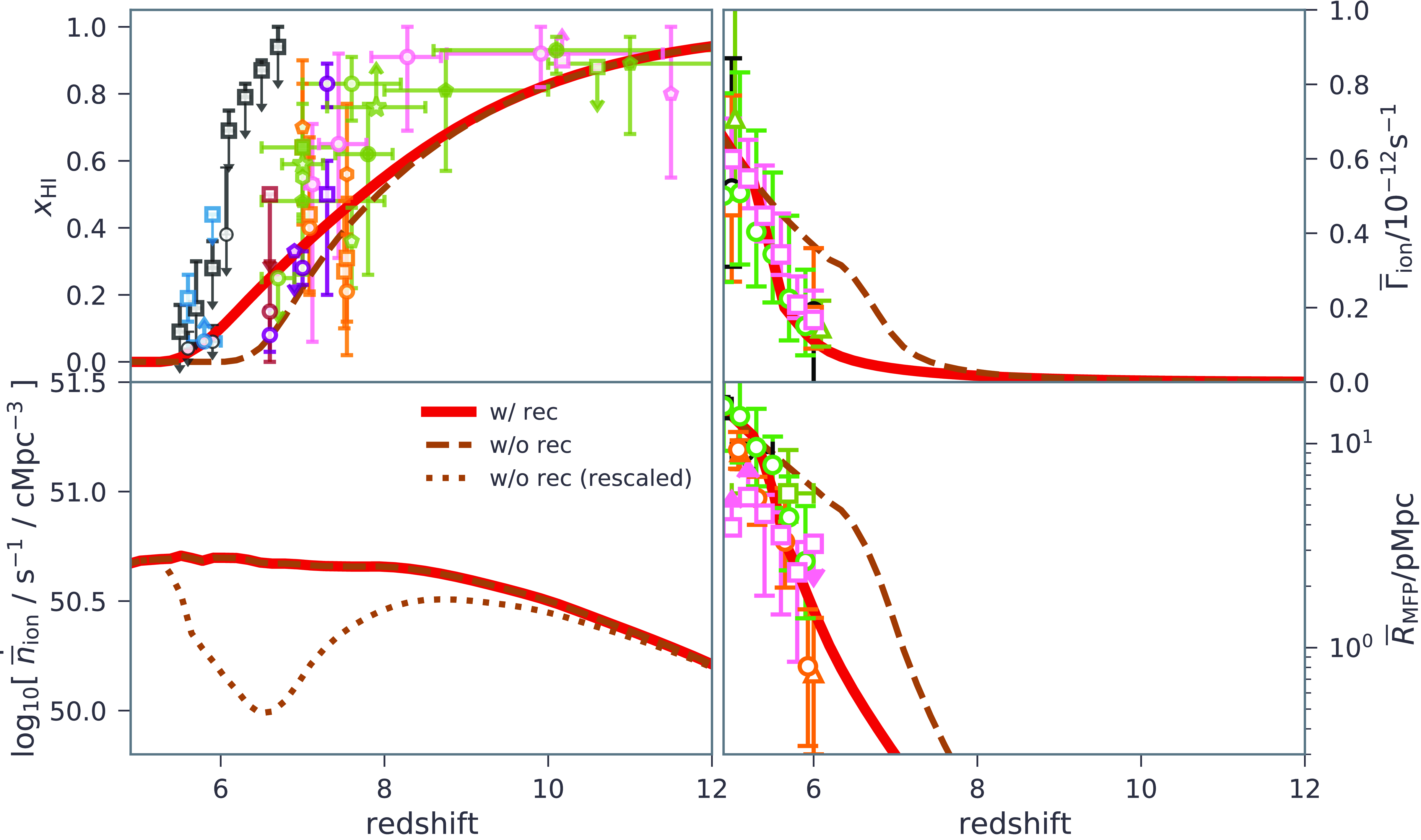
Figure 7. Comparison of the MAP model with and without recombinations. Clockwise from the upper left panel, we show the mean EoR history, photoionisation rate, proper MFP and ionizing emissivity. In the bottom left panel we also show the emissivity rescaled by the ratio of $\overline{\Gamma}_\textrm{ion}$
from w/ rec to that from w/o rec, roughly mimicking what would be required for the emissivity to compensate for the missing recombinations.
$\overline{\Gamma}_\textrm{ion}$
from w/ rec to that from w/o rec, roughly mimicking what would be required for the emissivity to compensate for the missing recombinations.
In the figure we also show several independent estimates from the literature. These come from: (i) adjusting simulated Ly $\alpha$
optical depths to match the observed flux evolution (e.g., Bolton & Haehnelt Reference Bolton and Haehnelt2007; (ii) estimating the column-density evolution of HI absorbers (Songaila & Cowie Reference Songaila and Cowie2010); (iii) modelling the size evolution of quasar near zones (Wyithe & Bolton Reference Wyithe and Bolton2011); (iv) modelling flux profiles around near zones (Calverley et al. Reference Calverley, Becker, Haehnelt and Bolton2011; Worseck et al. Reference Worseck2014; Becker et al. Reference Becker, D’Aloisio, Christenson, Zhu, Worseck and Bolton2021; Zhu et al. Reference Zhu2023; Satyavolu et al. Reference Satyavolu, Kulkarni, Keating and Haehnelt2024); and (v) co-varying the MFP and UVB to match forest fluctuations independently at each redshift (Davies et al. Reference Davies2024; Gaikwad et al. Reference Gaikwad2023). Our results are generally in good agreement with these independent estimates, despite the fact that we do not use them in our analysis. Our recovered MFP at
$\alpha$
optical depths to match the observed flux evolution (e.g., Bolton & Haehnelt Reference Bolton and Haehnelt2007; (ii) estimating the column-density evolution of HI absorbers (Songaila & Cowie Reference Songaila and Cowie2010); (iii) modelling the size evolution of quasar near zones (Wyithe & Bolton Reference Wyithe and Bolton2011); (iv) modelling flux profiles around near zones (Calverley et al. Reference Calverley, Becker, Haehnelt and Bolton2011; Worseck et al. Reference Worseck2014; Becker et al. Reference Becker, D’Aloisio, Christenson, Zhu, Worseck and Bolton2021; Zhu et al. Reference Zhu2023; Satyavolu et al. Reference Satyavolu, Kulkarni, Keating and Haehnelt2024); and (v) co-varying the MFP and UVB to match forest fluctuations independently at each redshift (Davies et al. Reference Davies2024; Gaikwad et al. Reference Gaikwad2023). Our results are generally in good agreement with these independent estimates, despite the fact that we do not use them in our analysis. Our recovered MFP at $z\sim6$
is on the upper end of the 68% error bars from Becker et al. (Reference Becker, D’Aloisio, Christenson, Zhu, Worseck and Bolton2021), Zhu et al. (Reference Zhu2023) This mild tension could point to additional systematics in these observational interpretations (see more in Satyavolu et al. Reference Satyavolu, Kulkarni, Keating and Haehnelt2024) and/or missing physics in our models, such as gas relaxation (e.g., Park et al. Reference Park and Shapiro2016; D’Aloisio 2020) or the inhomogeneous post I-front temperature (e.g., D’Aloisio et al. Reference D’Aloisio, McQuinn, Maupin, Davies, Trac, Fuller and Upton Sanderbeck2019; Davies et al. Reference Davies, Mutch, Qin, Mesinger, Poole and Wyithe2019). We plan on investigating these effects in future work.
$z\sim6$
is on the upper end of the 68% error bars from Becker et al. (Reference Becker, D’Aloisio, Christenson, Zhu, Worseck and Bolton2021), Zhu et al. (Reference Zhu2023) This mild tension could point to additional systematics in these observational interpretations (see more in Satyavolu et al. Reference Satyavolu, Kulkarni, Keating and Haehnelt2024) and/or missing physics in our models, such as gas relaxation (e.g., Park et al. Reference Park and Shapiro2016; D’Aloisio 2020) or the inhomogeneous post I-front temperature (e.g., D’Aloisio et al. Reference D’Aloisio, McQuinn, Maupin, Davies, Trac, Fuller and Upton Sanderbeck2019; Davies et al. Reference Davies, Mutch, Qin, Mesinger, Poole and Wyithe2019). We plan on investigating these effects in future work.
In the bottom panel of Fig. 5, we additionally present the volume distribution of the MFPs derived from our MAP model. The black curve represents the median while the grey shaded regions indicate 68% and 95% of the volume distribution. We see that 68% of the volume has an MFP determined by $R_\textrm{MFP, EoR}$
at
$R_\textrm{MFP, EoR}$
at $z\sim5.5$
, even though reionisation completes at
$z\sim5.5$
, even though reionisation completes at $z=5.44$
. This finding underscores that the assumed functional form of
$z=5.44$
. This finding underscores that the assumed functional form of $R_\textrm{MFP, LLS}$
likely has a minor impact on the MFP at these EoR redshifts. Nevertheless in future work we will additionally sample the uncertainties in the mean and scatter of
$R_\textrm{MFP, LLS}$
likely has a minor impact on the MFP at these EoR redshifts. Nevertheless in future work we will additionally sample the uncertainties in the mean and scatter of $R_\textrm{MFP, LLS}$
.
$R_\textrm{MFP, LLS}$
.
4.4 UV ionising emissivity
In Fig. 6, we present the inferred ionising emissivity evolution, $\dot{\overline{n}}_\textrm{ion}(z)$
(c.f. equation 3). Unlike many previous studies (e.g., Kulkarni et al. Reference Kulkarni, Keating, Haehnelt, Bosman, Puchwein, Chardin and Aubert2019; Keating et al. Reference Keating, Weinberger, Kulkarni, Haehnelt, Chardin and Aubert2020; Cain et al. Reference Cain, D’Aloisio, Gangolli and Becker2021), we reproduce the Ly
$\dot{\overline{n}}_\textrm{ion}(z)$
(c.f. equation 3). Unlike many previous studies (e.g., Kulkarni et al. Reference Kulkarni, Keating, Haehnelt, Bosman, Puchwein, Chardin and Aubert2019; Keating et al. Reference Keating, Weinberger, Kulkarni, Haehnelt, Chardin and Aubert2020; Cain et al. Reference Cain, D’Aloisio, Gangolli and Becker2021), we reproduce the Ly $\alpha$
opacity distribution without requiring a sharp drop in the emissivity at
$\alpha$
opacity distribution without requiring a sharp drop in the emissivity at $z\lesssim7$
. Such a rapid drop in the emissivity would be difficult to reconcile with the more gradual evolution implied by observations of galaxy UV LFs (e.g., Bouwens et al. Reference Bouwens, Illingworth, Oesch, Caruana, Holwerda, Smit and Wilkins2015a), as it requires either fast evolving feedback in faint galaxies (e.g., Ocvirk et al. Reference Ocvirk, Lewis, Gillet, Chardin, Aubert, Deparis and Thélie2021; though see e.g., Sobacchi & Mesinger Reference Sobacchi and Mesinger2014; Katz et al. Reference Katz2020) or in their ionising escape fractions. Even under both such putative scenarios, it is difficult to physically justify cosmological evolution that is more rapid than characteristic time-scales during this epoch which are generally
$z\lesssim7$
. Such a rapid drop in the emissivity would be difficult to reconcile with the more gradual evolution implied by observations of galaxy UV LFs (e.g., Bouwens et al. Reference Bouwens, Illingworth, Oesch, Caruana, Holwerda, Smit and Wilkins2015a), as it requires either fast evolving feedback in faint galaxies (e.g., Ocvirk et al. Reference Ocvirk, Lewis, Gillet, Chardin, Aubert, Deparis and Thélie2021; though see e.g., Sobacchi & Mesinger Reference Sobacchi and Mesinger2014; Katz et al. Reference Katz2020) or in their ionising escape fractions. Even under both such putative scenarios, it is difficult to physically justify cosmological evolution that is more rapid than characteristic time-scales during this epoch which are generally $\gtrsim$
200 Myrs (e.g., the duration of the EoR, halo dynamical and/or sound crossing times; c.f. Sobacchi & Mesinger Reference Sobacchi and Mesinger2013). As discussed in Section 4.2, one possible explanation is that simulating the end stages of the EoR requires very large-scale and very high-resolution hydrodynamic simulations to track the rapid evolution of self-shielding in the IGM and the strong spatial correlation between ionizing sinks and sources. Our calibrated sub-grid approach could allow us to capture the relevant recombination physics without requiring very high resolution (Sobacchi & Mesinger Reference Sobacchi and Mesinger2014).
$\gtrsim$
200 Myrs (e.g., the duration of the EoR, halo dynamical and/or sound crossing times; c.f. Sobacchi & Mesinger Reference Sobacchi and Mesinger2013). As discussed in Section 4.2, one possible explanation is that simulating the end stages of the EoR requires very large-scale and very high-resolution hydrodynamic simulations to track the rapid evolution of self-shielding in the IGM and the strong spatial correlation between ionizing sinks and sources. Our calibrated sub-grid approach could allow us to capture the relevant recombination physics without requiring very high resolution (Sobacchi & Mesinger Reference Sobacchi and Mesinger2014).
To better quantify this claim, we rerun the MAP model, turning off inhomogeneous recombinations. Fig. 7 shows the predicted mean EoR history, photoionisation rate, MFP and ionizing emissivity. In the absence of sub-grid recombinations, the end of reionisation progresses significantly more rapidly, leading to a correspondingly sharp rise in both the MFP and photo-ionisation rate (see also Sobacchi & Mesinger Reference Sobacchi and Mesinger2014). Since our models fix the post-reionisation MFP to $R_\textrm{MFP, LLS}$
, these quantities eventually asymptote to the same values as in the fiducial run. In the emissivity sub-panel, we also adjust the emissivity by rescaling it with the ratio of
$R_\textrm{MFP, LLS}$
, these quantities eventually asymptote to the same values as in the fiducial run. In the emissivity sub-panel, we also adjust the emissivity by rescaling it with the ratio of $\overline{\Gamma}_\textrm{ion}$
from w/ rec to that from w/o rec. We see that by matching the UVB (which roughly corresponds to what forest observations would require for the w/o rec case), the emissivity would need to decrease rapidly during the second half of the EoR, countering the premature rise in the MFP caused by the lack of recombinations. This lends further credibility to our claim that unresolved, inhomogeneous recombinations are responsible (at least in part) for the rapid drop in the emissivity required by some large-scale hydro simulations in order to match the forest data.
$\overline{\Gamma}_\textrm{ion}$
from w/ rec to that from w/o rec. We see that by matching the UVB (which roughly corresponds to what forest observations would require for the w/o rec case), the emissivity would need to decrease rapidly during the second half of the EoR, countering the premature rise in the MFP caused by the lack of recombinations. This lends further credibility to our claim that unresolved, inhomogeneous recombinations are responsible (at least in part) for the rapid drop in the emissivity required by some large-scale hydro simulations in order to match the forest data.
We note from Fig. 6 that our inferred emissivity is consistent with simple estimates assuming a constant escape fraction and integrating the observed UV LFs down to $M_\textrm{UV} = -13$
. This is somewhat coincidental, since in our fiducial model more than half of the ionizing photons are provided by galaxies fainter than
$M_\textrm{UV} = -13$
. This is somewhat coincidental, since in our fiducial model more than half of the ionizing photons are provided by galaxies fainter than $M_\textrm{UV} \gt -13$
due to a strong
$M_\textrm{UV} \gt -13$
due to a strong $M_\textrm{UV}$
-dependence of the ionizing escape fraction (see later Fig. 10). As discussed further in Section 5, the forest data combined with UV LFs strongly constrain the redshift evolution of the EoR and the ionizing emissivity. However, determining which galaxies produce the ionizing photons responsible is more model dependent.
$M_\textrm{UV}$
-dependence of the ionizing escape fraction (see later Fig. 10). As discussed further in Section 5, the forest data combined with UV LFs strongly constrain the redshift evolution of the EoR and the ionizing emissivity. However, determining which galaxies produce the ionizing photons responsible is more model dependent.
4.5 Effective clumping factor in HII regions
Modelling the complex interplay between ionizing sinks and sources during the EoR is best achieved with large-scale numerical simulations. However, simple analytic estimates of the EoR history can be very convenient and help build physical intuition. A common choice is the following (e.g., Bouwens et al. Reference Bouwens, Illingworth, Oesch, Caruana, Holwerda, Smit and Wilkins2015a):
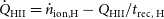 \begin{equation} \dot{Q}_\textrm{HII} = \dot{n}_\textrm{ion,H} - Q_\textrm{HII} / t_\textrm{rec, H}\end{equation}
where
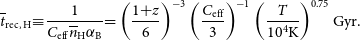 \begin{equation} \overline{t}_\textrm{rec, H} {\equiv} \frac{1}{C_\textrm{eff} \overline{n}_\textrm{H}\alpha_\textrm{B}} {=} \left(\frac{1{+}z}{6}\right)^{-3}\left(\frac{C_\textrm{eff}}{3}\right)^{-1}\left(\frac{T}{10^4\textrm{K}}\right)^{0.75}\textrm{Gyr} .\end{equation}
Here, $Q_\textrm{HII} {\sim} 1-\overline{x}_\textrm{HI}$
and
$Q_\textrm{HII} {\sim} 1-\overline{x}_\textrm{HI}$
and $\dot{Q}_\textrm{HII}$
are the volume filling factors of HII regions and its growth rate while
$\dot{Q}_\textrm{HII}$
are the volume filling factors of HII regions and its growth rate while $t_\textrm{rec, H}$
is a characteristic recombination time-scale parameterised by an ‘effective’ clumping factor,
$t_\textrm{rec, H}$
is a characteristic recombination time-scale parameterised by an ‘effective’ clumping factor, $C_\textrm{eff}$
. The first term on the right-hand side of equation (11) is the ionizing emissivity per hydrogen atom while the second term approximates the global recombination rate per hydrogen atom. This equation is especially useful in high-redshift galaxy studies, as it allows us to connect the ionizing emissivity from galaxies to the EoR history simply by assuming some value of
$C_\textrm{eff}$
. The first term on the right-hand side of equation (11) is the ionizing emissivity per hydrogen atom while the second term approximates the global recombination rate per hydrogen atom. This equation is especially useful in high-redshift galaxy studies, as it allows us to connect the ionizing emissivity from galaxies to the EoR history simply by assuming some value of $C_\textrm{eff}$
to capture the impact of recombinations. Common choices for
$C_\textrm{eff}$
to capture the impact of recombinations. Common choices for $C_\textrm{eff}$
range from
$C_\textrm{eff}$
range from $\sim$
1–10 (e.g., Bouwens et al. Reference Bouwens, Illingworth, Oesch, Caruana, Holwerda, Smit and Wilkins2015a; Mason et al. Reference Mason, Treu, Dijkstra, Mesinger, Trenti, Pentericci, de Barros and Vanzella2018; Davies et al. Reference Davies, Mutch, Qin, Mesinger, Poole and Wyithe2019; Bruton et al. Reference Bruton, Lin, Scarlata and Hayes2023).
$\sim$
1–10 (e.g., Bouwens et al. Reference Bouwens, Illingworth, Oesch, Caruana, Holwerda, Smit and Wilkins2015a; Mason et al. Reference Mason, Treu, Dijkstra, Mesinger, Trenti, Pentericci, de Barros and Vanzella2018; Davies et al. Reference Davies, Mutch, Qin, Mesinger, Poole and Wyithe2019; Bruton et al. Reference Bruton, Lin, Scarlata and Hayes2023).
One can compute the recombination rate in a given patch of the IGM by defining $C_\textrm{eff} = \langle n_\textrm{HII}^2 \rangle / \langle n_\textrm{HII} \rangle^2$
, where the averaging is performed over the ionised hydrogen (accounting for self-shielding and using local values of temperature and ionisation rates; e.g. Finlator et al. Reference Finlator, Peng Oh, Özel and Davé2012) with
$C_\textrm{eff} = \langle n_\textrm{HII}^2 \rangle / \langle n_\textrm{HII} \rangle^2$
, where the averaging is performed over the ionised hydrogen (accounting for self-shielding and using local values of temperature and ionisation rates; e.g. Finlator et al. Reference Finlator, Peng Oh, Özel and Davé2012) with $n_\textrm{HII}$
being the local HII density. However, when estimating the global recombination rate to be used in equation (11) there is not an obvious way of defining
$n_\textrm{HII}$
being the local HII density. However, when estimating the global recombination rate to be used in equation (11) there is not an obvious way of defining $C_\textrm{eff}$
in terms of other global IGM quantities. In particular, ionizing sources and sinks are strongly correlated on large scales. Recombinations preferentially occur in regions proximate to galaxies that were the first to reionise, which have biased, time-evolving, and spatially fluctuating properties.
$C_\textrm{eff}$
in terms of other global IGM quantities. In particular, ionizing sources and sinks are strongly correlated on large scales. Recombinations preferentially occur in regions proximate to galaxies that were the first to reionise, which have biased, time-evolving, and spatially fluctuating properties.
Here, we investigate what choice of $C_\textrm{eff}$
can give the same EoR history as the MAP parameter set in our fiducial model. Specifically, we assume the EoR history and emissivity of our MAP model (c.f. Figs. 4 and 6), and solve for
$C_\textrm{eff}$
can give the same EoR history as the MAP parameter set in our fiducial model. Specifically, we assume the EoR history and emissivity of our MAP model (c.f. Figs. 4 and 6), and solve for $C_\textrm{eff}(z)$
using equation (11). The resulting effective clumping factor is plotted as a red curve in the bottom panel of Fig. 8. We see
$C_\textrm{eff}(z)$
using equation (11). The resulting effective clumping factor is plotted as a red curve in the bottom panel of Fig. 8. We see $C_\textrm{eff}$
starts around unityFootnote
j
and then rises rapidly towards the late stages of reionisation when ionisation fronts penetrate deeper into overdensities (e.g., Furlanetto, Oh, & Briggs Reference Furlanetto, Oh and Briggs2006; Finlator et al. Reference Finlator, Peng Oh, Özel and Davé2012; Sobacchi & Mesinger Reference Sobacchi and Mesinger2014; Cain et al. Reference Cain, D’Aloisio, Lopez, Gangolli and Roth2024; Davies, Bosman, & Furlanetto Reference Davies, Bosman and Furlanetto2024).
$C_\textrm{eff}$
starts around unityFootnote
j
and then rises rapidly towards the late stages of reionisation when ionisation fronts penetrate deeper into overdensities (e.g., Furlanetto, Oh, & Briggs Reference Furlanetto, Oh and Briggs2006; Finlator et al. Reference Finlator, Peng Oh, Özel and Davé2012; Sobacchi & Mesinger Reference Sobacchi and Mesinger2014; Cain et al. Reference Cain, D’Aloisio, Lopez, Gangolli and Roth2024; Davies, Bosman, & Furlanetto Reference Davies, Bosman and Furlanetto2024).
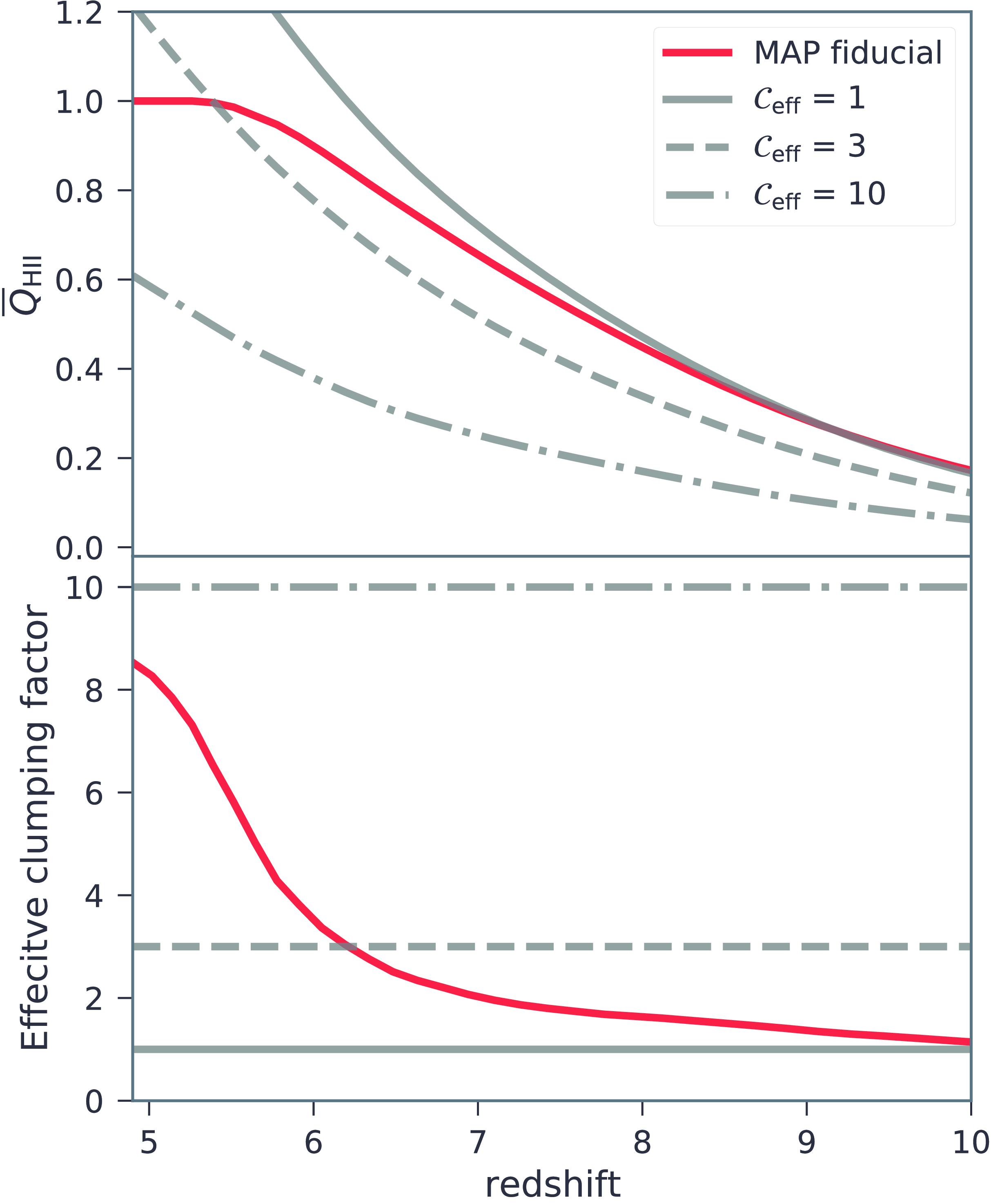
Figure 8.
Top panel: Evolution of the HII filling factor from the MAP model (red curve), together with analytic estimates using equation (11) assuming the same mean ionizing emissivity as the MAP but taking a constant ‘clumping factor’. Curves corresponding to $C_\textrm{eff}$
=1, 3, 10 are shown in grey. Bottom panel: the effective clumping factor obtained by solving equation (11) for
$C_\textrm{eff}$
=1, 3, 10 are shown in grey. Bottom panel: the effective clumping factor obtained by solving equation (11) for $C_\textrm{eff}(z)$
when assuming the EoR history and emissivity from the MAP model.
$C_\textrm{eff}(z)$
when assuming the EoR history and emissivity from the MAP model.
Fundamentally, $C_\textrm{eff}$
cannot be a constant during the EoR. We illustrate EoR histories resulting from common assumptions of a constant
$C_\textrm{eff}$
cannot be a constant during the EoR. We illustrate EoR histories resulting from common assumptions of a constant $C_\textrm{eff}$
= 1, 3, 10 in the top panel of Fig. 8. All curves assume the same emissivity as the MAP. However, no constant choice of
$C_\textrm{eff}$
= 1, 3, 10 in the top panel of Fig. 8. All curves assume the same emissivity as the MAP. However, no constant choice of $C_\textrm{eff}$
can reproduce the EoR history of the MAP (red curve).
$C_\textrm{eff}$
can reproduce the EoR history of the MAP (red curve).
We offer a fit for $C_\textrm{eff}(z)$
using a rational function (equation 10) with coefficients
$C_\textrm{eff}(z)$
using a rational function (equation 10) with coefficients $\{m_0,m_1,m_2,m_3,n_0,n_1,n_2,n_3\}$
= {238.9, −94.35, 11.76, −0.404, 22.6, −3.97, −0.877, 0.1636}. This can be used in analytic models to approximate the EoR history resulting from a given emissivity. In future work we will quantify how sensitive this effective clumping factor is to different reionisation or emissivity models.
$\{m_0,m_1,m_2,m_3,n_0,n_1,n_2,n_3\}$
= {238.9, −94.35, 11.76, −0.404, 22.6, −3.97, −0.877, 0.1636}. This can be used in analytic models to approximate the EoR history resulting from a given emissivity. In future work we will quantify how sensitive this effective clumping factor is to different reionisation or emissivity models.
4.6 Galaxy UV LFs and scaling relations
In Fig. 9 we show the inferred UV LFs for our fiducial model. As in Fig. 4, the blue shaded regions correspond to our posterior without including forest data (i.e. only including UV LF data and $\tau_e$
), while the red regions additionally include the
$\tau_e$
), while the red regions additionally include the $\tau_\textrm{eff}$
distributions from XQR-30+. In the figure we also show observational estimates from both Hubble and JWST, with blue points highlighting those Hubble datasets that are used in the likelihood (see Section 3.5). The MAP model and [16, 84]th percentiles are also listed in Table A2.
$\tau_\textrm{eff}$
distributions from XQR-30+. In the figure we also show observational estimates from both Hubble and JWST, with blue points highlighting those Hubble datasets that are used in the likelihood (see Section 3.5). The MAP model and [16, 84]th percentiles are also listed in Table A2.

Figure 9. The inferred galaxy UV luminosity function. As in the previous figure, the dark (light) shaded region corresponds to 68% (95%) C.I. Observed luminosity functions are grouped into pre-JWST (light grey; Bouwens et al. Reference Bouwens2016, Reference Bouwens2015b; Finkelstein et al. Reference Finkelstein2015; Oesch et al. Reference Oesch2016, Reference Oesch, Bouwens, Illingworth, Labbé and Stefanon2018; Reference Livermore, Finkelstein and LotzLivermore, Finkelstein, & Lotz 2023; Atek et al. Reference Atek, Richard, Kneib and Schaerer2018; Ishigaki et al. Reference Ishigaki, Kawamata, Ouchi, Oguri, Shimasaku and Ono2018; Bhatawdekar et al. Reference Bhatawdekar, Conselice, Margalef-Bentabol and Duncan2019; Bouwens et al. Reference Bouwens2016; Kauttmann et al. 2022; Leethochawalit et al. Reference Leethochawalit, Roberts-Borsani, Morishita, Trenti and Treu2023) with those used in the likelihood (see Section 3.5) highlighted in dark blue, and results using recent JWST observations (dark grey; Donnan et al. Reference Donnan2023; Finkelstein et al. Reference Finkelstein2022; Harikane et al. Reference Harikane2023; Naidu et al. Reference Naidu2022; Pérez-González et al. Reference Pérez-González2023; Willott et al. Reference Willott2024).
From the figure we see that the Hubble estimates we use in the likelihood already constrain the inferred UV LFs at magnitudes brighter than −17, where we have observational estimates. Overall, the predictions also remain consistent with recent JWST measurements (e.g., Donnan et al. Reference Donnan2023; Harikane et al. Reference Harikane2023; Willott et al. Reference Willott2024), though observations at $10 \lt z\lesssim13$
appear slightly higher. At
$10 \lt z\lesssim13$
appear slightly higher. At $z\sim16$
, however, UV variability (Shen et al. Reference Shen, Vogelsberger, Boylan-Kolchin, Tacchella and Kannan2023; Nikolić et al. 2024) sourced by enhanced star formation (e.g., Qin, Balu, &Wyithe Reference Qin, Balu and Wyithe2023;Wang et al. Reference Wang, Lei, Yuan and Fan2023; Chakraborty & Choudhury Reference Chakraborty and Choudhury2024) or differences in stellar populations (e.g., Ventura et al. Reference Ventura, Qin, Balu and Wyithe2024; Yung et al. Reference Yung, Somerville, Finkelstein, Wilkins and Gardner2024) may be indeed necessary to explain the observed trends. This offset suggests that a redshift evolution in
$z\sim16$
, however, UV variability (Shen et al. Reference Shen, Vogelsberger, Boylan-Kolchin, Tacchella and Kannan2023; Nikolić et al. 2024) sourced by enhanced star formation (e.g., Qin, Balu, &Wyithe Reference Qin, Balu and Wyithe2023;Wang et al. Reference Wang, Lei, Yuan and Fan2023; Chakraborty & Choudhury Reference Chakraborty and Choudhury2024) or differences in stellar populations (e.g., Ventura et al. Reference Ventura, Qin, Balu and Wyithe2024; Yung et al. Reference Yung, Somerville, Finkelstein, Wilkins and Gardner2024) may be indeed necessary to explain the observed trends. This offset suggests that a redshift evolution in $f_*$
(or
$f_*$
(or $\tau_*$
) might also be needed in our model, similar to the adjustments made for
$\tau_*$
) might also be needed in our model, similar to the adjustments made for $f_\textrm{esc}$
(see equation 2). We will explore this further as JWST data continue to mature. On the other hand, the posteriors in blue widen greatly at fainter magnitudes, since there is no observational consensus regarding a faint-end turn-over (see also Gillet, Mesinger, &Park Reference Gillet, Mesinger and Park2020 and Atek et al. Reference Atek2024). Once we include the forest data however, the posteriors shrink significantly at the faint end of the UV LF. The forest data imply significant star formation in galaxies down to the atomic cooling limit (
$f_\textrm{esc}$
(see equation 2). We will explore this further as JWST data continue to mature. On the other hand, the posteriors in blue widen greatly at fainter magnitudes, since there is no observational consensus regarding a faint-end turn-over (see also Gillet, Mesinger, &Park Reference Gillet, Mesinger and Park2020 and Atek et al. Reference Atek2024). Once we include the forest data however, the posteriors shrink significantly at the faint end of the UV LF. The forest data imply significant star formation in galaxies down to the atomic cooling limit ( $M_\textrm{UV} \sim$
−10).
$M_\textrm{UV} \sim$
−10).
Note that the Ly $\alpha$
forest is not sensitive enough to directly distinguish between different reionisation morphologies (see section 5.3 in Q21). Therefore the preference for star formation in UV faint galaxies indirectly comes from the mean EoR history shown in Fig. 4. Abundant, faint galaxies appear earlier and evolve more slowly, compared to rare, bright galaxies (e.g., Behroozi et al. Reference Behroozi, Wechsler, Hearin and Conroy2019). Therefore they more naturally drive the kind of slower reionisation histories with a ‘soft-landing’, which is preferred by the Ly
$\alpha$
forest is not sensitive enough to directly distinguish between different reionisation morphologies (see section 5.3 in Q21). Therefore the preference for star formation in UV faint galaxies indirectly comes from the mean EoR history shown in Fig. 4. Abundant, faint galaxies appear earlier and evolve more slowly, compared to rare, bright galaxies (e.g., Behroozi et al. Reference Behroozi, Wechsler, Hearin and Conroy2019). Therefore they more naturally drive the kind of slower reionisation histories with a ‘soft-landing’, which is preferred by the Ly $\alpha$
forest. Yet, given sufficient flexibility in assigning ionizing escape fractions, one could in principle force a bright-galaxy-dominated EoR to have the same history as the one shown in Fig. 4, which is driven by faint galaxies. This, in practice, is constrained by the fact that the escape fraction cannot exceed unity, and that bright galaxies reside in the exponential tail of the mass function. Thus very extreme evolutions in the ionizing escape fractions, exceeding unity, would be required for our model to have a ‘bright galaxy dominated EoR’ that is consistent with Ly
$\alpha$
forest. Yet, given sufficient flexibility in assigning ionizing escape fractions, one could in principle force a bright-galaxy-dominated EoR to have the same history as the one shown in Fig. 4, which is driven by faint galaxies. This, in practice, is constrained by the fact that the escape fraction cannot exceed unity, and that bright galaxies reside in the exponential tail of the mass function. Thus very extreme evolutions in the ionizing escape fractions, exceeding unity, would be required for our model to have a ‘bright galaxy dominated EoR’ that is consistent with Ly $\alpha$
forest data. Such models are not in our prior volume.
$\alpha$
forest data. Such models are not in our prior volume.
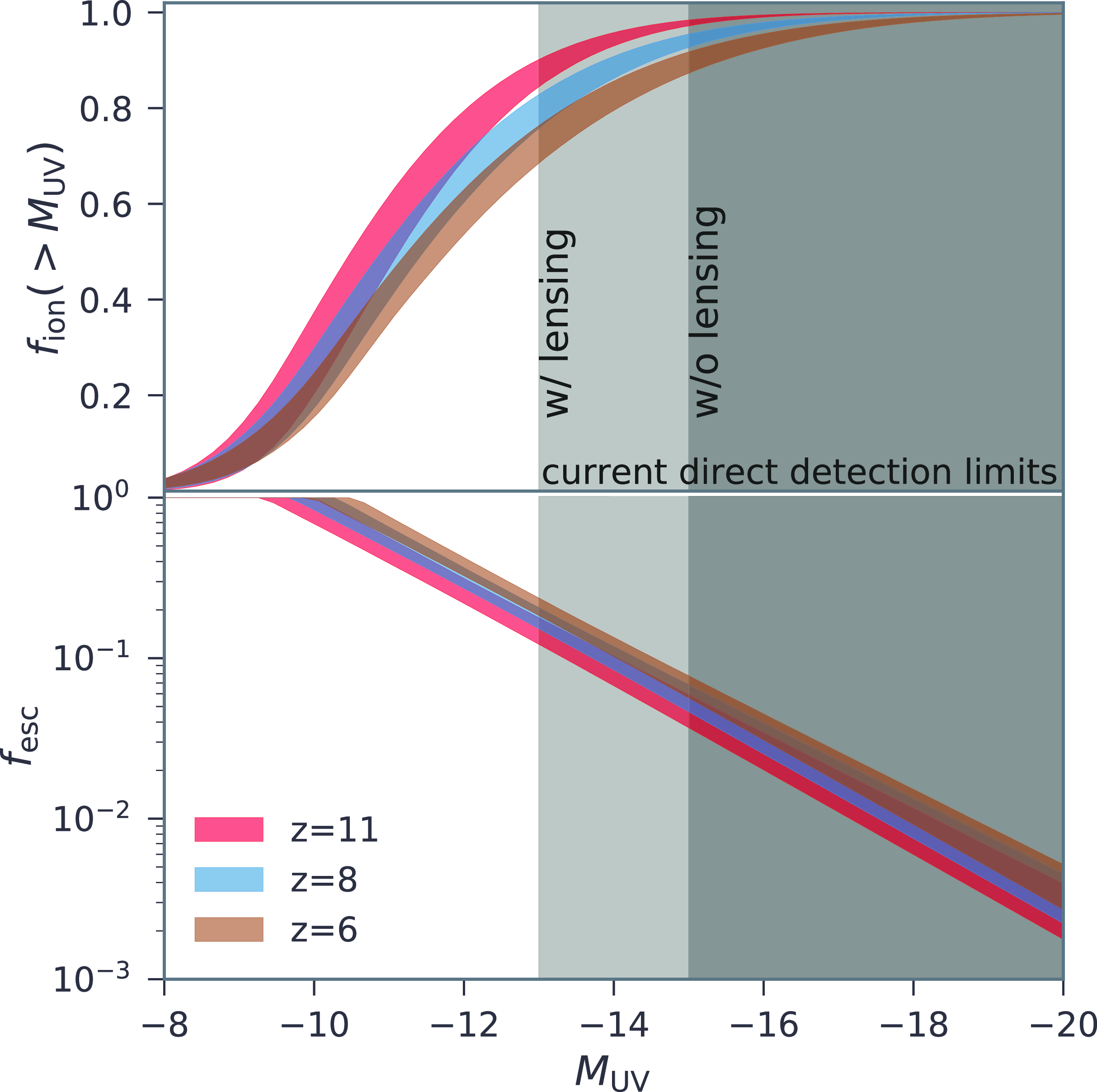
Figure 10. The inferred (68% C.I.) ionizing contribution of galaxies as a function of their UV magnitudes at $z=6$
, 8 and 11. The top panel shows the normalised cumulative number of ionizing photons while the bottom panel shows the escape fraction. Our results imply reionisation is driven by faint galaxies, far below current direct detection limits (roughly corresponding to the grey shaded region).
$z=6$
, 8 and 11. The top panel shows the normalised cumulative number of ionizing photons while the bottom panel shows the escape fraction. Our results imply reionisation is driven by faint galaxies, far below current direct detection limits (roughly corresponding to the grey shaded region).
We further quantify the contribution of faint galaxies to the EoR in Fig. 10. In the top panel we plot the CDF of the galaxies contributing to the ionizing background at $z=$
6, 8, and 11 as functions of
$z=$
6, 8, and 11 as functions of $M_\textrm{UV}$
. There is a mild evolution with redshift, but in general we find that galaxies fainter than
$M_\textrm{UV}$
. There is a mild evolution with redshift, but in general we find that galaxies fainter than $M_\textrm{UV} \gtrsim -12$
contribute more than half of the ionizing photons that have reionised the universe. Galaxies above the current direct detection limits of
$M_\textrm{UV} \gtrsim -12$
contribute more than half of the ionizing photons that have reionised the universe. Galaxies above the current direct detection limits of $M_\textrm{UV} \lesssim -15$
only contribute a few percent to the ionizing photon budget with gravitational lensing enabling the detection of even fainter sources and extending constraints on their contribution (e.g., Vanzella et al. Reference Vanzella2023, Reference Vanzella2024). This highlights the power of the IGM as a democratic probe of the emissivity of all galaxies.
$M_\textrm{UV} \lesssim -15$
only contribute a few percent to the ionizing photon budget with gravitational lensing enabling the detection of even fainter sources and extending constraints on their contribution (e.g., Vanzella et al. Reference Vanzella2023, Reference Vanzella2024). This highlights the power of the IGM as a democratic probe of the emissivity of all galaxies.
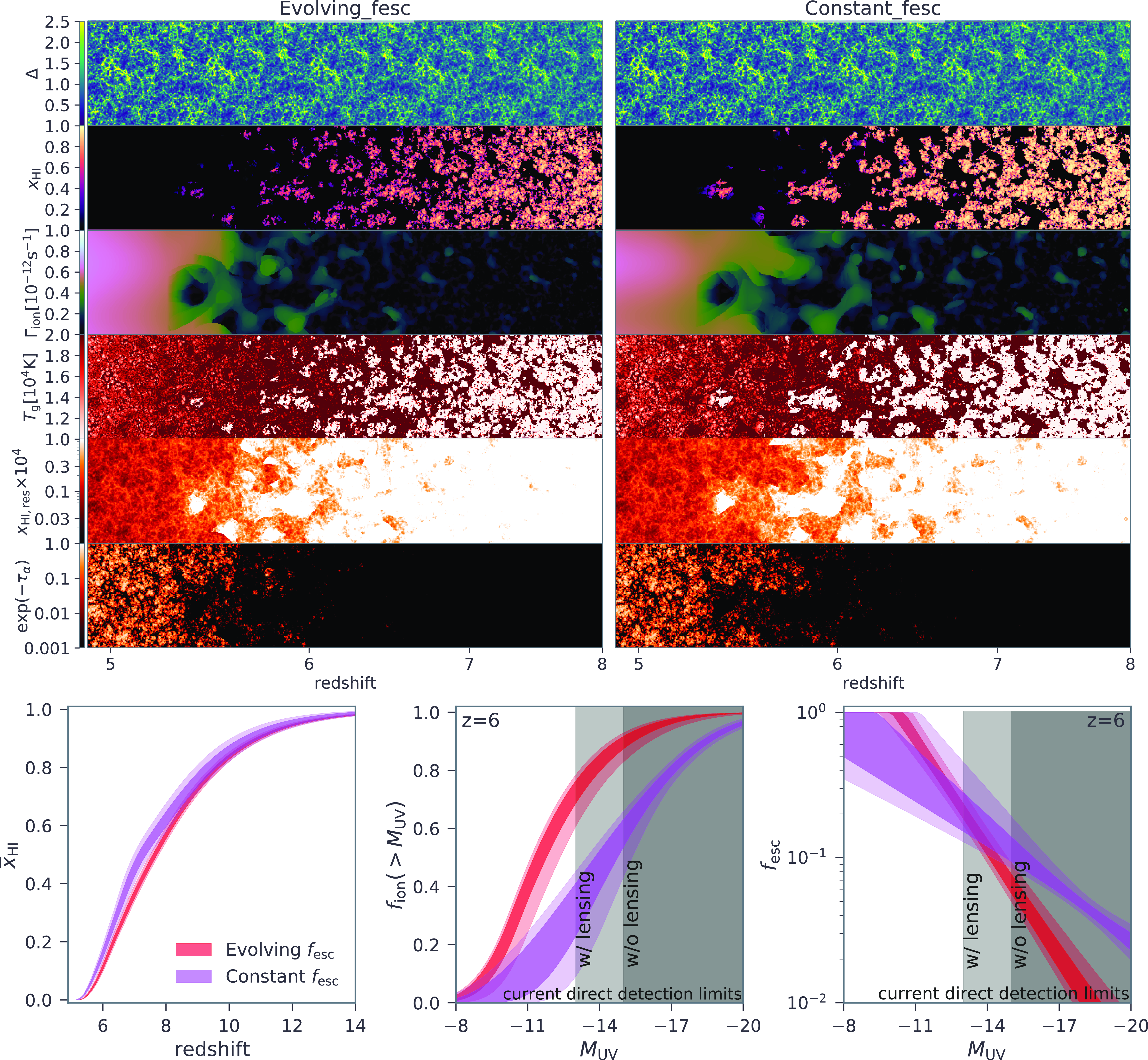
Figure 11.
Upper panels: lightcones of MAP models from $\texttt{Evolving_f}_\texttt{esc}$
and
$\texttt{Evolving_f}_\texttt{esc}$
and $\texttt{Constant_f}_\texttt{esc}$
. From top to bottom, the panels correspond to the overdensity (
$\texttt{Constant_f}_\texttt{esc}$
. From top to bottom, the panels correspond to the overdensity ( $\Delta$
), neutral hydrogen fraction (
$\Delta$
), neutral hydrogen fraction ( $x_\textrm{HI}$
), locally-averaged UVB (
$x_\textrm{HI}$
), locally-averaged UVB ( $\Gamma_\textrm{ion}$
), temperature (
$\Gamma_\textrm{ion}$
), temperature ( $T_\textrm{g}$
), residual neutral fraction within the ionised regions (
$T_\textrm{g}$
), residual neutral fraction within the ionised regions ( $x_\textrm{HI,res}$
) and Ly
$x_\textrm{HI,res}$
) and Ly $\alpha$
transmission. Bottom panels: Similar to Figs. 4 and 10 (
$\alpha$
transmission. Bottom panels: Similar to Figs. 4 and 10 ( $z=6$
only) but for comparisons between
$z=6$
only) but for comparisons between $\texttt{Evolving_f}_\texttt{esc}$
and
$\texttt{Evolving_f}_\texttt{esc}$
and $\texttt{Constant_f}_\texttt{esc}$
and showing the 68% and 95% C.Is of their posterior distributions. Although the two models reach qualitatively the same conclusions about the EoR, the fiducial
$\texttt{Constant_f}_\texttt{esc}$
and showing the 68% and 95% C.Is of their posterior distributions. Although the two models reach qualitatively the same conclusions about the EoR, the fiducial $\texttt{Evolving_f}_\texttt{esc}$
model favors an EoR that is driven by ultra-faint galaxies close to the atomic cooling threshold, resulting in a slightly more extended and patchy EoR.
$\texttt{Evolving_f}_\texttt{esc}$
model favors an EoR that is driven by ultra-faint galaxies close to the atomic cooling threshold, resulting in a slightly more extended and patchy EoR.
In the bottom panel of Fig. 10 we show the mean ionizing escape fraction as a function of UV magnitude, at the same three redshifts, $z=$
6, 8, and 11. We see that the data prefer a population-averaged
$z=$
6, 8, and 11. We see that the data prefer a population-averaged $f_\textrm{esc}$
that increases towards faint galaxies. This is consistent with simulations including RAMSES by Kimm & Cen (Reference Kimm and Cen2014), First Billion Years (Paardekooper, Khochfar, & DallaVecchia 2015), Renaissance (Xu et al. Reference Xu, Wise, Norman, Ahn and O’Shea2016) and Cosmic Dawn II (Lewis et al. Reference Lewis2020) while others such as FIRE-II (Ma et al. Reference Ma, Quataert, Wetzel, Hopkins, Faucher-Giguère and Kereš2020), SPHINX(Rosdahl et al. Reference Rosdahl2022), IllustrisTNG (Kostyuk et al. Reference Kostyuk, Nelson, Ciardi, Glatzle and Pillepich2023), THESAN (Yeh et al. Reference Yeh2023), SPICE (Bhagwat et al. Reference Bhagwat, Costa, Ciardi, Pakmor and Garaldi2024) show different trends in their results. As the posterior distribution of
$f_\textrm{esc}$
that increases towards faint galaxies. This is consistent with simulations including RAMSES by Kimm & Cen (Reference Kimm and Cen2014), First Billion Years (Paardekooper, Khochfar, & DallaVecchia 2015), Renaissance (Xu et al. Reference Xu, Wise, Norman, Ahn and O’Shea2016) and Cosmic Dawn II (Lewis et al. Reference Lewis2020) while others such as FIRE-II (Ma et al. Reference Ma, Quataert, Wetzel, Hopkins, Faucher-Giguère and Kereš2020), SPHINX(Rosdahl et al. Reference Rosdahl2022), IllustrisTNG (Kostyuk et al. Reference Kostyuk, Nelson, Ciardi, Glatzle and Pillepich2023), THESAN (Yeh et al. Reference Yeh2023), SPICE (Bhagwat et al. Reference Bhagwat, Costa, Ciardi, Pakmor and Garaldi2024) show different trends in their results. As the posterior distribution of $\beta_\textrm{esc}$
peaks at
$\beta_\textrm{esc}$
peaks at $\sim-1.6$
, the ionizing escape fraction at a given halo mass decreases at earlier times However, as shown in this panel, such a redshift dependence becomes very mild when
$\sim-1.6$
, the ionizing escape fraction at a given halo mass decreases at earlier times However, as shown in this panel, such a redshift dependence becomes very mild when $f_\textrm{esc}$
is plotted against UV magnitude. The fact that such a mild redshift evolution in the ionizing escape fraction is so strongly preferred by the Bayesian evidence (
$f_\textrm{esc}$
is plotted against UV magnitude. The fact that such a mild redshift evolution in the ionizing escape fraction is so strongly preferred by the Bayesian evidence ( $\texttt{Evolving_f}_\texttt{esc}$
vs
$\texttt{Evolving_f}_\texttt{esc}$
vs $\texttt{Constant_f}_\texttt{esc}$
) highlights again the incredible constraining power of the XQR-30+ forest data.
$\texttt{Constant_f}_\texttt{esc}$
) highlights again the incredible constraining power of the XQR-30+ forest data.
5. How do the results depend on our model?
In the previous section we presented constraints on IGM and galaxy properties using the $\texttt{Evolving_f}_\texttt{esc}$
model, which was strongly favored by the data. Here, we explore how our main conclusions are affected by the choice of galaxy model. Specifically, we compare our fiducial model to
$\texttt{Evolving_f}_\texttt{esc}$
model, which was strongly favored by the data. Here, we explore how our main conclusions are affected by the choice of galaxy model. Specifically, we compare our fiducial model to $\texttt{Constant_f}_\texttt{esc}$
where the UV ionizing escape fraction is solely dependent on the host halo mass. If our results remain largely unaffected by the choice of galaxy model, this would increase confidence in their robustness, regardless of their relative Bayesian evidences.
$\texttt{Constant_f}_\texttt{esc}$
where the UV ionizing escape fraction is solely dependent on the host halo mass. If our results remain largely unaffected by the choice of galaxy model, this would increase confidence in their robustness, regardless of their relative Bayesian evidences.
Fig. 11 shows lightcones corresponding to the MAP in both models (upper panels) and their posteriors for the EoR history (bottom left panel), the cumulative contribution to the $z=6$
ionizing background of galaxies below a given UV magnitude (bottom middle panel), and the ionizing escape fraction as a function of UV magnitude (bottom right panel). Note that the inferred
$z=6$
ionizing background of galaxies below a given UV magnitude (bottom middle panel), and the ionizing escape fraction as a function of UV magnitude (bottom right panel). Note that the inferred $\tau_\textrm{eff}$
CDFs look indistinguishable to those shown in Fig. 3. Both models suggest a qualitatively similar conclusion – reionisation finishes at
$\tau_\textrm{eff}$
CDFs look indistinguishable to those shown in Fig. 3. Both models suggest a qualitatively similar conclusion – reionisation finishes at $z\lt5.5$
with the process primarily driven by ionizing photons emitted by faint galaxies. The end (corresponding to
$z\lt5.5$
with the process primarily driven by ionizing photons emitted by faint galaxies. The end (corresponding to $\overline{x}_\textrm{HI} = 0.01$
) and midpoint of reionisation are at
$\overline{x}_\textrm{HI} = 0.01$
) and midpoint of reionisation are at $z=5.33\pm0.03$
and
$z=5.33\pm0.03$
and $z=7.2\pm0.1$
in the
$z=7.2\pm0.1$
in the $\texttt{Constant_f}_\texttt{esc}$
model, respectively, compared to
$\texttt{Constant_f}_\texttt{esc}$
model, respectively, compared to $z=5.44\pm0.02$
and
$z=5.44\pm0.02$
and $z=7.7\pm0.1$
in our fiducial
$z=7.7\pm0.1$
in our fiducial $\texttt{Evolving_f}_\texttt{esc}$
model.
$\texttt{Evolving_f}_\texttt{esc}$
model.
From the bottom panels of Fig. 11 we see that the models differ quantitatively in which galaxies drive reionisation. The $\texttt{Constant_f}_\texttt{esc}$
model prefers the EoR to be driven by slightly brighter galaxies, with half of the ionizing photons being contributed by
$\texttt{Constant_f}_\texttt{esc}$
model prefers the EoR to be driven by slightly brighter galaxies, with half of the ionizing photons being contributed by $M_\textrm{uv} \gtrsim -14$
galaxies (compared to
$M_\textrm{uv} \gtrsim -14$
galaxies (compared to $M_\textrm{uv} \gtrsim -12$
in the fiducial model). This is due to the fact that without the additional flexibility of a time-evolving
$M_\textrm{uv} \gtrsim -12$
in the fiducial model). This is due to the fact that without the additional flexibility of a time-evolving $f_\textrm{esc}$
, the
$f_\textrm{esc}$
, the $\texttt{Constant_f}_\texttt{esc}$
model results in an EoR history that is too rapid compared with what the data prefer. It is a testament to the constraining power of the XQR-30+ data that only a small redshift evolution in the ionizing escape fraction (c.f. bottom panel of Fig. 10) results in a much higher Bayesian evidence for the
$\texttt{Constant_f}_\texttt{esc}$
model results in an EoR history that is too rapid compared with what the data prefer. It is a testament to the constraining power of the XQR-30+ data that only a small redshift evolution in the ionizing escape fraction (c.f. bottom panel of Fig. 10) results in a much higher Bayesian evidence for the $\texttt{Evolving_f}_\texttt{esc}$
model.
$\texttt{Evolving_f}_\texttt{esc}$
model.
6. Conclusions
The Ly $\alpha$
forests observed in the spectra of high-redshift quasars provide critical insight into the final stages of reionisation. In this work, we introduced a novel framework of 21cmFAST that integrates large-scale lightcones of IGM properties and incorporates unresolved sub-grid physics in the Ly
$\alpha$
forests observed in the spectra of high-redshift quasars provide critical insight into the final stages of reionisation. In this work, we introduced a novel framework of 21cmFAST that integrates large-scale lightcones of IGM properties and incorporates unresolved sub-grid physics in the Ly $\alpha$
opacity, calibrated against high-resolution hydrodynamic simulations for missing physics on small scales. By sampling only 7 free parameters that are capable of characterizing the average stellar-to-halo mass relation, UV ionizing escape fraction, duty cycle and timescale of stellar buildup for high-redshift galaxies, we performed Bayesian inference against the latest Ly
$\alpha$
opacity, calibrated against high-resolution hydrodynamic simulations for missing physics on small scales. By sampling only 7 free parameters that are capable of characterizing the average stellar-to-halo mass relation, UV ionizing escape fraction, duty cycle and timescale of stellar buildup for high-redshift galaxies, we performed Bayesian inference against the latest Ly $\alpha$
forest measurement from XQR-30+ complemented by the observed high-redshift galaxy UV LFs and the CMB optical depth. We demonstrated that current data can constrain global IGM properties with percent-level precision.
$\alpha$
forest measurement from XQR-30+ complemented by the observed high-redshift galaxy UV LFs and the CMB optical depth. We demonstrated that current data can constrain global IGM properties with percent-level precision.
One of the key outcomes of our model is the ability to reproduce the large-scale fluctuations in Ly $\alpha$
opacity without requiring a sharp decline in the ionizing emissivity from
$\alpha$
opacity without requiring a sharp decline in the ionizing emissivity from $z\sim7$
to 5.5, a feature that has been invoked by several other models. In particular, our fiducial model finds reionisation occurs at
$z\sim7$
to 5.5, a feature that has been invoked by several other models. In particular, our fiducial model finds reionisation occurs at $z=5.44\pm0.02$
with a midpoint at
$z=5.44\pm0.02$
with a midpoint at $z=7.7\pm0.1$
. The ionizing escape fraction in this model increases towards fainter galaxies, exhibiting only a mild redshift evolution at a fixed UV magnitude. This suggests that half of the ionizing photons responsible for reionisation are sourced by galaxies fainter than
$z=7.7\pm0.1$
. The ionizing escape fraction in this model increases towards fainter galaxies, exhibiting only a mild redshift evolution at a fixed UV magnitude. This suggests that half of the ionizing photons responsible for reionisation are sourced by galaxies fainter than $M_\textrm{UV}\sim-12$
, which lie below the detection threshold of current optical and near-infrared instruments including JWST.
$M_\textrm{UV}\sim-12$
, which lie below the detection threshold of current optical and near-infrared instruments including JWST.
Additionally, we explored an alternative galaxy model that limits the redshift evolution in the ionizing escape fraction, allowing it to only vary with the host halo mass and reducing the number of free parameters to 6. Although this model demonstrates lower Bayesian evidence relative to our fiducial case, the posteriors for the evolution of IGM properties are in qualitative agreement. This lends confidence that our conclusions on the progress of the EoR are robust. The models do differ somewhat on which galaxies were driving reionisation, with the lower evidence model suggesting galaxies fainter than $M_\textrm{UV} \sim -14$
provided half the ionizing photon budget (compared to
$M_\textrm{UV} \sim -14$
provided half the ionizing photon budget (compared to $M_\textrm{UV} \sim -12$
for the fiducial model).
$M_\textrm{UV} \sim -12$
for the fiducial model).
Future observations both in the Ly $\alpha$
forest and in direct galaxy surveys, will be crucial to further refining these models and improving our understanding of which galaxies drive reionisation as well as the early stages of the EoR (where we currently only have indirect constraints). Our Bayesian framework, allowing us to connect galaxy properties to IGM evolution in a physically-intuitive manner, represents a significant step forward, offering a versatile and efficient tool for interpreting upcoming observational data.
$\alpha$
forest and in direct galaxy surveys, will be crucial to further refining these models and improving our understanding of which galaxies drive reionisation as well as the early stages of the EoR (where we currently only have indirect constraints). Our Bayesian framework, allowing us to connect galaxy properties to IGM evolution in a physically-intuitive manner, represents a significant step forward, offering a versatile and efficient tool for interpreting upcoming observational data.
Acknowledgement
The authors gratefully acknowledge the HPC RIVR consortium and EuroHPC JU for funding this research by providing computing resources of the HPC system Vega at the Institute of Information Science (project EHPC-REG-2022R02-213). This work also made use of OzSTAR and Gadi in Australia. YQ acknowledges HPC resources from the ASTAC Large Programs, the RCS NCI Access scheme. YQ is supported by the ARC Discovery Early Career Researcher Award (DECRA) through fellowship #DE240101129. Parts of this research were supported by the Australian Research Council Centre of Excellence for All Sky Astrophysics in 3 Dimensions (ASTRO 3D), through project no. CE170100013. A.M. acknowledges support from the Ministry of Universities and Research (MUR) through the PRIN project ‘Optimal inference from radio images of the epoch of reionisation’, the PNRR project ‘Centro Nazionale di Ricerca in High Performance Computing, Big Data e Quantum Computing’, and the PRO3 Scuole Programme ‘DS4ASTRO’. VD acknowledges financial support from the Bando Ricerca Fondamentale INAF 2022 Large Grant ‘XQR-30’. MGH has been supported by STFC consolidated grants ST/N000927/1 and ST/S000623/1.
Data availability statement
The data underlying this article will be shared on reasonable request to the corresponding author.
Appendix A. Detailed posteriors
Fig. A1 presents the marginalised 1D and 2D posterior distributions of the model parameters of various models discussed in the work, including the fiducial model $\texttt{Evolving_f}_\texttt{esc}$
, and this model without XQR-30+ data, as well as
$\texttt{Evolving_f}_\texttt{esc}$
, and this model without XQR-30+ data, as well as $\texttt{Constant_f}_\texttt{esc}$
. Tables A1 and A2 list the inferred neutral fraction, UVB, MFP and galaxy UV LFs for the MAP model and [16, 84]th percentiles of
$\texttt{Constant_f}_\texttt{esc}$
. Tables A1 and A2 list the inferred neutral fraction, UVB, MFP and galaxy UV LFs for the MAP model and [16, 84]th percentiles of $\texttt{Evolving_f}_\texttt{esc}$
.
$\texttt{Evolving_f}_\texttt{esc}$
.
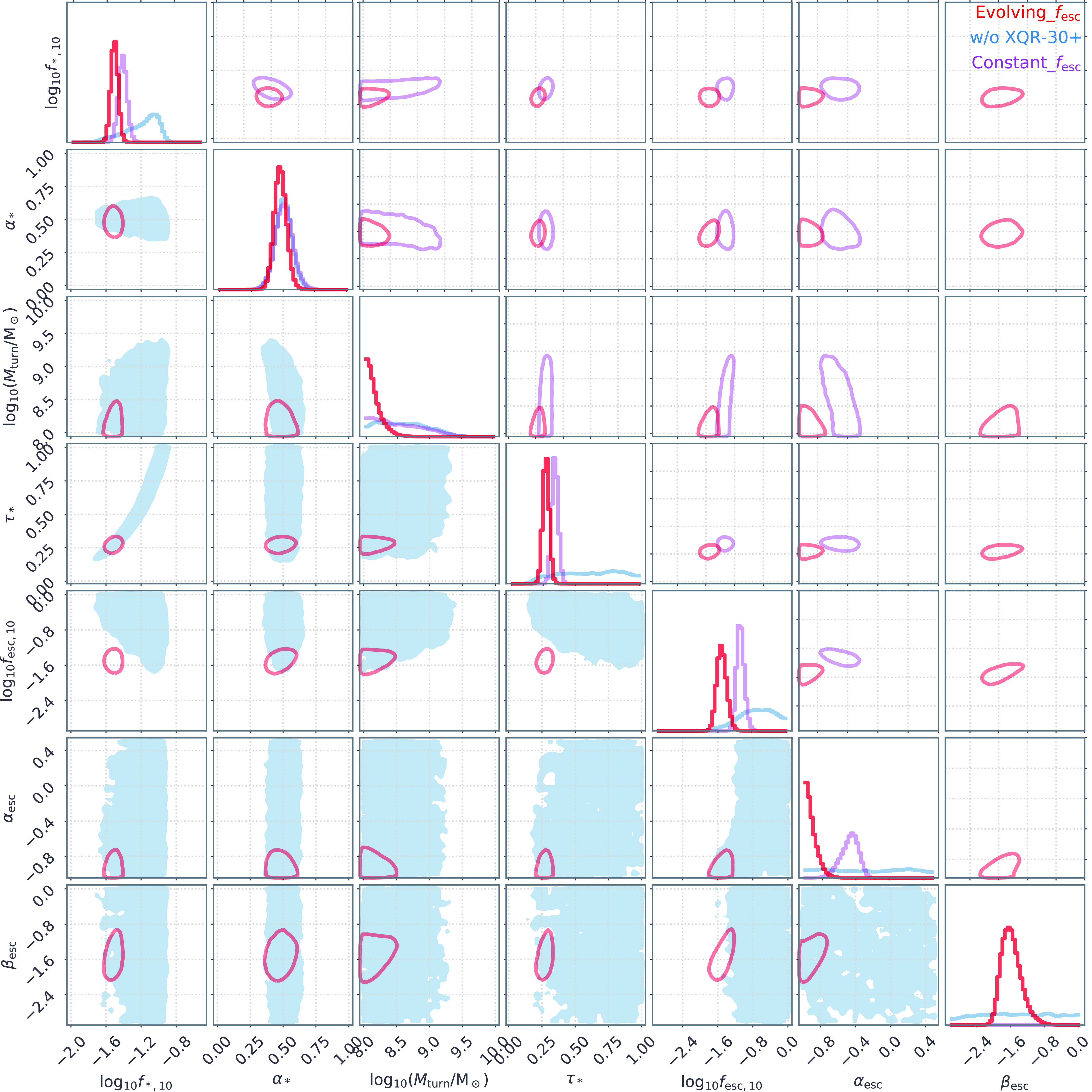
Figure A1. Marginalised 1D and 2D posterior distributions of model parameters from the fiducial model $\texttt{Evolving_f}_\texttt{esc}$
(red), and this model without XQR-30+ (blue) as well as
$\texttt{Evolving_f}_\texttt{esc}$
(red), and this model without XQR-30+ (blue) as well as $\texttt{Constant_f}_\texttt{esc}$
(purple). Regions inside the curves or indicated in shades represent the 95th percentiles.
$\texttt{Constant_f}_\texttt{esc}$
(purple). Regions inside the curves or indicated in shades represent the 95th percentiles.
Table A1. The inferred neutral fraction, photoionzing rate and MFP for the MAP model and the [16, 84]th percentiles (see also Figs. 4 and 5).
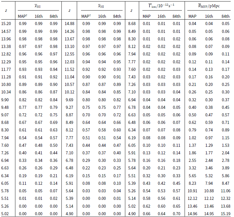
 $^{\dagger}$
The inferred MAP
$^{\dagger}$
The inferred MAP $\overline{x}_\textrm{HI}(z)$
can be represented by a simple ratio of two polynomials with high accuracy (
$\overline{x}_\textrm{HI}(z)$
can be represented by a simple ratio of two polynomials with high accuracy ( $|\Delta \overline{x}_\textrm{HI}|\lt0.01$
) using the following functional form:
$|\Delta \overline{x}_\textrm{HI}|\lt0.01$
) using the following functional form: $x_\textrm{HI}(z) = (292.6 - 105.47z + 7.824z^2 +0.312z^3) / (\def\negativespace{}-24.3 + 22.9z-4.96z^2 + 0.694z^3)$
.
$x_\textrm{HI}(z) = (292.6 - 105.47z + 7.824z^2 +0.312z^3) / (\def\negativespace{}-24.3 + 22.9z-4.96z^2 + 0.694z^3)$
.
Table A2. The inferred galaxy UV luminosity functions for the MAP model and the [16, 84]th percentiles (see also Fig. 9).
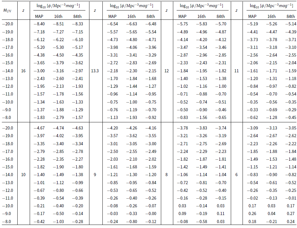


 Open access