


Preface
The following set of articles describe in detail the science goals of the future Space Infrared Telescope for Cosmology and Astrophysics (SPICA). The SPICA satellite will employ a 2.5-m telescope, actively cooled to below 8 K, and a suite of mid- to far-infrared spectrometers and photometric cameras, equipped with state-of-the-art detectors. In particular, the SPICA Far Infrared Instrument (SAFARI) will be a grating spectrograph with low (R  $=$ 300) and medium (R $=$ 3 000–11 000) resolution observing modes instantaneously covering the 35–230 $\mu$m wavelength range. The SPICA Mid-Infrared Instrument (SMI) will have three operating modes: a large field-of-view (12 arcmin $\times$10 arcmin) low-resolution 17–36 $\mu$m spectroscopic (R $=$ 50–120) and photometric camera at 34 $\mu$m, a medium resolution (R $=$ 2 000) grating spectrometer covering wavelengths of 18–36 $\mu$m and a high-resolution echelle module (R $=$ 28 000) for the 12–18 $\mu$m domain. A large field-of-view (160 arcsec $\times$160 arcsec),Footnote a three-channel (100, 200, and 350 $\mu$m) polarimetric camera (B-BOPFootnote b) will also be part of the instrument complement. These articles will focus on some of the major scientific questions that the SPICA mission aims to address; more details about the mission and instruments can be found in Roelfsema et al. (Reference Roelfsema2018).
1. Introduction: SPICA and the nature of cosmic magnetism
Alongside gravity, magnetic fields play a key role in the formation and evolution of a wide range of structures in the Universe, from galaxies to stars and planets. They simultaneously are an actor, an outcome, and a tracer of cosmic evolution. These three facets of cosmic magnetism are intertwined and must be thought of together. On one hand, the role magnetic fields play in the formation of stars and galaxies results from and traces their interplay with gas dynamics. On the other hand, turbulence is central to the dynamo processes that initially amplified cosmic magnetic fields and have since maintained their strength in galaxies across time (Brandenburg & Subramanian Reference Brandenburg and Subramanian2005). A transfer from gas kinetic to magnetic energy inevitably takes place in turbulent cosmic flows, while magnetic fields act on gas dynamics through the Lorentz force. These physical couplings relate cosmic magnetism to structure formation in the Universe across time and scales, and make the observation of magnetic fields a tracer of cosmic evolution, which is today yet to be disclosed. Improving our observational understanding of cosmic magnetism on a broad range of physical scales is thus at the heart of the ‘Origins’ big question and is an integral part of one of ESA’s four Grand Science Themes (‘Cosmic Radiation and Magnetism’) as defined by the ESA High-level Science Policy Advisory Committee in 2013.
As often in Astrophysics, our understanding of the Universe is rooted in observations of the very local universe: the Milky Way and nearby galaxies. In the interstellar medium (ISM) of these galaxies, the magnetic energy is observed to be in rough equipartition with the kinetic (e.g., turbulent), radiative, and cosmic ray energies, all on the order of  ${\sim} 1\, {\rm eV\, cm^{-3}} $, suggesting that magnetic fields are a key player in the dynamics of the ISM (e.g., Draine Reference Draine2011). Their exact role in the formation of molecular clouds (MCs) and stellar systems is not well understood, however, and remains highly debated (e.g., Crutcher Reference Crutcher2012). Interstellar magnetic fields also hold the key for making headway on other main issues in Astrophysics, including the dynamics and energetics of the multi-phase ISM, the acceleration and propagation of cosmic rays, and the physics of stellar and back-hole feedback. Altogether, a broad range of science topics call for progress in our understanding of interstellar magnetic fields, which in turn motivates ambitious efforts to obtain relevant data (cf. Boulanger et al. Reference Boulanger2018).
Observations of Galactic polarisation are a highlight and a lasting legacy of the Planck space mission. Spectacular images combining the intensity of dust emission with the texture derived from polarisation data have received world-wide attention and have become part of the general scientific culture (Planck 2015 res. I 2016). Beyond their popular impact, the Planck polarisation maps represented an immense step forward for Galactic Astrophysics (Planck 2018 res. XII 2019). Planck has paved the way for statistical studies of the structure of the Galactic magnetic field and its coupling with interstellar matter and turbulence, in the diffuse ISM and star-forming MCs.
The Space Infrared Telescope for Cosmology and Astrophysics (SPICA) proposed to ESA as an M5 mission concept (Roelfsema et al.Reference Roelfsema2018) provides one of the best opportunities to take the next big leap forward and gain fundamental insight into the role of magnetic fields in structure formation in the cold Universe, thanks to the unprecedented sensitivity, angular resolution, and dynamic range of its far-infrared (far-IR) imaging polarimeter, B-BOP $^2$ (previously called SPICA-POL, for ‘SPICA polarimeter’). The baseline B-BOP instrument will allow simultaneous imaging observations in three bands, 100, 200, and $350\, \mu$m, with an individual pixel ${\rm NEP} < 3 \times 10^{-18}\, {\rm W\, Hz}^{-1/2}$, over an instantaneous field-of-view of ${\sim} 2.7$ arcmin $\times 2.7$ arcmin at resolutions of 9, 18, and 32 arcsec, respectively (Rodriguez et al.Reference Rodriguez, Poglitsch and Aliane2018). Benefiting from a 2.5-m space telescope cooled to ${<} 8\, $K, B-BOP will be 2–3 orders of magnitude more sensitive than current or planned far-IR/submillimeter polarimeters (see Section 2.4 below) and will produce far-IR dust polarisation images at a factor 20–30 higher resolution than the Planck satellite. It will provide wide-field 100–350 $\mu$m polarimetric images in Stokes Q and U of comparable quality (in terms of resolution, signal-to-noise ratio, and both intensity and spatial dynamic ranges) to Herschel images in Stokes I.
The present paper gives an overview of the main science drivers for the B-BOP polarimeter and is complementary to the papers by, e.g., Spinoglio et al. (Reference Spinoglio2017) and van der Tak et al. (Reference van der Tak2018) which discuss the science questions addressed by the other two instruments of SPICA, SMI (Kaneda et al.Reference Kaneda2016), and SAFARI (Roelfsema et al.Reference Roelfsema2014), mainly through highly sensitive spectroscopy. The outline is as follows: Section 2 describes the prime science driver for B-BOP, namely high dynamic range polarimetric mapping of Galactic filamentary structures to unravel the role of magnetic fields in the star formation process. Section 3 introduces the contribution of B-BOP to the statistical characterisation of magnetised interstellar turbulence. Sections 4 and 5 emphasise the importance of B-BOP polarisation observations for our understanding of the physics of protostellar dense cores and high-mass star protoclusters, respectively. Section 6 discusses dust polarisation observations of galaxies, focusing mainly on nearby galaxies. Section 7 describes how multi-wavelength polarimetry with B-BOP can constrain dust models and the physics of dust grain alignment. Finally, Sections 8–10 discuss three topics which, although not among the main drivers of the B-BOP instrument, will significantly benefit from B-BOP observations, namely the study of the origin of cosmic rays and of their interaction with MCs (Section 8), the detection of polarised far-IR dust emission from protoplanetary disks, thereby tracing magnetic fields in the inner layers of the disks (Section 9), and the (non-polarimetric) monitoring of protostars in the far-IR, i.e., close to the peak of their spectral energy distributions (SEDs), to provide direct constraints on the process of episodic protostellar accretion (Section 10). Section 11 concludes the paper.
2. Magnetic fields and star formation in filamentary clouds
Understanding how stars form in the cold ISM of galaxies is central in Astrophysics. Star formation is both one of the main factors that drive the evolution of galaxies on global scales and the process that sets the physical conditions for planet formation on local scales. Star formation is also a complex, multi-scale process, involving a subtle interplay between gravity, turbulence, magnetic fields, and feedback mechanisms. As a consequence, and despite recent progress, the basic questions of what regulates star formation in galaxies and what determines the mass distribution of forming stars (i.e., the stellar initial mass function or IMF) remain two of the most debated problems in Astronomy. Today, a popular school of thought for understanding star formation and these two big questions is the gravo-turbulent paradigm (e.g., Mac Low & Klessen Reference Mac Low and Klessen2004; McKee & Ostriker Reference McKee and Ostriker2007; Padoan et al. Reference Padoan, Federrath, Chabrier, Evans, Johnstone, Jørgensen, McKee, Nordlund and Beuther2014), whereby magnetised supersonic turbulence creates structure and seeds in interstellar clouds, which subsequently grow and collapse under the primary influence of gravity. A variation on this scenario is that of dominant magnetic fields in cloud envelopes, and a turbulence-enhanced ambipolar diffusion leading to gravity-dominated subregions (e.g., Li & Nakamura Reference Li and Nakamura2004; Kudoh & Basu Reference Kudoh and Basu2008).
Moreover, while the global rate of star formation in galaxies and the positions of galaxies in the Schmidt–Kennicutt diagram (e.g., Kennicutt & Evans Reference Kennicutt and Evans2012) are likely controlled by macroscopic phenomena such as cosmic accretion, large-scale feedback, and large-scale turbulence (Sánchez Almeida et al. Reference Sánchez Almeida, Elmegreen, Muñoz-Tuñón and Elmegreen2014), there is some evidence that the star formation efficiency in the dense molecular gas of galaxies is nearly universalFootnote c (e.g., Gao & Solomon Reference Gao and Solomon2004; Lada et al. Reference Lada, Forbrich, Lombardi and Alves2012) and primarily governed by the physics of filamentary cloud fragmentation on much smaller scales (e.g., André et al. Reference André, Di Francesco, Ward-Thompson, Inutsuka, Pudritz, Pineda and Beuther2014; Padoan et al. Reference Padoan, Federrath, Chabrier, Evans, Johnstone, Jørgensen, McKee, Nordlund and Beuther2014). As argued in Sections 2.2 and 2.3 below, magnetic fields are likely a key element of the physics behind the formation and fragmentation of filamentary structures in interstellar clouds.
Often ignored, strong, organised magnetic fields, in rough equipartition with the turbulent and cosmic ray energy densities, have been detected in the ISM of a large number of galaxies out to  $z = 2$ (e.g., Beck Reference Beck2015; Bernet et al. Reference Bernet, Miniati, Lilly, Kronberg and Dessauges-Zavadsky2008). Recent cosmological magneto-hydrodynamic (MHD) simulations of structure formation in the Universe suggest that magnetic-field strengths comparable to those measured in nearby galaxies ( $ \mathbin{\lower.3ex\hbox{$\buildrel<\over
{\smash{\scriptstyle\sim}\vphantom{_x}}$}} 10{\mkern 1mu} \mu $G) can be quickly built up in high-redshift galaxies (in
$ \mathbin{\lower.3ex\hbox{$\buildrel<\over
{\smash{\scriptstyle\sim}\vphantom{_x}}$}} 10{\mkern 1mu} \mu $G) can be quickly built up in high-redshift galaxies (in  ${\ll} 1\,$ Gyr), through the dynamo amplification of initially weak seed fields (e.g., Rieder & Teyssier Reference Rieder and Teyssier2017; Marinacci et al. Reference Marinacci2018). Magnetic fields are, therefore, expected to play a dynamically important role in the formation of giant molecular clouds (GMCs) on kpc scales within galaxies (e.g., Inoue & Inutsuka Reference Inoue and Inutsuka2012) and in the formation of filamentary structures leading to individual star formation on $\sim$1–10 $\,$pc scales within GMCs (e.g., Inutsuka et al. Reference Inutsuka, Inoue, Iwasaki and Hosokawa2015; Inoue et al. Reference Inoue, Hennebelle, Fukui, Matsumoto, Iwasaki and Inutsuka2018, see Section 2.3 below). On dense core ( ${\leq} 0.1\, $pc) scales, the magnetic field and angular momentum of most protostellar systems are likely inherited from the processes of filament formation and fragmentation (cf. Misugi et al. Reference Misugi, Inutsuka and Arzoumanian2019). On even smaller ( ${<} 0.01\, $pc or ${<} 2\, 000\, $au) scales, magnetic fields are essential to solve the angular momentum problem of star formation, generate protostellar outflows, and control the formation of protoplanetary disks (e.g., Pudritz et al. Reference Pudritz, Ouyed, Fendt, Brandenburg and Reipurth2007; Machida, Inutsuka, & Matsumoto Reference Machida, Inutsuka and Matsumoto2008; Li et al. Reference Li, Banerjee, Pudritz, Jørgensen, Shang, Krasnopolsky, Maury and Beuther2014).
In this context, B-BOP will be a unique tool for characterising the morphology of magnetic fields on scales ranging from  ${\sim} 0.01\,$pc to ${\sim} 1\,$kpc in Milky Way-like galaxies. In particular, a key science driver for B-BOP is to clarify the role of magnetic fields in shaping the rich web of filamentary structures pervading the cold ISM, from the low-density striations seen in HI clouds and the outskirts of CO clouds (e.g., Clark, Peek, & Putman Reference Clark, Peek and Putman2014; Kalberla et al. Reference Kalberla, Kerp, Haud, Winkel, Ben Bekhti, Flöer and Lenz2016; Goldsmith et al. Reference Goldsmith, Heyer, Narayanan, Snell, Li and Brunt2008) to the denser molecular filaments within which most prestellar cores and protostars are forming according to Herschel results (see Figure 1 and Section 2.2 below).
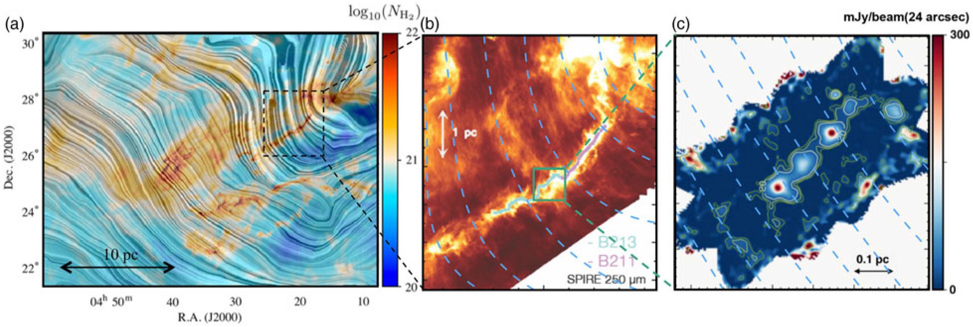
Figure 1. (a) Multi-resolution column-density map of the Taurus MC as derived from a combination of high-resolution (18–36 arcsec half-power beam width (HPBW)) observations from the Herschel Gould Belt survey and low-resolution (5 arcmin half-power beam width - HPBW) Planck data. The superimposed ‘drapery’ pattern traces the magnetic-field orientation projected on the plane of the sky, as inferred from Planck polarisation data at 850  $\mu $m (Planck int. res. XXXV 2016). (b) Herschel/SPIRE 250 $\mu$m dust continuum image of the B211/B213 filament in the Taurus cloud (Palmeirim et al. Reference Palmeirim2013; Marsh et al. Reference Marsh2016). The superimposed blue dashed curves trace the magnetic-field orientation projected on the plane of the sky, as inferred from Planck dust polarisation data at 850 $\mu$m (Planck int. res. XXXV 2016). Note the presence of faint striations oriented roughly perpendicular to the main filament and parallel to the plane-of-sky magnetic field. (c) IRAM/NIKA1 1.2 mm dust continuum image of the central part of the Herschel field shown in (b) (effective HPBW resolution of 20 arcsec), showing a chain of at least four equally spaced dense cores along the B211/B213 filament (from Bracco et al. Reference Bracco2017). B-BOP can image the magnetic-field lines at a factor 30 better resolution than Planck over the entire Taurus cloud [cf. panel (a)], probing scales from ${\sim} 0.01$ to ${>} 10$ pc.
2.1. Dust polarisation observations: a probe of magnetic fields in star-forming clouds
2.1.1. Dust grain alignment
Polarisation of background starlight from dichroic extinction produced by intervening interstellar dust has been known since the late 1940s (Hall Reference Hall1949; Hiltner Reference Hiltner1949). The analysis of the extinction data in polarisation, in particular its variation with wavelength in the visible to near-UV, has allowed major discoveries regarding dust properties, in particular regarding the size distribution of dust. Like the first large-scale total intensity mapping in the far-IR that was provided by the Infrared Astronomical Satellite (IRAS) satellite data, extensive studies of polarised far-IR emission today bring the prospect of a new revolution in our understanding of dust physics. This endeavour includes pioneering observations with ground-based, balloon-borne, and space-borne facilities, such as the very recent all-sky observations by the Planck satellite at  $850\, \mu$m and beyond (e.g., Planck 2018 res. XII 2019). However, polarimetric imaging of polarised dust continuum emission is still in its infancy and amazing improvements are expected in the next decades from instruments such as the Atacama Large Millimeter Array (ALMA) in the submillimeter and B-BOP in the far-IR.
The initial discovery that starlight extinguished by intervening dust is polarised led to the conclusion that dust grains must be somewhat elongated and globally aligned in space in order to produce the observed polarised extinction. While the elongation of dust grains was not unexpected, coherent grain alignment over large spatial scales has been more difficult to explain. A very important constraint has come from recent measurements in emission with, e.g., the Archeops balloon-borne experiment (Benoît et al. Reference Benoît2004) and the Planck satellite (Planck int. res. XIX 2015) which indicated that the polarisation degree of dust emission can be as high as 20% in some regions of the diffuse ISM in the solar neighbourhood. This requires more efficient dust alignment processes than previously anticipated (Planck 2018 res. XII 2019).
The most widely accepted dust grain alignment theories, already alluded to by Hiltner (Reference Hiltner1949), propose that alignment is with respect to the magnetic field that pervades the ISM. Rapidly spinning grains will naturally align their angular momentum with the magnetic-field direction (Purcell Reference Purcell1979; Lazarian & Draine Reference Lazarian and Draine1999), but the mechanism leading to such rapid spin remains a mystery. The formation of molecular hydrogen at the surface of dust grains could provide the required momentum (Purcell Reference Purcell1979). Today’s leading grain alignment theory is Radiative Alignment Torques (RATs) (Dolginov & Mitrofanov Reference Dolginov and Mitrofanov1976; Draine & Weingartner Reference Draine and Weingartner1996; Lazarian & Hoang Reference Lazarian and Hoang2007; Hoang & Lazarian Reference Hoang and Lazarian2016, and references therein), where supra-thermal spinup of irregularly shaped dust grains results from their irradiation by an anisotropic radiation field (a process experimentally confirmed, see Abbas et al. Reference Abbas2004).
2.1.2. Probing magnetic fields with imaging polarimetry
In the conventional picture that the minor axis of elongated dust grains is aligned with the local direction of the magnetic field, mapping observations of linearly polarised continuum emission at far-IR and submillimeter wavelengths are a powerful tool to measure the morphology and structure of magnetic-field lines in star-forming clouds and dense cores (cf.Matthews et al. Reference Matthews, McPhee, Fissel and Curran2009; Crutcher et al. Reference Crutcher, Nutter, Ward-Thompson and Kirk2004; Crutcher Reference Crutcher2012). A key advantage of this technique is that it images the structure of magnetic fields through an emission process that traces the mass of cold interstellar matter, i.e., the reservoir of gas directly involved in star formation. Indirect estimates of the plane-of-sky magnetic-field strength  $B_{\rm POS}$ can also be obtained using the Davis–Chandrasekhar–Fermi method (Davis Reference Davis1951; Chandrasekhar & Fermi Reference Chandrasekhar and Fermi1953): $B_{\rm POS} = \alpha_{\rm corr}\, \sqrt{4\pi \rho}\, \delta V / \delta \Phi $, where $\rho $ is the gas density (which can be estimated to reasonable accuracy from Herschel column-density maps, especially in the case of resolved filaments and cores—cf. Palmeirim et al. Reference Palmeirim2013; Roy et al. Reference Roy2014), $ \delta V $ is the one-dimensional velocity dispersion (which can be estimated from line observations in an appropriate tracer such as N $_2\textit{H}^+$ for star-forming filaments and dense cores—e.g., André et al. Reference André, Belloche, Motte and Peretto2007; Tafalla & Hacar Reference Tafalla and Hacar2015), $ \delta \Phi $ is the dispersion in polarisation position angles directly measured in a dust polarisation map, and $\alpha_{\rm corr} \approx 0.5 $ is a correction factor obtained through numerical simulations (cf. Ostriker, Stone, & Gammie Reference Ostriker, Stone and Gammie2001). Large-scale maps that resolve the above quantities over a large dynamic range of densities can be used to estimate the mass-to-flux ratio in different parts of a MC. This can test the idea that cloud envelopes may be magnetically supported and have a subcritical mass-to-flux ratio (Mouschovias & Ciolek Reference Mouschovias, Ciolek, Lada and Kylafis1999; Shu et al. Reference Shu, Allen, Shang, Ostriker, Li, Lada and Kylafis1999). Recent applications of the Davis–Chandrasekhar–Fermi method using SCUBA2-POL 850 $\mu$m data taken as part of the BISTRO survey (Ward-Thompson et al. Reference Ward-Thompson2017) towards dusty molecular clumps in the Orion and Ophiuchus clouds are presented in Pattle et al. (Reference Pattle2017), Kwon et al. (Reference Kwon2018), and Soam et al. (Reference Soam2018). Refined estimates of both the mean and the turbulent component of $B_{\rm POS}$ can be derived from an analysis of the second-order angular structure function (or angular dispersion function) of observed polarisation position angles $<\Delta\Phi^2 (l)> = \frac{1}{N(l)} \Sigma [\Phi (r) - \Phi (r+l)]^2 $ (Hildebrand et al. Reference Hildebrand, Kirby, Dotson, Houde and Vaillancourt2009; Houde et al. Reference Houde, Vaillancourt, Hildebrand, Chitsazzadeh and Kirby2009). Alternatively, in localised regions where gravity dominates over MHD turbulence, the polarisation-intensity gradient method can be used to obtain maps of the local magnetic-field strength from maps of the misalignment angle, $\delta $, between the local magnetic field (estimated from observed polarisation position angles) and the local column-density gradient (estimated from maps of total dust emission). Indeed, such $\delta $ maps provide information on the local ratio between the magnetic-field tension force and the gravitational force (Koch, Tang, & Ho Reference Koch, Tang and Ho2012; Koch et al. Reference Koch2014). Additionally, the paradigm of Alfvénic turbulence can be tested in dense regions where gravity dominates, in which the observed angular dispersion, $\Delta \Phi$, is expected to decrease in amplitude towards the center of dense cores, where $\delta V$ also decreases (Auddy et al. Reference Auddy, Myers, Basu, Harju, Pineda and Friesen2019).
Because the typical degree of polarised dust continuum emission is low ( $\sim \, $2%–5%—e.g., Matthews et al. Reference Matthews, McPhee, Fissel and Curran2009) and the range of relevant column densities spans 3 orders of magnitude from equivalent visual extinctionsFootnote d $A_V \sim 0.1$ in the atomic medium to $A_V > 100$ in the densest molecular filaments/cores, a systematic dust polarisation study of the rich filamentary networks pervading nearby interstellar clouds and their connection to star formation requires a large improvement in sensitivity, mapping speed, and dynamic range over existing far-IR/submillimeter polarimeters. A big improvement in polarimetric mapping speed is also needed for statistical reasons. As only the plane-of-sky component of the magnetic field is directly accessible to dust continuum polarimetry, a large number of systems must be imaged in various Galactic environments before physically meaningful conclusions can be drawn statistically on the role of magnetic fields. As shown in Section 2.4 below, the required step forward in performance can be uniquely provided by a large, cryogenically cooled space-borne telescope such as SPICA, which can do in far-IR polarimetric imaging what Herschel achieved in total-power continuum imaging.
2.2. Insights from Herschel and Planck: a filamentary paradigm for star formation?
The Herschel mission has led to spectacular advances in our knowledge of the texture of the cold ISM and its link with star formation. While interstellar clouds have been known to be filamentary for a long time (e.g., Schneider & Elmegreen Reference Schneider and Elmegreen1979; Bally et al. Reference Bally, Langer, Stark and Wilson1987; Myers Reference Myers2009, and references therein), Herschel imaging surveys have established the ubiquity of filaments on almost all length scales (approximately  $0.5\,$– $100\,$pc) in the MCs of the Galaxy and shown that this filamentary structure likely plays a key role in the star formation process (e.g., André et al. Reference André2010; Henning et al. Reference Henning, Linz, Krause, Ragan, Beuther, Launhardt, Nielbock and Vasyunina2010; Molinari et al. Reference Molinari2010; Hill et al. Reference Hill2011; Schisano et al. Reference Schisano2014; Wang et al. Reference Wang, Testi, Ginsburg, Walmsley, Molinari and Schisano2015).
The interstellar filamentary structures detected with Herschel span broad ranges in length, central column density, and mass per unit length (e.g., Schisano et al. Reference Schisano2014; Arzoumanian et al. Reference Arzoumanian2019). In contrast, detailed analysis of the radial column-density profiles indicates that, at least in the nearby MCs of the Gould Belt, Herschel filaments are characterised by a narrow distribution of inner widths with a typical value of  ${\sim} 0.1$ pc and a dispersion of less than a factor of 2, when the data are averaged over the filament crests (Arzoumanian et al. Reference Arzoumanian2011, Reference Arzoumanian2019). Independent studies of filament widths in nearby clouds have generally confirmed this result when using submillimeter continuum data (e.g., Koch &Rosolowsky Reference Koch and Rosolowsky2015; Salji et al. Reference Salji2015; Rivera-Ingraham et al. Reference Rivera-Ingraham2016), even if factor of ${\sim}$2–4 variations around the mean inner width of $\sim 0.1\,$pc has been found along the main axis of a given filament (e.g., Juvela et al. Reference Juvela2012; Ysard et al. Reference Ysard2013). Measurements of filament widths obtained in molecular line tracers (e.g., Pineda et al. Reference Pineda, Goodman, Arce, Caselli, Longmore and Corder2011; Fernández-López et al. Reference Fernández-López2014; Panopoulou et al. Reference Panopoulou, Tassis, Goldsmith and Heyer2014; Hacar et al. Reference Hacar, Tafalla, Forbrich, Alves, Meingast, Grossschedl and Teixeira2018) have been less consistent with the Herschel dust continuum results of Arzoumanian et al. (Reference Arzoumanian2011, Reference Arzoumanian2019), but this can be attributed to the lower dynamic range achieved by observations in any given molecular line tracer. Panopoulou et al. (Reference Panopoulou, Psaradaki, Skalidis, Tassis and Andrews2017) pointed out an apparent contradiction between the existence of a characteristic filament width and the essentially scale-free nature of the power spectrum of interstellar cloud images (well described by a single power law from ${\sim} 0.01$ to ${\sim} 50\,$pc—Miville-Deschênes et al. Reference Miville-Deschênes2010, Reference Miville-Deschênes, Duc, Marleau, Cuillandre, Didelon, Gwyn and Karabal2016), but Roy et al. (Reference Roy2019) showed that there is no contradiction given the only modest area filling factors ( $ \mathbin{\lower.3ex\hbox{$\buildrel<\over {\smash{\scriptstyle\sim}\vphantom{_x}}$}} 10{\mkern 1mu} $) and column-density contrasts ( ${\leq} 100 $ in most cases) derived by Arzoumanian et al. (Reference Arzoumanian2019) for the filaments seen in Herschel images. While further high-resolution submillimeter continuum studies would be required to investigate whether the same result holds beyond the Gould Belt, the median inner width of ${\sim} 0.1\,$pc measured with Herschel appears to reflect the presence of a true common scale in the filamentary structure of nearby interstellar clouds. If confirmed, this result may have far-reaching consequences as it introduces a characteristic scale in a system generally thought to be chaotic and turbulent (i.e., largely scale-free—cf. Guszejnov, Hopkins, & Grudić Reference Guszejnov, Hopkins and Grudić2018). It may thus present a severe challenge in any attempt to interpret all ISM observations in terms of scale-free processes.
Another major result from Herschel studies of nearby clouds is that most ( ${>}75 $) prestellar cores and protostars are found to lie in dense, ‘supercritical’ filaments above a critical threshold $\sim 16\, {\rm M}_\odot $/pc in mass per unit length, equivalent to a critical threshold $\sim 160\, {\rm M}_\odot $/pc $^2$ ( $A_V \sim 8)$ in column density or $n_{{\rm H}_2} \sim 2 \times 10^4\, {\rm cm}^{-3} $ in volume density (André et al. Reference André2010; Könyves et al. Reference Könyves2015; Marsh et al. Reference Marsh2016). A similar column-density threshold for the formation of prestellar cores (at $A_V \sim \, $5–10) had been suggested earlier based on ground-based millimeter and submillimeter studies (e.g., Onishi et al. Reference Onishi, Mizuno, Kawamura, Ogawa and Fukui1998; Johnstone, Di Francesco, & Kirk Reference Johnstone, Di Francesco and Kirk2004; Kirk, Johnstone, & Di Francesco Reference Kirk, Johnstone and Di Francesco2006), but without clear connection to filaments. Interestingly, a comparable threshold in extinction (at $A_V \sim \, $8) has also been observed in the spatial distribution of young stellar objects (YSOs) with Spitzer (e.g., Heiderman et al. Reference Heiderman, Evans, Allen, Huard and Heyer2010; Lada, Lombardi, & Alves Reference Lada, Lombardi and Alves2010; Evans, Heiderman, & Vutisalchavakul Reference Evans, Heiderman and Vutisalchavakul2014).
Overall, the Herschel results support a filamentary paradigm for star formation in two main steps (e.g., André et al. Reference André, Di Francesco, Ward-Thompson, Inutsuka, Pudritz, Pineda and Beuther2014; Inutsuka et al. Reference Inutsuka, Inoue, Iwasaki and Hosokawa2015): First, multiple large-scale compressions of interstellar material in supersonic turbulent MHD flows generate a cobweb of  ${\sim} 0.1$ pc-wide filaments in the cold ISM; second, the densest filaments fragment into prestellar cores (and subsequently protostars) by gravitational instability above the critical mass per unit length $ M_{\rm line,crit} = 2\, c_s^2/G$ of nearly isothermal, cylinder-like filaments (see Figure 1), where $c_s$ is the sound speed and G the gravitational constant. This paradigm differs from the classical gravo-turbulent picture in that it relies on the unique features of filamentary geometry, such as the existence of a critical line mass for nearly isothermal filaments (e.g., Inutsuka & Miyama Reference Inutsuka and Miyama1997, and references therein). The validity and details of the filamentary paradigm are strongly debated, however, and many issues remain open. For instance, according to some numerical simulations, the above two steps may not occur consecutively but simultaneously, in the sense that both filamentary structures and dense cores may grow in mass at the same time (e.g., Gómez & Vázquez-Semadeni Reference Gómez and Vázquez-Semadeni2014; Chen & Ostriker Reference Chen and Ostriker2015). The physical origin of the typical ${\sim} 0.1\,$pc inner width of molecular filaments is also poorly understood and remains a challenge for numerical models (e.g., Padoan et al. Reference Padoan, Juvela, Goodman and Nordlund2001; Hennebelle Reference Hennebelle2013; Smith, Glover, & Klessen Reference Smith, Glover and Klessen2014; Federrath Reference Federrath2016; Ntormousi et al. Reference Ntormousi, Hennebelle, André and Masson2016). Auddy et al. (Reference Auddy, Basu and Kudoh2016) point out that magnetised filaments may actually be ribbon-like and quasi-equilibrium structures supported by the magnetic field, and therefore, not have cylindrical symmetry. Regardless of any particular scenario, there is nevertheless little doubt after Herschel results that dense molecular filaments represent an integral part of the initial conditions of the bulk of star formation in our Galaxy.
As molecular filaments are known to be present in the Large Magellanic Cloud (LMC—Fukui et al. Reference Fukui2015), the proposed filamentary paradigm may have implications on galaxy-wide scales. Assuming that all filaments have similar inner widths, it has been argued that they may help to regulate the star formation efficiency in dense molecular gas (André et al. Reference André, Di Francesco, Ward-Thompson, Inutsuka, Pudritz, Pineda and Beuther2014), and that they may be responsible for a quasi-universal star formation law in the dense molecular ISM of galaxies (cf. Lada et al. Reference Lada, Forbrich, Lombardi and Alves2012; Shimajiri et al. Reference Shimajiri2017), with possible variations in extreme environments such as the CMZ (Longmore et al. Reference Longmore2013; Federrath et al. Reference Federrath2016).
In parallel, the Planck mission has led to major advances in our knowledge of the geometry of the magnetic field on large scales in the Galactic ISM. The first all-sky maps of dust polarisation provided by Planck at 850  $\, \mu$m have revealed a very organised magnetic-field structure on $ \mathbin{\lower.3ex\hbox{$\buildrel>\over {\smash{\scriptstyle\sim}\vphantom{_x}}$}} $1–10 pc scales in Galactic interstellar clouds (Planck int. res. XXXV 2016, see Figure 1a). The large-scale magnetic field tends to be aligned with low-density filamentary structures with subcritical line masses such as striations (see Figure 1b) and perpendicular to dense star-forming filaments with supercritical line masses (Planck int. res. XXXII 2016; Planck int. res. XXXV 2016, see Figure 1b and c), a trend also seen in optical and near-IR polarisation observations (Chapman et al. Reference Chapman, Goldsmith, Pineda, Clemens, Li and Krcčo2011; Palmeirim et al. Reference Palmeirim2013; Panopoulou, Psaradaki, & Tassis Reference Panopoulou, Psaradaki and Tassis2016; Soler et al. Reference Soler2016). There is also a hint from Planck polarisation observations of the nearest clouds that the direction of the magnetic field may change within dense filaments from nearly perpendicular in the ambient cloud to more parallel in the filament interior (cf. Planck int. res. XXXIII 2016). These findings suggest that magnetic fields are dynamically important and play a key role in the formation and evolution of filamentary structures in interstellar clouds, supporting the view that dense molecular filaments form by accumulation of interstellar matter along field lines.
The low resolution of Planck polarisation data (10 arcmin at best or 0.4 pc in nearby clouds) is, however, insufficient to probe the organisation of field lines in the  ${\sim} 0.1\,$pc interior of filaments, corresponding both to the characteristic transverse scale of filaments (Arzoumanian et al. Reference Andersson, Pintado, Potter, Straižys and Charcos-Llorens2011, Reference Arzoumanian2019) and to the scale at which fragmentation into prestellar cores occurs (cf. Tafalla & Hacar Reference Tafalla and Hacar2015). Consequently, the geometry of the magnetic field within interstellar filaments and its effects on fragmentation and star formation are essentially unknown today.
2.3. Investigating the role of magnetic fields in the formation and evolution of molecular filaments with B-BOP
Improving our understanding of the physics and detailed properties of molecular filaments is of paramount importance as the latter are representative of the initial conditions of star formation in MCs and GMCsFootnote e (see Section 2.2 above). In particular, investigating how dense, ‘supercritical’ molecular filaments can maintain a roughly constant  $\sim$0.1 $\,$pc inner width and fragment into prestellar cores instead of collapsing radially to spindles is crucial to understanding star formation. The topology of magnetic-field lines may be one of the key elements here. For instance, a longitudinal magnetic field can support a filament against radial collapse but not against fragmentation along its main axis, while a perpendicular magnetic field works against fragmentation and increases the critical mass per unit length but cannot prevent the radial collapse of a supercritical filament (e.g., Tomisaka Reference Tomisaka2014; Hanawa, Kudoh, & Tomisaka Reference Hanawa, Kudoh and Tomisaka2017). The actual topology of the field within molecular filaments is likely more complex and may be a combination of these two extreme configurations.
One plausible evolutionary scenario, consistent with existing observations, is that star-forming filaments accrete ambient cloud material along field lines through a network of magnetically dominated striations (e.g., Palmeirim et al. Reference Palmeirim2013; Cox et al. Reference Cox2016; Shimajiri et al. Reference Shimajiri, André, Palmeirim, Arzoumanian, Bracco, Könyves, Ntormousi and Ladjelate2019, see also Figures 1b and 2a). Accretion-driven MHD waves may then generate a system of velocity-coherent fibres within dense filaments (Hacar et al. Reference Hacar, Tafalla, Kauffmann and Kovács2013, Reference Hacar, Tafalla, Forbrich, Alves, Meingast, Grossschedl and Teixeira2018; Arzoumanian et al. Reference Arzoumanian, André, Peretto and Könyves2013; Hennebelle & André Reference Hennebelle and André2013, cf. Figure 2) and the corresponding organisation of magnetic-field lines may play a central role in accounting for the roughly constant  ${\sim} 0.1\,$pc inner width of star-forming filaments as measured in Herschel observations (cf. Section 2.2). Constraining this process further is key to understanding star formation itself, since filaments with supercritical masses per unit length would otherwise undergo rapid radial contraction with time, effectively preventing fragmentation into prestellar cores and the formation of protostars (e.g., Inutsuka & Miyama Reference Inutsuka and Miyama1997). Information on the geometry of magnetic-field lines within star-forming filaments at $A_V > 8$ is thus crucially needed, and can be obtained through 200–350 $\mu$m dust polarimetric imaging at high angular resolution with B-BOP. Large area coverage and both high angular resolution and high spatial dynamic range are needed to resolve the 0.1 pc scale by a factor ${\sim}$3–10 on one hand and to probe spatial scales from ${>} 10\,$pc in the low-density striations of the ambient cloud (see Figure 1), down to $\sim$0.01–0.03 pc for the fibres of dense filaments (see Figure 2). In nearby Galactic regions (at $d \sim \, $150–500 pc), this corresponds to angular scales from ${>} 5^\circ$ or more down to ${\sim}$20 arcsec or less.
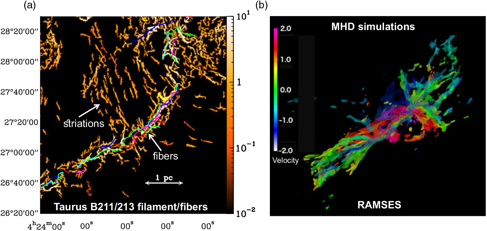
Figure 2. (a) Fine (column) density structure of the B211/B213 filament based on a filtered version of the Herschel 250  $\mu$m image of Palmeirim et al. (Reference Palmeirim2013) using the algorithm getfilaments (Men'shchikov Reference Men’shchikov2013). In this view, all transverse angular scales larger than 72 arcsec (or $\sim 0.05$ pc) were filtered out to enhance the contrast of the small-scale structure. The colour scale is in MJy sr $^{-1}$ at 250 $\mu$m. The coloured curves display the velocity-coherent fibres independently identified by Hacar et al. (Reference Hacar, Tafalla, Kauffmann and Kovács2013) using N $_2\textit{H}^+$/C $^{18}$O observations. (b) MHD simulation of a collapsing/accreting filament performed by E. Ntormousi & P. Hennebelle with the adaptive mesh refinement (AMR) code RAMSES. Line-of-sight velocities (in km/s) after one free-fall time ( $\sim 0.9$ Myr) are coded by colours. For clarity, only the dense gas with $10^4\, {\rm cm}^{-3} < {n_{\rm H_2}} \lt 10^5\, {\rm cm}^{-3} $ is shown. Note the braid-like velocity structure and the morphological similarity with the fibre-like pattern seen in the B211/B213 observations on the left. Thanks to its high resolution and dynamic range, B-BOP can probe, for the first time, the geometry of the magnetic field within the dense system of fibres and the connection with the low-density striations in the ambient cloud.
Low-density striations are remarkably ordered structures in an otherwise chaotic-looking turbulent medium. While the exact physical origin of both low-density striations (Heyer et al. Reference Heyer, Goldsmith, Yıldız, Snell, Falgarone and Pineda2016; Tritsis & Tassis Reference Tritsis and Tassis2016, Reference Tritsis and Tassis2018; Chen et al. Reference Chen, Li, King and Fissel2017) and high-density fibres (e.g., Clarke et al. Reference Clarke, Whitworth, Duarte-Cabral and Hubber2017; Zamora-Avilés, Ballesteros-Paredes, & Hartmann Reference Zamora-Avilés, Ballesteros-Paredes and Hartmann2017) is not well understood and remains highly debated in the literature, there is little doubt that magnetic fields are involved. For instance, Tritsis and Tassis (Reference Tritsis and Tassis2016) modelled striations as density fluctuations associated with magnetosonic waves in the linear regime (the column-density contrast of observed striations does not exceed 25%). These waves are excited as a result of the passage of Alfvén waves, which couple to other MHD modes through phase mixing (see Figure 3, right panel). In contrast, Chen et al. (Reference Chen, Li, King and Fissel2017) proposed that striations do not represent real density fluctuations, but are rather a line-of-sight column-density effect in a corrugated layer forming in the dense post-shock region of an oblique MHD shock. High-resolution polarimetric imaging data would be of great interest to set direct observational constraints and discriminate between these possible models. Specifically, the magnetosonic wave model predicts that a zoo of MHD wave effects should be observable in these regions. One of them, that linear waves in an isolated cloud should establish standing waves (normal modes) imprinted in the striations pattern, has recently been confirmed in the case of the Musca cloud (Tritsis & Tassis Reference Tritsis and Tassis2018). Other such effects include the ‘sausage’ and ‘kink’ modes (see Figure 3, left panel), which are studied extensively in the context of heliophysics (e.g., Nakariakov et al. Reference Nakariakov2016), and which could open a new window to probe the local conditions in MCs (Tritsis et al. Reference Tritsis, Federrath, Schneider and Tassis2018).
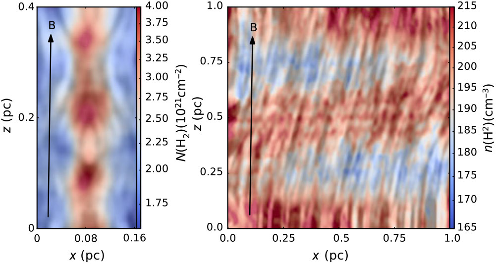
Figure 3. Simulated striations (from Tritsis & Tassis Reference Tritsis and Tassis2016). Right panel: volume density image from the simulations. Left panel: zoomed-in column-density view of a single striation, showing the ‘sausage’ instability setting in, with characteristic imprints in both the magnetic-field and the column-density distribution. In both panels, the drapery pattern traces the magnetic-field lines and the mean direction of the magnetic field is indicated by a black arrow. The passage of Alfvén waves excites magnetosonic modes that create compressions and rarefactions (colourbar) along field lines, giving rise to striations. The simulated data in both panels have been convolved to an effective spatial resolution of 0.012 pc, corresponding to the 18 arcsec HPBW of B-BOP at  $200\, \mu$m.
A first specific objective of B-BOP observations will be to test the hypothesis, tentatively suggested by Planck polarisation results (cf. Planck int. res. XXXIII 2016) that the magnetic field may become nearly parallel to the long axis of star-forming filaments in their dense interiors at scales  ${\lt} 0.1$ pc, due to, e.g., gravitational or turbulent compression (see Figure 4) and/or reorientation of oblique shocks in magnetised colliding flows (Fogerty et al. Reference Fogerty, Carroll-Nellenback, Frank, Heitsch and Pon2017). A change of field orientation inside dense star-forming filaments is also predicted by numerical MHD simulations in which gravity dominates and the magnetic field is dragged by gas flowing along the filament axis (Gómez, Vézquez-Semadeni, & Zamora-Avilés Reference Gómez, Vázquez-Semadeni and Zamora-Avilés2018; Li, Klein, & McKee Reference Li, Klein and McKee2018), as observed in the velocity field of some massive infrared dark filaments (Peretto et al. Reference Peretto2014). An alternative topology for the field lines within dense molecular filaments often advocated in the literature is that of helical magnetic fields wrapping around the filament axis (e.g., Fiege &
Pudritz Reference Fiege and Pudritz2000; Stutz & Gould Reference Stutz and Gould2016; Schleicher & Stutz Reference Schleicher and Stutz2018; Tahani et al. Reference Tahani, Plume, Brown and Kainulainen2018). As significant degeneracies exist between different models because only the plane-of-sky magnetic field is directly accessible to dust polarimetry (cf. Reissl et al. Reference Reissl, Stutz, Brauer, Pellegrini, Schleicher and Klessen2018; Tomisaka Reference Tomisaka2015), discriminating between these various magnetic topologies will require sensitive imaging observations of large samples of molecular filaments for which the distribution of viewing angles may be assumed to be essentially random. One advantage of the model of oblique MHD shocks (e.g., Chen & Ostriker Reference Chen and Ostriker2014; Inoue et al. Reference Inoue, Hennebelle, Fukui, Matsumoto, Iwasaki and Inutsuka2018; Lehmann & Wardle Reference Lehmann and Wardle2016) is that it could potentially explain both how dense filaments maintain a roughly constant
${\lt} 0.1$ pc, due to, e.g., gravitational or turbulent compression (see Figure 4) and/or reorientation of oblique shocks in magnetised colliding flows (Fogerty et al. Reference Fogerty, Carroll-Nellenback, Frank, Heitsch and Pon2017). A change of field orientation inside dense star-forming filaments is also predicted by numerical MHD simulations in which gravity dominates and the magnetic field is dragged by gas flowing along the filament axis (Gómez, Vézquez-Semadeni, & Zamora-Avilés Reference Gómez, Vázquez-Semadeni and Zamora-Avilés2018; Li, Klein, & McKee Reference Li, Klein and McKee2018), as observed in the velocity field of some massive infrared dark filaments (Peretto et al. Reference Peretto2014). An alternative topology for the field lines within dense molecular filaments often advocated in the literature is that of helical magnetic fields wrapping around the filament axis (e.g., Fiege &
Pudritz Reference Fiege and Pudritz2000; Stutz & Gould Reference Stutz and Gould2016; Schleicher & Stutz Reference Schleicher and Stutz2018; Tahani et al. Reference Tahani, Plume, Brown and Kainulainen2018). As significant degeneracies exist between different models because only the plane-of-sky magnetic field is directly accessible to dust polarimetry (cf. Reissl et al. Reference Reissl, Stutz, Brauer, Pellegrini, Schleicher and Klessen2018; Tomisaka Reference Tomisaka2015), discriminating between these various magnetic topologies will require sensitive imaging observations of large samples of molecular filaments for which the distribution of viewing angles may be assumed to be essentially random. One advantage of the model of oblique MHD shocks (e.g., Chen & Ostriker Reference Chen and Ostriker2014; Inoue et al. Reference Inoue, Hennebelle, Fukui, Matsumoto, Iwasaki and Inutsuka2018; Lehmann & Wardle Reference Lehmann and Wardle2016) is that it could potentially explain both how dense filaments maintain a roughly constant  ${\sim} 0.1\,$pc width while evolving (cf. Seifried & Walch Reference Seifried and Walch2015) and why the observed spacing of prestellar cores along the filaments is significantly shorter than the characteristic fragmentation scale of 4 $\, \times$ the filament diameter expected in the case of non-magnetised nearly isothermal gas cylinders (e.g., Inutsuka & Miyama Reference Inutsuka and Miyama1992; Nakamura, Hanawa, & Nakano Reference Nakamura, Hanawa and Nakano1993; Kainulainen et al. Reference Kainulainen, Stutz, Stanke, Abreu-Vicente, Beuther, Henning, Johnston and Megeath2017).

Figure 4. (a) 3D view of a model filament system similar to Taurus B211/3 and associated magnetic-field lines (in blue), with a cylindrical filament (red lines) embedded in a sheet-like background cloud (in light green). In this model, the magnetic field in the ambient cloud is nearly (but not exactly) perpendicular to the filament axis and the axial component is amplified by (gravitational or turbulent) compression in the filament interior. (b) Synthetic polarisation map expected at the  ${\sim}$20 arcsec resolution of B-BOP at 200 $\mu$m for the model filament system shown in (a). SPICA will follow the magnetic field all the way from the background cloud to the central filament. (c) Synthetic polarisation map of the same model filament system at the Planck resolution. Note how Planck data cannot constrain the geometry of the field lines within the central filament.
A second specific objective of B-BOP observations will be to better characterise the transition column density at which a switch occurs between filamentary structures primarily parallel to the magnetic field (at low  $N_{{\rm H}_2}$) and filamentary structures preferentially perpendicular to the magnetic field (at high $N_{{\rm H}_2}$) (see Planck int. res. XXXV 2016, and Section 2.2 above). Based on a detailed analysis of numerical MHD simulations, Soler & Hennebelle (Reference Soler and Hennebelle2017) postulated that this transition column density depends primarily on the strength of the magnetic field in the parent MC, and therefore, constitutes a key observable piece of information. Moreover, Chen, King, and Li (Reference Chen, King and Li2016) showed that, in their colliding flow MHD simulations, the transition occurs where the ambient gas is accelerated gravitationally from sub-Alfvénic to super-Alfvénic speeds. They also concluded that the nature of the transition and the 3D magnetic-field morphology in the super-Alfvénic region can be constrained from the observed polarisation fraction and dispersion of polarisation angles in the plane of the sky, which provides information on the tangledness of the field.
As a practical illustration of what could be achieved with B-BOP, a reference polarimetric imaging survey would map, in Stokes I, Q, U at  $100, 200, 350\, \mu$m, the same ${\sim} 500\,$deg $^2$ area in nearby interstellar clouds imaged by Herschel in Stokes I at 70–500 $\, \mu$m as part of the Gould Belt, HOBYS, and Hi-GAL surveys (André et al. Reference André2010; Motte et al. Reference Motte2010; Molinari et al. Reference Molinari2010). To first order, the gain in sensitivity of B-BOP over SPIRE and PACS on Herschel would compensate for the low degree of polarisation (only a few %) and make it possible to obtain Q and U maps of polarised dust emission with a signal-to-noise ratio similar to the Herschel images in Stokes I. Assuming the B-BOP performance parameters given in Table 1 (see also Table 4 of Roelfsema et al. Reference Roelfsema2018 and Table 1 of Rodriguez et al. Reference Rodriguez, Poglitsch and Aliane2018) and an integration time of ${\sim} 2\,$h per square degree, such a survey would reach a signal-to-noise ratio of 7 in Q, U intensity at both 200 and 350 $\, \mu$m in low column-density areas with $A_V \sim 0.2$ (corresponding to the diffuse, cold ISM), for a typical polarisation fraction of 5% and a typical dust temperature of $T_d \sim 15\,$K. The same survey would reach a signal-to-noise ratio of 5 in Q, U at 100 $\, \mu$m down to $A_V \sim 1$. The entire survey of ${\sim} 500\,$deg $^2$ would require ${\sim} 1\,500\,$h of telescope time, including overheads. It would provide key information on the magnetic-field geometry for thousands of filamentary structures spanning ${\sim} 3$ orders of magnitude in column density from low-density subcritical filaments in the atomic (HI) medium at $A_V \lt 0.5$ to star-forming supercritical filaments in the dense inner parts of MCs at $A_V > 100$.
Table 1 B-BOP performance parameters
a Surface brightness level in I to map Q, U at 5 $\sigma$ over 1 deg $^2$ in 10 h assuming 5% fractional polarisation.
b Assuming  ${\geq} 1$ fractional polarisation.
c The first band of B-BOP has recently been shifted from 100  $\mu$m to 70 $\mu$m.
2.4. Key advantages of B-BOP over other polarimetric facilities
Far-IR/submillimeter polarimetric imaging from space with B-BOP will have unique advantages, especially in terms of spatial dynamic range and surface brightness dynamic range. Studying the multi-scale physics of star formation within molecular filaments requires a spatial dynamic range of  ${\sim} 1\,000$ or more to simultaneously probe scales ${>} 10\,$pc in the parent clouds down to ${\sim} 0.01\,$pc in the interior of star-forming filaments (corresponding to angular scales from ${\sim} 18$ arcsec $\,$to ${>} 5 \,^\circ$ in the nearest MCs—see Figure 1). Such a high spatial dynamic range was routinely achieved with Herschel in non-polarised imaging, but has never been obtained in ground-based submillimeter continuum observations. It will be achieved for the first time with B-BOP in polarised far-IR imaging.
The angular resolution and surface brightness dynamic range of B-BOP will make it possible to resolve 0.1 $\,$pc-wide filaments out to 350 pc and to image a few % polarised dust emission through the entire extent of nearby cloud complexes (cf. Figure 1), from the low-density outer parts of MCs ( ${A_V} \mathbin{\lower.3ex\hbox{$\buildrel<\over {\smash{\scriptstyle\sim}\vphantom{_x}}$}} 0.5$) all the way to the densest filaments and cores ( $A_V > 100$). In comparison, Planck had far too low resolution (10 arcmin at best in polarisation) to probe the magnetic field within dense 0.1 pc-wide filaments or detect faint 0.1 pc-wide striations. Near-IR polarimetry cannot penetrate the dense inner parts of star-forming filaments, and ground-based or air-borne millimeter/submillimeter polarimetric instruments, such as SCUBA2-POL (the polarimeter for the Sub-millimetre Common-User Bolometer Array 2—Friberg et al. Reference Friberg, Bastien, Berry, Savini, Graves and Pattle2016), NIKA2-POL (the polarisation channel for the New IRAM KID Arrays 2—cf. Adam et al. Reference Adam2018), HAWC $+$ (the High-resolution Airborne Wideband Camera-Plus for SOFIA, the Stratospheric Observatory for Infrared Astronomy—Harper et al. Reference Harper2018), or BLAST-TNG (the next generation Balloon-borne Large Aperture Submillimeter Telescope for Polarimetry—Galitzki et al. Reference Galitzki2014), will lack the required sensitivity and dynamic range in both spatial scales and intensity.
More specifically, BLAST-Pol, the Balloon-borne Large Aperture Submillimeter Telescope for Polarimetry operating at 250, 350, and 500  $\mu$m (Fissel et al. Reference Fissel2010, Reference Fissel2016), has only modest resolution (30 arcsec–1 arcmin), sensitivity, and dynamic range. HAWC $+$, the far-infrared camera and polarimeter for SOFIA (Dowell et al. Reference Dowell2010) and BLAST-TNG (cf. Dober et al. Reference Dober2014), both benefit from a larger 2.5-m primary mirror equivalent to that of SPICA, and thus, have comparable angular resolution, but are not cooled, and therefore, are 2–3 orders of magnitude less sensitive (Noise Equivalent Power ${\rm NEP} > 10^{-16}\, {\rm W\, Hz}^{-1/2}$) than B-BOP. Stated another way, the mapping speedFootnote f of B-BOP will be 4–5 orders of magnitude higher than that of HAWC $+$ or BLAST-TNG. Future ground-based submillimeter telescopes on high, dry sites such as CCAT-p (the Cerro Chajnantor Atacama Telescope, prime) and CSST (the Chajnantor Submillimeter Survey Telescope) will benefit from larger aperture sizes (6 and 30 m, respectively) and will thus achieve higher angular resolution than SPICA at 350 $\, \mu$m, but will be limited in sensitivity by the atmospheric background load on the detectors and in spatial dynamic range by the need to remove atmospheric fluctuations. The performance and advantage of B-BOP over other instruments for wide-field dust polarimetric imaging are illustrated in Figure 5.
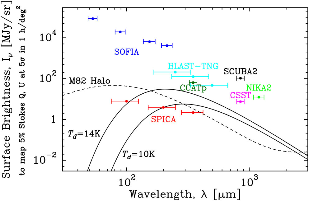
Figure 5. Surface-brightness sensitivity of B-BOP for wide-field polarimetric imaging compared to other existing or planned polarimetric facilities. The total surface-brightness level required to detect polarisation (i.e., Stokes parameters Q, U) with a signal-to-noise ratio of 7 per resolution element (e.g., 9 arcsec pixel at  $200\,\mu $m for B-BOP) when mapping 1 deg $^2$ in 2 h assuming 5% fractional polarisation is plotted as a function of wavelength for each instrument (SOFIA-HAWC $+$, B-BOP, BLAST-TNG, CCAT-p, SCUBA2-POL, CSST, NIKA2-POL). For comparison, the typical surface-brightness level expected in total intensity from the diffuse outer parts of MCs ( $A_V = 1$) is shown for two representative dust temperatures ( $T_d = 10\,$K and $T_d = 14\,$K, assuming simple modified black-body emission with a dust emissivity index $\beta = 2$), as well as the SED of the halo of the nearby galaxy M82 (cf. Galliano, Dwek, & Chanial Reference Galliano, Dwek and Chanial2008; Roussel et al. Reference Roussel2010).
Dust polarimetric imaging with ALMA at  $\lambda \sim \,$0.8–3 $\,$mm will provide excellent sensitivity and resolution, but only on small angular scales (from ${\sim}$0.02 arcsec $\,$ to ${\sim} 20$ arcsec ). Indeed, even with additional observations with ACA (the ALMA Compact Array), the maximum angular scale recoverable by the ALMA interferometer remains smaller than ${\sim}$1 arcmin in total intensity and ${\sim} 20$ arcsec in polarised emission (see ALMA Technical Handbook).Footnote g This implies that ALMA polarimetry is intrinsically insensitive to all angular scales ${>} 20$ arcsec, corresponding to structures larger than 0.015–0.05 $\,$pc in nearby clouds. Using multi-configuration imaging, ALMA can achieve a spatial dynamic range of ${\sim} 1\,000$, comparable to that of Herschel or B-BOP, but only for relatively high surface brightness emission. Because ALMA can only image the sky at high resolution, it is indeed ${\sim}$2–3 orders of magnitude less sensitive to low surface brightness emission than a cooled single-dish space telescope such as SPICA. Expressed in terms of column density, this means that ALMA can only produce polarised dust continuum images of compact objects with ${N_{{{\rm{H}}_2}}} \mathbin{\lower.3ex\hbox{$\buildrel>\over {\smash{\scriptstyle\sim}\vphantom{_x}}$}} {10^{23}}{\mkern 1mu} {\rm{c}}{{\rm{m}}^{ - 2}}$ (such as sub-structure in distant, massive supercritical filaments—see Beuther et al. Reference Beuther2018) at significantly higher resolution ( ${\sim} 1$ arcsec $\,$ or better) than SPICA, while polarimetric imaging of extended, low column-density structures down to ${N_{{{\rm{H}}_2}}} \mathbin{\lower.3ex\hbox{$\buildrel>\over {\smash{\scriptstyle\sim}\vphantom{_x}}$}} 5 \times {10^{20}}{\mkern 1mu} {\rm{c}}{{\rm{m}}^{ - 2}}$ (such as subcritical filaments and striations) will be possible with B-BOP. Furthermore, the small size of the primary beam ( ${\sim}$0.3–1 arcmin at 0.8–3 $\,$mm) makes mosaicing of wide ( ${>} 1\, {\rm deg}^2$) fields impractical and prohibitive with ALMA. In practice, ALMA polarimetric studies of star-forming MCs will provide invaluable insight into the role of magnetic fields within individual protostellar cores/disks and will be very complementary to, but will not compete with, the B-BOP observations discussed here which target the role of magnetic fields in the formation and evolution of filaments on larger scales.
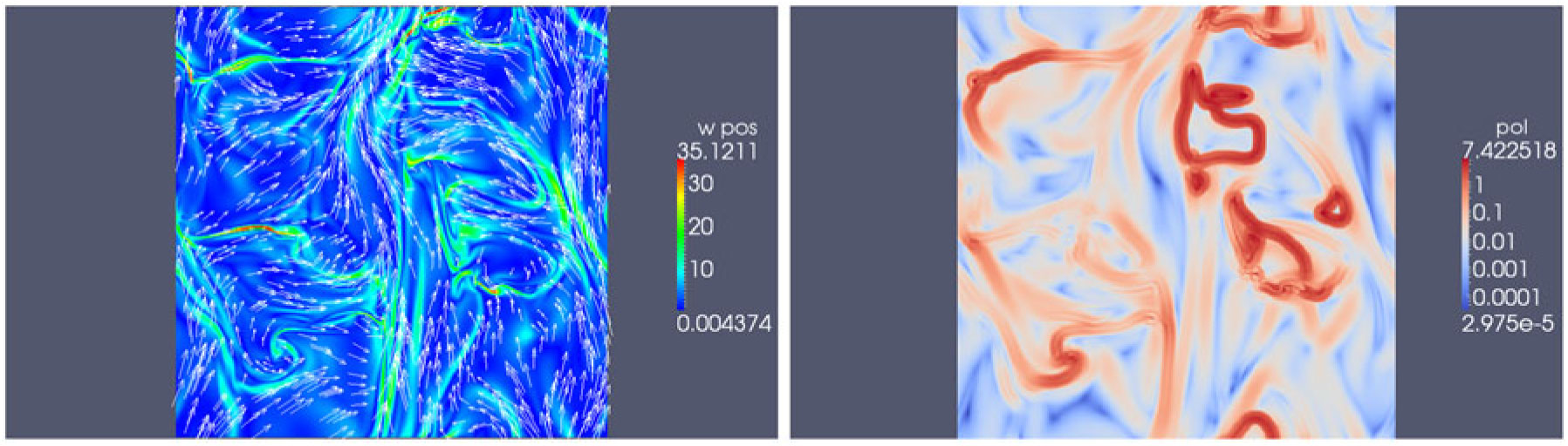
Figure 6. These simulations resolve the dissipation scales of turbulence; they characterise the morphology of magnetic structures formed in magnetised turbulence. For parameters typical of diffuse MCs, the box size is  ${\approx}$1 pc. Left: projections of the vorticity (the modulus in colour) and of the magnetic field (arrows) on the plane of the sky. Right: small-scale increments of the orientation of the plane-of-the-sky component of the magnetic field, a proxy for the dust polarisation angle gradient. Source: Figure adapted from Falgarone, Momferratos, and Lesaffre (Reference Falgarone, Momferratos, Lesaffre, Lazarian, de Gouveia Dal Pino and Melioli2015).
3. The turbulent magnetised ISM
Magnetic fields and turbulence are central to the dynamics and energetics of gas in galactic disks, but also in their halos and possibly in the cosmic web at large. These two intertwined actors of cosmic evolution coupled to gravity drive the formation of coherent structures from the warm and hot tenuous gas phases to the onset of star formation in MCs.
Reaching a statistical description of turbulence in the magnetised ISM is an outstanding challenge, because its extreme characteristics may not be reproduced in laboratory experiments nor in numerical simulations. This challenge is of fundamental importance to Astrophysics, in particular to understand how galaxies and stars form, as well as the chemical evolution of matter in space. This section summarises the contribution we expect B-BOP to bring to this ambitious endeavour.
3.1. Interstellar magnetic fields
Magnetic fields pervade the multi-phase ISM of galaxies. In the Milky Way, and more generally in local universe galaxies, the ordered (mean) and turbulent (random) components of interstellar magnetic fields are comparable and in near equipartition with turbulent kinetic energy (Heiles & Troland Reference Heiles and Troland2005; Beck Reference Beck2015). The galactic dynamo amplification is saturated, but exchanges between gas kinetic and magnetic energy still occur and are of major importance to gas dynamics. Magnetic fields are involved in the driving of turbulence and in the turbulent energy cascade (Subramanian Reference Subramanian2007). The two facets of interstellar turbulence, gas kinematics and magnetic fields, are dynamically so intertwined that they may not be studied independently of each other.
The multiphase magnetised ISM is far too complex to be described by an analytic theory. Our understanding in this research field follows from observations, MHD simulations and phenomenological models. MHD simulations allow us to quantify the non-linear ISM physics but within numerical constraints that limit their scope. They may guide the interpretation observations but alone they do not provide conclusive answers because they are very far from reproducing the high Reynolds ( $R_e$) and magnetic Prandtl numbers ( $P_m$)Footnote h of interstellar turbulence (Kritsuk et al. Reference Kritsuk2011). The fluctuation dynamo and shock waves contribute to produce highly intermittent magnetic fields where the field strength is enhanced in localised magnetic structures. The volume filling factor of these structures decreases for increasing values of the magnetic Reynolds number $R_m = R_e\times P_m$ (Schekochihin et al. Reference Schekochihin, Maron, Cowley and McWilliams2002; Brandenburg & Subramanian Reference Brandenburg and Subramanian2005). The inhomegeneity in the degree of magnetisation of matter associated with intermittency is an essential facet of interstellar turbulence (Falgarone et al. Reference Falgarone, Momferratos, Lesaffre, Lazarian, de Gouveia Dal Pino and Melioli2015; Nixon & Pringle Reference Nixon and Pringle2019), which simulations miss because they are far from reproducing the interstellar values of $R_m$. In this context, to make headway, we must follow an empirical approach where a statistical model of interstellar turbulence is inferred from observations.
3.2. The promise of B-BOP
B-BOP will image dust polarisation with an unprecedented combination of sensitivity and angular resolution, providing a unique data set (Section 2.4) to characterise the magnetic facet of interstellar turbulence. This leap forward will open an immense discovery space, which will revolutionise our understanding of interstellar magnetic fields, and their correlation with matter and gas kinematics.
At  $200\,\mu$m, for the SED of the diffuse ISM(Planck int. res. XVII 2014), the surface brightness sensitivity of B-BOP is 3 orders of magnitude greater than that of the Planck $353\,$ GHz all-sky map for deep imaging (10 h per square degree) and a few 100 times better for faster mapping (2 h per square degree). The analysis of dust polarisation at high Galactic latitude with the Planck data is limited by sensitivity to an effective angular resolution of ${\sim}1^\circ$ in the diffuse ISM and 10 arcmin in MCs where the column density is larger than $10^{22}\,$H cm $^{-2}$ (Planck 2018 res. XII 2019), while B-BOP will map dust polarisation with a factor $\sim $20–70 better resolution at 100–350 $\, \mu$m.
Dust polarisation probes the magnetic-field orientation in dust-containing regions, i.e., mostly in the cold and warm phases of the ISM, which account for the bulk of the gas mass, and hence of the dust mass. These ISM phases comprise the diffuse ISM and star-forming MCs. They account for most of the gas turbulent kinetic energy in galaxies (Hennebelle & Falgarone Reference Hennebelle and Falgarone2012). Thus, among the various means available to map the structure of interstellar magnetic fields, dust polarisation is best suited to trace the dynamical coupling between magnetic fields, turbulence, and gravity in the ISM. This interplay is pivotal to ISM physics and star formation. It is also central to cosmic magnetism because it underlies dynamo processes (Subramanian Reference Subramanian2007).
Observations have so far taught us that magnetic fields are correlated with the structure of matter in both the diffuse ISM and in MCs (Clark et al. Reference Clark, Peek and Putman2014; Planck int. res. XXXII 2016; Planck int. res. XXXV 2016) but this correlation does not fully describe interstellar magnetism. Data must also be used to characterise the intermittent nature of interstellar magnetic fields.
The magnetic structures identified in MHD simulations (Figure 6) may be described as filaments, ribbons or sheets with at least one dimension commensurate with dissipation scales of turbulent and magnetic energy in shocks, current sheets or through ambipolar diffusion (Momferratos et al. Reference Momferratos, Lesaffre, Falgarone and Pineau des Forêts2014; Falgarone et al. Reference Falgarone, Momferratos, Lesaffre, Lazarian, de Gouveia Dal Pino and Melioli2015). While the viscous and Ohmic dissipation scales of turbulence are too small to be resolved by B-BOP, turbulence dissipation due to ion-neutral friction is expected to occur on typical scales between  ${\sim} 0.03$ and ${\sim} 0.3\,$pc (cf. Momferratos et al. Reference Momferratos, Lesaffre, Falgarone and Pineau des Forêts2014), which is well within the reach of B-BOP for matter in the local ISM.
Although dust polarisation does not measure the field strength, the polarisation angle may be used to map these magnetic structures, as illustrated in Figure 6. The figure shows that the largest values of the increment of the polarisation angle,  $\Delta \Phi$, delineate structures that tend to follow those of intense dissipation of turbulent energy. B-BOP will allow us to identify magnetic structures, such as those in Figure 6, even if their transverse size is unresolved because (i) they are highly elongated and (ii) their spatial distribution in the ISM is fractal.
Regions of intermittency in interstellar turbulence correspond to rare events. Their finding requires obtaining large data sets combining brightness sensitivity and angular resolution, as illustrated by the CO observations with the Institut de Radioastronomie Millimétrique (IRAM) 30-m telescope analysed by Hily-Blant, Falgarone, and Pety (Reference Hily-Blant, Falgarone and Pety2008) and Hily-Blant and Falgarone (Reference Hily-Blant and Falgarone2009). B-BOP has the unique capability to extend these pioneering studies of the intermittency of gas kinematics to dust polarisation observations, tracing the structure of magnetic fields (Section 2.1.2), with a comparable angular resolution. B-BOP will also greatly strengthen their statistical significance by covering a total sky area more than 2 orders of magnitude larger.
B-BOP holds promises to reveal a rich array of magnetic structures, characterising the intermittency of interstellar magnetic fields. Planck data, at a much coarser scale, gives a first insight at the expected outcome of the observations illustrated in Figure 7. Magnetic structures will be identified in the data as locations where the probability distributions of the increments of the polarisation angle, and of the Stokes Q/I and U/I ratios, depart from Gaussian distributions. Compared to Planck, B-BOP will only map a small fraction of the sky ( ${\sim} 1$ for nearby MCs and diffuse ISM observed away from the Galactic plane), but it will probe the field structure on much smaller scales (by a factor 30 or more) where the surface density of magnetic structures is expected to be much larger.
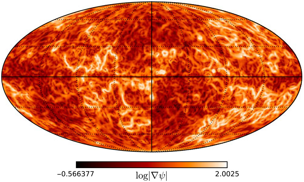
Figure 7. Non-Gaussianity of the magnetic-field structure in the Planck dust polarisation data. This all-sky image, in Galactic coordinates centered on the Galactic center, presents the modulus of the angular polarisation gradient,  $|\nabla{\psi}|$, built from the Planck data at 353 GHz smoothed to 160 arcmin resolution. Source: Figure adapted from Appendix D of Planck 2018 res. XII (2019).
3.3. Observing strategy
B-BOP will considerably expand our ability to map the structure of interstellar magnetic fields. These data will be complementary to a diverse array of polarisation observations of the Galaxy.
Stellar polarisation surveys will be combined with Gaia astrometry (e.g., Tassis et al. Reference Tassis2018) to build 3D maps of the magnetic fields in the Galaxy but with a rather coarse resolution, comparable to that of the density structure of the local ISM in Lallement et al. (Reference Lallement2018).
Synchrotron observations at radio wavelengths with the Square Kilometer Array (SKA) and its precursors will probe the structure of magnetic fields (Dickinson et al. Reference Dickinson2015; Haverkorn et al. Reference Haverkorn2015), in particular, in ionised phases through Faraday rotation (Gaensler et al. Reference Gaensler2011; Zaroubi et al. Reference Zaroubi2015). SKA will also provide Faraday rotation measurements towards  ${\sim} 10^7$ extragalactic sources (Johnston-Hollitt et al. Reference Johnston-Hollitt2015), which will be available for comparison with B-BOP dust polarisation data as illustrated in the pioneering study of Tahani et al. (Reference Tahani, Plume, Brown and Kainulainen2018).
B-BOP will allow us to study interstellar turbulence over an impressive range of physical scales and astrophysical environments from the warm ISM phases to MCs. Observations of nearby galaxies are best suited to probe the driving of turbulence in relation to galaxy dynamics (spiral structure, bars, galaxy interaction, outflows) and stellar feedback as discussed in Section 6. Galactic observations will probe the inertial range of turbulence over 4–5 orders of magnitude from the injection scales ( ${\sim} 100\,$pc– $1\,$kpc) down to $0.01\,$pc. The smallest physical scales will be reached by observing interstellar matter nearest the Sun, away from the Galactic plane: the diffuse ISM at high Galactic latitudes and star-forming MCs in the Gould Belt. These sky regions are best suited for the study of turbulence because the overlap of structures along the line of sight is minimised. The Gould Belt clouds are already part of the filament science case in Section 2. This survey will include star-forming clouds and diffuse clouds representative of the cold neutral medium. Deeper polarimetric imaging of high Galactic latitude fields (10 h per deg $^2$), sampling regions of low gas column density ( $ A_V \sim 0.1$–0.3), will allow us to probe turbulence in the warm ISM phases. These deep imaging observations could potentially share the same fields as those used to carry out a SPICA-SMI cosmological survey. The size of the area that may be mapped to that depth (of order ${\sim} 100\,$deg $^2$) will be optimised with the needs of this survey. Altogether, we estimate that B-BOP will cover a total area of about 500 deg $^2$ away from the Galactic Plane including diffuse ISM fields at high Galactic latitudes, which will be available to study turbulence in diverse interstellar environments. At the angular resolution of B-BOP at $200\,\mu$m, these data correspond to a total of $2 \times 10^7$ polarisation measurements. This number is 20 times larger than the statistics offered by the Planck polarisation data. The gain in angular resolution and sensitivity is so large, that B-BOP will supersede Planck in terms of data statistics, even if the maps used cover only ${\sim} 1$ of the sky.
A wealth of spectroscopic observations of HI and molecular gas species, tracing the gas density, column density and kinematics, will become available before the launch of B-BOP with SKA and its precursors (McClure-Griffiths et al. Reference McClure-Griffiths2015), and the advent of powerful heterodyne arrays on millimeter ground-based telescopes, e.g., the Large Millimeter Telescope and the IRAM 30-m telescope. Furthermore, we will be able to investigate the link between coherent magnetic structures and turbulent energy dissipation observing main ISM cooling lines from H $_2$, C II, and O I with the SPICA mid and far-IR spectrometers SMI and SAFARI. These complementary data from SPICA and ground-based observatories will be combined to characterise the turbulent magnetised ISM statistically. The data analysis will rely on on-going progress in the development of statistical methods (e.g., Makarenko et al. Reference Makarenko, Shukurov, Henderson, Rodrigues, Bushby and Fletcher2018; Allys et al. Reference Allys, Levrier, Zhang, Colling, Regaldo-Saint Blancard, Boulanger, Hennebelle and Mallat2019), which we will use to characterise the structure of interstellar magnetic fields and their correlation with gas density and velocity. This process will converge towards an empirical model of interstellar turbulence, which will be related to ISM physics comparing data and MHD simulations.
4. Magnetic fields in protostellar dense cores
4.1. Current state of the art
In MCs, protostellar dense cores are the ‘seeds’ where the gravitational force proceeds to form stars. Class 0 objects are the youngest known accreting protostars: most of their mass is still in the form of a dense core/envelope ( $M_{\rm env} \gg M_\star $) and this phase is characterised by high accretion rates of gas from the dense core onto the central stellar object, accompanied by ejection of powerful highly collimated flows (André, Ward-Thompson, & Barsony Reference André, Ward-Thompson, Barsony and Mannings2000; Dunham et al. Reference Dunham and Beuther2014).
How many stars can be formed out of a typical MC depends not only on the physical conditions in filamentary structures, but also on the detailed manner the gravitational collapse proceeds within individual protostellar cores (i.e., would it form a single/binary stellar system, one or several low-mass stars or high-mass stars?).
By the end of the protostellar phase, the star has gained most of its final mass: understanding the role of magnetic fields during the protostellar stage is therefore crucial to clarify how they affect some of the most remarkable features of the star formation process, such as the distribution of stellar masses, the stellar multiplicity, or the ability to host planet-forming disks (McKee & Ostriker Reference McKee and Ostriker2007; Li et al. Reference Li, Banerjee, Pudritz, Jørgensen, Shang, Krasnopolsky, Maury and Beuther2014).
The development of numerical MHD models describing the collapse of protostellar cores and the formation of low-mass stars has opened new ways to explore in more details the physical processes responsible for the formation of solar-type stars. MHD models suggest that protostellar collapse proceeding with initially strong and well-aligned magnetic field produces significantly different outcomes than hydrodynamic or weakly magnetised models (Fiedler & Mouschovias Reference Fiedler and Mouschovias1993; Hennebelle & Fromang Reference Hennebelle and Fromang2008; Masson et al. Reference Masson, Chabrier, Hennebelle, Vaytet and Commerçon2016). For example, if the field is strong enough and well coupled to the core material, magnetic braking will regulate the formation of disks and multiple systems during the Class 0 phase. This has been the focus of recent studies (Hennebelle et al. Reference Hennebelle, Commerçon, Chabrier and Marchand2016; Krasnopolsky, Li, & Shang Reference Krasnopolsky, Li and Shang2011; Machida, Inutsuka, & Matsumoto Reference Machida, Inutsuka and Matsumoto2011), because it could potentially explain the low end of the size distribution of protostellar disks (e.g., Maury et al. Reference Maury2010; Segura-Cox et al. Reference Segura-Cox2018; Maury et al. Reference Maury2019).
All protostellar cores are magnetised to some level and current observations suggest that at least in some cases the magnetic field at core scale is remarkably well organised, pointing towards scenarii with strong field even at the high column densities typical of protostellar cores (e.g., IRAS 4A, G31.41, G240.31, NGC 6334, L1157, B335: Girart, Rao, & Marrone Reference Girart, Rao and Marrone2006; Girart et al. Reference Girart, Beltrán, Zhang, Rao and Estalella2009; Qiu et al. Reference Qiu, Zhang, Menten, Liu, Tang and Girart2014; Li et al. Reference Li2015; Stephens et al. Reference Stephens2013; Galametz et al. Reference Galametz2018; Maury et al. Reference Maury2018), while in other cases (e.g., Girart et al. Reference Girart, Frau, Zhang, Koch, Qiu, Tang, Lai and Ho2013; Hull et al. Reference Hull2017; Ching et al. Reference Ching, Lai, Zhang, Girart, Qiu and Liu2017, and Figure 8 for an example in the G14 massive star forming region) the core-scale magnetic field shows very complex morphology. In Figure 8, for instance, it is noteworthy that the northern hub of the G14 region, with a more uniform magnetic field, has a lower level of fragmentation than the southern hub (that shows a more perturbed magnetic field). These observations suggest the field may remain organised at scales where collapse occurs in most solar-type progenitors, and also at least some of the massive cores (Zhang et al. Reference Zhang2014; Beuther et al. Reference Beuther2018). Current results may be biased, however, because present single-dish facilities selectively trace magnetic fields from the brightest regions within star-forming cores (dust polarisation is only detected at the highest column densities, see Figure 8).
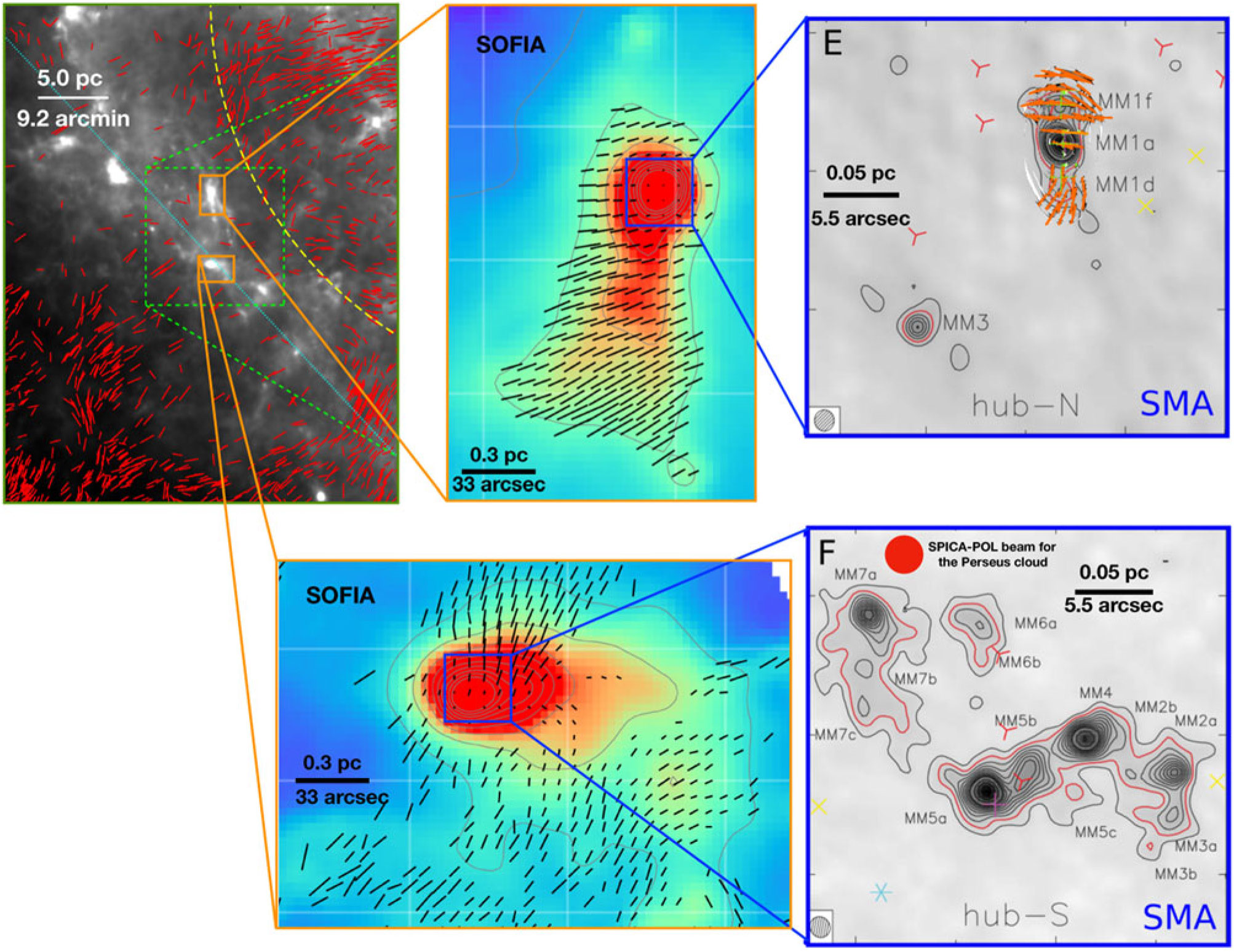
Figure 8. Composite images of the G14.225-0.506 massive star forming region (Busquet et al. Reference Busquet2013, Reference Busquet2016; Santos et al. Reference Santos, Busquet, Franco, Girart and Zhang2016). Top left panel: R band optical polarisation vectors (red segments) overlaid on Herschel 250  $\mu$m image overlapped (from Santos et al. Reference Santos, Busquet, Franco, Girart and Zhang2016). Central panels: SOFIA/HAWC+ 200 $\mu$m images (beam 14 arcsec) of the Northern (top) and Southern (bottom) hubs, with black segments showing the magnetic-field direction (F. Santos, private communication). Right panels: Submillimeter Array (SMA) images of the 1.2 mm emission towards the center of the Northern (top) and Southern (bottom) hubs (Busquet et al. Reference Busquet2016), with orange segments showing the magnetic-field direction (N. Añez-López, private communication).
4.2. Role of magnetic fields in controlling the typical outcome of protostellar collapse
B-BOP can perform statistical studies in unprecedentedly large samples of protostellar cores, testing for example whether the magnetic field in cores is directly inherited from their environment (if the magnetic field in low-density filamentary structures, see Section 2.3, connects to the magnetic field in high-density cores, which is expected in the strong field case), or if the field in cores is disconnected from the local field in the progenitor cloud (weak field case). While the ALMA interferometer can only provide constraints on the magnetic-field topology at the smallest scales (approximately 0.02–20 arcsec, i.e.,  ${\lt}5\,000$ au in Gould Belt clouds), the polarisation capabilities of other facilities probing larger spatial scales (SMA, NIKA2, and HAWC+) are severely sensitivity limited. Accordingly, studies linking cores and filaments can currently be carried out in bright, massive star-forming regions mostly (see Figure 8), and only in a handful of nearby solar-type protostellar cores.
Some indications have been found, in small samples ( ${\lt}20$ objects), that the topology of the magnetic field at core scales may be linked to the distribution of angular momentum in solar-type cores, and hence that the magnetic field may be of paramount importance to set the initial conditions for the formation of protoplanetary disks and multiple systems (see Figure 9 and Galametz et al. Reference Galametz2018; Segura-Cox et al. Reference Segura-Cox2018). An example of the type of studies that B-BOP could extend to the full mass function of protostellar cores in a statistical fashion is shown in Figures 8 and 9: these two figures illustrate the tentative link between the magnetic-field topology at core scale and the disks and multiplicity fraction found within protostellar cores at smaller scale. The magnetic-field properties found with B-BOP at dense core scales can be compared with the protostellar properties observed with interferometers at smaller scales to build correlation diagrams similar to the one shown in Figure 9. In this way, B-BOP observations can test the hypothesis, tentatively suggested by current studies of the brightest protostars, that magnetic fields regulate the formation of disks and multiple systems during the main accretion phase. Observations of large samples of protostars could be carried out thanks to the sensitivity and spatial resolution of B-BOP, which is crucially needed not only to populate diagrams such as Figure 9, but also because only statistics will allow us to solve the degeneracy induced by projection effects intrinsically linked to dust polarisation (tracing only the magnetic-field component in the plane of the sky). Moreover, B-BOP will provide information on the geometry of magnetic-field lines across the full protostellar core mass distribution, probing different behaviours in different mass regimes, and potentially as a function of environment in different star-forming regions.
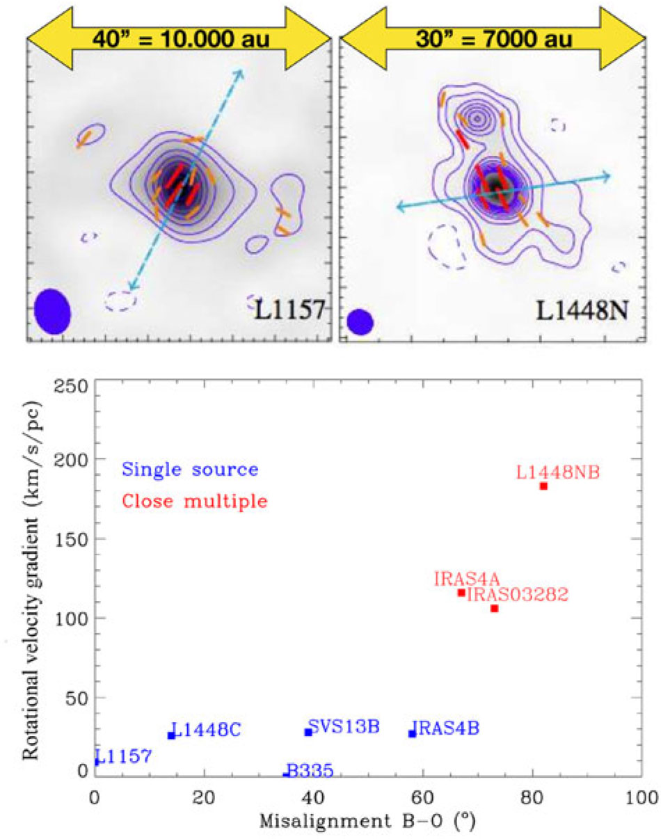
Figure 9. Potential role of the magnetic-field topology at core scales in the formation of disks and multiple systems. Top: magnetic field (red/orange line segments, from dust polarisation observations with the SMA at 850 $\,\mu$m) in two solar-type Class 0 protostellar cores (Galametz et al. Reference Galametz2018). The blue arrows indicate the jet/rotation axis of these cores, aligned with the core-scale magnetic field in L1157 (left), and mostly orthogonal to it in L1448N (right). Bottom: level of core rotation (from kinematic observations at core scales, Yen et al. Reference Yen, Koch, Takakuwa, Ho, Ohashi and Tang2015 and Gaudel et al. Reference Gaudel, Maury and Belloche2019) as a function of the misalignment between the rotation/outflow axis and the magnetic field (observed at core scale with the SMA—Galametz et al. Reference Galametz2018) in a sample of nearby Class 0 sources. There is a hint that large misalignments of the magnetic field at core scales lead to sources with large rotational gradients and multiple systems at smaller scales (red symbols).
The angular resolution and surface brightness dynamic range of B-BOP will make it possible to resolve most  ${\sim}$2 000–20 000 au protostellar cores in nearby star-forming regions out to 250 pc. A wide-field B-BOP survey of all nearby clouds as envisaged in Section 2.3 ( ${\sim} 2\,$h per square degree) will map dust polarisation (fraction $>1\%$) at core scales with signal-to-noise ratio $>7$, in complete populations of $ \mathbin{\lower.3ex\hbox{$\buildrel>\over {\smash{\scriptstyle\sim}\vphantom{_x}}$}} $1 000 protostars (Class 0 and Class I) and their parent cloud/environment, from massive protostellar cores down to the low-mass progenitors of solar-type stars. In contrast, current millimeter/submillimeter polarimetric instruments, such as SCUBA2-POL, NIKA2-POL, SOFIA/HAWC $+$, or BLAST-TNG (cf. Section 2.4) are limited to the subset of the $\sim$50–100 brightest cores, and without the important context provided by the magnetic-field information in the parental clouds.
5. Role of magnetic fields in high-mass star and cluster formation
As mentioned in Section 2.2, supercritical molecular filaments are believed to be the preferred birthplaces of solar-type stars. It is, however, unclear whether the filamentary paradigm—or an extension of it, based on unusually high line masses or levels of turbulence (e.g., Roy et al. Reference Roy2015)—also applies to high-mass star formation and can lead to the quasi-static formation and monolithic collapse of massive prestellar cores, then forming high-mass protostars. The most recent observational results, partly obtained with Herschel, suggest that high-mass stars and stellar clusters form in denser, more dynamical filamentary structures called ridges Footnote i which exceed the critical line mass of an isothermal filament by up to  ${\sim}$2 orders of magnitude (see, e.g., the review by Motte, Bontemps, & Louvet Reference Motte, Bontemps and Louvet2018b). Such massive structures may originate from highly dynamical events at large scales like converging flows and cloud–cloud collisions, continuing on median scales through the global collapse and filament feeding of ridges. The role of magnetic fields in this scheme is poorly known and may be as crucial as for low-mass star formation.
In the hypothesis of large-scale cloud collapse, gravity overcomes the magnetic field support and the magnetic field follows the infall gas streams from cloud scales ( $\sim$100 pc) to accumulation points at scales between $\sim$1 and $\sim$0.1 pc, with a typical hourglass geometry towards these accumulation points (Girart et al. Reference Girart, Beltrán, Zhang, Rao and Estalella2009; Cortes et al. Reference Cortes2016). Large-scale collapse leads to very dense, massive structures at pc scales, which are either spherical (hubs) or elongated (ridges) (Hartmann & Burkert Reference Hartmann and Burkert2007; Schneider et al. Reference Schneider, Csengeri, Bontemps, Motte, Simon, Hennebelle, Federrath and Klessen2010; Hill et al. Reference Hill2011; Peretto et al. Reference Peretto2013). Pilot works with ground-based facilities (SMA) towards the DR21 ridge in Cygnus X (Zhang et al. Reference Zhang2014; Ching et al. Reference Ching, Lai, Zhang, Girart, Qiu and Liu2017) show that the magnetic field is ordered at the scale of the ridge and mostly perpendicular to its main axis, as for low-mass supercritical filaments (cf. Section 2.2 and Figure 1), suggesting mass accumulation along field lines. However, while large-scale collapse and strong ordered magnetic fields are probably a key ingredient, the detailed physical processes at the origin of ridges remain, for now, a mystery.
At some point, ridges fragment into hundreds of protostellar cores in local, short, but violent bursts of star formation, leading to exceptionally large instantaneous star formation rates (Nguyen Luong et al. Reference Nguyen Luong2011; Louvet et al. Reference Louvet2014). This clustered mode of fragmentation in ridges may differ in nature from the filamentary mode of fragmentation leading to low-mass star formation at significantly lower average densities. As a matter of fact, top-heavy core mass functions, overpopulated with high-mass protostellar cores, begin to be found with ALMA in the massive, young ridges of the Galactic plane (Csengeri et al. Reference Csengeri2017; Motte et al. Reference Motte2018a; Cheng et al. Reference Cheng, Tan, Liu, Kong, Lim, Andersen and Da Rio2018). The magnetic-field configuration (field topology and field strength) inside the hubs and ridges, at scales of a few 0.1 pc, may limit fragmentation (see Commerçon, Hennebelle, & Henning Reference Commerçon, Hennebelle and Henning2011 for MHD simulations and Figure 8 for recent observations) and favour the formation of massive protostellar cores against their low-mass counterparts. Dynamical processes associated with local accretion streams and global collapse may also favour the growth of high-mass protostellar cores due to competitive accretion (Smith, Longmore, & Bonnell Reference Smith, Longmore and Bonnell2009). Elucidating the relative roles of—and coupling between—magnetic fields and dynamics, is therefore of crucial importance for understanding the origin of high-mass stars and their associated clusters. For example, if cluster-scale global collapse is required to form massive stars near the bottom of the gravitational potential well, the collapsing flow should drag the magnetic field on the cluster scale into a more or less radial configuration. If, on the other hand, only localised collapse of a pre-existing massive core is required to produce a massive star (McKee & Tan Reference McKee and Tan2003), the collapse-induced field distortion is expected to be limited to the smaller, core region.
Observationally, this requires probing the magnetic-field configuration from cloud scales ( $\sim$100 pc) to protostellar scales ( $\sim$0.01 pc) within massive dense ridges/hubs (down to so-called ‘massive dense cores’ or MDCs; 0.1–0.3 pc; Motte et al. Reference Motte, Bontemps, Schilke, Schneider, Menten and Broguière2007; Bontemps et al. Reference Bontemps, Motte, Csengeri and Schneider2010). Ultimately, a spatial dynamic rangeFootnote j as high as $10^4$ (from 100 to 0.01 pc) is thus needed. In nearby high-mass star-forming regions, located at ${\sim} 1$−3 kpc, this translates to angular scales from a few ( $\sim$2−6) degrees down to ${\sim} 0.1$ arcsec. While the 0.1- arcsec scale of individual pre-/protostellar cores in these regions is only reachable with SMA or ALMA, the inner scale of massive dense ridges/hubs or MDCs ( ${\sim} 0.2\,$pc, or ${\sim}14{-}40$ arcsec at $\sim$1−3 kpc distance) can be reached with the angular resolution of B-BOP. This MDC scale is of particular importance for high-mass star and cluster formation since high-mass protostellar cores appear to form in only a subset of MDCs, possibly those with a high level of magnetisation (see, e.g., Motte et al. Reference Motte, Bontemps and Louvet2018b; Ching et al. Reference Ching, Lai, Zhang, Girart, Qiu and Liu2018 and Figure 8). With a typical spatial resolution of 10 arcmin, Planck polarisation data already provide some indications on the magnetic-field geometry at scales from $\sim$100 pc to $\sim3{-}9$ pc, but Planck maps are strongly limited by the confusion arising from several layers of dust emission along the line of sight within the large beam. The spatial resolution of B-BOP is required to separate the contributions of these layers and focus on the polarisation signal from high-mass star-forming ridges, hubs, and MDCs. The high sensitivity of B-BOP will also be crucial to trace the magnetic field topology all the way to the outer environment of ridges and hubs, where the column density of dust reaches values below $A_V \sim 1$−2.
6. Magnetic fields in galaxies
Magnetic fields are an important agent that influences the structure and evolution of galaxies (e.g., Tabatabaei et al. Reference Tabatabaei, Martinsson, Knapen, Beckman, Koribalski and Elmegreen2016). The magnetic pressure in the ISM is comparable in magnitude to the thermal, turbulent, and cosmic ray pressures (e.g., Ferrière Reference Ferrière2001; Boulares & Cox Reference Boulares and Cox1990; Beck Reference Beck2007), so the magnetic field contributes significantly to the total pressure which supports a galactic gas disk against gravity. The interplay between the magnetic field, gravity, and turbulence is central to the process of star formation (see, e.g., McKee & Ostriker Reference McKee and Ostriker2007; Hennebelle & Falgarone Reference Hennebelle and Falgarone2012; Crutcher Reference Crutcher2012), both on the scale of individual stars and filaments (cf. Sections 2 and 4), and for the formation of MCs out of the magnetised diffuse interstellar gas (e.g., Körtgen et al. Reference Körtgen, Banerjee, Pudritz and Schmidt2018). On even larger scales in galaxies, magnetic fields control the density and distribution of cosmic rays (e.g., Kotera & Olinto Reference Kotera and Olinto2011), mediate the spiral arm shock strength (e.g., Shetty & Ostriker Reference Shetty and Ostriker2006), and may even modulate rotation of galaxy gas disks (e.g., Elstner, Beck, & Gressel Reference Elstner, Beck and Gressel2014) and quench high-mass star formation (e.g., Tabatabaei et al. Reference Tabatabaei, Minguez, Prieto and Fernández-Ontiveros2018). Magnetic fields play an important role in launching galactic winds and outflows (Heesen et al. Reference Heesen, Beck, Krause and Dettmar2011), regulate gas kinematics at the disk-halo interface (Henriksen & Irwin Reference Henriksen and Irwin2016), and ultimately connect galaxies to the intergalactic medium (IGM) (Bernet, Miniati, & Lilly Reference Bernet, Miniati and Lilly2013).
6.1. Current observational status
Significant progress has been made in recent decades to characterise the interstellar magnetic fields of external galaxies, with measurements of the magnetic-field strength and orientation obtained for about 100 nearby galaxies (see the Appendix of Beck & Wielebinski Reference Beck and Wielebinski2013).Footnote k This effort has established a broadly consistent picture of the large-scale ( ${>}1$ kpc) properties of galactic magnetic fields. As in the Milky Way, the interstellar magnetic field in external galaxies can be described as a combination of large-scale regular fields and small-scale turbulent fields. Observations of face-on spiral galaxies demonstrate that galaxies typically host spiral fields in the disk, with the observed large-scale magnetic-field orientations appearing similar to the material spiral arms. The vertical structure of the field is more easily probed via observations of edge-on systems, which typically show an X-shaped structure such that the field tends to become more inclined (and eventually perpendicular) with increasing distance from the midplane. Field strengths vary, but are usually in the range of several to tens of $\mu$G, with roughly similar contributions from ordered and random field components (Beck & Wielebinski Reference Beck and Wielebinski2013).
To date, magnetic-field properties in external galaxies have mostly been investigated via observations of synchrotron emission at GHz frequencies (for a review, see Beck & Wielebinski Reference Beck and Wielebinski2013; Beck Reference Beck2015). At the same frequencies, Faraday rotation of background radio sources provides an alternative, direct determination of the direction and strength of magnetic field within galaxies. This technique has been used for detailed studies of the Milky Way’s magnetic field (e.g., Terral & Ferrière Reference Terral and Ferrière2017; Mao et al. Reference Mao, Gaensler, Haverkorn, Zweibel, Madsen, McClure-Griffiths, Shukurov and Kronberg2010), but its application to external galaxies has thus far been limited to the most nearby galaxies (which have a large angular size and thus a sufficient number of bright background sources, e.g., M31, LMC, Han, Beck, & Berkhuijsen Reference Han, Beck and Berkhuijsen1998; Gaensler et al. Reference Gaensler, Haverkorn, Staveley-Smith, Dickey, McClure-Griffiths, Dickel and Wolleben2005). Faraday rotation measurements for a much larger sample of nearby galaxies is an important science driver for SKA (see, e.g., Beck et al. Reference Beck2015).
At other wavelengths, the magnetic-field structure of a much smaller number of external galaxies has been surveyed using optical polarisation, e.g., the Magellanic Clouds (LMC and SMC; Mathewson & Ford Reference Mathewson and Ford1970), NGC1068, and M51 (Scarrott, Ward-Thompson, & Warren-Smith Reference Scarrott, Ward-Thompson and Warren-Smith1987). Wide-field imaging of polarised extinction at near-IR wavelengths is a newer capability that has been used to probe the magnetic-field structure in nearby edge-on galaxies, with results that are generally in good agreement with radio observations (e.g., Clemens, Pavel, & Cashman Reference Clemens, Pavel and Cashman2013; Montgomery & Clemens Reference Montgomery and Clemens2014). The near-IR extinction technique is less suited to observations of face-on galaxies, due to the relatively short path length that can produce internal extinction (see, e.g., Pavel & Clemens Reference Pavel and Clemens2012, for the case of M51).
B-BOP will probe the magnetic-field structure via observations of dust polarisation in far-IR emission. An important advantage of this technique compared to radio synchrotron observations is that it traces the magnetic-field structure in the cold gas where star formation occurs, with minimal contamination from the warm ionised gas in the halo (e.g., Mao et al. Reference Mao, Zweibel, Fletcher, Ott and Tabatabaei2015). Studies in nearby galaxies further suggest that the magnetic field is coupled to the interstellar gas independently of the star formation rate (e.g., Schinnerer et al. Reference Schinnerer2013; Tabatabaei et al. Reference Tabatabaei, Minguez, Prieto and Fernández-Ontiveros2018), highlighting the importance of tracing the field in the neutral ISM. The SCUBA-POL camera on the James Clerk Maxwell Telescope (JCMT), operating at 850  $\mu$m, obtained the first such dust polarisation observations of external galaxies (e.g., Matthews et al. Reference Matthews, McPhee, Fissel and Curran2009), but was only able to access extremely bright extragalactic regions, such as the centre of the nearby starburst system M82 (e.g., Greaves et al. Reference Greaves, Holland, Jenness and Hawarden2000). The Planck mission has recently provided all-sky measurements of the polarised submillimeter dust emission, but with an angular resolution ( ${\sim}$10 arcmin at 353 GHz) sufficient to resolve sub-kiloparsec scales only in the closest Local Group galaxies ( ${\lt}1$ Mpc). With $\sim$arcsecond resolution, a key opportunity for ALMA will be targeted imaging of the detailed magnetic-field structure in extragalactic MCs, but wide-field polarisation surveys of nearby galaxies will remain impractical, due to prohibitive integration times for fields larger than a few square arcminutes.
6.2. Key opportunities for B-BOP on nearby galaxies
Mapping the structure of interstellar magnetic fields in the cold ISM of nearby galaxies is crucial to understand how magnetic fields influence gas dynamics in galaxies, and in particular the role of the field in regulating star formation, driving galactic outflows, and fuelling galactic nuclei. Observational studies of these processes in nearby galaxies complement Milky Way studies, which typically have superior spatial resolution, but may be limited by distance ambiguity and line-of-sight confusion. Among current and near-future facilities, only B-BOP will be able to make these measurements across a representative sample of external galaxies, probing a much wider range of ISM conditions than those encountered in the Milky Way, and to conduct spatially complete mapping of the field structure in Local Group targets.
To highlight B-BOP’s unique capabilities for such an effort, Figure 10 shows the estimated signal-to-noise ratio in polarised intensity for several iconic nearby galaxies at  $100\,\mu$m (top row) and $200\,\mu$m (bottom row) after 2 h on-source integration with B-BOP. These maps are constructed assuming the performance parameters given in Table 1 and a conservative polarisation fraction of 1%. At the intrinsic resolution of the 100 $\mu$m band, the sensitivity is sufficient for tracing the detailed polarisation structure of bright features such as spiral arms, bar dust lanes, and galaxy centers. For the galaxies in Figure 10, several 100 independent 100 $\mu$m polarisation vectors would be obtained. Measurements in the more sensitive 200 and 350 $\mu$m bands would essentially cover the entire galactic disk within $0.6\,R_{25}$ (where $R_{25}$ is the optical radius). The excellent signal-to-noise ratio that can be achieved with a modest integration time per galaxy means that B-BOP could conduct the first systematic survey of the polarised far-IR dust emission—and hence magnetic-field structure—in ${\sim}100$ nearby galaxies. This is slightly larger than the combined sample of galaxies targeted by the VNGS and KINGFISH Herschel nearby galaxy projects, and would require only 200 h of on-source observing time. In the remainder of this section, we highlight some of the potential science drivers for such a B-BOP nearby galaxy survey.
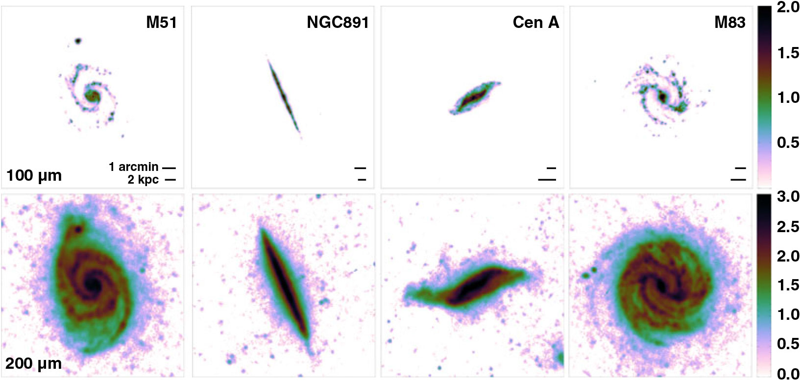
Figure 10. Expected signal-to-noise in 100  $\mu$m (top row) and 200 $\mu$m (bottom row) polarised intensity after 2 h on-source integration with B-BOP for four nearby ( $d\lt10$ Mpc) galaxies. The maps are constructed using Herschel data at 70 and 250 $\mu$m as input. We assume the B-BOP performance parameters given in Table 1, a dust spectral index of $\beta=1.9$, and a conservative polarisation fraction of 1%. The colour scale, which runs between a signal-to-noise ratio of 1 and 100 (top row) or 1 and 1 000 (bottom row), uses a logarithmic stretch, with green indicating a signal-to-noise of 10.
6.2.1. Testing and refining Galactic dynamo models
The currently favoured paradigm for interstellar magnetic fields is that they are amplified by dynamo action. In this scenario, weak primordial fields in young galaxies are quickly amplified by a small-scale turbulent dynamo, which continuously supplies turbulent fields to the ISM after the formation of a galactic disk in  $\mathbin{\lower.3ex\hbox{$\buildrel<\over {\smash{\scriptstyle\sim}\vphantom{_x}}$}} {10^9}$ yr (Schleicher et al. Reference Schleicher, Banerjee, Sur, Arshakian, Klessen, Beck and Spaans2010). The large-scale field is then amplified by the mean-field $\alpha - \Omega$ dynamo effect (e.g., Ruzmaikin, Sokoloff, & Shukurov Reference Ruzmaikin, Sokoloff and Shukurov1988), whereby the combination of differential rotation of the galactic disk ( $\Omega$-effect) and helical turbulence ( $\alpha$-effect), presumably driven by supernova explosions (Ferrière & Schmitt Reference Ferrière and Schmitt2000), produces small-scale magnetic loops and organises some fraction of them into regular large-scale patterns.
The mean field dynamo is expected to generate a regular magnetic field with both poloidal and azimuthal components, and nearly all polarised synchrotron observations of face-on disk galaxies show a large-scale spiral pattern. To date, the magnetic-field pitch angles  $p_{B}$ and azimuthal structure that have been observed in nearby disk galaxies via observations of polarised radio synchrotron emission are broadly compatible with the predictions of mean field dynamo theory (Fletcher Reference Fletcher, Kothes, Landecker and Willis2010; Van Eck et al. Reference Van Eck, Brown, Shukurov and Fletcher2015). Yet, the precise nature of the magnetic field generated via the mean-field dynamo depends on properties of the host galaxy. For example, the rotation curve determines the shear strength in a differentially rotating galaxy disk, and hence how the azimuthal field component is generated from the poloidal field. The $\alpha$-effect—by which a poloidal field component is generated from the azimuthal field—is thought to be powered by supernova explosions, which depend on a galaxy’s star formation rate. As our knowledge of external galaxies grows, the logical next step is to refine dynamo models for specific galaxies to include all relevant observed galaxy properties—e.g., the ionised and molecular gas density distributions, rotation curve, star formation rate, gas inflow and outflow rates—and test the model predictions for individual galaxies against the observed properties of the magnetic field. The first attempt to do this systematically for a sample of galaxies (Van Eck et al. Reference Van Eck, Brown, Shukurov and Fletcher2015) was hampered by inconsistencies in the available radio observations. A sample of galaxies observed with the same instrument at the same resolution and sensitivity is necessary to allow the details of dynamo theory, such as how the dynamo saturates, to be tested against data. B-BOP’s moderate resolution, full-disk sampling of the magnetic-field structure across a statistically significant sample of nearby galaxies would provide precisely this test.
6.2.2. Magnetic fields and gas flows in barred and spiral galaxies
Mapping the structure of the magnetic field across a sample of nearby galaxies is needed to understand the typical dynamical importance of the field on galactic scales. Of particular interest is how gas flows in galaxies—e.g., gas streaming along spiral arms, inflow along bar dust lanes, and starburst-driven outflows—interact with the field. While independent estimates of the field strength will still be required, B-BOP observations at sub-kiloparsec resolution of the magnetic-field structure and complementary spectral line data for tracing interstellar gas kinematics will be extremely valuable for studying the interplay between the field and motions within the cold gas reservoir across the local galaxy population.
In face-on disk galaxies, the large-scale field traced by radio polarisation observations tends to follow a spiral pattern. This pattern is expected from mean field dynamo theory, and is not directly connected to a galaxy’s baryonic (i.e., gas/stellar) spiral structure. Observations of spiral galaxies indeed show that the field pattern is not always spatially coincident with the spiral arms, and in several cases (most famously NGC6496 Beck Reference Beck2007) the ordered field pattern is most pronounced in the interarm region. Some of the large-scale field patterns in galaxies may be due to the combined action of shear and compression in the interstellar gas, which renders the turbulent field anisotropic (and hence ordered) over large scales (e.g., in M51, Fletcher et al. Reference Fletcher, Beck, Shukurov, Berkhuijsen and Horellou2011; Mulcahy et al. Reference Mulcahy2014, Reference Mulcahy, Fletcher, Beck, Mitra and Scaife2016). Current observations also suggest that the average pitch angle of the regular spiral field pattern is often similar to the pitch angle of the local spiral arm  $p_{M}$. This is not a direct prediction of mean-field dynamo theory, but would be expected if spiral shocks amplify the magnetic-field component parallel to the shock. Significant discrepancies between $p_{B}$ and $p_{M}$ in the inter-arm region, as well as large azimuthal and radial variations in $p_{B}$, are also observed, the origin of which are not yet well understood.
The central regions of barred galaxies are the site of fast radial gas inflow, strong shocks, and intense star formation. Barred galaxies often show strong gas streaming along the shock fronts at the edge of bars, which develop because the gas is rotating faster than the bar pattern. Radio polarisation observations of the prototypical barred galaxy NGC1097 (Beck et al. Reference Beck, Fletcher, Shukurov, Snodin, Sokoloff, Ehle, Moss and Shoutenkov2005) reveal strongly polarised emission along the bar with field orientations parallel to the gas streamlines. The observed polarisation pattern suggests that the field is amplified and stretched by shear in the compression region, and that the field is frozen into the gas and aligned with the gas flow over a large part of the bar. If this result holds generally in barred galaxies, the polarisation pattern in bars—especially using a tracer that preferentially probes the dense interstellar gas—would provide important complementary information on the plane-of-sky gas flows to the line-of-sight kinematic information obtained from molecular emission lines. In combination with estimates for the magnetic-field strength, information about the magnetic-field structure in the central regions of barred galaxies would also provide useful constraints for models of active galactic nuclei (AGNs) fuelling. One of the main problems in this area is to generate mass inflow rates that are compatible with the observed nuclear activity. Magnetic stress in circumnuclear rings (e.g., Beck et al. Reference Beck, Ehle, Shoutenkov, Shukurov and Sokoloff1999) and fast MHD density waves (e.g., Lou et al. Reference Lou, Yuan, Fan and Leon2001) have been proposed as potential mechanisms, but current observational data for the field strength and structure in the inner regions of barred galaxies are not sufficient for a rigorous test of these models.
6.2.3. Magnetism in dwarf galaxies
Due to their slow rotation, the amplification of magnetic fields should be less efficient in dwarf galaxies. Yet observations of radio polarised intensity show that several nearby low-mass galaxies host large-scale ordered fields, e.g., the Magellanic Clouds, NGC4449 and IC10 (Chyży et al. Reference Chyży, Knapik, Bomans, Klein, Beck, Soida and Urbanik2003; Gaensler et al. Reference Gaensler, Haverkorn, Staveley-Smith, Dickey, McClure-Griffiths, Dickel and Wolleben2005; Mao et al. Reference Mao2012; Chyży et al. Reference Chyży, Drzazga, Beck, Urbanik, Heesen and Bomans2016; Heesen et al. Reference Heesen2018). Dwarf galaxies are also more likely to exhibit star formation powered outflows and galactic winds, due to their shallow gravitational potential. The magnetised nature of these outflows has been observed in some dwarf systems (Chyży et al. Reference Chyży, Beck, Kohle, Klein and Urbanik2000; Kepley et al. Reference Kepley, Mühle, Everett, Zweibel, Wilcots and Klein2010), consistent with some models of a cosmic ray driven dynamo (Siejkowski et al. Reference Siejkowski, Otmianowska-Mazur, Soida, Bomans and Hanasz2014; Dubois & Teyssier Reference Dubois and Teyssier2010). To date, all dwarf galaxies with detected ordered magnetic fields are star-bursting, participating in a galaxy-galaxy interaction, and/or experiencing significant gas infall, suggesting the importance of enhanced turbulence for the magnetic-field properties and evolution of these systems. B-BOP observations of a sample of local dwarf galaxies with a range of masses, interaction properties and star formation histories, would provide valuable input for theories for the amplification of magnetic fields in such systems, and their role in magnetising the IGM.
6.2.4. The Magellanic Clouds
The Large and the Small Magellanic Clouds (LMC, SMC) are the closest gas-rich galaxies to the Milky Way. A B-BOP survey of the Magellanic Clouds would for the first time probe the magnetic-field structure in the cold ISM across all spatial scales between the clumpy sub-structure within GMCs ( ${\sim}2$ pc) and the galactic disk (several kpc). Observations across such a large range of spatial scales are needed to decipher the dynamical importance of the magnetic field for the inherently hierarchical process of star formation, i.e., from the formation of GMCs out of the diffuse ISM, down to the formation of individual stars. Spatially complete surveys of dust emission in the Magellanic Clouds with ALMA are unfeasible due to their large angular size ( ${\sim}50$ and ${\sim}10$ deg $^2$ for the LMC and SMC, respectively).
As an example of what could be achieved with B-BOP, Figure 11 shows the estimated signal-to-noise ratio for a 50-h polarimetric imaging survey of the LMC at 100, 200, and  $350\, \mu$m. This hypothetical survey would achieve a signal-to-noise ratio of 3 for the polarised intensity at 100 $\,\mu$m for interstellar gas with H column densities above ${\sim}2.5 \times 10^{21}$ cm $^{-2}$ (equivalent to $A_{V}\sim0.4$ in the LMC—Weingartner & Draine Reference Weingartner and Draine2001). This sensitivity would yield $\sim$0.5 million independent measurements of the magnetic-field orientation in the interstellar gas on spatial scales of 2 pc, including in the column-density regime of the atomic-to-molecular phase transition. At 200 and 350 $\mu$m, a similar number of significant detections of the magnetic-field orientation would be achieved in even more diffuse gas ( ${\sim}1 \times 10^{21}$ cm $^{-2} \approx 0.15$ mag). This represents $\sim$2 orders of magnitude increase in detail over measurements with Planck’s 353 GHz channel in the Magellanic Clouds, and would provide the first spatially complete view of the parsec-scale magnetic-field structure in the molecular gas reservoir of any galaxy.
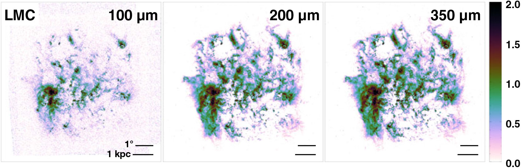
Figure 11. Expected signal-to-noise in polarised intensity for B-BOP observations of the LMC after 50 h on-source integration. The maps are constructed using Herschel data at 100 and 250  $\mu$m as input (Meixner et al. Reference Meixner2013). We assume the B-BOP performance parameters given in Table 1, a dust spectral index of $\beta=1.9$, and a conservative polarisation fraction of 1%. The colour scale, which runs between a signal-to-noise ratio of 1 and 100, uses a logarithmic stretch, with green indicating a signal-to-noise of 10.
6.2.5. Wavelength dependence of polarisation in U/LIRGs and AGNs
The polarisation of luminous external galaxies such as Luminous Infrared Galaxies (LIRGs), Ultraluminous Infrared Galaxies (ULIRGs), and AGNs, in the far-IR and submillimeter can arise from synchrotron emission but also from emission or absorption by aligned dust grains in the optically thick clouds that surround young stars and AGN tori (e.g., Efstathiou, McCall, & Hough Reference Efstathiou, McCall and Hough1997; Aitken et al. Reference Aitken, Efstathiou, McCall and Hough2002). Information in the far-IR and submillimeter can be combined with information at 10 and 18  $\mu$m as well as near-IR data from the ground to study the switch in position angle by about $90^\circ$ that is predicted as polarisation changes from dichroic absorption at shorter wavelengths to dichroic emission at longer ones. Several highly polarised galaxies in the mid-IR were found by Siebenmorgen and Efstathiou (Reference Siebenmorgen and Efstathiou2001) with the Infrared Space Observatory (ISO) and more recently by Lopez-Rodriguez et al. (Reference Lopez-Rodriguez2018a) with CanariCam on the 10.4-m Gran Telescopio Canarias (GTC).
This is a science area where significant progress can be achieved with B-BOP, which will provide sensitive polarisation measurements at 100–350  $\mu$m for a large sample of luminous external galaxies. Such information is currently available for very few objects. In a recent study of the nearby radio galaxy Cygnus A using data from HAWC+ onboard SOFIA, Lopez-Rodriguez et al. (Reference Lopez-Rodriguez, Antonucci, Chary and Kishimoto2018b) showed that this approach can be very useful for unravelling the polarisation mechanisms in the infrared and submillimeter and providing an independent method of estimating the contributions of AGN tori and starbursts to the SEDs. Exploring the role of AGNs and star formation in galaxies is a scientific objective of wide interest. The opportunity to study multi-wavelength polarisation with B-BOP will be complementary to other methods such as spectroscopy (e.g., González-Alfonso et al. Reference González-Alfonso2017) and traditional SED fitting of the total emission (e.g., Gruppioni et al. Reference Gruppioni2017).
6.3. Distant galaxies and the potential detection of the Cosmic Infrared Background polarisation
The build-up of coherent magnetic fields in galaxies and their persistence along cosmic evolution is being investigated with analytical models of the galactic dynamo (e.g., Rodrigues et al. Reference Rodrigues, Chamandy, Shukurov, Baugh and Taylor2019) and numerical simulations of galaxy formation (e.g., Martin-Alvarez et al. Reference Martin-Alvarez, Devriendt, Slyz and Teyssier2018). These studies suggest that the mean-field dynamo is effective early in the evolution of galaxies but, today, polarisation data available to trace the redshift evolution of galactic magnetic fields are very scarce (Mao et al. Reference Mao2017). While SKA holds exciting promises to extend observations of cosmic magnetism to the distant universe (e.g., Basu et al. Reference Basu, Mao, Fletcher, Kanekar, Shukurov, Schnitzeler, Vacca and Junklewitz2018; Mao Reference Mao2018), we argue here that B-BOP can also uniquely contribute providing the first polarimetric extragalactic survey at far-IR wavelengths.
To quantify what could be achieved with B-BOP, we consider the point source sensitivity of a polarimetric extragalactic survey for an integration time of 10 h per deg $^2$ (Table 1). At the detection limit of Herschel imaging surveys in total intensity, the signal-to-noise ratio of B-BOP in Stokes Q and U is ${\sim} 200$ at $200\, \mu$m and ${\sim} 100$ at 100 and $350\, \mu$m. This sensitivity needs to be compared to the few existing values of the far-IR polarisation fraction for galaxies as a whole.
The net polarisation fraction resulting from the integrated emission of galaxies depends on the existence of a coherent mean magnetic field and on viewing angle. In disk galaxies, the polarisation angle is aligned with the projection of the galaxy angular momentum vector on the plane of the sky, and the polarisation fraction increases from a face-on to an edge-on view. Integrating the Planck dust polarisation maps at 353 GHz over a  $20^\circ$ wide band centered on the Galactic plane, De Zotti et al. (Reference De Zotti2018) found a polarisation fraction $p= 2.7$%. Within a simple model, p is expected to scale as sin $\,i$, where i is the inclination angle of the galaxy axis to the line of sight. For this scaling, the mean p fraction averaged over inclinations is $1.4$. This may be taken as a reference value for spiral galaxies like the Milky Way, but p is likely to be on average lower for distant infrared galaxies. Indeed, SOFIA polarisation imaging of the two template starburst galaxies, M82 and NGC253, revealed regions with different polarisation orientations, which tend to average out when computing the integrated polarised emission yielding an overall mean $p \sim 0.1$% (Jones et al. Reference Jones2019).
Even if B-BOP only detects polarised emission from only a small fraction of Herschel galaxies, the number of detections will be significant given the present dearth of such measurements. If the detections are numerous, the emission from galaxies could even limit the polarisation sensitivity of B-BOP deep surveys. This is a possibility that needs to be assessed. Beyond the study of individual galaxies, we anticipate that the main outcome of a deep polarimetric extragalactic survey with B-BOP could follow from a statistical analysis of the data.
Statistical analysis is the reference in cosmology and much can be learned without detecting sources individually. In particular, the cross-correlation of surveys across the electromagnetic spectrum is a powerful means commonly used. In the far-IR, this is illustrated by the results obtained stacking Herschel data on positions of extragalactic sources in the near- and mid-IR. This approach has been successfully used to statistically identify sources accounting for the bulk of the Cosmic Infrared Background (CIB), although they were too faint to be detected individually (Béthermin et al. Reference Béthermin2012; Viero et al. Reference Viero2013). B-BOP, which will extend these studies to polarisation, is uniquely suited to detect—or set tight constraints on—the CIB polarisation. We note that the analysis of point sources circumvents the difficulty of separating the CIB from the foreground polarised emission of the diffuse Galactic ISM.
For polarisation, data stacking needs to be oriented to align polarisation vectors. This can be achieved by using, e.g., galaxy shapes measured from near-IR surveys at the appropriate angular resolution. Another interesting path will be the study of correlations between B-BOP extragalactic survey data and maps of the cosmic web inferred from weak-lensing surveys. The angular momenta of galaxies are not randomly oriented on the sky. The cosmic web environment has a strong influence on galaxy formation and evolution, and tidal gravitational fields tend to locally align the spins of dark-matter halos and galaxies. Such alignments, observed in dark-matter simulations, bear information on galaxy formation and evolution, as well as on the growth of structure in the Universe (Kirk et al. Reference Kirk2015). In this picture, low-mass haloes tend to acquire a spin parallel to cosmic web filaments, while the most massive haloes, which are typically the products of later mergers, have a spin perpendicular to filaments (e.g., Codis et al. Reference Codis, Pichon, Devriendt, Slyz, Pogosyan, Dubois and Sousbie2012; Dubois et al. Reference Dubois2014). Quasar observations provide observational evidence of a correlation between the polarisation orientation of galaxies and the large-scale structure of the Universe (Hutsemékers et al. Reference Hutsemékers, Braibant, Pelgrims and Sluse2014), but only for a small number of sources. B-BOP can uniquely contribute to characterising this correlation for infrared-luminous galaxies.
The scientific goals outlined here are new and promising but still qualitative. Modelling is required to assess the scientific outcome of a deep polarimetric extragalactic survey with B-BOP and decide on the best observing strategy in terms of survey depth and sky coverage.
7. Constraining dust physics
The polarisation of thermal dust emission depends on the shape, size, composition, and alignment efficiency of dust grains, and also on the 3D structure of the Galactic magnetic field on the line of sight and within the instrument beam. Dust polarised emission can therefore bring specific constraints on the alignment mechanism of dust grains and possibly on the grain shape. Despite this complex nature, it can also be used to constrain the optical properties of aligned dust grains (emissivity, spectral index), which are large grains at thermal equilibrium (Planck int. res. XXI 2015; Planck int. res. XXII 2015).
As described below, B-BOP, with its high angular resolution and good wavelength coverage of the polarised dust SED, will be a key instrument to provide new constraints on grain alignment theories and inform the evolution of aligned grain properties from the diffuse ISM to the densest cloud cores.
7.1. Probing the grain alignment mechanism
Grain alignment is subordinate to various processes. First, grains must rotate supra-thermallyFootnote l to be well aligned. Radiative torques, or chemical torques resulting from the formation of H $_2$ molecules on the surface of grains, are good candidates for grain spin-up. Second, alignment torques of magnetic, radiative, or mechanical origin (Hoang & Lazarian Reference Hoang and Lazarian2016) are needed to align the supra-thermally rotating dust grains. Compared to the time evolution of MCs and cores, the alignment of grains along magnetic-field lines by radiative torques is a fast process, with a timescale on the order of $10^3$– $10^4\,$ yr (Hoang & Lazarian Reference Hoang and Lazarian2014),Footnote m so that situations where grain alignment would be out-of-equilibrium can be safely ignored.
While the mechanisms of dust grain alignment are still debated (see, e.g., Section 2.1.1), polarisation measurements at UV to optical wavelengths imply that the alignment efficiency of dust grains is sensitive to grain size. Such a behaviour, well observed in the Mie regime where absorption and scattering are size-dependent (Bohren & Huffman Reference Bohren and Huffman1983), is however more difficult to extract from the polarised thermal SED because the dust temperature and dust spectral index depend more on the grain shape, internal structure, and composition (through its emissivity) than on the exact grain size.
As already mentioned in Section 2.1.1, the leading grain alignment theory is RATs (e.g., Lazarian & Hoang Reference Lazarian and Hoang2007, and references therein). The RATs alignment mechanism, if present, will lead to characteristic signatures in observations. For instance, in this theory, the alignment efficiency is directly dependent on the angle between the incident radiation field and the magnetic-field direction ( $\psi$). When dust is heated by a single nearby star or in starless dense cores where the field is strongly attenuated and anisotropic, the incident radiation field direction is well characterised. Since the magnetic-field orientation projected on the plane of the sky can be determined from the polarised signal, mapping dust polarisation in such regions can in principle be used to test alignment by RATs. This is illustrated in Figure 12 which sketches the relative geometry of the radiation field and magnetic field in a region of the ISM where the radiation field is dominated by a single star. In such regions, the RATs alignment theory predicts a stronger alignment, and therefore, a higher polarisation fraction where $\psi$ is close to $0^\circ$.
Figure 12. Sketch of the geometry around a single star dominating the heating of the local ISM. The magnetic-field direction is represented by the horizontal dashed lines. The aligned dust grains are sketched as prolate rotating parallelograms. If RATs dominate, dust alignment will be more efficient in regions with low values of  $\psi$, the angle between the stellar radiation and magnetic-field directions. Source: Figure adapted from Potter (Reference Andersson and Potter2010) and Andersson et al. (Reference Andersson, Pintado, Potter, Straižys and Charcos-Llorens2011).
Despite an expected clear signature, direct observational evidence of this angular effect has been scarce. The only positive detection reported in emission is by Vaillancourt and Andersson (Reference Vaillancourt and Andersson2015) who detected a periodic modulation of the dust polarisation fraction around the Becklin–Neugebauer Kleinmann–Low (BN-KL) object in Orion OMC-1. Some authors also claim to have evidenced a correlation between dust temperature and polarisation fraction, as expected for dust grains aligned through the RATs mechanism (Andersson et al. Reference Andersson, Pintado, Potter, Straižys and Charcos-Llorens2011; Matsumura et al. Reference Matsumura, Kameura, Kawabata, Akitaya, Isogai and Seki2011). There are also a few reports that indicate a possible influence of H $_2$ formation (e.g., Andersson et al. Reference Andersson2013, in IC63). In any case, only a handful of cases have been investigated so far and there is certainly a bias in the literature for publishing detections rather than non-detections. Given the intrinsically tangled nature of magnetic-field geometry, chance coincidences are very difficult or even impossible to exclude for these few isolated studies and a statistically representative study is clearly needed.
Such a study has not been carried out so far using Planck all-sky data, essentially because the number of interstellar regions where dust is directly and predominantly heated by a single star is very low at the Planck angular resolution. Attempts to unambiguously detect a statistical increase of the polarisation fraction with dust temperature in the Planck data, which would also be attributable to radiation-enhanced spin-up and alignment of dust grains, have not led to a strong conclusion. Planck 2018 res. XII (2019) showed that it is possible to disentangle, statistically, between what can be attributed to variations in grain alignment efficiency or grain properties, and what is due to line of sight and beam averaging of magnetic-field structures. This study demonstrated that there is no strong variations in grain alignment efficiency in the diffuse ISM (up to a column density,  $N_{\rm H} \sim 2\times10^{22}$ cm $^{-2}$), but, due to the low angular resolution of the Planck data, could not conclude in the case of the high-density ISM. Planck 2018 res. XII (2019) did not find any correlation either between dust temperature and polarisation fraction in the diffuse ISM. In conclusion, the analysis of the Planck all-sky data have so far not allowed to strongly confirm or rule out any specific grain alignment theory, but have provided an upper limit to the drop of alignement in the diffuse ISM.
Owing to its much higher angular resolution and sensitivity, B-BOP will allow us to systematically map the polarisation of dust emission around thousands of individual stars heating the nearby ISM locally. The good coverage of the polarised SED will allow us to measure the temperature of aligned dust grains responsible for the polarised emission. Analysis of the polarisation fraction as a function of the angle between the known radiation field and the magnetic-field direction derived from polarisation will allow us to test, for the first time, the RATs alignment theory with statistical significance, in a way that is not affected by local variations and the complexity of individual objects. At the same time, we will be able to detect, if present, the polarised emission resulting from the small temperature difference between grains heated face-on and edge-on immersed in an anisotropic radiation field (Onaka Reference Onaka1995). This process, which is only efficient at short wavelength ( $\lambda \le 100\,\mu$m, Onaka Reference Onaka2000), would appear in B-BOP data as a characteristic difference between the polarisation fraction and angle measured at $100\,\mu$m and the ones measured by unaffected channels at longer wavelengths.
Altogether, the high resolution, sensitivity, and spectral coverage of B-BOP will set unprecedented, probably unexpected constraints on the physics of grain alignment in star-forming regions, a topic which Planck observations could hardly address.
7.2. Dust polarisation as a proxy for dust evolution
The wavelength range covered by B-BOP will allow us to disentangle between various dust models. The Wien part of the polarised dust emission is currently not constrained. It is in this wavelength range that dust models present the strongest differences in spectral variations of  $P/I$ (Figure 13), in particular, between those where carbon grains are aligned and those where they are not (Draine &Hensley Reference Draine and Hensley2013; Guillet et al. Reference Guillet2018). Moreover, as dust models now predict both emission and absorption properties of dust grain populations in polarisation (Siebenmorgen, Voshchinnikov, & Bagnulo Reference Siebenmorgen, Voshchinnikov and Bagnulo2014; Draine & Hensley Reference Draine and Hensley2017; Guillet et al. Reference Guillet2018), joint observations of common targets with B-BOP and survey experiments targeting extinction polarisation of background stars, such as PASIPHAE (Tassis et al. Reference Tassis2018), can be used to further test such models.
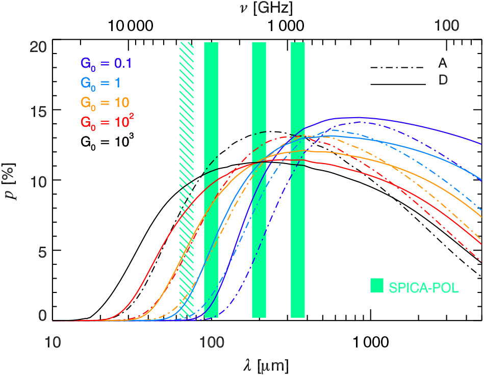
Figure 13. Polarisation fraction as a function of wavelength predicted using the DustEM (http://www.ias.u-psud.fr/DUSTEM) numerical tool (Compiègne et al. Reference Compiègne2011; Guillet et al. Reference Guillet2018). The vertical bands show the B-BOP photometric channels. The dashed band shows a suggested shifted location for the short-wavelength band of B-BOP at  $70\,\mu$m, which would better cover the Wien part of the polarised dust SED. In model A, only silicate grains are aligned, while carbon grains are randomly aligned. In model D, both silicate and carbon are aligned, with carbon inclusions incorporated in the silicate matrix (6% in volume). Source: Figure adapted from Guillet et al. (Reference Guillet2018).
High-resolution polarisation observations with B-BOP will allow us to probe dust properties in dense environments and to further characterise dust evolution between diffuse and dense media (e.g., Köhler, Ysard, & Jones Reference Köhler, Ysard and Jones2015). Observationally, a number of studies based on emission and extinction data have provided evidence of grain growth within dense clouds. One of the main results is an increase of the far-IR/submillimeter emissivity by a typical factor of 2–3 compared to standard grains in the diffuse medium (cf. Stepnik et al. Reference Stepnik2003; Planck early res. XXV 2011; Ysard et al. Reference Ysard2013; Roy et al. Reference Roy2013; Juvela et al. Reference Juvela2015), as predicted by calculations of aggregate optical properties (Ossenkopf & Henning Reference Ossenkopf and Henning1994; Köhler et al. Reference Köhler, Stepnik, Jones, Guillet, Abergel, Ristorcelli and Bernard2012, Reference Köhler, Ysard and Jones2015). Another striking result is the so-called coreshine effect, i.e., enhanced mid-IR light scattering detected with Spitzer towards a number of dense cores (Pagani et al. Reference Pagani, Steinacker, Bacmann, Stutz and Henning2010; Steinacker et al. Reference Pagani, Steinacker, Bacmann, Stutz and Henning2010), implying the presence of larger (Steinacker et al. Reference Steinacker2015) or, taking into account the change in dust optical properties, only moderately larger (Ysard et al. Reference Ysard, Köhler, Jones, Dartois, Godard and Gavilan2016) dust grains.
Stochastic emission by very small grains ( $a\ll 10$ nm) is known to contribute significantly to the 60 and 100 $\mu$m emission bands. This contribution is estimated to be on the order of 13% at 100 $\mu$m and 45% at 60 $\mu$m (e.g., Jones et al. Reference Jones, Fanciullo, Köhler, Verstraete, Guillet, Bocchio and Ysard2013). When the 100 $\mu$m band is used to derive the dust temperature, this contamination affects the accuracy of mass determinations using dust continuum measurementsFootnote n. The formation of dust aggregates first removes the very small grains from the gas phase, as suggested by observations showing a significant decrease in the 60 $\mu$m emission (Laureijs, Clark, & Prusti Reference Laureijs, Clark and Prusti1991; Bernard et al. Reference Bernard1999; Stepnik et al. Reference Stepnik2003; Ysard et al. Reference Ysard2013) and as predicted by dust evolution models (Ossenkopf & Henning Reference Ossenkopf and Henning1994; Köhler et al. Reference Köhler, Ysard and Jones2015). Because small grains are not aligned with the magnetic field, such contamination is absent from the polarised thermal emission SED.Footnote o As a consequence, the dust temperature derivedFootnote p from the polarised dust SED that B-BOP can observe will only reflect the temperature of large aligned dust grains in the transition from the diffuse to the dense ISM, a constraint that will be used in addition to that inferred from the total intensity SED to study dust evolution processes.
Just like unpolarised emission, polarised dust emission will also probe variations in dust emissivity as expected from dust evolution in dense clouds. Dense environments could not be properly characterised in polarisation at the low resolution of the Planck data. Unlike unpolarised emission, the anisotropic nature of polarised emission makes it sensitive to the grain shape. The formation of dust aggregates by grain–grain coagulation must have its counterpart in polarisation, and B-BOP will detect signatures which will have to be analysed through detailed modelling of the coagulation process. Here again, the combination of B-BOP data with the increasing amount of high-resolution polarisation observations in the optical and the near-IR will provide strong constraints on dust evolution (Planck int. res. XXI 2015; Planck 2018 res. XII 2019).
Observations of total dust emission intensity at far-IR and submillimeter wavelengths with Planck and Herschel have also brought surprises. One of them is evidence that the logarithmic slope of the dust emission SED at long wavelengths, often referred to as the dust emissivity index,  $\beta$, exhibits significant variations at large scales across the Galaxy. The Planck all-sky data clearly show variations of $\beta$ along the Galactic plane, from very steep SEDs towards inner regions of the Milky Way to much flatter SEDs ( $\beta \simeq1.5$) towards the Milky Way anticenter (Planck 2013 res. XI 2014). This has also been confirmed in the far-IR by the analysis of Hi-GAL data (Paradis et al. Reference Paradis2012). Even larger variations have been found in observations of external galaxies, with the SMC and LMC having $\beta\simeq1.3$ and $\beta\simeq1.0$, respectively (Planck early res. XVII 2011). Such variations are observed in the Herschel data within individual nearby galaxies such as M31 (Smith et al. Reference Smith2012) and M33 (Tabatabaei et al. Reference Tabatabaei2014). The origin of these variations is currently unclear and three main classes of dust models have been proposed to explain them. The first type involves the mixing of different materials during the dust life-cycle (Köhler et al. Reference Köhler, Ysard and Jones2015; Ysard et al. Reference Ysard, Köhler, Jones, Miville-Deschênes, Abergel and Fanciullo2015). The second type of models invokes Two-Level-System (TLS) low-energy transitions in the amorphous material composing dust grains (Meny et al. Reference Meny, Gromov, Boudet, Bernard, Paradis and Nayral2007) as the cause for the flattening of the SED. The third type of models proposes that magnetic inclusions in dust grains (Draine & Hensley Reference Draine and Hensley2013) could produce the observed variations (Draine & Hensley Reference Draine and Hensley2012). Determining the origin of these variations is critical in many respects, not only to understand the dust cycle in the ISM, but also for accurate mass determinations from dust continuum measurements (which require good knowledge of the dust emissivity, its wavelength dependence, and its spatial variations).
In this domain again, extensive polarimetric imaging at far-IR wavelengths is likely to play a critical role in the future. Dust models based on dust evolution have not yet presented their predictions in polarisation, but the other two classes of models mentioned above predict significantly different behaviours for the polarisation fraction as a function of wavelength. TLS-based models essentially predict a flat spectrum for the polarisation fraction, a prediction compatible with Planck observations. In contrast, metallic-inclusion models predict variations of the polarisation fraction in the submillimeter (Draine & Hensley Reference Draine and Hensley2013), which are not observed. It will be possible to evidence those distortions of the polarisation SED by comparing far-IR B-BOP observations with existing submillimeter Planck data for the Magellanic Clouds and polarisation data obtained with new ground-based polarimetric facilities such as NIKA2-POL and SCUBA2-POL for Milky Way regions/sources and nearby galaxies. Correlating changes in the polarised SED with variations of  $\beta$ will allow us to constrain models of the submillimeter dust emissivity in a very unique way.
7.3. Towards a tentative detection of polarisation by dust self-scattering in the densest cores
In the past decade, interesting constraints on grain sizes in dense clouds have come from the detection of the ‘coreshine’ effect (Pagani et al. Reference Pagani, Steinacker, Bacmann, Stutz and Henning2010), which results from scattering of near-IR stellar photons by dust grains present in the cloud. This has been interpreted as evidence of grain growth ( $a=1\, \mu$m, Steinacker et al. Reference Steinacker, Pagani, Bacmann and Guieu2010) or grain compositional and structural evolution with a modest size increase ( $a\lt0.5\, \mu$m, Ysard et al. Reference Ysard, Köhler, Jones, Dartois, Godard and Gavilan2016). More recently, it has been demonstrated that very large ( $a \gt 10\, \mu$m) dust grains are able to produce polarisation by scattering thermal dust emission, a process that is called ‘self-scattering’. This was first predicted to be observable in protoplanetary disks (Kataoka et al. Reference Kataoka2015) and then confirmed by numerous ALMA observations (Kataoka et al. Reference Kataoka, Muto, Momose, Tsukagoshi and Dullemond2016; Yang et al. Reference Yang, Li, Looney, Girart and Stephens2017; Girart et al. Reference Girart2018).
B-BOP, with its 100  $\mu$m polarised channel, would be able to detect and characterise the spectral dependence of polarisation by scattering due to ${\sim} 15$ $\mu$m dust grains (Kataoka et al. Reference Kataoka2015), if present. For the effect to be observable, the thermal emission of dust must first present a quadrupolar anisotropy: scattering grains must receive more far-IR irradiation along one direction in the plane of the sky than along the perpendicular direction. Such a condition is naturally met in a dense protostellar core or in the presence of density gradients. Second, high local densities ( ${>}10^6\, {\rm cm}^{-3}$) must be present along the line of sight so that dust grains can have grown to the very large sizes ( $a \sim \lambda/2\pi$) needed for scattering to occur in the far-IR. Observing such a high-density medium should be feasible at $100\,\mu$m at the resolution of SPICA, but simulations of grain growth and polarisation by scattering are needed to confirm this idea.
Polarisation by self-scattering at  $100\,\mu$m with B-BOP will most likely concern only a few lines of sight through the densest cores. Because polarisation due to scattering sharply declines at wavelengths larger than the grain size, it will not alter the polarised emission from aligned dust grains at 200 and $350\,\mu$m used to trace the local magnetic-field orientation in MCs (Sections 2–5).
8. Molecular clouds and the origin of cosmic rays
Polarimetric imaging of MCsFootnote q with B-BOP will also be very useful for the study of the origin of cosmic rays (CRs). Indeed, CRs pervade the whole galaxy, and their interaction with the dense gas of MCs has two important consequences. First, the interactions of high energy CRs (kinetic energy larger than a few 100 MeV) with the gas make MCs bright  $\gamma$-ray sources. Second, CRs of low energy ( $\approx 1{-}100$ MeV) are the only ionising agents able to penetrate MCs and regulate the ionisation fraction of MC dense cores. For these reasons, observations of enhanced levels of $\gamma$-ray emission or ionisation rates from MCs reveal the presence of a CR accelerator in their vicinity (see review by Gabici & Montmerle Reference Gabici and Montmerle2015).
A first problem arises, that of the propagation of cosmic rays inside MCs, for which the strength, and above all, the topology of the magnetic field around and inside them plays a central role. At high energies, CRs are unaffected by the magnetic field, so that they interact with all the gases (atomic as well as molecular): the  $\gamma$-ray emissivity is simply proportional to the product (CR flux $\times$ cloud mass). In other words, for a given cloud mass, determining the $\gamma$-ray luminosity of a MC allows the local CR flux to be measured, irrespective of the magnetic field. Over galactic scales, it is well established that the CR flux deduced in this way is essentially uniform (Ackermann et al. Reference Ackermann2011), which means that the CR diffusion away from their sources is efficient enough not to be sensitive to large-scale spatial features like the spiral arms. However, there may be $\gamma$-ray ‘hot spots’ close to CR sources, and this is precisely what happens when a supernova remnant (SNR) collides or is located in the vicinity of a MC. Many examples of such SNR-MC associations are known (Gabici & Montmerle Reference Gabici and Montmerle2015). The reason for the enhanced $\gamma$-ray emission is that SNR shock waves accelerate CR in situ, via the so-called Diffuse Shock Acceleration, or DSA, mechanism (Drury Reference Drury1983), so this particular configuration can be considered as a ‘CR laboratory’: if the shock-accelerated CRs are insensitive to the local magnetic fields when they reach high energies, the process by which they do, in other words the acceleration mechanism itself depends very much on it, and again on its topology close to the SNR shock. For instance, it is well known from theoretical DSA models that the acceleration efficiency depends strongly on the angle between the shock front and the local magnetic-field lines (Caprioli & Spitkovsky Reference Caprioli and Spitkovsky2014). So, again, knowing the magnetic-field topology on small spatial scales in MCs impacted by SNRs would allow a detailed study of the CR acceleration process in the vicinity of the shock front.
In particular, a new picture of the ISM in star-forming regions has now to be taken into account: in the standard picture summarised above, the gaseous medium in which the SNR shock propagates is assumed uniform. But as recent work has shown (see Section 2.2 and Figure 1), the structure of MCs is not uniform, but filamentary, down to scales of parsecs (in length) and  ${\sim} 0.1$ pc (in width), i.e., precisely those that are accessible to B-BOP at distances ${\approx} 1$ kpc. One of the key changes is then that the shock would cross the ambient magnetic-field lines at all angles, and likely perturb them and enhance the turbulent component of the magnetic field, on spatial scales comparable to that of the filaments: for not-too-distant sources, B-BOP would then act as a ‘magnifying-glass’ to study the shock-ambient gas interactions at unprecedented small spatial scales, and put entirely new, perhaps even unexpected, constraints on DSA models (e.g., see the CR escape issues raised by Malkov et al. Reference Malkov, Diamond, Sagdeev, Aharonian and Moskalenko2013).
At low energies, the situation is markedly different, because the transport properties of CRs become very sensitive to a variety of processes governed by the magnetic-field properties which may hamper the penetration of CRs into MCs, and reduce the rate at which the gas is ionised by these particles (Phan, Morlino, & Gabici Reference Phan, Morlino and Gabici2018). Like  $\gamma$-ray production at high CR energies, the ionisation by low-energy CR can also be measured by way of infrared and millimeter-wave observations, which detect lines of various molecules and radicals (like H $^+_3$, HCO $^+$, DCO $^+$, etc.—cf. Indriolo et al. Reference Indriolo2015). This has been done for many MCs in the Galaxy, but more recently also for SNR-MC collision regions (Gabici & Montmerle Reference Gabici and Montmerle2015): here again an enhancement of MC ionisation has been observed. The results tentatively suggest a proportionality between the SNR-accelerated high-energy and low-energy CR fluxes, constraining the acceleration mechanism, or a proportionality between the partially irradiated, ionised gas, and the fully irradiated, $\gamma$-ray emitting gas, or both.
More generally, both low- and high-energy CRs are affected in their propagation in the diffuse ISM by diffusion effects, which are still poorly known—and directly influenced by magnetic fields. The spatially average diffusion coefficient of CRs in the Galaxy is constrained by a number of observations, and is often assumed to be isotropic on large Galactic scales ( ${\gg} 100$ pc). On the other hand, in order to explain a number of $\gamma$-ray observations of SNR-MC associations (characterised by spatial scales of ${\sim} 10{-}100$ pc), a diffusion coefficient about 2 orders of magnitudes smaller (i.e., slower bulk propagation) than the average Galactic one needs to be assumed. However, such a discrepancy could be reconciled if CR diffusion is in fact anisotropic on such small scales (Nava & Gabici Reference Nava and Gabici2013). An anisotropic diffusion is indeed expected for spatial scales smaller than the magnetic-field coherence length (Malkov et al. Reference Malkov, Diamond, Sagdeev, Aharonian and Moskalenko2013). Knowing the topology of the magnetic field in such regions is thus of paramount importance in order to interpret $\gamma$-ray observations correctly.
All of these issues can be illustrated by a recent study of the W28 SNR (cf. Figure 14), a well-known example of an SNR-MC collision (Vaupré et al. Reference Vaupré, Hily-Blant, Ceccarelli, Dubus, Gabici and Montmerle2014). This SNR is located in the Galactic plane, at  $d \approx 2$ kpc from the Sun, with an estimated (very uncertain) age $\approx 10^4$ yr. At this distance, the SNR apparent diameter ( ${\sim} 30'$) gives a linear diameter $D \approx 20$ pc. An observation by the High Energy Stereoscopic System (HESS) Čerenkov telescope, in the TeV $\gamma$-ray range (Aharonian et al. Reference Aharonian2008), covering a large field-of-view of ${\sim} 1.5^\circ \times 1.5^\circ$ (with a resolution of ${\sim} 0.1^\circ$), has revealed a complex of several resolved $\gamma$-ray sources. One of the sources, which is spatially correlated with a part of the SNR shock outline, was also detected as a bright GeV source by the Fermi satellite, contrary to the other sources, which are either dimmer or undetected (Abdo et al. Reference Abdo2010). This multiple source was soon correlated with a complex of MCs mapped in CO by the NANTEN Footnote r telescope, showing that the SNR was in fact colliding with the MC associated with the GeV–TeV source (a physical contact being confirmed by the existence of several OH masers), the other sources being away, far upstream of the SNR shock.
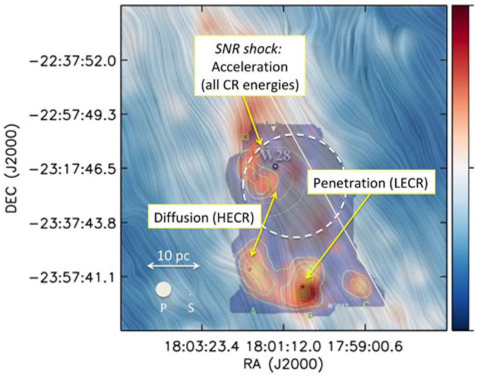
Figure 14. The region surrounding the W28 SNR ( $d \sim 2$ kpc; shock approximated by the dashed white circle), as seen in cold dust emission at $353\, $GHz by Planck (colour image with background B-field ‘drapery’ from polarisation data), in TeV–GeV $\gamma$-rays (white contours), and CO (green areas, well correlated with the $\gamma$-ray sources—Aharonian et al. 2008). The labels highlight the various CR processes discussed in the text, at high energies (HECR) and low energies (LECR). The Planck and B-BOP beams are indicated by a small circle (label ‘P’) and a dot (label ‘S’), respectively.
Calculations indicated a factor  $\approx 100$ enhancement of the local high-energy CR flux, qualitatively consistent with a local CR acceleration by the SNR shock. Using the IRAM 30-m telescope to observe various molecular and radical tracers (H $^{13}$CO $^+$, C $^{18}$O, etc.) in the millimeter range, Vaupré et al. (Reference Vaupré, Hily-Blant, Ceccarelli, Dubus, Gabici and Montmerle2014) were also able to calculate the MC ionisation rate $\zeta$ at several locations. They found ${\sim}$2–3 order of magnitude enhancements of $\zeta$ (or lower limits) over its average Galactic value ( $\zeta_0 \approx 4-5 \times 10^{-17} \rm{erg~s}^{-1}$—e.g., Indriolo et al. Reference Indriolo2015), for the cloud correlated with GeV–TeV emission, i.e., indirect evidence for a similar enhancement of the low-energy CR flux, but no such enhancements for the clouds far upstream of the SNR shock. Within the ‘GeV–TeV bright’ cloud, the measurements were separated by the IRAM telescope resolution, ${\sim} 12\, \text{arcsec}$, i.e., comparable to (only 1.5 times better than) the B-BOP resolution at $200\, \mu$m (or a linear scale ${\sim} 0.15$ pc). The (projected) distance to the other clouds is ${\sim} 10$ pc, and this is seen as the diffusion length for high-energy CRs (TeV CRs reaching the distant clouds before the GeV CRs).
Thus, the W28 SNR and its environment provide us with a case study with all the ingredients needed to improve our understanding of the origin of CRs, and their relation with magnetic fields down to scales  ${\sim} 0.15$ pc, i.e., much smaller than observable before: (i) CR acceleration by the SNR shock; (ii) diffusion of CRs between clouds as a function of energy; (iii) penetration of low-energy CRs in ‘average’ clouds, irradiated only by ambient, galactic CRs (cf. Figure 14).
For more distant sources, the ‘magnifying-glass’ effect of B-BOP on small spatial scales would of course decrease, but an interesting link could then be established with the Čerenkov Telescope Array (CTA, presently under construction; Actis et al. Reference Actis2011), which operates in the 20 GeV–300 TeV regime. Until CTA actually observes, it is difficult to make accurate predictions on how far SNR-MC systems such as W28 could be detected in  $\gamma$-rays. For CR studies, the main point is not simply the detection, but the location of the emission with respect to the shock. For the moment, only two cases are known in which the $\gamma$-rays are clearly upstream of the shock: W28 (detected by CGRO, Fermi and HESS, so from GeV to TeV energies), and W44 (detected by Fermi only, so at GeV energies only). About 20% of HESS sources, and most of the SNRs detected by Fermi are SNR-MC systems (H.E.S.S. Collab. et al. Reference Collab2018; Ackermann et al. Reference Ackermann2011), but apart from W28 and W44 it is difficult to distinguish between upstream and downstream $\gamma$-ray emissions (or both). Taking into account that CTA is $\sim$10 times more sensitive than HESS, and taking W28 as a template, representative of a Galactic disk SNR-MC population, we estimate that $\approx$10 W28-like sources could be possibly detected and be sufficiently resolved by CTA, hence be good targets for future B-BOP observations, which would in turn spur new theoretical work on CR acceleration on very small spatial scales not considered at present.
9. Polarised dust emission from protoplanetary disks
As already mentioned in Section 2, magnetic fields may regulate the gravitational collapse and fragmentation of prestellar dense cores, thereby influencing the overall star formation efficiency (Mouschovias & Ciolek Reference Mouschovias, Ciolek, Lada and Kylafis1999; Dullemond et al. Reference Dullemond, Hollenbach, Kamp, D’Alessio and Reipurth2007; Crutcher Reference Crutcher2012). It is thus natural to expect that, during core collapse, magnetic fields can be dragged inward, leaving a remnant field in the protoplanetary disk formed subsequently.
If protoplanetary disks are indeed (weakly) magnetised, then the MHD turbulence arising from magneto-rotational instability (MRI) is thought to be the primary source of disk viscosity, a crucial driving force for disk evolution (e.g., disk accretion) and planet formation (Balbus & Hawley Reference Balbus and Hawley1998; Turner et al. Reference Turner, Fromang, Gammie, Klahr, Lesur, Wardle, Bai and Beuther2014). Despite this general consensus, our knowledge about magnetic fields in disks is actually very limited and incomplete at this stage, largely due to the lack of observational constraints on magnetic-field properties (geometry and strength) in protoplanetary disks. Polarimetric observations of thermal dust emission at centimeter or millimeter wavelengths with single-dish telescopes, such as the Caltech Submillimeter Observatory (CSO) and JCMT, or interferometric arrays, such as the Karl G. Jansky Very Large Array (JVLA), the SMA, the Berkeley–Illinois–Maryland Array (BIMA), and the Combined Array for Research in Millimeter-wave Astronomy (CARMA), have been used extensively to map magnetic-field structure in YSOs at scales from  ${\sim} 50\,$AU to thousands of AU (see Crutcher Reference Crutcher2012 for a review). However, due to the limited sensitivity and angular resolution offered by current facilities and the nature of centimeter/millimeter observations, most of these studies have been focused on magnetic fields in molecular clumps/cores (cf. Section 4), or Class 0/Class I objects (e.g., Qiu et al. Reference Qiu, Zhang, Menten, Liu and Tang2013; Rao et al. Reference Rao, Girart, Lai and Marrone2014; Liu et al. Reference Liu2016), rather than classical protoplanetary disks around Class II objects. Using CARMA, Stephens et al. (Reference Stephens2014) spatially resolved the HL Tau disk in polarised light at 1.3 mm, and their best-fit model suggested that the observation was consistent with a highly tilted (by $\sim$50 $^\circ$ from the disk plane), toroidal magnetic field threading the disk. This conclusion was challenged by follow-up studies, which showed that the 1.3 mm polarisation of HL Tau could also arise solely from dust scattering as opposed to dichroic emission from elongated grains aligned with the magnetic field (Kataoka et al. Reference Kataoka2015; Yang et at. Reference Yang, Li, Looney, Cox, Tobin, Stephens, Segura-Cox and Harris2016). However, more recent ALMA observations at 0.87, 1.3, and 3.1 mm indicated that dust scattering alone may not be able to explain all of the multi-wavelength polarisation data (Kataoka et al. Reference Kataoka, Tsukagoshi, Pohl, Muto, Nagai, Stephens, Tomisaka and Momose2017; Stephens et al. Reference Stephens2017).
Recently, Li et al. (Reference Li, Pantin, Telesco, Zhang, Wright, Barnes, Packham and Mariñas2016) have been able to highlight the signature of a magnetic field in the AB Aur protoplanetary disk at mid-IR wavelengths. Using observations of the AB Aur protoplanetary disk at 10.5  $\mu$m with the GTC/CanariCam imager and polarimeter, they detected a polarisation pattern in the inner regions of the disk compatible with dichroic emission polarisation produced by elongated grains aligned by a tilted poloidal magnetic field. The observed polarisation level (2–3%) was somewhat lower than that predicted by theory (Cho & Lazarian Reference Cho and Lazarian2007), although this is something naturally expected since the modelling assumes alignment efficiencies and intrinsic particles polarisability which are probably overestimated. At a wavelength of 10.5 $\mu$m where protoplanetary disks are optically thick, the observations are probing the disk properties down to depths corresponding to the $\tau$ = 1 optical depth surface. This depth is relatively small (less than $\sim$10%) compared to the disk scale height. Longer wavelengths, up to about 200 $\mu$m where the disk can still be moderately optically thick up to large distances from the star, are emitted by cooler material located deeper within the disk. Thus, by measuring the level of polarisation at wavelengths in the range 100–300 $\mu$m, we expect to be able to compare the levels of polarisation as a function of optical thickness, thereby getting an indirect signature of the magnetic field at different depths within protoplanetary disks. This will provide constraints on the importance of MRI-induced turbulence. Together with 10 $\mu$m and ALMA similar types of observations, this will allow us to build a tomographic view of the magnetic field along the vertical profile of the disks. Such measurements would also have large impacts on our understanding of planet formation processes.
For the purpose of this paper, we used the same modelling approach as described in Li et al. (Reference Liu2016), with also the same disk parameters based on the example of AB Aur, in order to predict expected polarisation levels levels at 100, 200, and 350  $\mu$m if observed by SPICA. Given the angular resolution of SPICA at these wavelengths, we do not expect, apart from exceptional cases, to angularly resolve the polarised emission, therefore, we computed an integrated value, considering the object as unresolved.
In Figure 15, we show the predictions of the model, integrated over the full spatial extent of the disk, for different disk inclinations with respect to the line of sight and for observing wavelengths within the B-BOP range. Two types of magnetic-field configuration are considered, poloidal and toroidal, which are the simplest ones, and those also widely discussed in the literature. We can see from the simulations that the poloidal magnetic-field configuration produces stronger integrated polarisation signatures compared to the toroidal configuration.
Figure 15. Spatially integrated polarisation levels expected at 100–400 $\, \mu$m from magnetised protoplanetary disks as a function of disk inclination (0 $^\circ$ refers to a pole-on disk configuration). The left panel (a) considers a poloidal magnetic-field topology, and the right panel (b) a toroidal one. See Li et al. (Reference Liu2016) for more details about the assumptions of the disk model and the adopted parameter values.
As mentioned earlier, the origin of the dust continuum polarisation on the disk scale is still uncertain, with potential contributions from scattering by large grains in addition to that from emission by magnetically (or radiatively) aligned grains. The B-BOP instrument will generally not (or barely be able to) resolve protoplanetary disks, which poses the problem of disentangling these various mechanisms. Fortunately, polarisation by aligned dust grains and polarisation by dust self-scattering have different dependences on wavelength and optical depth (Yang et al. Reference Yang, Li, Looney, Girart and Stephens2017). SPICA will greatly extend the wavelength coverage of ALMA (from 870 to 100 $\, \mu$m), which will make it easier to disentangle the contributions from the competing mechanisms. Such an effort is a pre-requisite for using dust continuum polarisation to probe both disk magnetic fields and grain growth, the crucial first step towards the formation of planetesimals and ultimately planets. Moreover, given the plan to image the whole extent of nearby star-forming regions with B-BOP (cf. end of Section 2.3), several tens of protoplanetary disks will be detected in Stokes I, Q, and U. It will therefore be possible to derive statistical trends about the presence of magnetic fields, and any bias can be controlled providing that the inclination and position angles of the disks are known.
10. Variability studies of protostars in the far-IR
At the core ( ${\leq} 0.1\,$pc) scale, the formation of a solar-type star is well understood as a continual mass assembly process whereby material in the protostellar envelope is accreted onto a circumstellar disk and then transported inward and onto the protostar via accretion columns (Hartmann, Herczeg, & Calvet Reference Hartmann, Herczeg and Calvet2016). The observational evidence for the mass assembly rate of low-mass stars is provided by the lifetimes of the various stages and the bolometric luminosities, which are dominated by accretion energy at early times (e.g., Dunham et al. Reference Dunham and Beuther2014, and references therein). These two quantifiable measures are in significant disagreement and circumstantial evidence exists for the episodic nature of mass assembly—bullets in outflows (e.g., Plunkett et al. Reference Plunkett, Arce, Mardones, van Dokkum, Dunham, Fernández-López, Gallardo and Corder2015), FU and EX Ori phenomenon (Hartmann & Kenyon Reference Hartmann and Kenyon1996; Herbig Reference Herbig2008), numerical calculations of disk transport (e.g., Armitage Reference Armitage2015). Moreover, high spatial resolution images of young disks reveal macroscopic structure including rings (ALMA Partnership et al. 2015), spirals (Pérez et al. Reference Pérez2016), and fragmentation (Tobin et al. Reference Tobin2016), suggesting that the transport of material through the disk is not a smooth and steady process.
Recently, significant variability has been detected in the submillimeter continuum emission of several nearby protostars (see, e.g., Mairs et al. Reference Mairs2017b; Yoo et al. Reference Yoo2017; Johnstone et al. Reference Johnstone2018a), through an ongoing multi-year monitoring survey of eight nearby star-forming regions with JCMT at  $850\, \mu$m (Herczeg et al. Reference Herczeg2017). While uncertain due to small number statistics, it appears that roughly 10% of deeply embedded protostars vary over year timescales by around 10% at submillimeter wavelengths (Johnstone et al. Reference Johnstone2018a). The dominant mode of variability uncovered by the survey is quasi-secular, with the protostellar brightness increasing or decreasing for extended—multi-year—periods (Mairs et al. Reference Mairs2017b; Johnstone et al. Reference Johnstone2018a) and suggesting a link to non-steady accretion processes taking place within the circumstellar disk where the orbital timescales match those of the observed variability. These long timescales also allow for significant amplification of the overall change in submillimeter brightness after many years. One source, EC 53 in Serpens Main, has an 18-month quasi-periodic light curve (Yoo et al. Reference Yoo2017, and Figure 16), previously identified through near-IR observations (Hodapp et al. Reference Hodapp, Chini, Watermann and Lemke2012), which is likely due to periodic forcing by a long-lived structure within the inner several AU region of the disk.
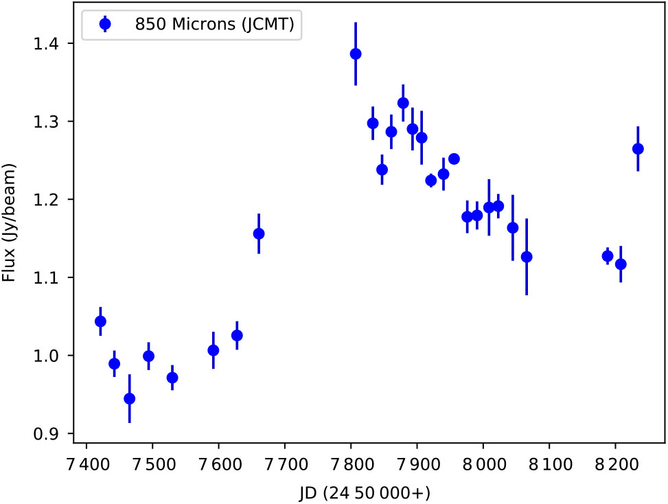
Figure 16. Time variation observed over 27 epochs at  $850\, \mu$m for the Class I YSO EC 53 in the Serpens Main star-forming region as part of the ‘JCMT Transient Survey’ (Yoo et al. Reference Yoo2017). The typical uncertainty in a single measurement is ${\sim} 20\,$mJy (S/N $\sim$ 50) and the peak-to-peak brightness variation is almost 500 mJy. Source: Figure adapted from Johnstone et al. (Reference Johnstone2018b).
Stronger variability is expected at far-IR wavelengths where Class 0 and Class I YSOs have the peak of their SEDs and the envelope emission directly scales with the internal (accretion) luminosity of the underlying protostar (Dunham et al. Reference Dunham, Crapsi, Evans, Bourke, Huard, Myers and Kauffmann2008; Johnstone et al. Reference Johnstone, Hendricks, Herczeg and Bruderer2013). At submillimeter wavelengths the emission typically scales with the envelope temperature, and thus, the far-IR signal is expected to be around four times larger such that a 10% variability in the submillimeter relates to a 40% variability in the far-IR. Contemporaneous monitoring of EC 53 in the near-IR and at 850/450 $\, \mu$m has confirmed that the longer submillimeter wavelength shows just such a diminished response to the underlying change in internal luminosity as proxied by near-IR observations (H. Yoo, private communication). Thus, carefully calibrated monitoring of protostars with SPICA should uncover a significantly larger fraction of variables than the 10% obtained by the JCMT survey.
Thanks to its high continuum sensitivity and mapping speed at wavelengths around the peak of protostellar SEDs, B-BOP, used as a total-power imager, will be ideal for monitoring hundreds of forming stars over multi-year epochs, allowing an unprecedented statistical determination of the variation in accretion on these timescales. Typical nearby deeply embedded protostars have far-IR brightnesses greater than  ${\sim}10\, $mJy, and thus, will be observed to a S/N $ \mathbin{\lower.3ex\hbox{$\buildrel>\over {\smash{\scriptstyle\sim}\vphantom{_x}}$}} $ 100 by B-BOP in a fast scanning mode. As demonstrated for ground-based submillimeter observations (Mairs et al. Reference Mairs2017a), instrument stability will need to be carefully monitored in order to achieve precise relative flux calibration of a few percent between epochs. Additional critical requirements for B-BOP will be a large, $10^5$ or higher, dynamic range and instrument robustness against extremely bright sources within the field.
Three interconnected monitoring surveys are envisioned. First, the bulk of the  ${\sim}1\,000$ nearby, Gould Belt, deeply embedded protostars will be observed every 6 months while SPICA is in orbit, requiring coverage of ${\sim} 20$ deg $^2$ (a modest 40 h of observing per epoch). This will allow for a detailed statistical characterisation of variability across multiple years. Additionally, a few carefully chosen nearby star formation fields, each roughly a square degree, will be observed weekly during their expected few month continuous observing window (for information on observing strategies for SPICA, see Roelfsema et al. Reference Roelfsema2018). For both of these nearby samples, an even larger number of Class II YSOs will be observable within each field. While these sources will be fainter at far-IR wavelengths as the emission probes the disks directly, the enhanced numbers will allow for a determination of the importance of variability throughout the evolution of a protostar. Finally, a sample of more distant high-mass star-forming regions should be observed yearly to search for rare, but extremely bright, bursts such as FU Ori events. While SPICA will not have the spatial resolution to separate individual protostars within these regions, evidence of a significant brightening can be easily followed-up with ground-based telescopes such as ALMA (see Hunter et al. Reference Hunter2017 for an example of a brightening in a high-mass star-forming region).
11. Concluding remarks
Magnetic fields are a largely unexplored ‘dimension’ of the cold Universe. While they are believed to be a key dark ingredient of the star formation process through most of Cosmic time, they remain very poorly constrained observationally, especially in the cold ISM of galaxies (e.g., Crutcher Reference Crutcher2012).
Benefiting from a cryogenic telescope, SPICA-POL or B-BOP will be 2–3 orders of magnitude more sensitive than existing or planned far-IR/submillimeter polarimeters (cf. Figure 5) and will therefore lead to a quantum step forward in the area of far-IR dust polarimetric imaging, one of the prime observational techniques to probe the topology of magnetic fields in cold, mostly neutral environments. In particular, systematic polarimetric imaging surveys of Galactic MCs and nearby galaxies with B-BOP have the potential to revolutionise our understanding of the origin and role of magnetic fields in the cold ISM of Milky-Way-like galaxies on scales from  ${\sim} 0.01\, $pc to a few kpc. The three main science drivers for B-BOP are (1) probing how magnetic fields control the formation, evolution, and fragmentation of dusty molecular filaments (Section 2), thereby setting the initial conditions for individual protostellar collapse (Sections 4 and 5); (2) characterising the structure of both turbulent and regular magnetic fields in the cold ISM of nearby galaxies, including the Milky Way, and constraining galactic dynamo models (Sections 3 and 6); and (3) testing models of dust grain alignment and informing dust physics (Section 7). Other science areas can be tackled with, or uniquely informed by, B-BOP observations, including the problem of the interaction of cosmic rays with MCs (Section 8), the study of the magnetisation of protoplanetary disks (Section 9), and the characterisation of variable accretion in embedded protostars (Section 10). Last, but not least, the leap forward provided by B-BOP in far-IR imaging polarimetry will undoubtedly lead to unexpected discoveries, such as the potential detection of polarisation from the CIB (Section 6.3).
Acknowledgments
This paper is dedicated to the memory of Bruce Swinyard, who initiated the SPICA project in Europe, but unfortunately died on 2015 May 22 at the age of 52. He was ISO-LWS calibration scientist, Herschel-SPIRE instrument scientist, first European PI of SPICA and first design lead of SAFARI. This work has received support from the European Research Council under the European Union's Seventh Framework Programme (ERC Advanced Grant Agreement no. 291294—‘ORISTARS’, and Starting Grant Agreement no. 679937—‘MagneticYSOs’). D. J. is supported by the National Research Council of Canada and by an NSERC Discovery Grant. H. B. acknowledges support from the ERC Consolidator Grant CSF-648505 and financial help from the DFG via the SFB881 ‘The Milky Way System’ (subproject B1). The National Radio Astronomy Observatory is a facility of the National Science Foundation operated under cooperative agreement by Associated Universities, Inc.


 Open access