

1 INTRODUCTION
One of the key questions facing fundamental physics and cosmology at the turn of the $21\text{st}^{\rm }$
century concerns the nature of the dark matter. Approximately 80% of the matter content of the Universe appears to be in the form of exotic, non-baryonic dark matter (cf. Planck Collaboration et al. 2013) whose clustering is believed to play a crucial role in the formation and subsequent evolution of galaxies (e.g. White & Rees Reference White and Rees1978; White & Frenk Reference White and Frenk1991). This non-baryonic dark matter is widely assumed to be cold—that is, dark matter particles were non-relativistic at the time of decoupling—and collisionless, and these properties of Cold Dark Matter (hereafter CDM) lead to a number of fundamental consequences. The first of these is that dark matter haloes have central density cusps (cf. Tremaine & Gunn Reference Tremaine and Gunn1979; Moore Reference Moore1994); the second is that the halo mass function—the number of haloes of mass M per unit mass per unit comoving volume—increases with decreasing mass as M
−α where α ~ 2.0 (cf. Table 3 of Murray et al. Reference Murray, Power and Robotham2013a) down to masses that could be as small as ~ 10 − 6M⊙ (cf. Green et al. Reference Green, Hofmann and Schwarz2004).
$21\text{st}^{\rm }$
century concerns the nature of the dark matter. Approximately 80% of the matter content of the Universe appears to be in the form of exotic, non-baryonic dark matter (cf. Planck Collaboration et al. 2013) whose clustering is believed to play a crucial role in the formation and subsequent evolution of galaxies (e.g. White & Rees Reference White and Rees1978; White & Frenk Reference White and Frenk1991). This non-baryonic dark matter is widely assumed to be cold—that is, dark matter particles were non-relativistic at the time of decoupling—and collisionless, and these properties of Cold Dark Matter (hereafter CDM) lead to a number of fundamental consequences. The first of these is that dark matter haloes have central density cusps (cf. Tremaine & Gunn Reference Tremaine and Gunn1979; Moore Reference Moore1994); the second is that the halo mass function—the number of haloes of mass M per unit mass per unit comoving volume—increases with decreasing mass as M
−α where α ~ 2.0 (cf. Table 3 of Murray et al. Reference Murray, Power and Robotham2013a) down to masses that could be as small as ~ 10 − 6M⊙ (cf. Green et al. Reference Green, Hofmann and Schwarz2004).
Based on the results of cosmological N-body simulations, cuspy haloes and an abundance of small-scale structure—low-mass haloes and subhaloes—are now well established as robust predictions of the CDM model (e.g. Springel et al. Reference Springel2008). If we consider a Universe in which low-mass halo and subhalo formation is suppressed, as in Warm Dark Matter (hereafter WDM) models, we find that haloes can form cores (albeit small ones; cf. Villaescusa-Navarro & Dalal Reference Villaescusa-Navarro and Dalal2011) but they are likely to remain cuspy for plausible WDM particle masses (m WDM ≳ 0.5 − 2keV), even when free streaming is accounted for (e.g. Colín et al. Reference Colín, Valenzuela and Avila-Reese2008; Macciò et al. Reference Macciò, Paduroiu, Anderhalden, Schneider and Moore2012). In contrast, we expect the abundance and clustering of low-mass haloes to be suppressed in WDM models (e.g. Dunstan et al. Reference Dunstan, Abazajian, Polisensky and Ricotti2011; Smith & Markovic Reference Smith and Markovic2011; Schneider et al. Reference Schneider, Smith and Reed2013; Benson et al. Reference Benson2013; Pacucci et al. Reference Pacucci, Mesinger and Haiman2013), and so it can be argued that it is the abundance of small-scale structure, rather than central density cusps, that is the defining characteristic of the CDM modelFootnote 1 .
However, we expect few of these low-mass haloes to host galaxies because galaxy formation will be inefficient in their shallow potential wells (e.g. Dekel & Silk Reference Dekel and Silk1986; Efstathiou Reference Efstathiou1992; Thoul & Weinberg Reference Thoul and Weinberg1996; Benson et al. Reference Benson, Lacey, Baugh, Cole and Frenk2002). For example, supernovae (e.g. Dekel & Silk Reference Dekel and Silk1986) and photo-ionising sources (e.g. Benson et al. Reference Benson, Lacey, Baugh, Cole and Frenk2002; Cantalupo Reference Cantalupo2010) can quench galaxy formation in low-mass haloes, while the likelihood that a low-mass halo hosts a satellite galaxy appears to be stochastic (cf. Boylan-Kolchin et al. Reference Boylan-Kolchin, Bullock and Kaplinghat2012; Garrison-Kimmel et al. Reference Garrison-Kimmel, Rocha, Boylan-Kolchin, Bullock and Lally2013), suggesting that the process is highly sensitive to details of a galaxy's assembly history (i.e. environment, gas accretion and star formation history, etc.–.–.). This raises the question, if low-mass haloes and subhaloes remain dark because galaxy formation is inefficient on these mass scales, how can we tell the difference between a Universe in which small-scale structure is present but dark and one in which its formation is suppressed, as in WDM models?
In this paper, we use the results of cosmological N-body simulations to address this question, comparing systematically dark matter halo properties in a fiducial ΛCDM cosmology and in ΛWDM-like dark matter models, in which low-mass halo formation is suppressed by truncating the ΛCDM power spectrum on small scales. Numerous studies have investigated the halo mass function in WDM models (recent examples include Schneider et al. Reference Schneider, Smith, Maccio and Moore2012, Reference Schneider, Smith and Reed2013; Pacucci et al. Reference Pacucci, Mesinger and Haiman2013; Benson et al. Reference Benson2013) and associated issues arising from discreteness effects in such simulations (e.g. Wang & White Reference Wang and White2007; Schneider et al. Reference Schneider, Smith and Reed2013; Angulo et al. Reference Angulo, Hahn and Abel2013; Hahn et al. Reference Hahn, Abel and Kaehler2013), but we note that direct measurement of the halo mass function observationally is fraught with difficulty (cf. Murray et al. Reference Murray, Power and Robotham2013b). For this reason, we focus on three measures of the halo population that are potentially accessible to observation—(i) the spatial clustering of low-mass haloes around galaxy- and group-mass haloes (1011 h −1M⊙≲ M vir≲ 1013 h −1M⊙); (ii) the rate at which these haloes assemble their mass and at which they experience mergers; and (iii) their angular momentum content. Although we analyse properties of the halo population, we reason that they provide a baseline for trends that we observe in the galaxy population.
We choose the cut-off mass M cut, the mass scale below which halo formation is suppressed, to vary between 5×10⁹ h −1M⊙≲M cut≲1011 h −1M⊙. These values of M cut are unrealistic in the sense that they are too large to be consistent with observational constraints (see, for example, the review of Primack Reference Primack and Cline2009, assuming corresponding filtering masses from Bode et al. Reference Bode, Ostriker and Turok2001) but they allow us to experiment with the consequences of progressively more aggressive truncations of the initial power spectrum on the properties of haloes with M ≳ 1011M⊙.
The structure of this paper is as follows. In Section 2, we describe our simulations, detailing how we set them up, and summarising our approach to constructing merger trees and halo sample selection. In Section 3, we focus on the spatial clustering of haloes and demonstrate that the clustering strength of low-mass haloes is suppressed relative to the ΛCDM model in our truncated models. We show how this suppression in clustering impacts the number and frequency of minor mergers (Section 4) and we explore measures of halo angular momentum and spin (Section 5). Finally, in Section 6 we summarise our results, assessing their implications for developing robust astrophysical tests of the nature of the dark matter.
2 THE SIMULATIONS
We have run a sequence of cosmological N-body simulations that follow the formation and evolution of dark matter haloes in a box of side 20h − 1Mpc from a starting redshift of z = 100 to z = 0. For each run, we assume a flat cosmology with a dark energy term, and for convenience we adopt the cosmological parameters of Spergel (Reference Spergel2007)—matter and dark energy density parameters of Ωm = 0.24 and ΩΛ = 0.76, a dimensionless Hubble parameter of h = 0.73, a normalisation of σ8 = 0.74, and a primordial spectral index of n spec = 0.95. Each simulation volume contains 2563 equal-mass particles, which for the adopted cosmological parameters gives particle masses of m p = 3.176 × 10⁷ h − 1M⊙.
The respective runs differ in the spatial scale below which small-scale power in the initial conditions is suppressed. We generate a single realisation of the ΛCDM power spectrum appropriate for our choice of cosmological parameters and in the case of the truncated models we introduce a sharp cut-off in the ΛCDM power spectrum at progressively larger spatial scales. This cut-off spatial scale is set by the mass scale below which we wish to suppress halo formation. Details about the truncated models are given in the next section.
All of our simulations were run using the parallel TreePM code gadget2 (Springel Reference Springel2005) with a constant comoving gravitational softening ε = 1.5h
− 1kpc and individual and adaptive particle time-steps. These were assigned according to the criterion $\Delta t = \eta \sqrt{\epsilon /a}$
, where a is the magnitude of a particle's gravitational acceleration and η = 0.05 determines the accuracy of the time integration.
$\Delta t = \eta \sqrt{\epsilon /a}$
, where a is the magnitude of a particle's gravitational acceleration and η = 0.05 determines the accuracy of the time integration.
2.1 Truncated dark matter models
2.1.1 Truncating the initial power spectrum
We are interested in models in which small-scale power is suppressed at early times. Physically suppression arises because dark matter free streams, which acts as a damping mechanism to wash out primordial density perturbations and to introduce a cut-off in the linear matter power spectrum. If the dark matter particle is a thermal relic, the spatial scale at which this cut-off occurs can be calculated (cf. Bergström Reference Bergström2000). The free streaming scale λfs can be expressed as
 \begin{equation}
\lambda _{\rm fs} = 0.2\,(\Omega _{\rm dm}\,h^2)^{1/3}\,\left(\frac{m_{\rm dm}}{{\rm keV}}\right)^{-4/3} \,\rm Mpc,
\end{equation}
\begin{equation}
\lambda _{\rm fs} = 0.2\,(\Omega _{\rm dm}\,h^2)^{1/3}\,\left(\frac{m_{\rm dm}}{{\rm keV}}\right)^{-4/3} \,\rm Mpc,
\end{equation}
where m dm is the dark matter particle mass measured in keV and Ωdm is the dark matter density (cf. Boehm et al. Reference Boehm, Mathis, Devriendt and Silk2005).
Provided λfs is small compared to the spatial scales we are interested in simulating, the power spectrum will differ little from the ΛCDM power spectrum (which itself may have a cut-off on comoving scales of order 1 pc; cf. Green et al. Reference Green, Hofmann and Schwarz2004). However, as λfs increases and approaches the scale that we wish to resolve, then it becomes necessary to determine how the power spectrum changes. The shape of the linear power spectrum for collisionless WDM models has been calculated by a number of authors (e.g. Bardeen et al. Reference Bardeen, Bond, Kaiser and Szalay1986; Bode et al. Reference Bode, Ostriker and Turok2001), and it can be recovered from the CDM power spectrum by introducing an exponential cut-off at small scales. The larger λfs, the larger the mass scale Mfs below which structure formation is suppressed and the smaller the wave-number k at which the WDM and CDM power spectra differ, although the relationship between λfs and Mfs is sensitive to the precise nature of the WDM particle.
We do not wish to make any assumptions about the precise nature of the dark matter other than that it is collisionless and that low-mass halo formation is suppressed, and so we follow Moore et al. (Reference Moore, Quinn, Governato, Stadel and Lake1999) and truncate sharply the power spectrum at k cut, suppressing power at wave-numbers k≥k cut. We choose k cut by identifying a mass scale M cut and estimating the comoving length scale R cut,
 \begin{equation}
R_{\rm cut} = \left(\frac{3\,M_{\rm cut}}{4\pi }\frac{1}{\overline{\rho }}\right)^{1/3},
\end{equation}
\begin{equation}
R_{\rm cut} = \left(\frac{3\,M_{\rm cut}}{4\pi }\frac{1}{\overline{\rho }}\right)^{1/3},
\end{equation}
where $\overline{\rho }$
is the mean density of the Universe.
$\overline{\rho }$
is the mean density of the Universe.
2.1.2 Modelling free streaming
Similarly, we choose not to include the effect of free streaming in our initial conditions—partly because we wish to avoid assumptions about the precise nature of the dark matter, and partly for pragmatic reasons, which we now explain. In practice, free streaming is mimicked by assigning a random velocity component (typically drawn from a Fermi-Dirac distribution) to particles in addition to their velocities predicted by linear theory (cf. Klypin et al. Reference Klypin, Holtzman, Primack and Regos1993; Colín et al. Reference Colín, Valenzuela and Avila-Reese2008; Macciò et al. Reference Macciò, Paduroiu, Anderhalden, Schneider and Moore2012). However, capturing this effect correctly in a N-body simulation is difficult—it can lead to an unphysical excess of small-scale power in the initial conditions if the simulation is started too early (see Figure 1 of Colín et al. Reference Colín, Valenzuela and Avila-Reese2008 for a nice illustration of this problem).

Figure 1. The projected density distribution in 2h − 1Mpc slices taken through the centres of each of the boxes. We have smoothed the particle mass using an adaptive Gaussian kernel and projected onto a mesh. Each mesh point is weighted according to the logarithm of its projected surface density, and so the ‘darker’ the mesh point, the higher the projected surface density.
Precisely, how early is too early has yet to be properly quantified, but it will depend explicitly on dark matter particle mass—the lower the mass, the longer the free streaming scale, and the larger the random velocity component required. If this exceeds the typical velocity predicted by linear theory, a population of spurious haloes forms (e.g. Klypin et al. Reference Klypin, Holtzman, Primack and Regos1993) that can exceed in number by factors of ~ 10 the population that forms when no random velocity component is included, as studied by Wang and White (Reference Wang and White2007). This is unlikely to be a problem for studying the mass profiles of haloes—for example, Colín et al. (Reference Colín, Valenzuela and Avila-Reese2008) started their simulations at reasonably late times because the random velocity component damps away with decreasing redshift while the velocities predicted by linear theory increase—but it is not clear how much of a problem it will be for our study, in which we study quantities that depend on spatial correlations between haloes. For this reason, we do not include the effect of free streaming, deferring this to a forthcoming study on discreteness effects in WDM-like simulations (C. Power et al., in preparation).
2.1.3 Generation of initial conditions
We follow the standard procedure (e.g. Power et al. Reference Power, Navarro, Jenkins, Frenk, White, Springel, Stadel and Quinn2003) of generating a statistical realisation of the high redshift density field using the appropriate linear theory power spectrum, from which initial displacements and velocities are computed and imposed on a suitable uniform particle load; for this study we adopt an initial glass distribution (cf. White Reference White1994). We use the Boltzmann code cmbfast (Seljak & Zaldarriaga Reference Seljak and Zaldarriaga1996) to generate the CDM transfer function for our choice of cosmological parameters. This is convolved with the primordial power spectrum (P(k)∝kn , where n is the primordial spectral index) to obtain the appropriate ΛCDM power spectrum P(k). To obtain a truncated model, we chop P(k) sharply at k cut = 2π/R cut (where R cut is given by Equation (2)) and thereby suppress power on scales k≳k cut.
We consider five cases—a fiducial ΛCDM model and truncated models in which small-scale power is suppressed at masses below M
cut = 5×10⁹, 1010, 5×10¹⁰ and $10^{11} h^{-1} \text{M}_{\odot ,}$
respectively. Note that the cut-off wave-number k
cut is always less than the Nyquist frequency of the simulation, k
Ny ≃ 40hMpc − 1. Values for the cut-off masses and wave-numbers are given in Table 1.
$10^{11} h^{-1} \text{M}_{\odot ,}$
respectively. Note that the cut-off wave-number k
cut is always less than the Nyquist frequency of the simulation, k
Ny ≃ 40hMpc − 1. Values for the cut-off masses and wave-numbers are given in Table 1.
Table 1 Truncated models: simulation details.
2.2 Halo identification and merger trees
2.2.1 Halo identification
Groups are identified using AMIGA's Halo Finder (AHF) (cf. Knollmann & Knebe Reference Knollmann and Knebe2009). AHF locates groups as peaks in an adaptively smoothed density field using a hierarchy of grids and a refinement criterion that is comparable to the force resolution of the simulation. Local potential minima are calculated for each of these peaks and the set of particles that are gravitationally bound to the peaks are identified as the groups that form our halo catalogue. Each halo in the catalogue is then processed, producing a range of structural and kinematic information.
We adopt the standard definition of a halo such that the virial mass is
 \begin{equation}
M_{\rm vir}=4 \pi \rho _{\rm crit} \Delta _{\rm vir} r_{\rm vir}^3/3,
\end{equation}
\begin{equation}
M_{\rm vir}=4 \pi \rho _{\rm crit} \Delta _{\rm vir} r_{\rm vir}^3/3,
\end{equation}
where $\rho _{\text{crit}}=3H^2/8\pi G$
is the critical density of the Universe and r
vir is the virial radius, which defines the radial extent of the halo. The virial over-density criterion, Δvir, is a multiple of the critical density, and corresponds to the mean over-density at the time of virialisation in the spherical collapse model (the simplest analytic model of halo formation; cf. Eke et al. Reference Eke, Cole and Frenk1996). In an Einstein-de Sitter Universe, Δvir≃178, while in the favoured ΛCDM model Δvir≃92 at z = 0.
$\rho _{\text{crit}}=3H^2/8\pi G$
is the critical density of the Universe and r
vir is the virial radius, which defines the radial extent of the halo. The virial over-density criterion, Δvir, is a multiple of the critical density, and corresponds to the mean over-density at the time of virialisation in the spherical collapse model (the simplest analytic model of halo formation; cf. Eke et al. Reference Eke, Cole and Frenk1996). In an Einstein-de Sitter Universe, Δvir≃178, while in the favoured ΛCDM model Δvir≃92 at z = 0.
Defined in this way, the virial radius r vir provides a convenient albeit approximate boundary for a dark matter halo that can be estimated easily from simulation data. However, it is only approximate—haloes that form in cosmological simulations are relatively complex structures. They are generally aspherical (e.g. Bailin & Steinmetz Reference Bailin and Steinmetz2005) and asymmetric (e.g. Gao & White Reference Gao and White2006) with no simple boundary (e.g. Prada et al. Reference Prada, Klypin, Simonneau, Betancort-Rijo, Patiri, Gottlöber and Sanchez-Conde2006), and so defining an appropriate boundary is not straightforward. This presents difficulties when calculating, for example, a halo's angular momentum and its binding energy (cf. Łokas & Mamon Reference Łokas and Mamon2001). Material bound to the halo can lie outside of r vir, and this will distort the angular momentum and binding energy one measures for the halo using only material from within r vir. This issue has been touched on by previous authors (e.g. Cole & Lacey Reference Cole and Lacey1996; Łokas & Mamon Reference Łokas and Mamon2001; Shaw et al. Reference Shaw, Weller, Ostriker and Bode2006; Power et al. Reference Power, Knebe and Knollmann2012) in the context of identifying when a halo is in virial equilibrium. In a similar vein, the angular momentum one measures using only material from within r vir will be biased. This is an important caveat that we need to bear in mind when discussing our analysis of halo angular momentum in Section 5.
2.2.2 Halo merger trees
Halo merger trees are constructed by linking halo particles at consecutive output times.
-
• For each pair of group catalogues constructed at consecutive output times t 1 and t 2>t 1, the ‘ancestors’ of ‘descendant’ groups are identified. For each descendent identified in the catalogue at the later time t 2, we sweep over its associated particles and locate every ancestor at the earlier time t 1 that contains a subset of these particles. A record of all ancestors at t 1 that contain particles associated with the descendent at t 2 is maintained.
-
• The ancestor at time t 1 that contains in excess of f prog of these particles and also contains the most bound particle of the descendent at t 2 is deemed the main progenitor. Typically f prog = 0.5, i.e. the main progenitor contains in excess of half the final mass.
Each group is then treated as a node in a tree structure, which can be traversed either forwards, allowing one to identify a halo at some early time and follow it forward through the merging hierarchy, or backwards, allowing one to identify a halo and all its progenitors at earlier times. In our analysis, we concentrate on the main trunk of the merger tree, in which we follow the evolution of the main progenitor of a halo to earlier times.
2.3 Selecting the halo sample
However, care must be taken when including haloes with masses below M cut in any analysis. An unfortunate feature of simulations of cosmologies in which small-scale power is suppressed at early times is the formation of unphysical low-mass haloes by the fragmentation of filaments, driven by the discreteness of the matter distribution. These spurious haloes form preferentially in filaments, at regular intervals of order the mean interparticle separation of the simulation, akin to ‘beads on a string’ (see below). The mass scale below which these spurious ‘haloes’ form can be estimated from the halo mass function as a sharp upturn in the number density, and it has been shown to scale as M lim ~ 3.9 m 1/3 p M cut 2/3, where mp is the particle mass (Wang & White Reference Wang and White2007).
We wish to identify haloes in the truncated models that have clearly identifiable counterparts in the fiducial ΛCDM simulation. These haloes form the halo sample upon which our analysis is based. By selecting haloes in this way, we can track the merger trees of the counterparts and study the merging and accretion histories of individual systems, correlating any differences in halo properties with the details of their mass assembly. We can also avoid including in our analysis spurious (unphysical) haloes that form below the mass cut-off in the truncated models (see, for example, Wang & White Reference Wang and White2007).
To identify counterparts, we adapt our algorithm for linking haloes across time slices when building merger trees to link haloes between runs at a given time.
-
• For each pair of group catalogues, we process each group and compute ‘virial’ quantities, namely the virial mass and radius, and the set of particles that belong to each halo.
-
• For each halo in the fiducial ΛCDM model at time t, we loop over its associated particles and determine how many of these particles are present in haloes in the corresponding truncated model catalogue.
-
• The halo in the truncated model that contains in excess of f count = 75% of these particles is identified as a counterpart candidate. However, the candidate halo can be part of a much larger structure in the fiducial ΛCDM model, so we also require that the mass of the candidate halo not differ from its CDM counterpart by not more than a factor of 25%. Haloes that satisfy these conditions are identified as counterparts.
3 SPATIAL CLUSTERING
As our starting point, we compare and contrast the spatial clustering of dark matter haloes in the ΛCDM and truncated models respectively as a function of redshift. We expect differences between models to be apparent for haloes with masses M ~ M cut and to become more pronounced with increasing redshift, when M cut is a larger fraction of the typical collapsing mass M*.
3.1 Visual impression
In Figure 1, we show the projected dark matter distribution in thin slices (20 × 20 × 2h − 3Mpc3) taken through the ΛCDM (upper panels), Truncated B (middle panels; hereafter TruncB), and D (lower panels; hereafter TruncD) at z = 0, 1, and 4 (from left to right). Each slice is centred on the geometric centre of the simulation volume and the grey scale is weighted by the logarithm of projected density.
Figure 1 is instructive because it provides a powerful visual impression of the effect of suppressing small-scale power at early times. The filamentary network is largely unaffected and the positions of the most massive haloes, which form at the nodes of these filaments, are similar in each of the models we have looked at. What is striking, however, is the impact on the abundance of low-mass haloes, which appear as small dense knots in projection. As M cut increases, the projected number density of these low-mass haloes decreases markedly as we go from the ΛCDM run to the TruncD run (top and bottom panels, respectively). This is evident in the clustering around more massive haloes and the absence of low-mass systems in the void regions. Furthermore, the contrast between the models becomes increasingly noticeable with increasing redshift—compare z = 0 and z = 4. Note also the presence of the low-mass haloes distributed along filaments in ‘beads-on-a-string’ fashion in the truncated models.
3.2 Spatial clustering
In Figure 2, we investigate how the clustering strength of haloes differs between the different dark matter models and as a function of redshift. We quantify clustering strength by the correlation function ξ(r), which measures the excess probability over random that a pair of haloes i and j will be separated by a distance $r=|\vec{r}|=|\vec{r}_i-\vec{r}_j|$
. ξ(r) is estimated using
$r=|\vec{r}|=|\vec{r}_i-\vec{r}_j|$
. ξ(r) is estimated using
 \begin{equation}
\xi (r)=1+\frac{\overline{DD(r)}}{\overline{RR(r)}},
\end{equation}
\begin{equation}
\xi (r)=1+\frac{\overline{DD(r)}}{\overline{RR(r)}},
\end{equation}
where $\overline{DD(r)}$
is the number of haloes at comoving separation r compared to the number in a random distribution
$\overline{DD(r)}$
is the number of haloes at comoving separation r compared to the number in a random distribution $\overline{RR(r)}$
. Because our focus is on differences, we construct the ratio of
$\overline{RR(r)}$
. Because our focus is on differences, we construct the ratio of $N(r)=\overline{DD(r)}=\overline{RR(r)}(\xi (r)-1)$
for each truncated model to N(r)CDM for the fiducial ΛCDM run.
$N(r)=\overline{DD(r)}=\overline{RR(r)}(\xi (r)-1)$
for each truncated model to N(r)CDM for the fiducial ΛCDM run.

Figure 2. Evolution of spatial clustering with redshift. We examine how the clustering strength of haloes with respect to the fiducial ΛCDM model varies across the runs TruncA (solid curves), TruncB (short-dashed curves), TruncC (long-dashed curves), and TruncD (dotted-dashed curves) at z = 0, 1, 2, and 3 by plotting the ratio N(r)/N(r)CDM—the number of haloes with comoving halo separation r—as a function of r. In the upper panel, we look at the clustering of all secondary haloes with mass M vir ⩾ 3 × 10⁹ h − 1M⊙ around primary haloes with mass M vir ⩾ 1011 h − 1M⊙, while in the lower panel we look at the clustering of only massive haloes, for which both the primary and secondary masses are M vir ⩾ 1011 h − 1M⊙.
In the upper panel of Figure 2, we consider pairs of haloes in which the primary's mass is M vir ⩾ 1011 h − 1M⊙ and the secondary's mass is M vir ⩾ 3 × 10⁹ h − 1M⊙, while in the lower panel, we consider pairs of haloes in which both the primary and secondary masses M vir ⩾ 1011 h − 1M⊙. This reveals that the clustering strength of low-mass haloes around high-mass haloes (i.e. M vir ⩾ 1011 h − 1M⊙) decreases with increasing M cut, although the dependence on M cut does not appear to be straightforward. In the TruncA and TruncB runs, we find that N(r)/N(r)CDM is close to unity out to r ≃ 10h − 1Mpc, never deviating by more than 10% to within ~ 500h − 1kpc at all redshifts. For the TruncC and TruncD runs, the suppression in clustering strength is quite marked—by ~40% for the TruncC run and ~50% for the TruncD run. Large deviations at small radii reflect the small numbers of very close pairs. In contrast, the clustering strength of massive haloes (i.e. M ⩾ 1011 h − 1M⊙) does not appear to be affected by M cut, as we inferred from Figure 1. The ratio N(r)/N(r)CDM is noisy—reflecting the lower number density of massive haloes—but it is approximately unity between 0≲z≲3.
4 MASS ACCRETION AND MERGING HISTORIES
Suppressing small-scale power at early times leads to a reduction in the clustering of low-mass haloes around massive haloes (M vir ≳ 1011 h − 1M⊙) at z≲3, which implies that the number of likely minor mergers a typical halo will experience during a given period should decline with increasing M cut. We expect this to depend on both halo mass and epoch. At a given z, the merging history of haloes with masses M vir~M cut should be more sensitive to the clustering of small-scale structure than haloes with masses M vir≫M cut. Similarly, at earlier times when the typical collapsing mass M* is smaller and M cut is a larger fraction of M*, we would expect the effect of suppressing small-scale structure to be more pronounced.
When computing mass accretion and merging rates, we use merger trees for all haloes between 5 × 10¹⁰ h − 1M⊙ (~1 600 particles) and 1013 h − 1M⊙ at z = 0. Note that we have a hard lower limit of 100 particles for a halo to be retained in our catalogues; this corresponds to a mass of ~ 3.2 × 10⁹ h − 1M⊙, and so we cannot identify minor mergers with mass ratios of less than ~6% in our most poorly resolved haloes.
4.1 Mass accretion rate
In Figure 3, we show how the mass accretion rate of the most massive progenitors of haloes identified at z = 0 evolves with redshift. Note that his accretion rate includes both smooth accretion and minor and major mergers. The distinction between minor mergers and smooth accretion may be a moot one in the CDM model—as the mass and force resolution of the simulation increases, we continue to resolve increasing numbers of low-mass haloes—but this is not necessarily the case in the truncated models that we consider.

Figure 3. Impact on mass accretion rate. For each halo at z = 0, we follow the main branch of its merger tree to higher redshifts and compute the difference in virial mass between progenitors at z
0 and z
1>z
0. From this, we compute the mass accretion rate with respect to time (in Gyrs), normalised by the virial mass of the descendent halo at z= 0. Within each of the mass bins, we compute the average mass accretion rate for haloes in the fiducial λCDM run (red-filled circles), TruncB ( $M_{\rm cut}=10^{10} h^{-1} \text{M}_{\odot }$
; green-filled squares), TruncC (
$M_{\rm cut}=10^{10} h^{-1} \text{M}_{\odot }$
; green-filled squares), TruncC ( $M_{\rm cut}=5 \times 10^{10} h^{-1} \text{M}_{\odot }$
; cyan-filled triangles), and TruncD (
$M_{\rm cut}=5 \times 10^{10} h^{-1} \text{M}_{\odot }$
; cyan-filled triangles), and TruncD ( $M_{\rm cut}=10^{11} h^{-1} \text{M}_{\odot }$
; magenta crosses).
$M_{\rm cut}=10^{11} h^{-1} \text{M}_{\odot }$
; magenta crosses).
From upper to lower panels, we show the average accretion rate as a function of redshift for haloes with virial masses at z = 0 in the range 5 × 10¹⁰ ⩽ M
vir/h
− 1M⊙ ⩽ 1011 (filled circles), $10^{11} \leqslant \rm M_{\rm vir}/h^{-1} \rm M_{\odot } \leqslant 5 \times 10^{11}$
(filled squares), 5 × 10¹¹ ⩽ M
vir/h
− 1M⊙ ⩽ 1012 (filled triangles), and M
vir/h
− 1M⊙ ⩽ 1012 (crosses). Note that we measure the accretion rate as the change in virial mass (ΔM) per unit redshift (Δz) per unit time (Δt), normalised by the final (i.e. z=0) virial mass. Bars indicate r.m.s. scatter.
$10^{11} \leqslant \rm M_{\rm vir}/h^{-1} \rm M_{\odot } \leqslant 5 \times 10^{11}$
(filled squares), 5 × 10¹¹ ⩽ M
vir/h
− 1M⊙ ⩽ 1012 (filled triangles), and M
vir/h
− 1M⊙ ⩽ 1012 (crosses). Note that we measure the accretion rate as the change in virial mass (ΔM) per unit redshift (Δz) per unit time (Δt), normalised by the final (i.e. z=0) virial mass. Bars indicate r.m.s. scatter.
Figure 3 shows that haloes accrete their mass at similar rates across the different models, regardless of whether or not small-scale power is suppressed at early times. On average, less massive haloes tend to have higher accretion rates at z≳1 than their more massive counterparts, but this rate starts to drop z ~ 1 and declines steadily to z = 0 (see also Figure 9 for detailed mass accretion histories for individual haloes). In contrast, more massive haloes accrete their mass at a steady rate. We find that our accretion rates for ΛCDM haloes are in good agreement with those consistent with those of, for example, Maulbetsch et al. (Reference Maulbetsch, Avila-Reese, Colín, Gottlöber, Khalatyan and Steinmetz2007).
4.2 Merger rates
In Figure 4, we focus on the merger rate ΔN/Δz/Δt and its variation with redshift, where ΔN is the number of mergers per unit redshift per unit time. Here, differences between runs are immediately apparent and in the sense that we expect—for halo masses close to M
cut increases, the merging rate decreases. Note that the estimated merger rate is quite noisy in the lowest mass bin (upper panel), especially at early times—in this case, the lower limit of 100 particles imposed by our halo catalogues corresponds to a merger of progressively greater mass ratio with increasing redshift. For this reason, we focus on haloes with masses at z = 0 in excess of $10^{11} h^{-1} \text{M}_{\odot }$
. For haloes with masses between 1011 ⩽ M
vir/h
− 1M⊙ ⩽ 5 × 10¹¹, we find that the average merger rate in the TruncC (TruncD) model is a factor of ~3(1.5) smaller than that in the fiducial ΛCDM model, and this is approximately constant with redshift. The difference is less pronounced for haloes with masses between 5 × 10¹¹ ⩽ M
vir/h
− 1M⊙ ⩽ 1012, and for haloes with masses in excess of 1012
h
− 1M⊙ there is no discernible difference in the merging rates with redshift.
$10^{11} h^{-1} \text{M}_{\odot }$
. For haloes with masses between 1011 ⩽ M
vir/h
− 1M⊙ ⩽ 5 × 10¹¹, we find that the average merger rate in the TruncC (TruncD) model is a factor of ~3(1.5) smaller than that in the fiducial ΛCDM model, and this is approximately constant with redshift. The difference is less pronounced for haloes with masses between 5 × 10¹¹ ⩽ M
vir/h
− 1M⊙ ⩽ 1012, and for haloes with masses in excess of 1012
h
− 1M⊙ there is no discernible difference in the merging rates with redshift.

Figure 4. Impact on merger rate. For each halo at z = 0, we follow the main branch of its merger tree to higher redshifts and determine the number of mergers with mass ratios in excess of 6% experienced by the halo between z 0 and z 1>z 0. From this, we compute the merger rate per unit redshift per unit time. Within each of the mass bins, we compute the average merger rate for haloes in the fiducial λCDM run (red-filled circles), TruncB (M cut = 1010 h − 1M⊙; green-filled squares), TruncC (M cut = 5 × 10¹⁰ h − 1M⊙; cyan-filled triangles), and TruncD (M cut = 1011 h − 1M⊙; magenta crosses).
In Figure 5, we assess how major mergers are affected by suppression of small-scale power at early times. This demonstrates that the likelihood that the mass ratio of the most significant merger experienced by a halo since z≃0.5 does not depend strongly on whether or not small-scale structure has been suppressed. Here, we follow Power et al. (Reference Power, Knebe and Knollmann2012) and compute the distribution of the most significant merger δmax = M acc/M vir experienced by each halo (identified at z = 0) since ~0.5Footnote 2 , split according to virial mass at z=0.

Figure 5. Distribution of most significant mergers. For each halo at z=0, we compute the mass ratio of the most significant merger δmax that it has experienced since z≃0.5 and construct the frequency distribution of δmax for the respective models.
There are a number of interesting trends in this figure. The first is that most significant mergers with large mass ratios (i.e. minor mergers) are relatively uncommon; the probability distribution increases approximately as a power law with δmax as δ1.2 max. The second is that, in the CDM model, the likelihood that a halo experiences a most significant merger with a given δmax does not depend strongly on its mass. For example, a halo with virial mass of 1011 h − 1M⊙ is as likely to have experienced a major merger with mass ratio of ~50% as a 1013 h −1 M ⊙ halo—approximately 20%. The third is that there is some evidence that haloes in the mass range 5 × 10¹⁰ ⩽ M vir/h − 1M⊙ ⩽ 1011 are less likely to experience major mergers with mass ratios in excess of ~50% (compare TruncB and TruncD).
5 ANGULAR MOMENTUM CONTENT
Suppressing small-scale power at early times impacts both the clustering strength of low-mass haloes and the rate of mergers and accretions at later times. Do we see a corresponding influence on the angular momentum content of haloes at later times?
5.1 Spin parameter
We begin by considering the spin parameter λ, which quantifies the degree to which the halo is supported by rotation and which we define using the ‘classical’ definition of Peebles (Reference Peebles1969),
 \begin{equation}
{\lambda = \frac{J|E|^{1/2}}{GM_{\rm vir}^{5/2}}.}
\end{equation}
\begin{equation}
{\lambda = \frac{J|E|^{1/2}}{GM_{\rm vir}^{5/2}}.}
\end{equation}
Here J and E are the total angular momentum and binding energy respectively of material with r vir and G is the gravitational constant. We impose a lower limit of 600 particles within r vir (M vir ⩾ 2 × 10¹⁰ h − 1M⊙) when measuring λ; this ensures that both J and E are unaffected by discreteness effects (cf. Power et al. Reference Power, Knebe and Knollmann2012).
In Figure 6, we show how the median spin of the halo population evolves with redshift. In the upper panel, we focus on the haloes with $M_{\rm vir} \geqslant 2 \times 10^{10} h^{-1} \text{M}_{\odot }$
, while in the lower panel we consider haloes with
$M_{\rm vir} \geqslant 2 \times 10^{10} h^{-1} \text{M}_{\odot }$
, while in the lower panel we consider haloes with $M_{\rm vir} \geqslant 10^{11} h^{-1} \text{M}_{\odot }$
. Filled circles, squares, triangles, and crosses represent the median spin of the halo populations in the ΛCDM, TruncB, TruncC, and TruncD runs, and error bars indicate the 25th and 75th percentiles of the distribution. This figure suggests that the behaviour of the distribution of λ is sensitive to M
cut—systematic differences are apparent in the TruncC and TruncD runs when we include all haloes with
$M_{\rm vir} \geqslant 10^{11} h^{-1} \text{M}_{\odot }$
. Filled circles, squares, triangles, and crosses represent the median spin of the halo populations in the ΛCDM, TruncB, TruncC, and TruncD runs, and error bars indicate the 25th and 75th percentiles of the distribution. This figure suggests that the behaviour of the distribution of λ is sensitive to M
cut—systematic differences are apparent in the TruncC and TruncD runs when we include all haloes with $M_{\rm vir} \geqslant 2 \times 10^{10} h^{-1} \text{M}_{\odot }$
, whereas the distributions are statistically similar when we include only haloes with
$M_{\rm vir} \geqslant 2 \times 10^{10} h^{-1} \text{M}_{\odot }$
, whereas the distributions are statistically similar when we include only haloes with $M_{\rm vir} \geqslant 10^{11} h^{-1} \text{M}_{\odot }$
.
$M_{\rm vir} \geqslant 10^{11} h^{-1} \text{M}_{\odot }$
.

Figure 6. Variation of median λ with redshift. We show how the median spin parameter λmed varies with redshift. In the left-hand panel, we consider all haloes with virial masses in excess of $M_{\rm vir} \geqslant 1.9 \times 10^{10} h^{-1} \text{M}_{\odot }$
, while in the right-hand panel, we consider all haloes that satisfy
$M_{\rm vir} \geqslant 1.9 \times 10^{10} h^{-1} \text{M}_{\odot }$
, while in the right-hand panel, we consider all haloes that satisfy $M_{\rm vir} \geqslant 10^{11} h^{-1} \text{M}_{\odot }$
. Lower and upper error bars represent the
$M_{\rm vir} \geqslant 10^{11} h^{-1} \text{M}_{\odot }$
. Lower and upper error bars represent the $25\text{th}^{\rm }$
and
$25\text{th}^{\rm }$
and $75\text{th} ^{\rm }$
percentiles. The filled circles, squares, triangles, and crosses correspond to the fiducial ΛCDM, TruncB, TruncC, and TruncD runs, respectively.
$75\text{th} ^{\rm }$
percentiles. The filled circles, squares, triangles, and crosses correspond to the fiducial ΛCDM, TruncB, TruncC, and TruncD runs, respectively.
This figure is interesting because we include a large population of haloes in the TruncC and TruncD runs with M
vir≤M
cut when we include haloes with $M_{\rm vir} \geqslant 2 \times 10^{10} h^{-1} \text{M}_{\odot }$
, and so the apparent differences are to be expected. In contrast, we do not see any evident differences when we include haloes with
$M_{\rm vir} \geqslant 2 \times 10^{10} h^{-1} \text{M}_{\odot }$
, and so the apparent differences are to be expected. In contrast, we do not see any evident differences when we include haloes with $M_{\rm vir} \geqslant 10^{11} h^{-1} \text{M}_{\odot }$
. This is also interesting because it reveals that the median λ increases with decreasing redshift at approximately the same rate—in proportion to (1 + z)−0.3—regardless of whether or not we include haloes with masses below M
cut.
$M_{\rm vir} \geqslant 10^{11} h^{-1} \text{M}_{\odot }$
. This is also interesting because it reveals that the median λ increases with decreasing redshift at approximately the same rate—in proportion to (1 + z)−0.3—regardless of whether or not we include haloes with masses below M
cut.
In Figure 7, we focus on individual haloes, showing how λ and the specific angular momentum j = J/M vary with redshift z for a selection of haloes with quiescent and violent merging histories, drawn from haloes with M vir ⩾ 1011 h − 1M⊙ over the redshift interval 0≤z≤3. For each halo, we determine the most significant merger δmax that it has experienced since z=1, where we define δmax as the mass ratio of the most major merger experienced by the main progenitor of a halo identified at z = 0 during the redshift interval 0≤z≤1 (cf. Power et al. Reference Power, Knebe and Knollmann2012). This gives a distribution of δmax and we identify haloes in the upper (lower) 20% of the distribution as systems with violent (quiescent) merging histories. For ease of comparison, we focus on the extremes—the ΛCDM and TruncD runs (top and bottom, respectively).

Figure 7. Variation of λ and j with redshift for relaxed and unrelaxed haloes. We use the merging histories of haloes to identify two samples of haloes, one with a quiescent merging history (δmax≲0.2 since z = 3.0; left-hand panels) and one with a violent merging history (δmax≳0.8 over the same period; right-hand panels) in the ΛCDM and TruncD runs (upper and lower panels, respectively). Haloes are chosen such that their virial mass at z = 0 satisfies $M_{\rm vir} \geqslant 10^{11} h^{-1} \text{M}_{\odot }$
(~3 000 particles). The upper, middle, and lower panels show the growth of halo virial mass (normalised to the virial mass at z = 0), the specific angular momentum j = J/M (normalised to its value at z = 0, j
0), and dimensionless spin parameter λ = J|E|1/2/GM
5/2
vir as a function of redshift z.
$M_{\rm vir} \geqslant 10^{11} h^{-1} \text{M}_{\odot }$
(~3 000 particles). The upper, middle, and lower panels show the growth of halo virial mass (normalised to the virial mass at z = 0), the specific angular momentum j = J/M (normalised to its value at z = 0, j
0), and dimensionless spin parameter λ = J|E|1/2/GM
5/2
vir as a function of redshift z.
There are a few points worthy of note in relation to the evolution of the spin parameter with redshift. First, the spin parameter for a given halo is a very noisy quantity but if we consider the average behaviour of haloes in the respective samples, we do not find any clear correlation between spin and redshift (based on their Spearman rank coefficient). Second, there is a clear offset between median spins in the quiescent and violent samples—haloes with violent merging histories tend to have higher spins (by factors of ~3–4) than haloes with quiescent histories. However, there is appreciable scatter over any given halo's history—the r.m.s. variation is ~0.25–0.29 for haloes in the quiescent sample and ~0.39–0.42 in the violent sample. Importantly, third, it is the dynamical state and merging history of a halo that has greater impact on its instantaneous spin and specific angular momentum—the influence of the dark matter is a secondary effect at best.
Note that we also compare the growth of angular momentum and spin for three sets of cross-matched haloes across dark matter models—shown in Figures 8 and 9. From our cross-matched catalogues, we identified blindly a set of three haloes with M vir ≃ (7.85, 0.61, 0.076) × 1012 h − 1M⊙, which are approximately 1, 10, and 100 times the threshold mass of M cut=1011 h − 1M⊙.

Figure 8. Direct comparison of haloes: projected dark matter density maps. From left to right, haloes with virial masses at z = 0 of M vir ≃ (7.85, 0.61, 0.076) × 1012 h − 1M⊙ in the CDM, TruncB, TruncC, and TruncD (from top to bottom).

Figure 9. Direct comparison of haloes: redshift evolution of spin and specific angular momentum evolution. Upper/middle/lower panel show growth of virial mass (normalised to M vir at z = 0), specific angular momentum (normalised to value at z = 0), and spin parameter λ as function of 1 + z.
Projections of the density distribution in cubes approximately 2 r vir on a side and centred on the haloes are shown in Figure 8—high-, intermediate-, and low-mass haloes (left, middle, and right panels) in the ΛCDM, TruncB, TruncC, and TruncD models (top to bottom panels, respectively). Qualitatively, the haloes appear similar, with the decreasing abundance of substructure with increasing severity of truncation in initial P(k) being the key difference between the models. There are small differences in the orientation of the intermediate- and low-mass haloes (compare, for example, the intermediate-mass halo in the TruncC and TruncD runs) and in the positions of subhaloes (compare, for example, the low-mass halo in the TruncB and TruncD runs), but such differences are to be expected at the mass and force resolution of our simulations.
Figure 9 shows in detail how the virial mass (upper panels), specific angular momentum (middle panels), and spin parameter (lower panels) grow over time for each of the three sets of haloes. For the most massive halo, the mass assembly histories are indistinguishable, while the specific angular momentum and spin growth are in very good agreement with each other. For the intermediate-mass halo, there are differences in the mass assembly histories at z ≳ 1, with the TruncC and Trunc deviating from the ΛCDM and TruncB cases, but they are negligible; the specific angular momentum and spin growth show small differences but they are in good broad agreement. For the low-mass halo, it is noticeable that the mass growth is in good general agreement across the models at z ≲ 3, but the mass of the halo in the TruncD case has to grow rapidly to catch up with its counterparts in the ΛCDM, TruncB, and TruncC runs at z ≳ 3. This has a knock-on effect in the growth of its specific angular momentum and spin parameter; however, the mass, specific angular momentum, and spin parameter growth are in very good agreement for z ≲ 1.
5.2 Specific angular momentum profiles
There does not appear to be any systematic difference in the bulk angular momenta of haloes, i.e. the total angular momentum of material within r vir. What of the distribution of angular momentum within r vir? We focus on the specific angular momentum profile, which quantifies the fraction of material within the virial radius that has specific angular momentum of j or less. Figure 10 shows the average specific angular momentum profile M(<j) of haloes in each of our models.

Figure 10. Specific angular momentum profiles. We use the method of Bullock et al. (Reference Bullock, Kolatt, Sigad, Somerville, Kravtsov, Klypin, Primack and Dekel2001, Reference Bullock, Kravtsov and Colín2002) to determine the fraction of halo mass that has a total specific angular momentum of j or less. Note that we consider only haloes that satisfy $M_{\rm vir} \geqslant 10^{11} h^{-1} \text{M}_{\odot }$
.
$M_{\rm vir} \geqslant 10^{11} h^{-1} \text{M}_{\odot }$
.
We compute specific angular momentum profiles using the method presented in Bullock et al. (Reference Bullock, Kolatt, Sigad, Somerville, Kravtsov, Klypin, Primack and Dekel2001, Reference Bullock, Kravtsov and Colín2002). In brief, we compute the total angular momentum of the halo and define this as the z-axis; then we sort particles into spherical shells of equal mass and increasing radius, and we assign shell particles to one of three equal volume segments determined by the particle's angle with respect to the z-axis; finally, we compute both the total and z-component of the specific angular momentum in each segment. This allows us to compute the fraction of halo mass with specific angular momentum of j (and its z component j z) or less. Note that we scale our profiles by j max, the maximum specific angular momentum that we measure in our data; this is distinct from the j max used in Bullock et al. (Reference Bullock, Kolatt, Sigad, Somerville, Kravtsov, Klypin, Primack and Dekel2001, Reference Bullock, Kravtsov and Colín2002), who estimate j max by fitting their universal angular momentum profile.
In Figure 10, we show the specific angular momentum profile for the total angular momentum j, although the jz
behaviour is similar. For ease of comparison, we have applied small offsets to the data points from the truncated models. There are a few points worthy of note in this figure. The profile gently curves towards shallower logarithmic slopes with increasing j; we find that M(<j) ~ j
5/2 for the lowest angular momentum material and M(<j) ~ j
1/2 for the highest angular momentum material. It is interesting that there is a systematic trend for lower angular momentum material in the ΛCDM and TruncB runs to have on average lower values of j than the TruncC and TruncD runs—the difference is of order 25% at most. This trend is not evident when one looks at the projected specific angular momentum (jz
) profile. However, the r.m.s. scatter is large for a given M(<j) or M(<j
z) in all our models, and for interesting values of $M_{\rm cut} \sim 10^9 h^{-1} \text{M}_{\odot }$
(comparable to our TruncA run) there is no statistically significant difference.
$M_{\rm cut} \sim 10^9 h^{-1} \text{M}_{\odot }$
(comparable to our TruncA run) there is no statistically significant difference.
5.3 Angular momentum of the Lagrangian volume
In Figure 11, we investigate the angular momentum of the Lagrangian region corresponding to the virialised halo at z = 0 and determine how it evolves with time for haloes with masses in excess of 5 × 10¹⁰
h
− 1M⊙ at z = 0. In other words, we track the angular momentum of all the material that contributes to the final halo at z = 0. We identify particles at z = 9 that reside within the virial radius at z= 0 and compute their angular momentum $\vec{J}$
using their centre of mass and centre of mass velocity. In addition, we estimate the mean radial velocity of this material with respect to the centre of mass velocity and determine the redshift at which it changes sign from positive to negative (i.e. from expansion to contraction); this defines the redshift of turnaround zt
. This is typically between 0.6≲z≲4 for the haloes we consider. This is equivalent to one of the two empirical measures of turnaround employed by Sugerman et al. (Reference Sugerman, Summers and Kamionkowski2000).
$\vec{J}$
using their centre of mass and centre of mass velocity. In addition, we estimate the mean radial velocity of this material with respect to the centre of mass velocity and determine the redshift at which it changes sign from positive to negative (i.e. from expansion to contraction); this defines the redshift of turnaround zt
. This is typically between 0.6≲z≲4 for the haloes we consider. This is equivalent to one of the two empirical measures of turnaround employed by Sugerman et al. (Reference Sugerman, Summers and Kamionkowski2000).
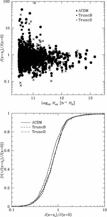
Figure 11. Angular momentum at turnaround. We track the material associated with each halo identified at z=0 and compute the radial extent and angular momentum of this material as a function of redshift in the ΛCDM, TruncB, and TruncD runs. When the material has reached its maximum radial extent, we denote the epoch at which this occurs as turnaround and look at the ratio of the magnitude of angular momentum of the material at this redshift z t, J(z t), with respect to the magnitude of the angular momentum of this material at z = 0. In the upper panel, we show the variation of this ratio with halo mass at z = 0; in the lower panel, we show the cumulative distribution D(<J(z t)/J(z = 0)).
We expect tidal torques arising from gravitational interaction with the surrounding matter distribution to drive the growth of angular momentum at early times (prior to turnaround) and so it should not be particularly sensitive to a small-scale cut-off in the power spectrum. Linear perturbation theory should hold, and the angular momentum of the material should grow in proportion to (1 + z)−3/2 (cf. White Reference White1984). Therefore, we expect the angular momentum at turnaround to be close to its maximum valueFootnote 3 and the frequency distribution of angular momenta should be similar in each of the models we have looked at. Linear perturbation theory no longer provides a good description of angular momentum growth subsequent to turnaround and non-linear processes (i.e. mergers) are believed to become more important drivers of angular momentum evolution during this phase. Therefore, if there are differences between the models, we would expect them to be apparent in the ratio of the ‘peak’ angular momentum at turnaround to the final angular momentum at z = 0.
In the upper panel of Figure 11, we show the distribution of J(z t)/J(z = 0) versus halo mass, while in the lower panel we show the cumulative distribution D(<J(z t)/J(z = 0)) for all haloes with masses in excess of 5 × 10¹⁰ h − 1M⊙ at z = 0. For clarity, we consider only the λCDM (filled circles, solid curves), TruncB (filled squares, dashed curves), and TruncD (crosses, dotted-dashed curves) runs. The upper panel reveals that, on average, the ratio of J(z t)/J(z = 0) does not vary appreciably with mass and that it is slightly less than unity (approximately 0.8). In other words, the magnitude of the total angular momentum of the material at turnaround is on average smaller than at z = 0.
These figures reveal that the small differences that we observe in the spin distributions are also present in the specific angular momentum. The median J(z t)/J(z = 0) differs by ~10% between the ΛCDM model and the TruncD run.
6 SUMMARY AND DISCUSSION
The focus of this paper has been to determine the extent to which suppressing the formation of small-scale structure—low-mass dark matter haloes—affects observationally accessible properties of galaxy-mass dark matter haloes. Using cosmological N-body simulations, we have investigated the spatial clustering of low-mass haloes around galaxy-mass haloes, the rate at which these haloes assemble their mass and at which they experience mergers, and their angular momentum content in a fiducial ΛCDM model and in truncated (ΛWDM-like) models. The main results of our study can be summarised as follows:
Large-scale structure:
Visual inspection of the density distribution reveals that the structure that forms in truncated models is indistinguishable from that in the ΛCDM model on large scales but differs on small scales. Precisely how small this scale is depends on M cut, the mass scale below which low-mass halo formation is suppressed, which we varied between 5×10⁹ h −1M⊙ and 1011 h − 1M⊙. For M cut = 5×10⁹ h −1M⊙, the differences with respect to the ΛCDM model are negligible, but they become significant for M cut = 1011 h − 1M⊙.
Spatial clustering:
These visual differences are apparent in the clustering strength of lower-mass secondary haloes around galaxy-mass primaries. Fixing the primary mass at M vir = 1011 h − 1M⊙, we found that the clustering strength of secondaries around primaries depends strongly on M cut and the minimum secondary mass. If we include secondaries with masses M vir ⩾ 3 × 10⁹ h − 1M⊙, the differences are as great as ~50% when M cut=1011 h − 1M⊙. Unsurprisingly, we found no dependence on M cut if secondaries are restricted to haloes with masses M vir ⩾ 1011 h − 1M⊙.
Mass accretion and merger rates:
The sensitivity of the clustering strength to M cut has immediate consequences for the frequency of minor mergers. The effect is most striking for models with M cut ⩾ 5 × 10¹⁰ h − 1M⊙, when the rate of all mergers with mass ratios in excess of ~6% is suppressed across all redshifts by factors of ~2 to 3 in haloes with virial masses of M vir ≲ 5 × 10¹¹ h − 1M⊙. This effect must be driven by a reduction in the number of minor mergers because the frequency of major mergers does not depend on M cut other than in haloes with masses M vir ~ M cut. Interestingly, we found that the total mass accretion rate does not appear to be sensitive to M cut at all.
Halo angular momentum:
Minor mergers appear to have little influence on the angular momentum content of galaxy-mass haloes.
-
1. We computed the spin parameter λ and found no obvious dependence on M cut but a strong dependence on mass accretion history has—a marked systematic offset is evident between the average spins of haloes with violent mass accretion histories and those with quiescent histories—by a factor of ~2 to 3, independent of M cut. The spin of individual haloes evolves in an almost stochastic fashion over time and on average do not show any obvious evolution with redshift.
-
2. We examined the angular momentum distribution within haloes by constructing specific angular momentum profiles, which quantify the fraction of material within a halo that has specific angular momentum of j or less. We found a weak trend for halo material in truncated models with values of M cut greater than 1010 h − 1M⊙ to have on average smaller values of j by 25% at most, but the r.m.s scatter is large for a given M(<j) in all our models and the differences have a low statistical significance.
-
3. We investigated the angular momentum of the Lagrangian region corresponding to the virialised halo at z = 0 and determined how it evolves with time. We calculated J(z t)/J(z = 0), the ratio of the angular momentum of the material at the turnaround redshift z t to z = 0. Again the differences between the models are small, at most 10%.
These results indicate that small-scale structure has little impact on the angular momentum content of galaxy-mass haloes, in broad agreement with those of Wang and White (Reference Wang and White2009), who studied halo formation in hot dark matter models, and Bullock et al. (Reference Bullock, Kravtsov and Colín2002) and Chen and Jing (Reference Chen and Jing2002), who looked at WDM models.
These results show that there are differences in the spatial clustering and merger rates of low-mass haloes between our fiducial ΛCDM model and the truncated models—but that they are evident only in the most extreme truncated models, with M cut in excess of 1010 h −1M⊙. As we noted in the introduction, this is inconsistent with astrophysical constraints on the putative WDM particle mass. Therefore, measuring the effect on spatial clustering or the merger rate is likely to be observationally difficult for realistic values of M cut, equivalent to our TruncA runs, and so isolating the effect of this small-scale structure would appear to be remarkably difficult to detect, at least in the present day Universe.
However, there are important caveats. The effect may not be so subtle in the high redshift Universe, during the earliest epoch of galaxy formation, and so we might expect marked differences in the abundances of low-mass satellites between our fiducial ΛCDM model and WDM or truncated models. This may have observable consequences for the ages and metallicities of the oldest stars in galaxies (e.g. Frebel Reference Frebel2005), the abundance of metal poor globular clusters, and the assembly of galaxy bulges and stellar haloes. In addition, there is no compelling reason to expect that the efficiency of galaxy formation will differ between a ΛCDM model and a WDM or truncated model, and so it may be the case that galaxy formation in a WDM(-like) model is easier to reconcile with the observed galaxy population than galaxy formation in the fiducial ΛCDM model (see also Menci et al. Reference Menci, Fiore and Lamastra2012; Benson et al. Reference Benson2013). We shall return to these ideas in forthcoming work.
ACKNOWLEDGEMENTS
CP thanks the anonymous referee for their thoughtful report. This work was supported by ARC DP130100117 and by computational resources on the EPIC supercomputer at iVEC through the National Computational Merit Allocation Scheme. The research presented in this paper was undertaken as part of the Survey Simulation Pipeline (SSimPL; http://ssimpl-universe.tk/).


