


1 INTRODUCTION
When identifying strategies for the development of instrumentation for astronomy, it is clear that some of the most important themes of current research such as ‘What are the conditions for planet formation and the emergence of life?’ and ‘How did the Universe originate and what is it made of?’ can only be fully answered with observations in the mid- to far-infrared part of the spectrum. This domain is virtually inaccessible from the ground because the Earth’s atmosphere is opaque to infrared radiation, and therefore sensitive space-based observations are required which provides the impetus for the SPICA mission concept described in this paper.
Over the past three decades, we have come to understand that at least half of the energy ever emitted by stars in galaxies is to be observed in the infrared (see e.g. Dole et al. Reference Dole2006). Observations at IR wavelengths are optimal for the study of galactic evolution in which peak activity occurs at redshifts of z ~1–4, when the Universe was roughly 2–3-Gyr old—as was concluded primarily through deep and wide-field observations with previous infrared space observatories: IRAS (Neugebauer et al. Reference Neugebauer1984), ISO (Kessler et al. Reference Kessler1996), Spitzer (Werner et al. Reference Werner2004), AKARI (Murakami et al. Reference Murakami2007), Herschel (Pilbratt et al. Reference Pilbratt2010), and WISE (Wright et al. Reference Wright2010). In addition, many of the basic processes of star formation and evolution, from pre-stellar cores to the clearing of gaseous protoplanetary discs, and the presence of dust excess around main-sequence stars, were discovered by these pioneering missions. Notwithstanding the success of these missions, these observatories either had small cold telescopes, or large, warm mirrors, ultimately limiting their ability to probe the physics of the faintest and most distant, obscured sources that dominate the mid- and far-infrared emission in our Universe.
1.1. The power of infrared diagnostics
The mid- to far-IR spectral range hosts a suite of ionic, atomic, molecular, and dust features covering a wide range of excitation, density, and metallicity, directly tracing the physical conditions both in the nuclei of galaxies and in the regions where stars and planets form (see Figures 1–3). Ionic fine structure lines (e.g. [Ne ii], [S iii], and [O iii]) probe H ii regions around hot young stars, providing a measure of the star-formation rate, stellar type, and the density of the gas. Lines from highly ionised species (e.g. [O iv] and [Ne v]) trace the presence of energetic photons emitted from AGN, providing direct measures of the accretion rate. Photo-dissociation regions (PDR), the transition between young stars, and their parent molecular clouds, can be studied via the strong [C ii] and [O i] lines and the emission from small dust grains and PAHs. The major coolants of the diffuse warm gas (e.g. [N ii]) in galaxies also occur in the far-infrared giving us a complete picture of the ISM.
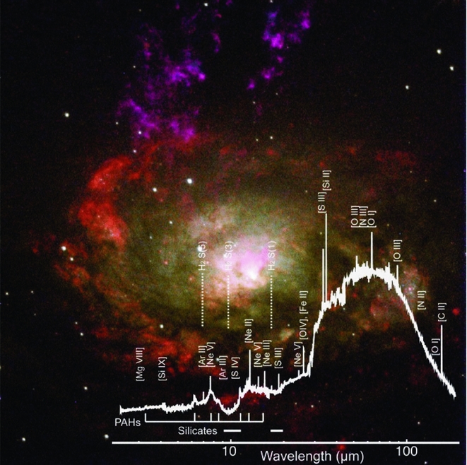
Figure 1. ISO 2–200 μm spectrum of the Circinus galaxy showing the bright IR peak and the wealth of spectral features including fine structure ionic lines, molecular lines, and PAH features (Moorwood Reference Moorwood, Cox and Kessler1999). The background shows a Hubble Space Telescope image of the galaxy (Wilson et al. Reference Wilson, Shopbell, Simpson, Storchi-Bergmann, Barbosa and Ward2000) offering exquisite detail but capturing only a small fraction of the total energy produced by the galaxy—most of which emerges in the mid- and far-IR.

Figure 2. Model SED for a protoplanetary disc, illustrating that the bulk of the planet-forming reservoir is best studied at mid- to far-IR wavelengths, but requires high sensitivity for the detection of gas lines and dust/ice features.
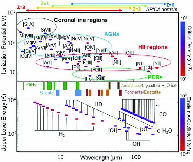
Figure 3. Upper panel: Ionisation potential versus wavelength for key infrared ionic fine-structure lines (Spinoglio & Malkan Reference Spinoglio and Malkan1992). Lower panel: Upper energy level of molecular transition and spectral features from PAHs, water ice bands, and other species versus wavelength. The SPICA domain is indicated above for several different redshifts.
The rest-frame infrared furthermore is home to pure rotational H2, HD, and OH lines (including their ground state lines) and mid- to high-J CO and H2O lines, most notably the H2O ground state line at 179 μm. Finally, the strong PAH emission features (carrying 1–10% of the total IR emission in star-forming galaxies) with their unique spectral signature, can be used to determine redshifts of galaxies too dust-obscured to be detected at shorter wavelengths. The infrared also hosts numerous unique dust features from minerals such as olivine, calcite, and dolomite that probe evolution from pristine to processed dust (e.g. aqueous alteration), as well as CO2 ice and molecules like C2H2 and fullerenes. A table listing these various spectral tracers can be found in van der Tak et al. (Reference van der Tak2017).
Taking advantage of progress in detector performance and cryogenic cooling technologies, we now stand on the threshold of unprecedented advances in our ability to study the hidden, dusty Universe. An observatory like SPICA as presented in this paper, with a large, cold telescope complemented by an instrument suite that exploits the sensitivity attainable with the low thermal background, can in the mid-/far-infrared achieve a gain of over two orders of magnitude in spectroscopic sensitivity as compared to Herschel, Spitzer, and SOFIA (Becklin, Young, & Savage Reference Becklin, Young and Savage2016, see also Figure 4). In addition, such a mission will provide access to wavelengths well beyond those accessible with the James Webb Space Telescope (JWST, Gardner et al. Reference Gardner2006) and the new generation of extremely large telescopes (Tamai et al. Reference Tamai, Cirasuolo, González, Koehler and Tuti2016; McCarthy et al. Reference McCarthy2016). Sitting squarely between JWST and ALMA (Wootten & Thompson Reference Wootten and Thompson2009), SPICA will enable the discovery and detailed study of the coldest bodies in our Solar System, emerging planetary systems in the Galaxy, and the earliest star-forming galaxies and growing super-massive black holes—a gigantic leap in capabilities for unveiling the ‘hidden Universe’. With its large cryogenic infrared space telescope, SPICA will allow astronomers to peer into the dust-enshrouded phases of galactic, stellar and planetary formation and evolution, revealing the physical, dynamical, and chemical state of the gas and dust, and providing answers to a range of fundamental astronomical questions:
• What are the roles of star formation, accretion onto and feedback from central black holes, and supernova explosions in shaping galaxy evolution over cosmic time?
• How are metals and dust produced and destroyed in galaxies? How does the matter cycle within galaxies and between galactic discs, halos, and intergalactic medium?
• How did primordial gas clouds collapse into the first galaxies and black holes?
• What is the role of magnetic fields at the onset of star formation in the Milky Way?
• When and how does gas evolve from primordial discs into emerging planetary systems?
• How do ices and minerals evolve in the planet formation era, as seed for Solar Systems, acting as the seeds for planet formation?
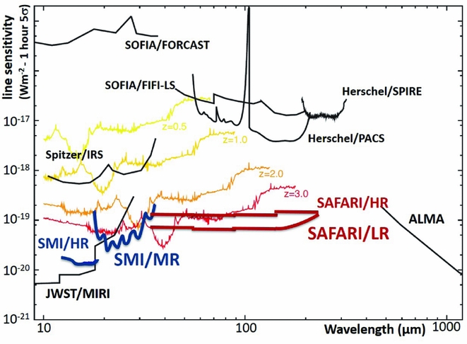
Figure 4. Projected spectroscopic sensitivity of the SPICA instruments as compared to other infrared facilities (at the SAFARI/LR resolution of ~300). The SAFARI sensitivity assumes a detector NEP of 2 × 10⁻¹⁹ W √Hz−1. The infrared spectrum of the Circinus galaxy, scaled to L = 1012 L⊙, for redshifts 0.5 to 3, and smoothed to the SAFARI/LR resolution, is superimposed.
These questions, their background science, and how SPICA would help resolve them, are discussed in much more detail in a dedicated series of papers (Spinoglio et al. Reference Spinoglio2017; Fernández-Ontiveros et al. Reference Fernández-Ontiveros2017; González-Alfonso et al. Reference González-Alfonso2017; Gruppioni et al. Reference Gruppioni2017; Kaneda et al. Reference Kaneda2017; E. Egami et al., in preparation; van der Tak et al. Reference van der Tak2017; P. André, in preparation; Trapman et al. Reference Trapman, Miotello, Kama, van Dishoeck and Bruderer2017; Notsu et al. Reference Notsu, Nomura, Ishimoto, Walsh, Honda, Hirota and Millar2017, Reference Notsu, Nomura, Ishimoto, Walsh, Honda, Hirota and Millar2016; I. Kamp Reference Kamp, Scheepstra, Min, Klarmann and Riviere-Marichalar2018).
1.2. A cryogenic infrared space telescope
Early mission concepts for a cryogenic infrared space telescope, initially proposed by the Japanese space agency JAXA, have been described extensively elsewhere (Nakagawa et al. Reference Nakagawa, Bely and Breckinridge1998; Swinyard et al. Reference Swinyard2009; Nakagawa et al. Reference Nakagawa, Shibai, Onaka, Matsuhara, Kaneda, Kawakatsu and Roelfsema2014). Over time the mission concept has evolved significantly, SPICA is now envisaged as a joint European–Japanese project to be implemented for launch and operations at the end of the next decade. As an ESA mission, the project would go to through the standard ESA phasing and milestones, starting with the detailed Phase A study in 2019/2020 and mission selection in early 2021. A joint ESA–JAXA study was already conducted to assess the technical and programmatic feasibility of possible mission configurations (Linder et al. Reference Linder, Falkner, Puig, Renk, Doyle, Timm, Symonds and Walker2014), the satellite configuration has since been further optimised.
In the currently foreseen architecture, building on heritage from the ESA Planck mission (Planck Collaboration et al. 2011), the optical axis of the 2.5-m diameter cold telescope is perpendicular to the axis of the spacecraft and ‘V-groove’ radiators, mounted between the telescope assembly and the satellite service module (SVM), provide very efficient passive cooling. The solar cells to provide power are mounted on the bottom side of the SVM, which is always orientated towards the Sun. In parallel with this optimisation of the mission concept, the science payload has also been revisited and upgraded. The resulting mission concept as considered in this paper will provide extremely sensitive—of order 5× 10⁻²⁰ W m−2 (5σ/1 h)—spectroscopic capabilities from 17 through 230 μm at resolutions ranging from R = 50 to 11 000. A high resolution R ~28.000 capability is provided for the 12–18 μm wavelength range. Efficient broadband photometric mapping can be carried out in the 30–37 μm domain, as can spectroscopic imaging for small fields in the 35–230 μm range. In addition, a polarimetric imaging capability is provided in three bands at 100, 200, and 350 μm. The spectroscopic sensitivity (Figure 4) of the instrument suite will typically provide two orders of magnitude improvement over what has been attained to date, corresponding to a truly enormous increase in observing speed. Such an exceptional leap in performance is bound to produce many scientific advances. Some of these are predictable today and form the core science case for a SPICA concept and will drive its design. However, many additional advances are impossible to predict, and the discovery space is undoubtedly large in such a mission.
2 THE SPICA SATELLITE CONCEPT
The SPICA mission concept utilises a 2.5-m class Ritchey–Chrétien telescope, cooled to below 8 K. The telescope is mounted on the SVM with its axis perpendicular to the spacecraft axis. The practical telescope size is primarily limited by the launcher capabilities—fairing diameter and mass capability. The telescope and instrument suite, which are never exposed to direct sunlight, will be cooled using mechanical coolers in combination with V-groove radiators. Solar panels to provide electrical power are mounted on the bottom of the SVM, which is directed towards the Sun. The nominal mission lifetime is 3 yr, with a goal of 5 yr, but as cooling is provided by mechanical coolers, the operational lifetime in practice would not be limited by liquid cyrogen consumables but only by the available propellant and the durability of mechanisms and on-board electronics.
The overall configuration of the spacecraft concept is shown in Figure 5, with the SVM housing the general spacecraft support functions below, and on the top the payload module (PLM) with the Science Instrument Assembly (SIA), and the Cryogenic Assembly (CRYO) housing the passive and active cooling system for the SIA. Figure 6 shows the telescope configuration on the left and on the right a tentative focal plane aperture assignment for the instruments and the two Focal Plane Attitude Sensors (FAS) (part of the overall spacecraft pointing system). The main parameters of the satellite are summarised in Table 1.
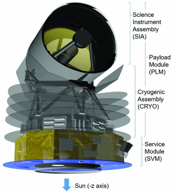
Figure 5. The SPICA spacecraft configuration. The scientific instruments are mounted on the optical bench on the rear of the telescope (see also Figure 6).
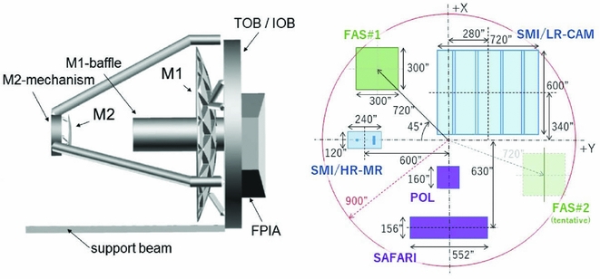
Figure 6. Left: Configuration of the SPICA telescope assembly. The scientific instruments are mounted in Focal Plane Instrument Assembly (FPIA), on the optical bench on the rear of the telescope. Right: The SPICA instrument focal plane layout.
Table 1. Main SPICA mission parameters.

The SPICA telescope derives directly from the Herschel mission, in design as well as implementation. The system optical design is based primarily on the ESA CDF study (Linder et al. Reference Linder, Falkner, Puig, Renk, Doyle, Timm, Symonds and Walker2014) with further follow-up work at JAXA. The overall layout for the telescope optics is shown in Figure 6. The telescope primary and secondary mirrors and the secondary supports will be made of silicon carbide (SiC), exploiting the heritage of the Herschel, AKARI, and Gaia missions in terms of structure and technology and materials. The entire telescope assembly will be cooled down to <8 K. Because of the extremely low power radiant levels at the detectors, stray-light rejection will be an important consideration in the detailed design of the telescope baffle and the instrument optics. Estimates for the wavefront error budget indicate that the secondary assembly will require a three-axis (focusing, tip, and tilt) correction mechanism, which can be driven by actuators similar to those used on the Gaia spacecraft (Gaia Collaboration et al. 2016).
2.1. The cryogenic assembly
The PLM is connected by trusses to the CRYO, consisting of the Cooler Module and the Thermal Insulation and Radiative Cooling System. The Cooler Module houses the mechanical cryocooler units with their electronics, and the warm electronics modules of the science instruments. The CRYO is designed with the primary goal to cool the telescope assembly (STA) to below 8 K, and to provide cold temperature stages for the instruments at 4.8 and 1.8 K. The system is designed to reach a steady state for those temperatures within 180 d after launch. The SPICA cooling system combines radiative cooling with V-Groove shields similar to the Planck design (Planck Collaboration et al. 2011) with mechanical cryocoolers (Sugita et al. Reference Sugita2010; Shinozaki et al. Reference Shinozaki2014). In addition, a telescope shield, which is actively cooled down to 25 K, is placed between the V-Grooves and the telescope baffle (Ogawa et al. Reference Ogawa2016).
The spacecraft will keep its attitude always with the −Z axis directed towards the Sun (see Figure 5), such that only the solar panel on the bottom of the SVM is illuminated and the SIA is never exposed to direct solar radiation. Only the actively cooled telescope shield and deep space are within the SIA field-of-view.
The proposed CRYO is shown in Figure 7. A trapezoidal platform made of carbon fibre reinforced plastic (CFRP), with six CFRP bipods, forms a stable, light-weight structure acting as a mounting platform for the cold telescope. The struts of the telescope optical bench support structure are made of low-thermal-conductivity CFRP to reduce the conducted heat load from the warm SVM. The bipods and telescope optical bench support need to be substantial enough to satisfy the spacecraft stiffness requirements and withstand the launch loads. However, they will also be the main conductive heat path from SVM to SIA, requiring very low thermal conductance. Therefore, an on-orbit truss separation mechanism (Mizutani et al. Reference Mizutani, Yamawaki, Komatsu, Goto, Takeuchi, Shinozaki, Matsuhara and Nakagawa2015) will be used to de-couple strong supports after launch, when high mechanical strength will no longer be necessary, leaving only the low-conductance supports. Six interface points between bipods and the platform (indicated with red circles in Figure 7) will be separated using a CFRP octagonal spring mechanism leaving the SVM and SIA connected only by the low-thermal-conductance elements. Each of the three V-groove shields, attached to the bipods, is constructed of sandwich panels with aluminium face sheets and an aluminium honeycomb core. The telescope shield is an aluminium shell or full aluminium sandwich panel, supported by the bipods.
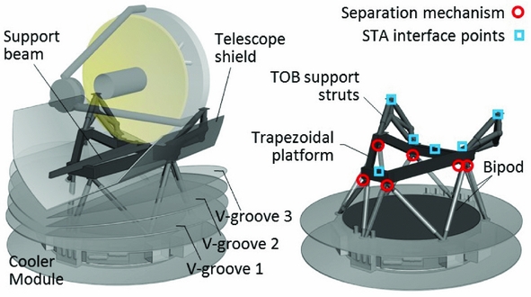
Figure 7. External view of the SPICA cryogenic support structure with bipods, V-groove shields, and trapezoidal mounting platform for the telescope assembly.
The SPICA cooling chain concept (Shinozaki et al. Reference Shinozaki2016) is shown in Figure 8. The system has two chains for the SIA, one to provide a 4.8-K level and the other to provide a 1.8-K level. Both chains use two types of Joule–Thomson coolers (4 K-JT and 1 K-JT) in combination with three double-stage Stirling (2ST) pre-coolers. The telescope shield is cooled to about 25 K by two dedicated 2ST coolers, and three V-groove shields are used to reduce the heat load to the telescope shield. Redundant chains are provided as safeguard against failures in any one of the coolers.
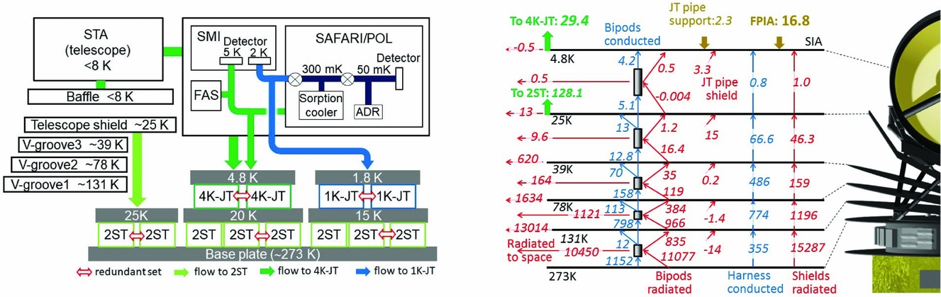
Figure 8. The SPICA cryogenic system. Left: The cooling chain concept. 4 K-JT and 1 K-JT coolers are used to cool the STA and instrument focal plane units, and used as pre-coolers for the SAFARI and POL sub-K coolers (sorption cooler and adiabatic demagnetisation refrigerator—ADR). The redundant chains provide a safeguard against failures in any one of the coolers. Right: A heat flow diagram (values in mW). With the maximum heat load (16.8 mW) from the instruments, the estimated heat flow to the 4 K-JT is 29.4 mW, well below the 40 mW end-of-life cooling capability of the 4 K-JT system with one failed cooler.
One of the challenges for the SPICA project will be the validation of the SPICA cryogenic system, as its performance is of prime importance for the success of the mission. For this validation, an extensive ground test programme will need to be executed in which the full payload—i.e. the integrated telescope and instrument assemblies—as well as relevant test sources are operated under flight-like conditions.
2.2. Service module (SVM)
The SPICA SVM (see Figure 9), housing all spacecraft support functions, is considered fairly standard and can be derived directly from, e.g. the Herschel and Planck missions. It will be a combination of a thrust cone as load path between PLM and the launcher, and shear panels. The top and bottom platforms and the side panels accommodate spacecraft equipment. The solar panels are mounted on the lower platform and always face the Sun. To maintain the units inside the SVM at their nominal operating temperature, the bottom and top platforms are insulated from the rest of SVM by means of Multi-Layer Insulation (MLI) and thermal stand-offs. The top surface facing the PLM is also covered with MLI.
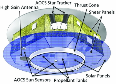
Figure 9. The SPICA service module (SVM).
The baseline data handling system architecture comprises of an on-board computer, remote terminal units, and solid state mass memory. The platform generates about 15-kbps housekeeping data rate, and the science instruments generate data at an average rate of 3 Mbps with around 15 kbps of instrument housekeeping. The mass memory will need to be able to store up to 72 h of spacecraft data (roughly 100 GB). To a large extent, the SVM sub-systems, also including the Command and Data Handling subsystem, are based on highly recurrent designs and little need for technology developments is expected. Nominal telemetry and telecommand operation as well as scientific telemetry downlink use X-band frequencies. Low gain antennas are positioned such that continuous coverage is achievable for low data rate command and housekeeping. A high gain antenna is mounted on the bottom panel of the spacecraft which in nominal attitude points towards the Earth. The proposed architecture will have active redundancy for the uplink and passive redundancy for the high data rate downlink.
The Attitude and Orbit Control Subsystem (AOCS) will use a three-axis stabilised system based on a star-tracker and gyro estimation filter for coarse pointing modes, with a design derived directly from the Herschel AOCS architecture. In addition, a FAS is likely to be needed to fulfil the more stringent requirements in some of the science fine pointing modes. Two (redundant) FAS cold units, housing the camera optics and 1 K × 1 K near-IR detectors, will be mounted on the SIA, with warm signal processing electronics in the SVM. The FAS has a 5 arcmin × 5 arcmin FoV (see Figure 5), which can track at least five stars at any one time. For science observations, the AOCS will be required to achieve a pointing accuracy of order 0.5 − 1 arcsec, depending on the details of the observing mode. The absolute pointing error budget contributions come from three different main sources: the structure misalignment between the instruments and FAS, the FAS constant bias, and controller performance including actuator disturbance noise. The relative pointing error is mainly due to three contributors: attitude relative pointing estimates (FAS + gyros), short-term controller performance including actuator noise, and μ-vibration sources (reaction wheels and cryocoolers). The a-posteriori absolute pointing knowledge error budget is linked to the attitude estimate error achievable on-board with possible corrections obtained by post-processing on ground.
3 NOMINAL INSTRUMENT COMPLEMENT
3.1. A far-infrared spectrometer
With galaxy evolution over cosmic time as a main science driver, the SPICA far-infrared spectrometer SAFARI is optimised primarily to achieve the best possible sensitivity, within the bounds of the available resources (thermal, number of detectors, power, and mass), at a moderate resolution of R ~300, with instantaneous coverage over the full 34 to 230 μm range. A secondary driver is the requirement to study line profiles at higher spectral resolution, e.g. to discern the in-fall and outflow of matter from active galactic nuclei and star-forming galaxies. This leads to the implementation of an additional high resolution mode using a Martin–Puplett interferometer (Martin & Puplett Reference Martin and Puplett1970). With this design, the sensitivity of the R ~300 SAFARI/LR mode will be about 5 × 10⁻²⁰ W m−2 (5σ, 1 h) assuming a TES (Transition Edge Sensor) detector NEP (Noise Equivalent Power) of 2 × 10⁻¹⁹ W √Hz−1. With such high sensitivity, astronomers will be able to characterise, over the full spectral band, average-luminosity galaxies (~L *) out to redshifts of at least 3. It should be noted that in this design concept, with essentially zero background emission from the telescope and instruments, further advances in detector sensitivity translate directly to better overall instrument performance.
A functional block diagram for the SAFARI spectrometer system is shown in Figure 10. It illustrates the division of the system into two major elements on the spacecraft; the top of the diagram shows the cold focal plane unit (FPU) mounted on the optical bench (at 4.8 K) and the lower part the warm electronics mounted on the CRYO assembly (see also Figure 5). The signal from the telescope is fed into the instrument by a pick-off mirror in the common instrument focal plane (see Figure 6). The baseline SAFARI design uses a 2D beam steering mirror (BSM) in an Offner relay to send the incoming signal to the dispersion and detection optics. The BSM can be used to select either the sky or an internal calibration signal, and convey this to either the nominal R ~300 (SAFARI/LR) resolution optics chain or to the R ~2 000–11 000 resolution SAFARI/HR optics chain. The full 34–230 μm wavelength range is covered by four separate bands, each with its own grating and detector array. The signal is conditioned and split over these four wavelength bands, using band defining filters and dichroics, for input into the Grating Modules (GM, see Section 5.1.1) which house the grating optics and the band detector modules. The spectrometer specifications and capabilities are listed in Table 2.
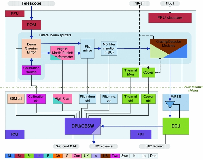
Figure 10. The functional block diagram for SAFARI. The top part represents the focal plane unit mounted on the 4.8-K instrument optical bench. The bottom part shows the warm electronics, mounted on the CRYO assembly.
Table 2. SAFARI performance summary.
High R—high resolving power mode; R ~ 11000 at 34 μm to R ~ 1500 at 230 μm Nominal R—nominal resolving power; R ~ 300 5σ confusion—5σ confusion limit.
The operation of SAFARI will be controlled by an Instrument Control Unit (ICU). The ICU will receive instrument commands from the spacecraft, interpret and validate them, and subsequently operate all the different SAFARI units in accordance with these commands. In parallel, the ICU will collect housekeeping data from the various subsystems and use these to monitor the instrument health and observation progress. The ICU will also collect the science data pre-conditioned in the Warm Front End Electronics (WFEE) and acquired by the Detector Control Unit (DCU), and package these data along with the housekeeping information for transmission to the spacecraft mass memory from where it will be subsequently downloaded to the ground.
3.1.1. The SAFARI detector grating modules
The low-resolution dispersion is effected through diffraction gratings illuminating the detector arrays. By so doing the photon noise is reduced to that arising from the narrowband viewed by each detector, allowing the high sensitivity offered by the state-of-the-art TES detectors to be fully utilised. A generic GM design is used for the four bands, with the infrared beam entering through an input slit and propagating via a collimator and a flat mirror to a high incidence grating. A mirror refocuses the dispersed signal onto the detector arrays. The practical size limit for the GM dictates the use of a high incidence grating, which allows for a more compact optics layout. As a result, the GM is efficient for only a single polarisation.
All elements in the GM are within a light-tight 1.8-K enclosure. Equally important, this enclosure provides shielding for the sensitive TES detectors and SQUID readouts against electromagnetic interference (EMI). The very long wavelength GM is shown in the right panel of Figure 11 as an example of the GM design.
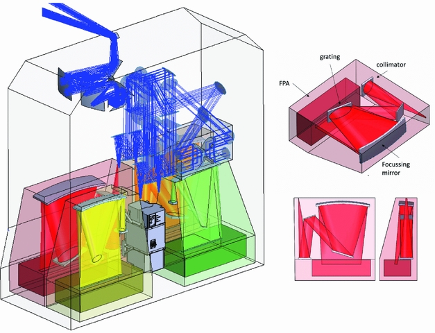
Figure 11. Left: The SAFARI focal plane unit (FPU) as it is mounted against the back of the telescope. The beam from the telescope secondary comes from the top left and is sent into the instrument via the pick-off mirror on the top of the instrument box. From there, it goes into the Offner relay optics and on to the Beam and Mode Distribution Optics. On the right, the Martin–Puplett signal path and its moving mirror stage can be seen. Three of the four grating modules (red: VLW, yellow: MW, and green: SW) are visible on the bottom, the LW band GM (orange) is at the back. Between the MW and SW grating modules, the cooler unit (grey) is visible. Right: Schematic views of the SAFARI Very Long Wavelength band Grating Module. The location of the detector module as shown in Figure 12 is indicated by the rectangular box denoted as FPA.
SAFARI employs the latest generation of ultra-sensitive TES to detect the incoming photons (Khosropanah et al. Reference Khosropanah2016; Audley et al. Reference Audley, de Lange, Gao, Khosropanah, Hijmering and Ridder2016; Suzuki et al. Reference Suzuki2016; Goldie et al. Reference Goldie2012; Beyer et al. Reference Beyer2012). TES bolometers fabricated at SRON (Ridder et al. Reference Ridder, Khosropanah, Hijmering, Suzuki, Bruijn, Hoevers, Gao and Zuiddam2016) have already demonstrated the required NEP (Khosropanah et al. Reference Khosropanah2016), as well as the required optical efficiency (Audley et al. Reference Audley, de Lange, Gao, Khosropanah, Hijmering and Ridder2016). To achieve their performance, the detectors, their readout, and the first-stage amplifiers must be operated at 50-mK, which requires that both the sensors and the cold electronics be cooled and thermally isolated from the 1.8-K environment of the GM. This is achieved in two steps, with the TES and cold readout electronics in a 50-mK structure suspended, using Kevlar wires, from a 300-mK enclosure (the grey box in Figure 12). The 300-mK enclosure, providing additional radiation shielding, is again suspended using Kevlar from the 1.8-K GM enclosure. The signal is coupled to the TES using 1.5-Fλ horns. There are three parallel linear TES arrays in the focal plane assembly (FPA), thus constituting at each wavelength three separate spatial pixels, to provide background reference measurements for point source observations and redundancy against individual failures in TES sub-arrays. The three spatial pixels also provide a limited imaging capability.
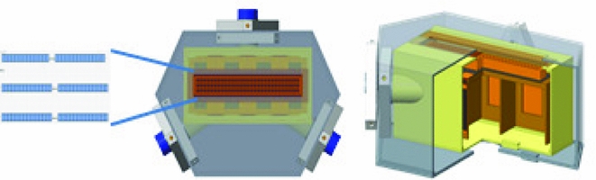
Figure 12. A generic 300-mK SAFARI detector module. Left: Schematic showing three lines of 1.5-Fλ size detectors, separated by 4-Fλ. Centre: Front view with horns in front of the TESs. The yellow box houses the 50-mK detector elements. The blue studs indicate the Kevlar suspension connection points, from 50 mK to 300 mK, to the 1.8-K structure. Right: cut-out view showing the cold readout AC biasing electronics, SQUIDs, and LC filters.
With some 3 500 individual TES detectors in SAFARI system, a detector readout multiplexing scheme is essential to limit the amount of wiring between the FPU and the warm electronics (WFEE, DCU, and ICU) on the spacecraft SVM. A Frequency Domain Multiplexing (FDM) readout scheme will be employed in which each of the detectors in one multiplex channel is AC biased at a different frequency. The combined signals of the detectors in one channel are de-multiplexed and detected in the backend DCU. Multiplexing 160 detectors per channel, the designed flight configuration, has already been demonstrated in a laboratory setup at SRON (Hijmering et al. Reference Hijmering, den Hartog, Ridder, van der Linden, van der Kuur, Gao and Jackson2016).
To cool the TES detectors to their 50 mK operating temperature, a dedicated hybrid ADR/Helium sorption cooler is used. The cooler design builds on heritage from the Herschel and Planck missions. A full design has already been carried out for SAFARI, leading to the construction of an Engineering Model. Tests with the Engineering Model show that the unit will be able to provide the required level of cooling with a ~80% duty cycle (Duband, Duval, & Luchier Reference Duband, Duval and Luchier2014). The same cooler design will be used both for SAFARI and POL (see Section 5.3).
3.1.2. The high-resolution mode optics—The Martin–Puplett interferometer
In the high-resolution SAFARI/HR mode, the infrared beam is passed through a Martin–Puplett interferometer [Figure 13, see also Martin & Puplett (Reference Martin and Puplett1970)] which imposes a modulation on all wavelengths entering SAFARI. The resulting interference that occurs between the two beams of the interferometer is then distributed to the four GM (Figure 11) and post-dispersed by the corresponding grating onto the detectors.
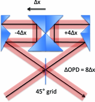
Figure 13. A Martin–Puplett interferometer: A linearly polarised input signal is divided over two arms of the interferometer using a 45° grid. In both arms, the beam goes via a flat mirror to a moving and a fixed rooftop and back, thus rotating the polarisation three times by 90°. This 270° rotated signal from the left arm is transmitted through the grid, while from the right arm it is reflected, allowing the recombined beams to interfere. By moving the central rooftop mirrors over a distance Δx, an optical path length difference of 8Δx is created between the two arms. The interference pattern, encoded in the polarisation of the output signal, can be recorded by the grating module, due to its inherently linear polarisation.
When the interferometer is scanned over its full optical displacement, each of the detectors will measure a high-resolution interferogram convolved with the grating response function for that particular detector. Upon Fourier transformation, an individual interferogram produces a small bandwidth, high-resolution spectrum. By combining the spectra from individual detectors, a full spectrum at high resolution is obtained. In the current design, a mechanical displacement of about 3 cm is envisaged, leading, with a folding factor of 8, to a maximum optical displacement of 25 cm. A short section of the mechanism stroke must be devoted to a short double-sided optical path difference measurement to enable phase correction of the interferogram through accurate identification of the zero path difference position. The available optical path difference yields spectra with a resolving power ranging from R ~1 500 at 230 μm to as high as R ~11 000 at the shortest wavelength of 34 μm.
3.1.3. Observing with SAFARI
SAFARI will have a number of observing modes. Intrinsic to the design is instantaneous access to the full 34–230 μm wavelength domain. Thus, in any mode, point source or mapping, low or high resolution, a full spectrum will be obtained. The basic modes will be optimised for maximum efficiency for point source spectroscopy. In the R ~300 grating mode, point source spectra will be obtained using the BSM to chop between the source and a background off-source position, with the difference between the two giving a direct measure of the source flux. By chopping over a distance corresponding to the offset between the three pixel rows in the detector units, there will always be one pixel on-source and two off-source, so that there will be no time penalty for the background chopping. In the SAFARI/HR mode, chopping is not utilised because the scanning of the Martin–Puplett stage provides the modulation needed to correct for instrument drifts. Mapping modes are implemented using the BSM, providing a way to efficiently and flexibly cover small areas (<2 arcmin) without requiring spacecraft repointing. For larger maps, on-the-fly mapping modes will be implemented in which the spacecraft slowly ‘paints the sky’, while the spectrometer continuously records data.
3.2. The mid-infrared instrument SMI
The SMI mid-IR spectrometer/camera is designed to cover the wavelength range from 12 to 36 μm with both imaging and spectroscopic capabilities. The instrument employs four separate channels: the low-resolution spectroscopy function SMI/LR, the broadband imaging function SMI/CAM, the mid-resolution spectroscopy function SMI/MR, and the high-resolution spectroscopy function SMI/HR. The prime science drivers for these functions are high-speed PAH spectral mapping of galaxies at z > 0.5 with SMI/LR, wide-area surveys of obscured AGNs and starburst galaxies at z > 3–5 with SMI/CAM, and velocity-resolved spectroscopy of gases in protoplanetary discs with SMI/HR. Complementary to these specific functions, SMI/MR provides more versatile spectroscopic functions, bridging the gap between JWST/MIRI (Rieke et al. Reference Rieke, Wright, Glasse and Ressler2010) and SAFARI.
A functional block diagram for the SMI is shown in Figure 14 with two main optics chains, one for SMI/LR–CAM and one for the SMI/MR–HR combination, each with their appropriate fore- and aft-optics. The only moving parts within SMI are the shutter in the SMI/LR–CAM chain and the BSM in the SMI/MR–HR chains. Table 3 lists the SMI specifications.
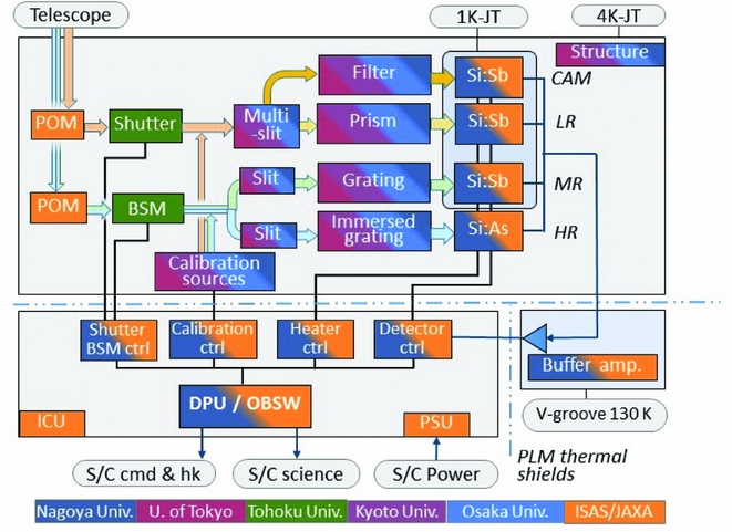
Figure 14. The SMI functional block diagram. The top half of the diagram represents the cold focal plane unit with its two sections. The top CAM/LR arm with the multislit/prism combination provides the combined fast wide field imaging and R ~150 spectroscopy mode. The bottom arm with a beam steering mirror (BSM) forwarding the signal to a slit/grating for the R ~2 000 MR mode, or to a slit/immersed grating for the R ~28 000 mode. The detector readout signals are sent through buffer amplifiers at the 130 K level to the instrument Data Processing Unit (DPU) where the data are packaged for downlink.
Table 3. SMI performance parameters.
SMI/LR is a multi-slit prism spectrometer with a wide field-of-view using four 10 arcmin long slits to execute low-resolution (R = 50–120) spectroscopic surveys with continuous coverage over the 17–36 μm wavelength domain. In SMI/LR, a 10 arcmin × 12 arcmin slit viewer camera is implemented to accurately determine the positions of the slits on the sky for pointing reconstruction in creating spectral maps. This function provides an effective broadband imager centred at 34 μm—SMI/CAM. Both the spectrometer and the camera employ Si:Sb 1 K × 1 K detector arrays. In the SMI/LR spectral mapping mode, the multi-slit spectrometer and the camera are operated simultaneously, yielding both multi-object spectra from 17 to 36 μm as well as R = 5 deep images at 34 μm. The SMI/MR grating spectrometer covers the 18–36 μm wavelength range with a resolving power of R = 1300–2300. The system employs a combination of an echelle grating and a cross-disperser. Like SMI/LR–CAM also this unit uses a 1 K×1 K Si:Sb array for detection of the dispersed infrared beam. SMI/HR is a high-resolution spectrometer covering the 12–18 μm wavelength range at R ~28 000. This high resolution is achieved through the combination of an immersed grating and a cross-disperser using a 4-arcsec long slit. For this spectrometer, a 1 K×1 K Si:As array is used as the detector.
3.2.1. Optical design of SMI
The optical layout of SMI is shown in Figure 15. The design for SMI/LR–CAM and SMI/MR is based on reflective optics with aluminium free-form mirrors, while for the SMI/HR mainly refractive optics with lenses made of KRS-5, KBr, or CdTe are used. The fore-optics, optimised to remove the aberrations due to curvature and astigmatism in the incident beam, relay the telescope beam into the system. For SMI/LR–CAM (Figure 15 right), a multi-slit plate with four slits, of 10-arcmin length and 3.7-arcsec width, with a reflective surface is placed in the focal plane of the rear-optics entrance. The beam passing through the slits is directed to the spectrometer optics, while the beam reflected by the slit-plate is forwarded to the viewer channel optics. A KRS-5 prism in the pupil of the rear-optics of the spectrometer disperses the beam. In front of the slit-viewer detector, a 34 μm R ~ 5 bandpass filter defines the bandpass for broadband photometry. A wide field-of-view is realised with compact reflective optics using the sixth-order polynomial free-form mirrors. Diffraction-limited imaging performance is achieved (i.e. Strehl ratio >0.8) for a 10 arcmin × 12 arcmin field-of-view at 17 μm for the spectrometer and at 30 μm for the viewer. The spectral resolution varies with wavelength from R ~50 at 17 μm to ~120 at 36 μm with slight (<10%) differences between slits and positions within a slit (see Figure 15 right, top panel).
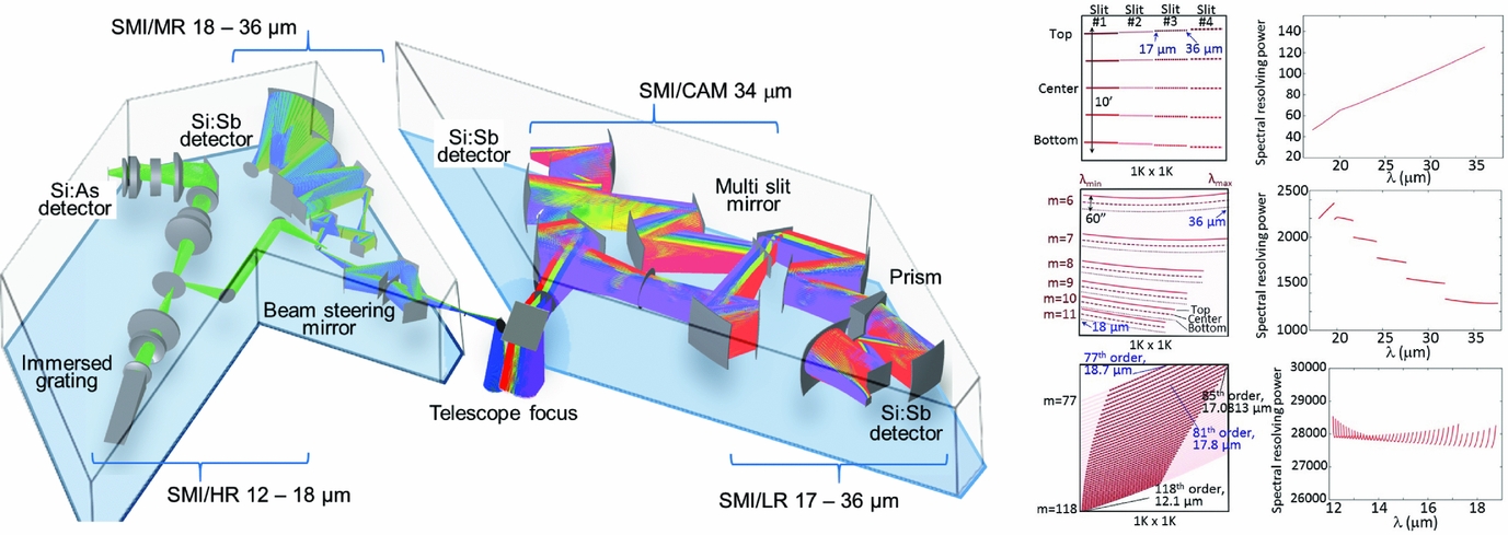
Figure 15. Left: optical layout for SMI/MR–HR and SMI/LR with SMI/CAM. The colour coding of rays is based on the angular positions in the fields-of-view. Right: Spectral formats and spectral resolutions of SMI/LR, SMI/MR, and SMI/HR (top to bottom).
As is the case for SMI/LR–CAM, the SMI/MR and SMI/HR share fore-optics, including a BSM. In combination with the telescope step-scan mode, for SMI/MR, the BSM provides access to a ~2 arcmin × 2 arcmin on-sky area. In the aft-optics, the beam is routed into either the SMI/MR or SMI/HR channels. SMI/MR has a long slit of 60 arcsec length and 3.7 arcsec width. The beam passes through this slit and collimating optics, and is subsequently dispersed by an echelle grating combined with a cross-disperser. The resulting 18–36 μm spectrum, spread over six different orders from m = 6 to 11 (middle panel of Figure 15 right panel).
SMI/HR has short, 4-arcsec length, 1.7-arcsec wide slit. It employs a CdZnTe immersed grating and a cross-disperser to disperse the signal from the slit, and collimating optics before the beam reaches the Si:As array. One part of the spectrum is obtained in 34 high orders (85th to 118th) covering 12.14 to 17.08 μm, and a second part in eight lower orders (77th to 84th) partly covering the 17.08 to 18.75 μm range (Figure 15, right bottom panel).
3.2.2. The SMI detector arrays
SMI employs two kinds of photoconductor arrays, Si:Sb 1 K×1 K and Si:As 1 K×1 K detectors. Figure 16 shows the quantum efficiencies that has been achieved by these types of detectors as a function of the wavelength. To achieve this performance, the detectors must be operated at low temperatures: <2.0 K for Si:Sb and <5.0 K for Si:As. Three Si:Sb arrays are used to cover wavelengths >17 μm (SMI/LR–CAM and SMI/MR) and one Si:As array for wavelengths below 18 μm (SMI/HR). Si:As has heritage from previous space missions such as AKARI/IRC, Spitzer/IRAC and IRS, WISE and JWST/MIRI. To date, Si:Sb has been used only for Spitzer/IRS with a 128 × 128 array format. Development is planned for the Si:Sb arrays towards 1 K × 1 K arrays with improved quantum efficiency at longer wavelengths.
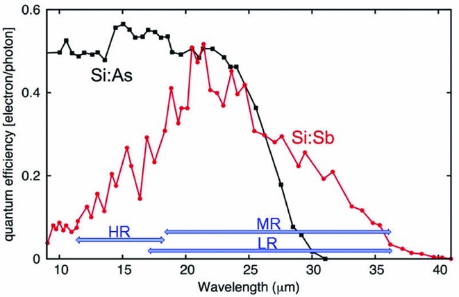
Figure 16. Quantum efficiency for Si:As (JWST/MIRI; Ressler et al. 2008) and Si:Sb (test model for SMI; Khalap et al. 2012) arrays that are currently available. The SMI wavelength range is shown in blue.
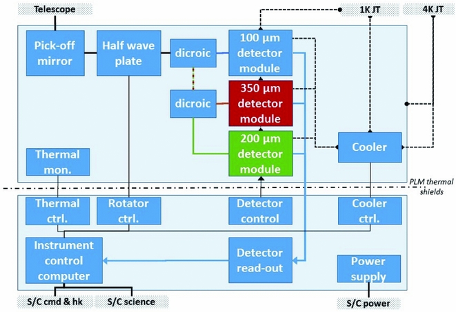
Figure 17. POL functional block diagram, implementing individual direction of three wavelength bands onto a common focal plane assembly. An achromatic half-wave plate in the common part of the optics train is used by all bands.
3.2.3. Observing with SMI
SMI has four nominal modes of observation: a staring mode, an SMI/LR mapping mode, an SMI/LR–CAM survey mode, and an SMI/MR mapping mode. The staring mode is used for targeted spectroscopy of point sources with SMI/LR–CAM, SMI/MR, or SMI/HR. In this mode for SMI/MR and SMI/HR, dithering or mapping of a small area is possible using the BSM. The SMI/LR mapping mode is used to perform slit scanning spectroscopy with SMI/LR to generate a full 10 arcmin × 12 arcmin spectral map with 90 scans each separated by a step of 2 arcsec. The survey mode is used for wide-area surveys with SMI/LR–CAM in which the spacecraft is scanning with steps of ~10 arcmin of the 10 arcmin × 12 arcmin field. The SMI/MR mapping mode is used for spectral mapping of extended sources by combining raster step scans and BSM movement.
3.3. A camera/polarimeter—POL
The prime science driver for a far-infrared polarimetric imaging function is the mapping of polarisation in dust filaments in our Galaxy, requiring a high dynamic range both in spatial scales and flux density. Efficient mapping requires an instantaneous field-of-view which is as large as possible and viewed simultaneously in different wavelength bands. Thus, detectors are required that offer good sensitivity at faint flux levels, but are not affected by high flux levels. The wavelength bands for POL are defined by the need to observe filaments on both sides of their peak emission, and centred around 100, 200, and 350 μm. For efficient polarimetry, polarising detectors are used. The specifications of the instrument are summarised in Table 4; a block diagram is shown in figure 17. The adopted detector sensitivity of 3 × 10⁻¹⁸ W √Hz−1 can be achieved with detectors which were originally developed for an earlier incarnation of the SAFARI spectrometer.
Table 4. POL performance parameters.
3.3.1. The POL optics
The instrument optical layout is shown in Figure 18, it employs common entrance optics for the three bands, providing field and aperture stops for stray light suppression as well as a pupil image for the half-wave plate, followed by individual branches for the three wavelength bands. The half-wave plate is an achromatic design, providing nearly constant phase shift across the entire wavelength range. The plate is operated at 4.8 K and it is immediately followed by a 1.8 K Lyot stop. All further elements are inside a 1.8-K enclosure. After the intermediate focus/field stop, light is re-collimated and split into the three wavelength bands by means of two dichroic filters. The collimated beams in the three separate bands are re-focused onto the three detector arrays with different magnification, to match physical pixel sizes and optical point spread functions at the band centre wavelengths. A boundary condition for the optics design has been to align the three detector focal planes close enough in position and orientation to allow their integration in one common FPA at 50 mK. Band-defining filters are mounted on the 300 and 50-mK levels of the FPA. To optimise between sensitivity, mapping speed, and resolution, a 1.22/2Fλ pixel size is used.
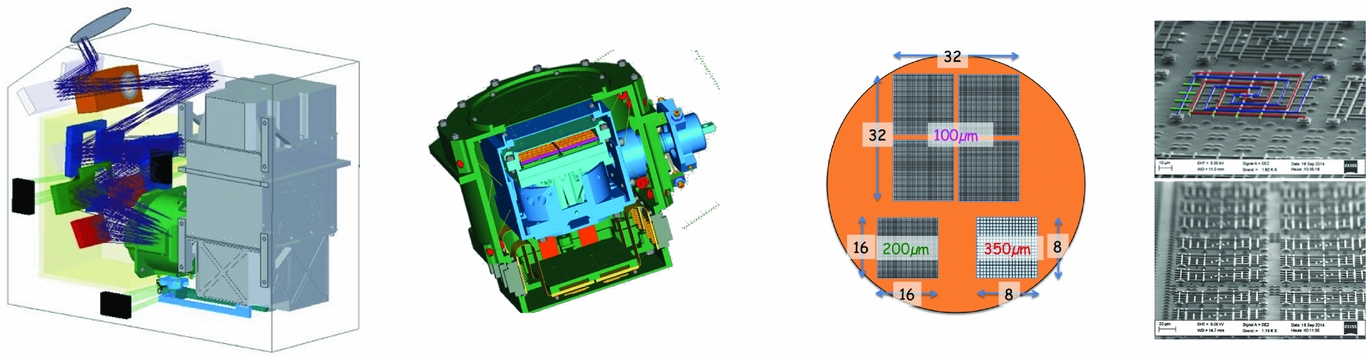
Figure 18. POL focal plane unit, detector assembly, and detectors. Left: The three band layout of POL. Right: The FPA structure—light blue indicates the 50-mK stage, dark blue the 300-mK stage, and green the 1.8-K stage. The two inner stages are suspended by Kevlar wires. Right top: A single POL pixel showing an interlaced grid of small metallic vertical and horizontal polarisation absorbers on an Si substrate. These ‘antennae’ absorb one polarisation of the incoming radiation and the power dissipation results in temperature changes in the support structure. These changes are sensed using the four spiral arm thermistor leads—two of the leads couple to the structure supporting the horizontal polarisation antennae, and two to the vertical polarisation. Right bottom: An array of the POL pixels.
The instrument requires an actuator for the half-wave plate at the 4-K temperature level. An electromagnetic motor design based on the Herschel/PACS (Poglitsch et al. Reference Poglitsch2010) filter wheels or the more compact motor used in FIFI–LS (Klein et al. Reference Klein2014) on SOFIA (Becklin et al. Reference Becklin, Young and Savage2016) can be used. To minimise dissipation during movements, an integrated wheel/motor design is foreseen, as the main dissipation occurs not in the motor coils but by mechanical friction in the bearings of the mechanism. The half-wave plate is rotated only between scans, and its operation will contribute marginally to the thermal load on the 4-K-JT stage.
3.3.2. The POL detector assembly
The detector assembly (see Figure 18) holds three detector ensembles, one for each spectral band. The 100-μm band has four 16×16 pixel modules butted in a 2×2 configuration, the 200-μm band has one 16×16 pixel module, and the 350-μm band one 8×8 module. All modules have the same physical size, ~20 mm, and the same field-of-view.
The detector assembly is a ‘Russian dol’ structure at 1.8 K with two suspended stages. The innermost level at 50 mK houses the six detector modules and is thermally linked to the 50-mK cryocooler tip by a light-tight coaxial pipe. The 50-mK level is enclosed in a 300-mK box linked to the cryocooler by the same cooling pipe. POL will use the same cooler design as SAFARI. To prevent out-of-band stray light, the beam passes through filters at the entrance to each enclosure.
To achieve sufficient dynamic range, semiconductor bolometers are used, with heritage from the Herschel PACS bolometer arrays, redesigned to support polarisation measurement (Figure 18), and cooled to 50 mK to achieve the required sensitivity. These resistive sensors do not show any saturation with absorbed power, but they do suffer from a non-linear response. This non-linearity can be taken in account by applying a proper calibration over a wide range in incident power.
The bolometer detector consists of two suspended interlaced spirals, each sensitive to a single polarisation component. The metallic absorbers (here dipole antennae matched to vacuum impedance) form a resonant cavity with a reflector on the readout circuit surface. The cavity is partially filled with a dielectric (SiO) to tailor the detector bandwidth. The front-end readout circuit also operates as a buffer stage output for the time domain multiplexing function, both operating at 50 mK. The multiplexing leads to a large reduction in the number of connections to the coldest stage, minimising the thermal load. The large difference in dynamic range between total power and polarisation is addressed by the use of a Wheatstone bridge configuration. The three Stokes parameters (I, Q, and U) can in principle be retrieved simultaneously in the PSF by a ‘polka dot’ configuration with every other detector rotated by 45°. Nevertheless, a half-wave plate located at the instrument entrance is necessary to disentangle scene polarisation from instrumental self-polarisation.
3.3.3. Observing with POL
The foreseen operating mode of the detectors will produce a combined, total power, and difference signal for two orthogonal polarisations. For simple imaging, any mapping scheme can be used. For polarimetry, the default observing mode will be scan maps, along with two approximately orthogonal scan directions. The scan map will be repeated with one or more different orientations of the half-wave plate. The wave plate serves two purposes: It provides access to the π/4 and 3π/4 orientations and allows the removal of polarisation effects introduced by the instrument by swapping the two orthogonal polarisations of the detector. To establish reliable end-to-end characterisation of the polarisation properties of the complete system (telescope plus instrument), calibration observations will be repeated at regular intervals during the mission.
4 SPICA OPERATIONS
4.1. Launch and operations
SPICA is envisaged to be launched into space on JAXA’s next-generation H3 launch vehicle from the JAXA Tanegashima Space Centre. The satellite will be directed to a halo orbit around the Sun–Earth Libration point 2 (S-E L2) which provides a stable thermal environment. The orbit will give access to a 360° annulus with a width of about 16° on the sky, providing full sky access over a 6-month period (see Figure 19). Most the cosmological fields of interest have good visibility (over 40 d yr−1), deep observations of fields like COSMOS and UDS likely will require re-visits over multiple years. For galactic sources, the visibility varies, unfortunately with somewhat poorer visibilities for some of the prototypical sites of galactic star formation like Taurus and Ophiuchus. The spacecraft will be operated in a 24-h cycle autonomous operation. In a daily contact period, a new 24-h schedule will be uploaded, while instrument and spacecraft data stored in mass memory will be downloaded.
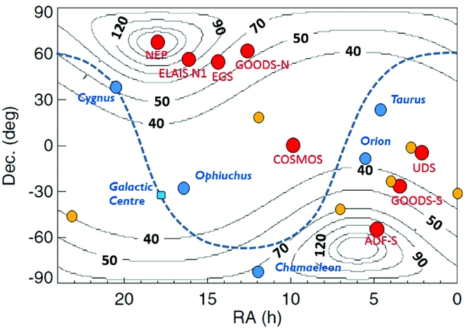
Figure 19. Sky visibility contours, in unit of days per year. Circles identify popular extragalactic survey fields (red), HST Frontier Fields (yellow), and Galactic star-forming regions (blue).
The spacecraft will be launched at an ambient temperature, and the payload will be cooled to the operating temperature in early mission operations. The lifetime required for the mission will be 3 yr, with a goal of 5 yr. Given the fact that mission lifetime does not depend on a limited cryogen supply, a further extension is quite conceivable; the cryogen-free design would allow extension of the mission lifetime beyond the nominal duration and is ultimately limited only by propellant and potential on-board hardware degradation. The different operational phases of the mission are indicated in Figure 20.
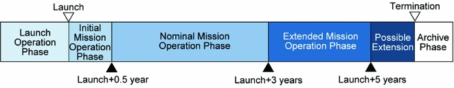
Figure 20. Operational phases of the SPICA mission.
4.2. Ground segment
The ground segment will be designed to run the mission such that its scientific harvest is maximised. It consists of the Mission Operation Centre (MOC), the Science Operation Centre (SOC), the Science Data Centre (SDC), and the Instrument Control Centres (ICCs). Figure 21 shows these centres together with the main flows of information.
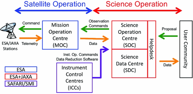
Figure 21. SPICA operational centres and information flow.
The MOC is responsible for all spacecraft operations including the execution of routine observations and contingency plans. It will monitor the health and safety of the spacecraft and instruments, and when needed to take corrective actions, and will generate and upload commands based on the observation plan input from the SOC and receive telemetry data. The MOC is expected to be operated in Europe (by ESA). The SOC will be in charge of the science operation of SPICA, i.e. the handling of observing proposals, generating schedules of approved science, and calibration observations for the MOC to generate and upload daily commands, and handling the downlinked science data. The SDC will develop and maintain the data reduction toolkit/pipeline software together with the ICCs. The data will be processed and archived by the SDC, and made available to the ICCs and science users. The SOC and SDC will jointly operate a help desk as a unique contact point for science users. The SOC and SDC will be established in the framework of collaboration between ESA and JAXA.
The ICCs, under the responsibility of the instrument teams, will work together with the SOC and the SDC to ensure that the focal-plane instruments are well calibrated and optimally operated. They will monitor instrument health, define and analyse calibration observations, and will also be responsible for developing and maintaining the scientific data reduction software.
4.2.1. Operation scheme
As soon as the fundamental spacecraft functions have been successfully verified, functional checkout of the focal plane instruments will start followed by the scientific performance verification (PV) phase. When warranted by the PV results, observing programmes may need to be adjusted to account for the established in-flight performance. The spacecraft will carry out observations autonomously, according to a timeline of commands uploaded from the ground. The baseline operational mode foresees no parallel mode operations—at any one time only a single instrument will be active.
Data taken by the instruments will be made available to the data owners for scientific analysis. In the routine phase, observation data will be delivered to the users within one month after successful execution of the observation. Calibration and data reduction software will be updated regularly during the operation. Major updates will be made available every 0.5–1.0 yr. All data will be re-processed by the SDC using the new pipeline.
4.3. Science programmes
SPICA is to be operated as an international observatory to accomplish the mission science goals as well as to execute science programmes proposed by the wider community. Two categories of observing programmes are foreseen: Key Programmes (KP: significant, consistent, and systematic programmes to carry out the mission’s prime science goals) and General Programmes (GP, all other observing programmes). Observing time will be divided into Guaranteed Time (GT: reserved for instrument consortia and other groups involved in developing the mission), Open Time (OT: open to the worldwide community), and Director’s Discretionary Time (DDT). For obvious reasons, a major part of the GT (>70%) shall be defined as KP.
Any programme proposed by consortium members (GT) or coming from the worldwide community (OT) could be a KP or a GP, depending on its goals and/or nature. A Time Allocation Committee (TAC) will review all observing time proposals and propose prioritised time allocations to the Scientific Advisory Board (SAB) on the basis of scientific merit. The SAB will subsequently ratify the observation programme with the priorities proposed by the TAC. It will also be the role of the SAB to define what should be the proportion of KP in the OT.
In the nominal 3-yr mission, the first six months will be used for cooling the telescope, and verification and validation of the observatory and its instruments. OT proposals will be assigned the largest fraction of the remaining 2.5 yr, while a more modest part (<40%) will be dedicated to GT and a small (<5%) part will be reserved as DDT. In a possible mission extension, the proportion of GT will be small (<10%), the DDT will remain the same (<5%) and most of the time will be OT open to the worldwide community. Figure 22 illustrates this concept for the time division over programme categories.
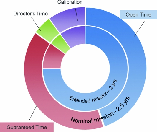
Figure 22. Division of observing time over different programme categories.
The SPICA project will be responsible for Level-2 processing of the data, i.e. correction for instrument-specific features and calibration to make the data ready for scientific analysis. All science data will be archived, and made publicly available after a proprietary period of 1 yr.
5 CONCLUSIONS
The joint European–Japanese infrared space observatory SPICA will provide a major step in mid- and far-infrared astronomical research capabilities after the Herschel mission. To minimise the background noise level, SPICA will employ a 2.5-m telescope cooled to below 8 K. As a result, the detectors are no longer affected by the thermal radiation coming from the mirror itself, allowing the ultrasensitive SPICA instruments to detect infrared sources over two orders of magnitude weaker than would have been possible with previous infrared space observatories.
The instrument complement foreseen for SPICA will provide extremely sensitive spectroscopic capabilities in the 12 to 230 μm domain with various modes in resolving power—ranging from extremely sensitive R = 300 spectroscopy instantaneously covering the full 34 to 230 μm band to a high resolution R ~ 28000 mode between 12 and 17 μm. In addition, large field-of-view sensitive imaging photometry at 34 μm and imaging polarimetry at 100, 200, and 350 μm is provided. The observatory cryogenic system is based on a combination of passive cooling and mechanical cryocoolers, making the operational lifetime independent of liquid cryogens.
With SPICA, astronomers wil, e.g. be able to study the process of galaxy evolution over cosmic time in much more detail and out to much larger redshift than was possible before. Furthermore, the observatory will allow detailed investigations into the process of planet formation, as well as the study of the role of the galactic magnetic field in star formation in the dust filaments.
ACKNOWLEDGEMENTS
This paper is dedicated to the memory of Bruce Swinyard and Roel Gathier. Bruce initiated the SPICA project in Europe, but sadly died on 2015 May 22 at the age of 52. He was ISO-LWS calibration scientist, Herschel-SPIRE instrument scientist, first European PI of SPICA and first design lead of SAFARI. Roel was managing director of SRON until early 2016 when he died after a short sickbed on 2016 March 14. Roel also was head of the Dutch delegation in the Science Programme Committee (SPC) and later SPC chairman. He was crucial in giving and generating support for the SPICA mission in the Netherlands, but also throughout Europe, Japan, and North America.
The SAFARI project in the Netherlands is financially supported through NWO grant for Large Scale Scientific Infrastructure nr 184.032.209 and NWO PIPP grant NWOPI 11004. The TES detector development work for SAFARI has received support from the European Space Agency (ESA) TRP program (contract number 22359/09/NL/CP).
FN and JTR acknowledge financial support through Spanish grant ESP2015-65597-C4-1-R (MINECO/FEDER).


