


1. Introduction
Powerful human-generated transmissions corrupt weaker radio signals from cosmic sources. Balancing the advantages of wireless communication, satellite navigation, consumer electronics, weather forecasting and air transport with novel techniques (Zheleva et al. Reference Zheleva2023) to manage Radio Frequency Interference (RFI) is essential in keeping scientific research in radio astronomy sustainable in the future. The challenge for radio astronomy is not only the comparative power of these unwanted signals but also their increasing prevalence (Committee on Radio Astronomy Frequencies 1997). From a scientific perspective, all undesired signals are described as RFI. However, practically (and legislatively) emissions are only classified as RFI if they impinge on the authorised user of bands allocated (or shared) amongst different services (e.g. the radio astronomy service (RAS), aeronautical radionavigation service, broadcasting service, fixed/mobile service, etc.). In Australia this is under the jurisdiction of the Australian Communications and Media Authority (ACMA), and of the International Telecommunication Union (ITU) treaty, implemented by way of the radio regulations (RRs) (Baan Reference Baan2019; ITU-R 2016). To further complicate the issue some RFI is a result of unintended electromagnetic radiation, emission outside the service allocation of the intended transmission and therefore not subject to the same regulations stipulated above (Di Vruno F. et al., Reference Di Vruno, Winkel and Bassa2023; Grigg D. et al., Reference Grigg, Tingay and Sokolowski2023).
There are many methods of RFI mitigation (Fridman & Baan Reference Fridman and Baan2001; Kesteven Reference Kesteven2010; Series Reference Series2013; Baan Reference Baan2019) depending on the type of RFI and instrument. Indeed, observatories have to use a variety of techniques at different stages in the signal chain to manage RFI (Baan Reference Baan2019). Flagging is the most common strategy to mitigate the effects of RFI in radio astronomy; it is the process of identifying and discarding corrupt data in the frequency or time domain. Flagging can be conducted manually but is increasingly done by more sophisticated flagging software (Offringa et al. Reference Offringa2010; Burd et al. 2018). Unfortunately, flagging reduces measurement sensitivity and the discarded data may contain valuable information from astronomical sources. Flagging also impacts the instrumental response in ways that may require consideration when drawing scientific conclusions. An example is that flagging impacts the UV coverage and thereby the point spread function of a synthesis imaging array like the Australian SKA Pathfinder (ASKAP). Furthermore, newer generations of radio telescopes with increased sensitivity, larger bandwidths, and wider fields of view – designed to keep up with contemporary science goals – are more severely affected by RFI, resulting in even more flagging.
The ASKAP telescope, operated by the CSIRO, is one such instrument (Hotan et al. Reference Hotan2021). ASKAP operates over the 700–1 800 MHz band of which less than 4% is allocated to the RAS on a primary basis in three small protected bands:
-
1. 1 400–1 427 MHz (Hydrogen line),
-
2. 1 610.6–1 613.8 MHz (OH line), and
-
3. 1 660–1 670 MHz (OH line).
The remainder of the frequencies ASKAP operates are in use by the fixed/mobile service, the radio location service, the aeronautical mobile service, the aeronautical radionavigation service, and the radionavigation-satellite service (ITU-R 2016; Indermuehle et al. Reference Indermuehle, Harvey-Smith, Wilson and Chow2017; AustralianCommunications and Media Authority 2021).
RAS has secondary allocation for spectral line observations from 1 718.8 to 1 722.2 MHz, and some minimal protection is afforded from 1 710 to 1 930 MHz via footnote 5.149 in the RR, stating ‘[.]administrations are urged to take all practicable steps to protect the radio astronomy service from harmful interference’ (ITU-R 2016). The radio spectrum is therefore a finite resource supporting a diversity of vital services. Current and future radio telescopes operating in large bandwidths outside of the RAS protected bands, where usage purely for astronomy purposes is not possible, need to monitor, and coexist with other services.
ASKAP is comprised of $36 \times 12$
m antennas with a 188-element checkerboard phased array feed at the focus of each dish, allowing up to 36 independent dual-polarisation beams to be formed on the sky (Hotan et al. Reference Hotan2021). The maximum separation between antenna pairs (baseline length) is approximately 6 km. Because low RFI environments are required for radio astronomy, the ASKAP telescope was built about 600 km northeast of Perth, at Inyarrimanha Ilgari Bundara, the CSIRO Murchison Radio-astronomy Observatory. State and federal legislation has established a protected area known as the Australian Radio Quiet Zone – Western Australia (ARQZWA) established by ACMA (Wilson, Storey, & Tzioumis Reference Wilson, Storey and Tzioumis2015; Wilson et al. Reference Wilson2016), a circular region of 260 km radius from the observatory centre. However, the regulation does not protect ASKAP from orbiting satellites (of particular concern for the planned deployment of several low earth orbit mega-constellations), air traffic navigation, or mobile communication towers outside the ARQZWA. The latter of which cause interference during tropospheric ducting events. Ducting is an anomalous propagation phenomenon that can cause the refractive index of the atmosphere to match that of the curvature of the earth and thereby enables radio waves to refract and travel much farther than usual (Hall & Barclay Reference Hall and Barclay1989; Indermuehle et al. Reference Indermuehle, Harvey-Smith, Wilson and Chow2017).
$36 \times 12$
m antennas with a 188-element checkerboard phased array feed at the focus of each dish, allowing up to 36 independent dual-polarisation beams to be formed on the sky (Hotan et al. Reference Hotan2021). The maximum separation between antenna pairs (baseline length) is approximately 6 km. Because low RFI environments are required for radio astronomy, the ASKAP telescope was built about 600 km northeast of Perth, at Inyarrimanha Ilgari Bundara, the CSIRO Murchison Radio-astronomy Observatory. State and federal legislation has established a protected area known as the Australian Radio Quiet Zone – Western Australia (ARQZWA) established by ACMA (Wilson, Storey, & Tzioumis Reference Wilson, Storey and Tzioumis2015; Wilson et al. Reference Wilson2016), a circular region of 260 km radius from the observatory centre. However, the regulation does not protect ASKAP from orbiting satellites (of particular concern for the planned deployment of several low earth orbit mega-constellations), air traffic navigation, or mobile communication towers outside the ARQZWA. The latter of which cause interference during tropospheric ducting events. Ducting is an anomalous propagation phenomenon that can cause the refractive index of the atmosphere to match that of the curvature of the earth and thereby enables radio waves to refract and travel much farther than usual (Hall & Barclay Reference Hall and Barclay1989; Indermuehle et al. Reference Indermuehle, Harvey-Smith, Wilson and Chow2017).
An holistic strategy to manage the effects of RFI, must include legislation, spectrum management, cooperation, avoidance, flagging, and active RFI mitigation (Hellbourg et al. Reference Hellbourg, Weber, Capdessus and Boonstra2012; Black et al. Reference Black, Jeffs, Warnick, Hellbourg and Chippendale2015; Hellbourg, Bannister, & Hotarp Reference Hellbourg, Bannister and Hotarp2017) but also continued monitoring and evaluation of RFI’s impact on the observatory (Indermuehle et al. Reference Indermuehle, Harvey-Smith, Wilson and Chow2017). To this end, observatories and telescopes have started to perform statistical analysis of flagging data (Offringa et al. Reference Offringa2015; Zhang et al. Reference Zhang2021; Sihlangu, Oozeer, & Bassett Reference Sihlangu, Oozeer and Bassett2021). In this paper, we present our analysis of 1 MHz resolution flagged data from the ASKAP radio telescope’s data processing pipeline as a function of frequency and time. Section 2 describes ASKAP’s data products and processing as well as the RFI environment at the observatory. Section 3 describes the implementation of the flagged statistics pipeline. We present an analysis of the effect of RFI on ASKAP science, based on over 1 500 h of ASKAP observations in Section 4. Finally, future work and concluding remarks are presented in Sections 5 and 6, respectively.
2. ASKAP data and inferring RFI through flagged data
The data collected for this project is fromprocessed and archived ASKAP continuum observations from April 2019 to August 2023. Archived ASKAP visibilities are stored with 1 MHz frequency channels and 10 s integration time resolution. ASKAP Survey Science Projects (SSPs) typically observe over three ‘clean’ bands, below 1 085, 1 293–1 437 MHz (excluding 1 149–1 293 MHz severely impacted by radion avigation-satellites which is observed but discarded before processing) and above 1 510 MHz, which we refer to as the ‘clean’ low, mid and high bands, respectively. For a full description of ASKAP, including the technical specifications and overview of science operations, seeThe data collected for this project is fromprocessed and archived ASKAP continuum observations from April 2019 to August 2023. Archived ASKAP visibilities are stored with 1 MHz frequency channels and 10 s integration time resolution. ASKAP SSPs typically observe over three ‘clean’ bands, below 1 085 MHz, 1 293–1 437 MHz (excluding 1 149–1 293 MHz severely impacted by radion avigation-satellites which is observed but discarded before processing) and above 1 510 MHz, which we refer to as the ‘clean’ low, mid, and high bands, respectively. For a full description of ASKAP, including the technical specifications and overview of science operations, see Hotan et al. (Reference Hotan2021).
ASKAP operates primarily as an automatically scheduled telescope to carry out observations, with the autonomous scheduler SAURON (Scheduling Autonomously Under Reactive Observational Needs) communicating to the telescope operating system (TOS, Guzman & Humphreys Reference Guzman and Humphreys2010) via parameter specifications (Hotan et al. Reference Hotan2021, Moss et al. in preparation). SAURON conducts system and environment checks as part of the scheduling decision-making, but RFI is largely not included as a factor. The exception to this is ducting avoidance, where some SSPs have elected to not to observe if there is active ducting due to the impacts on data quality (mainly loss of sensitivity or bandwidth coverage).Footnote a Observations for these SSPs are not scheduled during active ducting, and if ducting starts during an observation, SAURON will interrupt the observation. Further discussion on the severity of ducting is presented in Section 4. The other most problematic sources of RFI are relatively consistent, meaning that active avoidance has not been necessary. The dramatic rise in solar activity approaching the solar maximum (and observed impacts on ASKAP calibration and science data) are likely to result in more active consideration of solar activity as part of future upgrades to SAURON. Similarly, it has been discussed whether active satellite avoidance as a constraint may be beneficial to especially the mid band observations, but to date the SSPs and observatory have instead elected to remove the RFI-corrupted lower 144 MHz bandwidth from 1 149 to 1 293 MHz. Work is currently underway as part of the Collaborative Intelligence Future Science Platform collaboration to implement machine learning anomaly detection on ASKAP raw data diagnostics. This work will identify and characterise outliers in the data, including RFI, and it is expected that the first version of this will be in production before the end of 2023. Note that while RFI due to increased solar activity does negatively affect science observations and operations, it does not trigger the flagger and therefore the results presented here are not accounted for by solar interference.
The ASKAPsoft pipeline (Guzman et al. Reference Guzman, Chapman, Marquarding and Whiting2016; Cornwell et al. Reference Cornwell2016) is the collection of software required to process ASKAP data end-to-end including calibration, ingest, flagging, averaging, imaging, source-finding and archiving. ASKAP data is processed at the Pawsey Supercomputing Centre where each of ASKAP’s 36 beams are processed in parallel (Hotan et al. Reference Hotan2021). There are two processes in the pipeline involved in flagging. First, before the data is averaged to 1 MHz, known RFI is excised based on an RFI database, and then on-the-fly detection and excision occurs (Cornwell et al. Reference Cornwell2016). The RFI database used, is an internally developed table of known transmitters affecting the observatory (Indermuehle et al. Reference Indermuehle, Harvey-Smith, Wilson and Chow2017). Averaged coarse-resolution 1 MHz data may be flagged again before being imaged and archived (Hotan et al. Reference Hotan2021). Flaggers generally use fixed and dynamic thresholds in amplitude (or using circular polarisation) to remove anomalous samples in the calibrator and science data. This approach works because many sources of RFI have amplitudes much higher than the noise and astronomical signal (McConnell et al. Reference McConnell2020). Weak noise-like RFI, however, can still be missed in the flagging process. The default flagging algorithm embedded in the ASKAPsoft pipeline is CFLAG (CSIRO 2022), but the specification parameters also allow the alternative use of AOFLAGGER (Offringa et al. Reference Offringa2010; Offringa, Van De Gronde, & Roerdink Reference Offringa, Van De Gronde and Roerdink2012). Resulting data products from ASKAPsoft are stored in the CSIRO ASKAP Science Data Archive (CASDA)Footnote b (Chapman et al. Reference Chapman, Lorente, Shortridge and Wayth2017; Huynh et al. Reference Huynh, Dempsey, Whiting, Ophel, Ballester, Ibsen, Solar and Shortridge2020).Flagging data is stored alongside visibility data in CASA-style Measurement Sets (Hotan et al. Reference Hotan2021; Kemball & Wieringa Mark 2000). ASKAPsoft also outputs diagnostic and quality information throughout the pipeline, including a summary of flagged data per observation.
Our research builds on the existing flag summary reports generated by ASKAPsoft. We establish a baseline of flagged data against which to compare and predict the expected amount of flagged data. We also contribute to the body of research outlining the RFI environment at the observatory (Offringa et al. Reference Offringa2015; Tingay et al. Reference Tingay, Sokolowski, Wayth and Ung2020; Sokolowski, Wayth, & Lewis Reference Sokolowski, Wayth and Lewis2016; Indermuehle et al. Reference Indermuehle, Harvey-Smith, Wilson and Chow2017) and recreate a statistical approach to monitoring of RFI flagging which is becoming more widespread in largescale telescope operations. Offringa set al. (2015) describes the low-frequency environment at the observatory using ten nights of Murchison Widefield Array (MWA) data. Similar approaches at other observatories, include Zhang et al. (Reference Zhang2021) with the Five-hundred-meter Aperture Spherical radio Telescope (FAST) in China using approximately 300 h across 45 days, and in South Africa using the MeerKAT telescope where Sihlangu et al. (Reference Sihlangu, Oozeer and Bassett2021) implemented a counter-based solution (which we have also used) using approximately 1 500 h of data. Flagging statistics can be used to monitor long-term changes in the RFI environment, monitor spectrum compliance, and improve the planning of observations such that the impact of RFI is minimised. Finally, this work will inform the ongoing development of active RFI mitigation (Black et al. Reference Black, Jeffs, Warnick, Hellbourg and Chippendale2015; Hellbourg Reference Hellbourg2016; Chippendale & Hellbourg Reference Chippendale and Hellbourg2017) and subsequently monitor the efficacy of these techniques (Hellbourg et al. Reference Hellbourg, Weber, Capdessus and Boonstra2012) in reducing flagging.
3. Approach and implementation: flagstats
We have used flag tables to infer the effects of RFI on ASKAP science and to monitor changes in the RFI environment as a function of frequency and time. We developed software to routinely extract, aggregate, analyse and visualise flagged data from ASKAP in near real-time. We opted for a bespoke software solution to systematically aggregate and analyse flagged data because to our knowledge, no compatible open-source software existed. As such, we created the flagstats library based on available Python libraries and existing scripts in ASKAP’s pipeline that interrogate ASKAP measurement sets and summarise flagged data. The flagstats library is broken into four main components StatsWriter, StatsReader, StageStats and StatsGUI. Fig. 1 shows the high-level sequence of those components as well as their input and output data products.
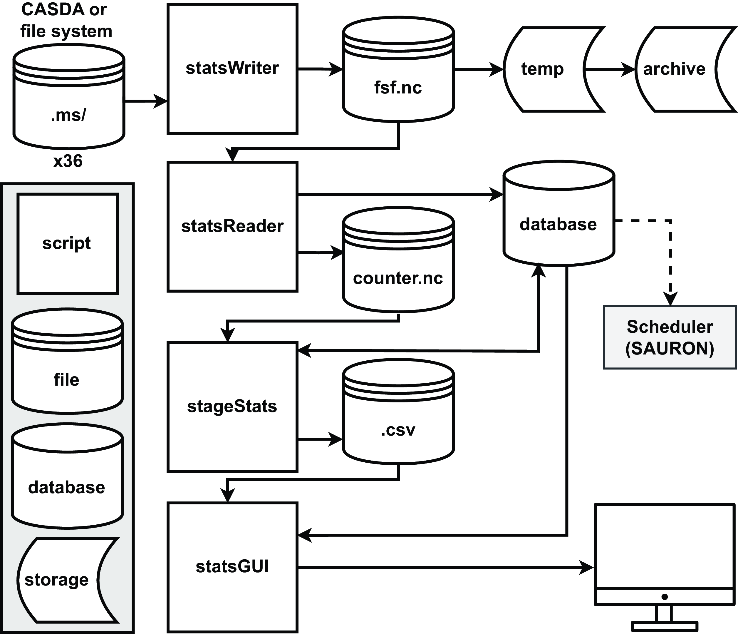
Figure 1. Components of the flagstats library and their data inputs and outputs. StatsWriter extracts flags, StatsReader aggregates them, StageStats further aggregates, performs analysis, and prepares files that serve the GUI, statsGUI for interactive visualisation of flags and aggregated data.
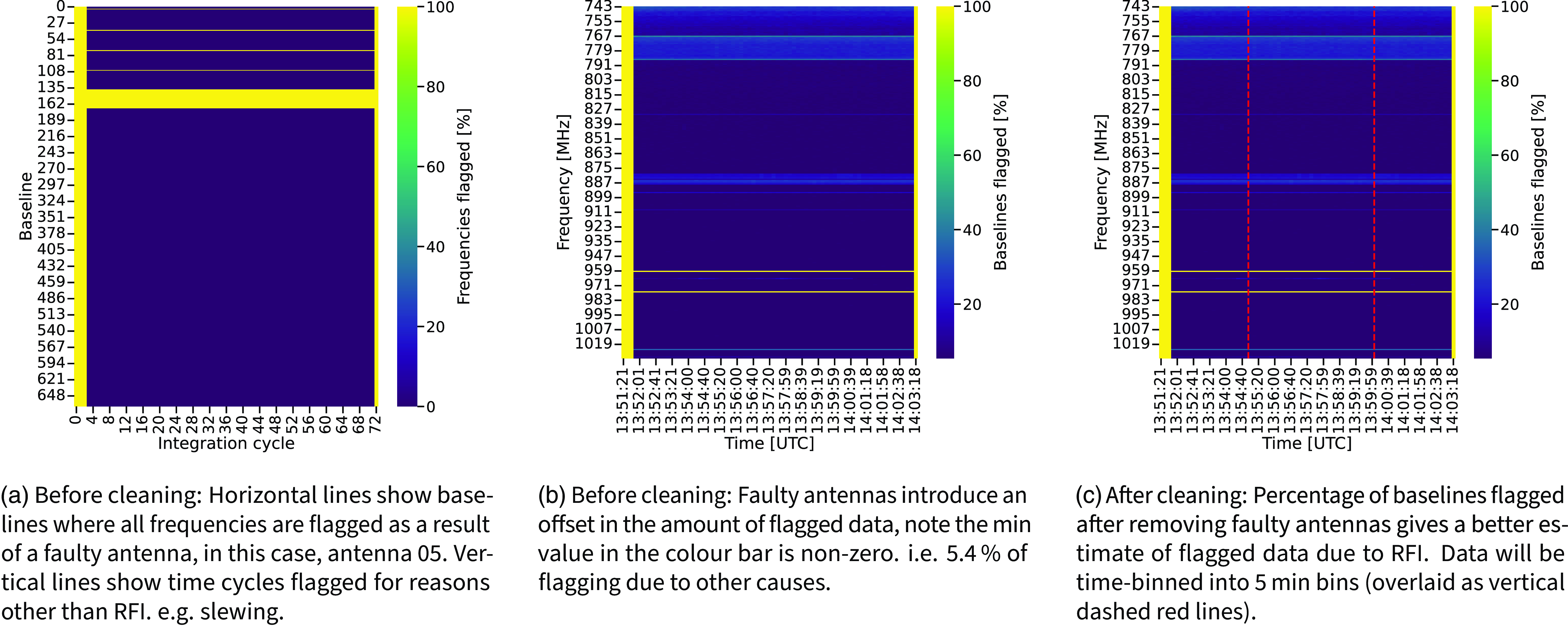
Figure 2. Sub-figures (a) and (b) show the flag cube before removing faulty antennas. (c) shows the ’cleaned’ cube with a more accurate estimate of flags due to RFI.
StatsWriter
StatsWriter takes a set of ASKAP measurement sets as an input and outputs a file containing the flagging tables from each beam for the duration of the observation and relevant metadata extracted using dask-ms.Footnote c Flagging for all four polarisation products (XX, XY, YX, and YY) are recorded in the original measurement set, but, flagging across polarisations is currently the same for ASKAP, therefore to reduce the size of the output only the XX polarisation flagging table is stored. A benefit of having these relatively smaller individual flagsummary.nc Footnote d files (per observation) is that users can query them to get comprehensive statistics about the flagging (and RFI) affecting a specified observation using StatsReader.
StatsReader
StatsReader is the key component of the flagstats library. It first cleans (removes non-RFI-related) flagged data stored in the previous step. A series of ‘counter’ files are created if they do not exist. Data is binned for each observation, in turn. The appropriate counter is updated to aggregate flagged data from multiple observations. Counters from which statistics are computed are updated with the flagged and total number of contributing samples of each bin similar to Sihlangu et al. (Reference Sihlangu, Oozeer and Bassett2021).
Consider a single beam from an ASKAP observation, where the flag table from the measurement set is reshaped and stored into a 3-dimensional array of shape, $n_{\text{freq}} \times n_{\text{cycles}} \times n_{\text{baselines}}$
. Fig. 2a shows the percentage of flagged frequency channels in the observation as a function of time (in integration cycles) on the x-axis and baseline on the y-axis. Fig. 2b, is the same cube but shows the percentage of flagged baselines in the observation as a function of time (in UTC) on the x-axis and 1 MHz frequency channels on the y-axis. We call Fig. 2a and b the ‘dirty’ cube because faulty and intermittent antennas have not yet been removed. ASKAP currently uses boolean flags which are True when the data is discarded/flagged. One of StatsReader’s functions is to identify (and remove) flags that are not due to RFI. The vertical yellow lines in Fig. 2a show time cycles for which all frequency channels are flagged, similarly horizontal lines show baselines for which all frequency channels are flagged throughout the observation. For the latter, an antenna can be mapped to a set of baselines due to a faulty antenna(s), in this case antenna ak05. For the former, flags are from timing issues (slewing time if all antennas are not in the ‘tracking’ state and latency of data flow through the digital systems). StatsReader will disregard flags where all frequencies are affected over either all baselines or all integration cycles because they are not from RFI. StatsReader also cleans antennas that ‘drop out’ mid-observation.
$n_{\text{freq}} \times n_{\text{cycles}} \times n_{\text{baselines}}$
. Fig. 2a shows the percentage of flagged frequency channels in the observation as a function of time (in integration cycles) on the x-axis and baseline on the y-axis. Fig. 2b, is the same cube but shows the percentage of flagged baselines in the observation as a function of time (in UTC) on the x-axis and 1 MHz frequency channels on the y-axis. We call Fig. 2a and b the ‘dirty’ cube because faulty and intermittent antennas have not yet been removed. ASKAP currently uses boolean flags which are True when the data is discarded/flagged. One of StatsReader’s functions is to identify (and remove) flags that are not due to RFI. The vertical yellow lines in Fig. 2a show time cycles for which all frequency channels are flagged, similarly horizontal lines show baselines for which all frequency channels are flagged throughout the observation. For the latter, an antenna can be mapped to a set of baselines due to a faulty antenna(s), in this case antenna ak05. For the former, flags are from timing issues (slewing time if all antennas are not in the ‘tracking’ state and latency of data flow through the digital systems). StatsReader will disregard flags where all frequencies are affected over either all baselines or all integration cycles because they are not from RFI. StatsReader also cleans antennas that ‘drop out’ mid-observation.
Fig. 2c shows the same cube but masked, that is, without the bad integration cycles and antennas, that we refer to as the ‘clean’ cube, which yields a better upper estimate of the flags due to RFI. Using the Radio Regulations (ITU-R 2016), spectrum plan (Australian Communications and Media Authority 2021), and known RFI affecting ASKAP (Indermuehle et al. Reference Indermuehle, Harvey-Smith, Wilson and Chow2017) we can map features in Fig. 2c to likely sources of RFI. It should be noted however that the 1 MHz frequency resolution is coarse compared to the bandwidth of many interferers, limiting the accuracy with which we can map flags to services. Furthermore, multiple interferers may also affect the same 1 MHz channel. Brighter horizontal lines in Fig. 2c show channels for which more (or all remaining) baselines/antennas are affected by RFI. Two red vertical dashed lines demarcate the three bins that this observation would be divided into. Starting from the top of the plot, this 12 min observation is corrupted by mixed fixed cellular interference below 787 MHz (Indermuehle et al. Reference Indermuehle, Harvey-Smith, Wilson and Chow2017). In the frequency range of this observation, there are many mobile base stations that routinely trigger CFLAG due to ducting, discussed further in Section 4 (see Fig. 9). For example, we know of two Vodafone base stations (identified by decoding RFI monitoring equipment) that operate in a frequency range of the affected channels in Fig. 2c (Indermuehle et al. Reference Indermuehle, Harvey-Smith, Wilson and Chow2017): the first in the Northampton Shire, 267 km south-west of ASKAP and the second in Carnarvon, 357 km north-west of ASKAP. In this case 960 MHz, like the 976 MHz flagged channel above it, the origin of the RFI is likely self-generated
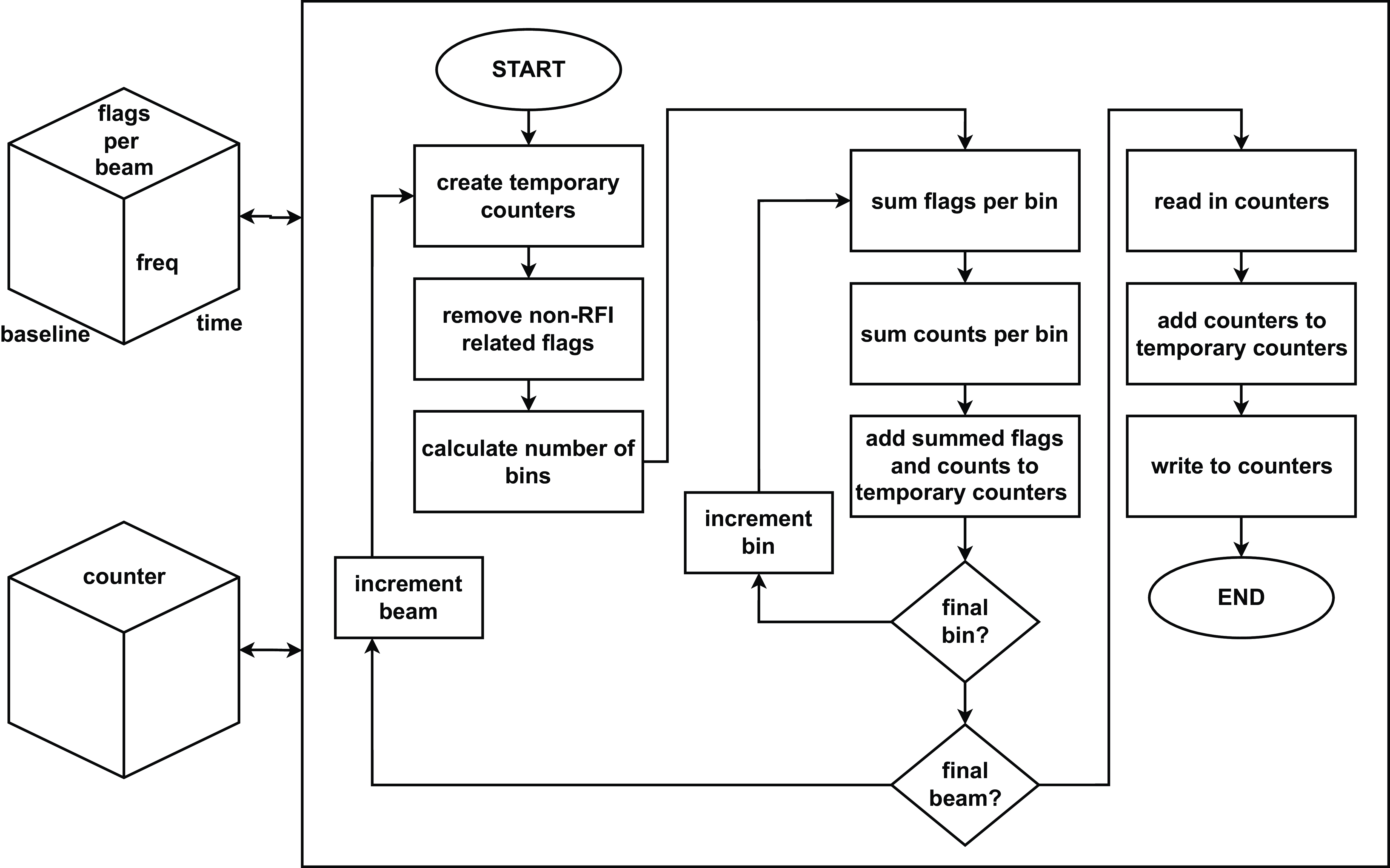
Figure 3. StatsReader takes an array of each beam’s flags in turn, creates a counter if one does not already exist, cleans the flag cube, bins the data, and updates the appropriate counter. This process is repeated for every observation. There are counters for all permutations based on the metric calculated, year and data source (science, bandpass, and RFI survey). Science data is further divided by the different Survey Science Projects (SSPs) processed (EMU, POSSUM, RACS, VAST).
An overview of the steps involved in StatsReader for an arbitrary counter are depicted in Fig. 3. Each counter.nc file has three groups,Footnote e one for each of the following counters:
-
The flag counter, tallies flags flagged as True, per bin.
-
the count counter, tallies the total number of samples per bin, that is, flagged as True or False.
-
The int_time counter, scales the count by the integration time of each observation to keep track of the flagging per unit time (typically represented in hours but stored in minutes).
We have implemented a series of counters as opposed to a single counter (Sihlangu et al. Reference Sihlangu, Oozeer and Bassett2021). First, for each metric we want to interrogate, there are individual counter files:
-
Time of Day, arrays in this counter have shape $1\,100 \times 666 \times 288$
:
$1\,100 \times 1 \textrm{ MHz}$
frequency bins, 666 baseline pairs from ASKAP’s 36 antennas and
$288 \times 5\,\textrm{min}$
time bins in a day. Fig. 2c shows these bins with two red vertical dashed lines.
$1\,100 \times 666 \times 288$
:
$1\,100 \times 1 \textrm{ MHz}$
frequency bins, 666 baseline pairs from ASKAP’s 36 antennas and
$288 \times 5\,\textrm{min}$
time bins in a day. Fig. 2c shows these bins with two red vertical dashed lines. -
Day of Week, arrays in this counter have shape
$1\,100 \times 666 \times 168$
; frequency, baseline, and 168
$\times$
1 h time bins in a week. -
Week of Year, arrays in this counter have shape
$1\,100 \times 666 \times 53$
; frequency, baseline, 52 complete weeks in a year and one incomplete week. Week zero is the week inclusive of the 4
$^{\textrm{th}}$
of January using the ISO week date system.


The above set of counter files is created for each permutation of year and type of data. SSP are further divided by the different surveys processed: EMU, POSSUM, RACS, VAST (see Section 4). StatsReader uses metadata stored in the extracted flags by StatsWriter to locate and update the appropriate counter files. This approach makes it easy to add new metrics, types of data or surveys by simply adding the associated counters. In addition to aggregating, cleaning, binning and updating counters, Fig. 1 shows that StatsReader writes high-level data, per observation to a database table. This table is used to keep track of the observations processed and includes the percentage of total flagged data (including bad antennas), percentage of flagged data due to RFI, duration, field of observation, data source, and survey name. At this point, counters per metric for each observation are aggregated in their respective counters – by year, type of data, and science survey – but not aggregated with each other.
StageStats
In order to create aggregated statistics for each metric, across different years, surveys and observing modes, counters of the same type must be added together. First, vertically, the counters created and updated by StatsReader in the lowest directory of the file hierarchy are added together by StageStats and placed at the level of the file structure above it until there is one counter per metric per year. Then counters are added horizontally until there is one counter per metric per type of data. Finally, counters from every year are added together. StageStats has three other processes:
-
Create tables from these ‘top-level’ counters and store them in the database with local copies to serve the GraphicalUser Interface (GUI).
-
Calculate high-level statistics based on the files processed by StageReader (Table 1). We also use this database table to infer observations affected by ducting, based on excess flagging.
-
Perform analysis of the aggregated data (see Section 4):
-
1. Compare flagging between day and night (Fig. 8).
-
2. Aggregate data from RFI monitoring equipment.
-
3. Compare flagged and RFI monitoring equipment data.
-
4. Map flagged data to corresponding radio service(s).
-
5. Calculate losses per service (Fig. 6).
-
6. Calculate losses per service year-on-year (Fig. 7).
-
7. Infer observations affected by ducting based on ‘excess’ flagging.
Finally, StageStats summarises statistics per metric (time of day, week, and year), to reduce the computation required for the interactive GUI.
StatsGUI
The StatsGUI is an interactive GUI. that allows users to explore aggregated flagged data. It also matches RFI probabilities to radio services and known transmitters in the same 1 MHz channel using a click callback. Users first select a metric to view (by default it is ‘time of day’), they can then use a series of filters to select data from a particular year, survey and/or observation type. We are in the process of automating the individual parts of the flagstats library. So far StatsWriter is fully implemented to extract flags from all bandpass and continuum science observations as soon as the processing is completed.
Automation
The ASKAP telescope is increasingly becoming an autonomous system building upon SAURON, a dynamic observation scheduling system (Moss et al. in preparation), and Process Manager, an event-based triggered workflow manager. Process Manager has been designed to allow the automatic triggering of a data processing pipeline (e.g. calibration and imaging) when a set of defined criteria have been met. We used the Python package prefect Footnote f to create an extensible workflow that implements the StatsWriter routines, which was then registered with Processing Manager and configured to trigger against all science observations once they have been processed by the larger ASKAP processing-pipeline. Hence, the flagging statistics that are currently extracted are from the calibrated measurement sets after the automated RFI flagging within the ASKAP processing pipeline have been performed. We plan to further develop our own prefect-based pipeline to directly run flagging procedures against the raw uncalibrated measurement set before they are processed by software in the larger ASKAP ecosystem. This improvement will gather useful statistics on sub-bands that are currently removed at the beginning of the ASKAP pipeline containing excessive RFI and therefore affecting scientific processing, for example over the frequency range 1 149–1 293 MHz impacted by the radionavigation-satellite service. While we continue to test, develop, optimise, and automate the software it remains internal, but we intend to explore options to generalise and make it more widely available as we further develop the software. In the next section, we present the preliminary results based on 1 MHz flagged data.
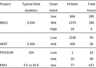
Table 1. Hours of continuum science data by processed Survey Science Project and band.
4. Results
In this paper, we present results based on science observations with at least 250 h per year from April 2019 to August 2023.Footnote g Flags from archived science data were collected via CASDA. Recent science data were directly processed from the Pawsey Supercomputing Centre file system. Most recently this is done automatically by triggering StatsWriter upon completion of the ASKAP processing pipeline. Table 1 shows the total observing time and number of observations of science data subdivided by survey and clean band. Science data from the following SSPs and their respective pilot surveys have been included:
-
the Rapid ASKAP Continuum Survey (RACS) I, II, and RACS-mid (McConnell et al. Reference McConnell2020; Hale et al. Reference Hale2021; Duchesne et al. Reference Duchesne2023),
-
the ASKAP survey for Variables and Slow Transients (VAST) (Murphy et al. Reference Murphy2013, Reference Murphy2021),
-
the POlarisation Sky Survey of the Universe’s Magnetism (POSSUM) (Anderson et al. Reference Anderson2021) and,
-
the Evolutionary Map of the Universe (EMU) (Norris et al. Reference Norris2011)
A key outcome of this work is shown in Fig. 4. Using the flagstats library, the data in Table 1 was extracted, cleaned, binned, aggregated, summed across SSP, data category, and metric and analysed. Fig. 4 shows the probabilities of flagging due to RFI as a function of frequency and time of day. The x-axis, binned to 5 min, is given in Coordinated Universal Time (UTC) in the format hh:mm.
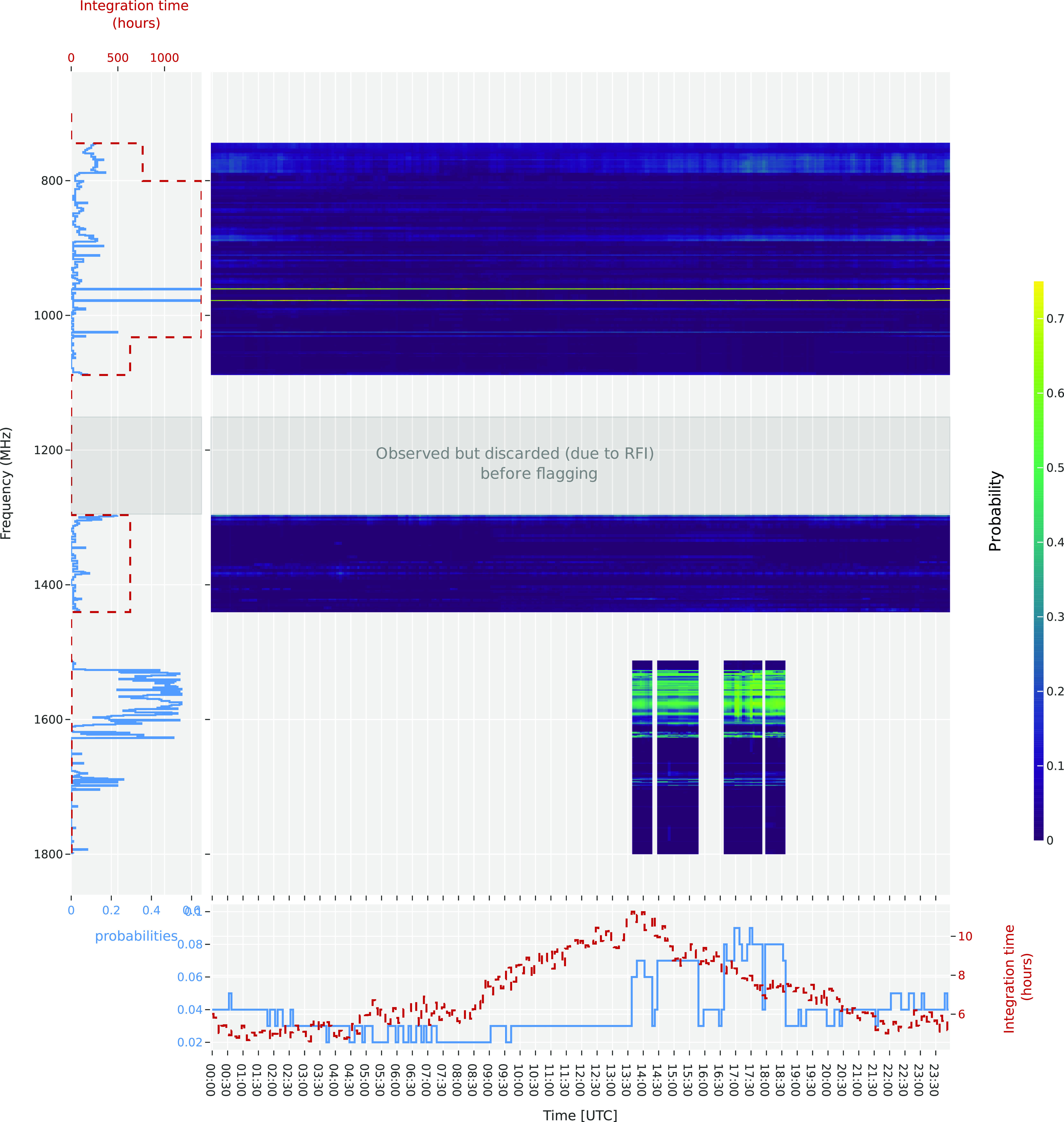
Figure 4. The central heatmap shows the probability of flagging due to RFI based on the aggregation of over 5 000 scheduling blocks comprising approximately 1500 h of observing time from April 2019 to August 2023. The x-axis is binned to 5 min, and the y-axis to 1 MHz frequency channels. The vertical subplot to the right shows the average flagging due to RFI in blue as a function of frequency. Similarly, the horizontal subplot at the bottom shows the average flagging due to RFI as a function of the time of day in blue. The red curves in both subplots show the number of hours that contributed data to that bin. Three sub-bands in which ASKAP continuum observations are most typically conducted are shown. From top to bottom, the low band shows flagging due to RFI from the fixed/mobile service exacerbated by ducting, the two most prominent peaks are likely due to self-generated interference in ASKAP’s signal chain. Aeronautical mobile and radionavigation affect the low and mid bands shown above. Note the bottom half of the mid band from 1 149 to 1 293 MHz whilst observed is not processed or archived as it is severely affected by radionavigation-satellites. The lower half of the high band is affected by various satellite services, in addition the high band is affected by meteorlogical aids and satellite services as well as fixed/mobile. Both the mid and high bands have protected radio astronomy service allocations for HI and OH spectral lines, respectively.
The y-axis shows ASKAP’s 1 MHz resolution frequency channels in ascending order. The vertical subplot to the left shows the average flagging due to RFI across the day as a function of frequency in blue. Similarly, the horizontal subplot at the bottom shows the average flagging due to RFI across the ASKAP band as a function of the time of day in blue. Both subplots show the contributing number of observing hours per bin in red.
An upper estimate on the total percentage of flagged data due to RFI across ASKAP’s frequency range is is 3%. Starting from the lowest frequencies and working upwards, we will discuss the corresponding primary service allocations (Australian Communications and Media Authority 2021) to features in Figs. 4 and 8.
Figs. 4 and 8 show flagging below 787 MHz, and around 841, 884, and 894 MHz which are most likely attributable to the closest mobile base stations operating at those frequencies (see Fig. 9). Flagged data above 960–1 163 MHz range is likely due to aeronautical radionavigation. The end of ASKAP’s clean low band (1 085 MHz) terminates where RFI due to aeronautical radionavigation is expected to increase based on measurements by RFI monitoring equipment (middle panel, Fig. 8).
Radionavigation-satellite routinely affect the 144 MHz below 1 293 MHz, although observed, this sub band is discarded before processing result in a large section of bandwidth in which no flagging data has been collected. The clean mid band from 1 293 to 1 437 MHz is affected by flagging in corresponding to the following services: radio location service for use by the Australian Defence Force and Department of Defence from 1 300 to 1 400 MHz and the RAS hydrogen line protected band from 1 400 to 1 427 MHz in which the strong hydrogen line emission itself may be triggering CFLAG.
Various satellite services affect the bottom half of the high band (1 510–1 797 MHz) including radionavigationsatellite satellite and radiodetermination-satellite services as well as aeronautical radionavigation. The RAS OH spectral line protected band from 1 610.6 to 1 613.8 MHz and 1 660 to 1 670 MHz is located between the above satellites and meteorlogical aids and satellite services and fixed/mobile which fills the remainder of ASKAP’s frequency range.
ASKAP self-generated RFI
Not all RFI is external to the observatory and telescope, with ASKAP itself (and the infrastructure supporting it) capable of generating RFI, which might include power supplies and electronic components. Self-generated RFI is generally unintended and we aim to identify and ultimately reduce the impact of these unwanted sources of RFI caused within the observatory.
An example of this in early ASKAP observations/operations is the On-Dish Calibrator (ODC) a noise source used for calibrating the Phased Array Feed (PAF) which introduced RFI (particularly in the shortest, baselines, and in the low part of the band). The ODC is now only switched on as needed, during the beginning of beamforming and before an observation to update the weights, not during the observation. The ODC is designed to be broad-band and operates at about 1% of the system temperature. It is therefore unlikely to have caused any additional flagging. Furthermore, the majority of data presented herein was collected after this issue was resolved. Shielding is also used to mitigate the effects of RFI in the observatory control building. In some cases due to planned activities at the observatory (including maintenance and construction), the risk of RFI is increased. In these instances a Radio Emissions Management Plan (REMP) is conducted to prevent and avoid RFI as much as possible.
Another example includes some digital artefacts that impact the data like RFI but can be coherent across the array without being radiated into it due to their originating from coherent clock signals. A dominant example is a 256 MHz clock that is multiplied by 32/27 to read out the digital receiver’s 1 MHz resolution oversampled coarse filter bank (Tuthill et al. Reference Tuthill2012; Brown et al. Reference Brown2014). Table 2 shows calculated values of harmonics of this clock signal and frequencies that they will appear at in observations due to the direct sampling architecture of ASKAP’s digital receiver. This clock signal is narrowband and correlated across antennas.
Table 2. Calculated interference due to harmonics from $32/27 \times 256$
MHz coarse filterbank readout clock in ASKAP’s digital receiver. Bolded frequencies are potentially triggering the flagger, strikethrough text indicates frequencies outside the available ASKAP observing band. Apparent frequencies calculated for direct sampled filter bands as defined in Brown et al. (Reference Brown2014).
$32/27 \times 256$
MHz coarse filterbank readout clock in ASKAP’s digital receiver. Bolded frequencies are potentially triggering the flagger, strikethrough text indicates frequencies outside the available ASKAP observing band. Apparent frequencies calculated for direct sampled filter bands as defined in Brown et al. (Reference Brown2014).
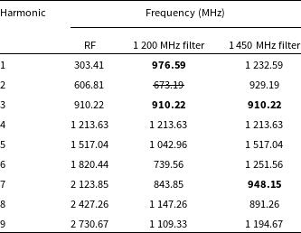
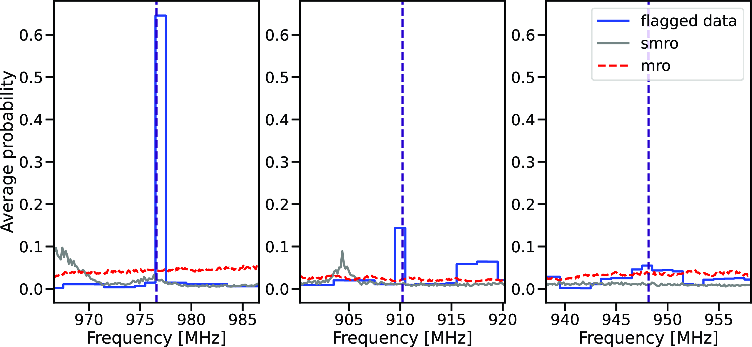
Figure 5. Mapping flagged data at the calculated harmonics of self-generated interference, overlaid are the probabilities of RFI based on the RFI monitors. For these frequencies there is no externally measured RFI but flagging, consistent with self-generated interference.
This signal is internal to each digital receiver card and is well shielded inside ASKAP’s shielded room. It enters the signal path directly on the digitiser cards. Note the 673.19 MHz value has been struck through because it is outside of ASKAP’s observing range and therefore does not see corresponding flagging in the data collected herein.
Fig. 5 shows how by using the values in Table 2 we map the probabilities of flagging due to RFI to frequencies that are likely flagged due to self-generated interference. that is, the bolded frequencies in Table 2 are potentially triggering the flagger. The flagged data from Fig. 4 is shown in Fig. 5 as a solid blue step plot, with step widths of 1 MHz. Overlayed and with a higher frequency resolution, are two separate RFI monitors used at the observatory, the first (solid grey) and the second (dashed red). The first is more sensitive owing to its slower scanning rate and thus longer integration time (‘s’ stands for sensitive in the name). It is better suited for detection of faint signals often seen from satellites, distant transmitters such as mobile base stations (See Fig. 8), and localised weak electromagnetic interference. The faster and thus less sensitive RFI monitor is paired with an active antenna to make up in part for the faster scan rate. Both scan from 20 to 3 000 MHz, the first has finer frequency resolution, 3.125 kHz, with a sweep time of 62 s, compared to the second which scans at 100 kHz with a sweep time of 1.49 s, permitting detection of rapid transient emissions. More information on RFI monitoring equipment can be found in Indermuehle et al. (Reference Indermuehle, Harvey-Smith, Wilson and Chow2017). The point is that at the frequencies with flagging peaks in Fig. 5 and no corresponding measurement by the RFI monitoring equipment, we detected three self-generated RFI candidate frequencies on which to follow up. There is a mechanism in the ASKAPsoft injest software, ‘on-the-fly averaging’ based on an amplitude threshold, that should remove the underlying narrowband signal causing CFLAG to flag these 1 MHz channels; we believe these candidates are not strong enough to trigger this mechanism and are therefore subsequently flagged. An additional candidate signal of this nature not previously documented, the 960 MHz flagged channel in Figs. 4 and 8 has been identified for further investigation.
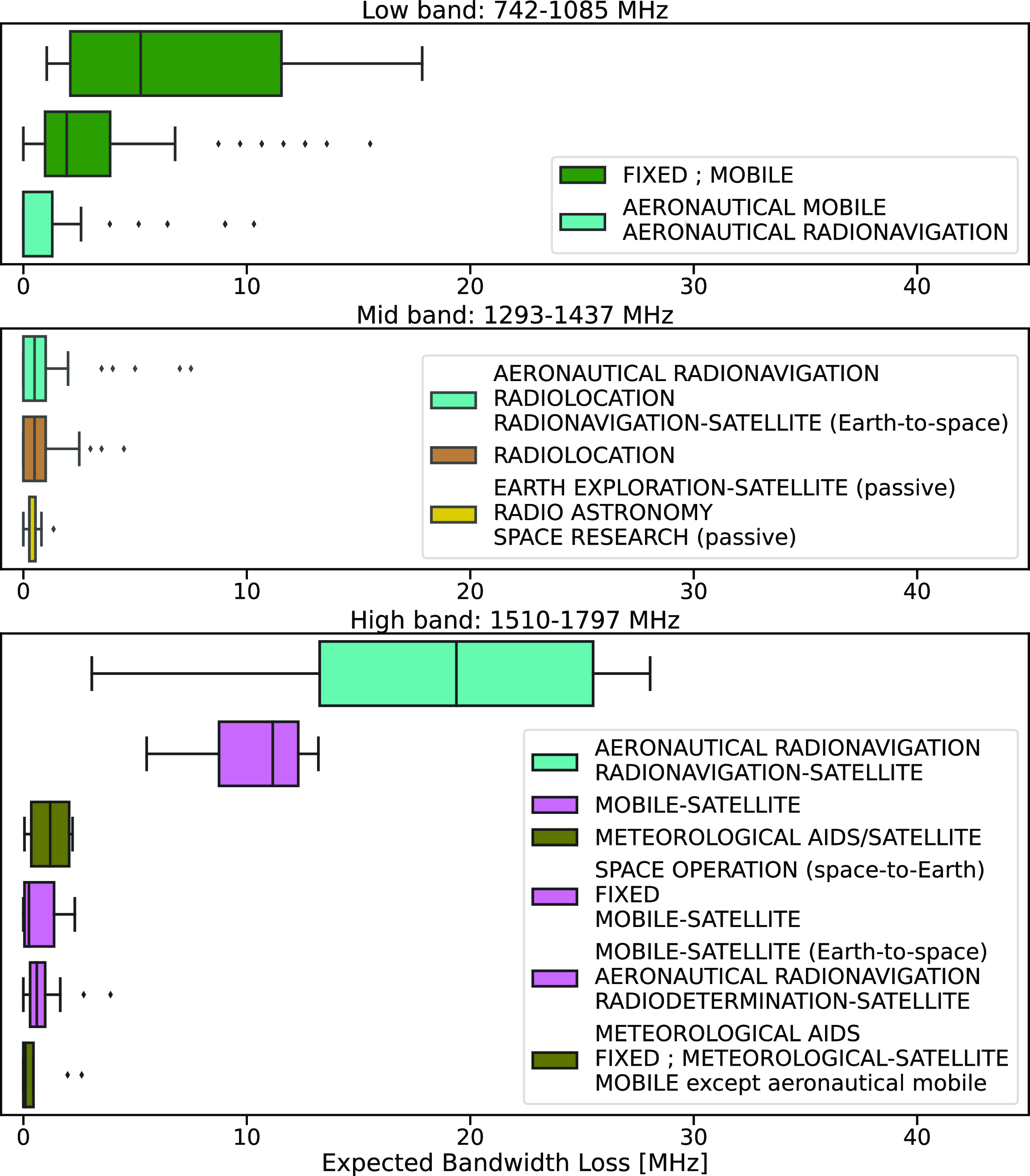
Figure 6. An estimated bandwidth loss is calculated by multiplying the channel width (1 MHz) by the probability of flagging in that channel and summing all the channels corresponding to a particular primary service allocation. For each band – ASKAP’s low (top panel), mid (middle panel) and high (bottom panel) bands – the estimated bandwidth loss of the highest average flagged services are shown. The mid band (excluding radionavigation-satellite affected data) is the least affected by RFI followed by the low and high bands. The low band is most affected in fixed/mobile (green) allocations and the high band by aeronautical (cyan) and satellite allocations (pink).
RFI-affected science data
The elevated steps in the red vertical subplot of total integration time in Fig. 4 (where we have accumulated more data) identify two clean bands that ASKAP regularly observes in the low and mid bands. Across the science bands flagging due to RFI is 3%.
The average flagging in the low band is 5% and is mostly accounted for by four primary service allocations.
Less than 0.1 MHz is lost to RFI in this band without identification of a corresponding primary service allocation. The top panel of Fig. 6 shows the two primary service allocations that most affect the low band are both fixed/mobile allocations (green) to which combined ASKAP science loses between 6 and 20 MHz. Estimated losses are calculated by multiplying the channel width (1 MHz) by the probability of flagging in that channel and summing all the channels corresponding to that service resulting in a range of expected/estimated bandwidth losses in MHz.
The average mid band flagging is 1%. This does not include the 144 MHz below 1 293 MHz discarded before processing 100% of the time which is affected by radionavigationsatellites. Including this would increase the total flagging due to RFI across all bands to 15%. The remainder of the mid band (as it appears in CASDA) is the least affected by flagging due to other sources of RFI. Three primary service allocations correspond to this band. The middle panel of Fig. 6 shows that no more than 2 MHz across 75% of the most affected channels is lost to flagging due to RFI. The three most prevalent sources of flagging correspond to transmitters in the aeronautical radionavigation, radio location and earth exploration satellite primary service allocations. ASKAP’s mid band is of particular importance as it contains the biggest protected RAS allocation centred on the 1 420 MHz hydrogen line. In this allocation up to 0.4 MHz is lost due to flagging; that is, 1.5% data in the hydrogen line protected RAS allocation is flagged.
We compared the estimated losses to the measured RFI monitoring occupancy, that is the average percentage of detected RFI in a channel using the RFI monitoring equipment since 2019. We find that in general, across the clean bands there is more agreement between ASKAP and the more sensitive RFI monitor. Both RFI monitors find fixed/mobile to be the most significant cause of interference in the low band. RFI monitoring equipment does however detect more interference due to aeronautical mobile and radionavigation service related interference compared to ASKAP flagging data. Similarly, in the mid band there is alignment between services and the more sensitive RFI monitor. More high-band observations are required to make reliable comparisons with RFI monitoring equipment.
RFI trends
Several other trends in the probabilities of flagging due to RFI based on Fig. 4 were also explored including the expected bandwidth loss per service year-on-year, differences in the probability of flagging due to RFI in the day compared to night and the effects of ducting as compared to RFI monitoring equipment.
Year-on-year
Following on from the previous section, the estimated bandwidth loss per service can be further separated by year. There is only enough data to make this comparison in ASKAP’s clean low and mid bands, shown below for a subset of primary spectrum services.
Fig. 7 again shows that the clean mid band is less affected by RFI than the low band. In the low band, we see again that the primary losses are due to fixed/mobile (green). The data also shows that there is a year-on-year increase in the amount of flagged data corresponding to fixed/mobile allocations. Interestingly, in the RFI monitoring data this trend is not evident, which could suggest that the amount of interference year-on-year remains more or less constant, but since 2019 the ASKAP pipeline has improved in identifying and flagging the interference. Fig. 7 shows less flagging in the bands corresponding to aeronautical radionavigation service allocations (cyan) in 2019 and 2020, compared to after 2020 consistent with travel restrictions due to the COVID-19 pandemic. This pattern is not as clear in the mid band aeronautical radionavigation service allocations, nor do we see any obvious increases in the modest flagging in any other services. Of concern are the (yellow) protected RAS allocations where in previous years there have been non-negligible losses. Further investigation is required using full resolution data from the ‘Survey and Monitoring of ASKAP’s RFI environment and Trends’ (SMART) project to determine if in some cases CFLAG is flagging the 21 cm line itself or if this is due to RFI as a result of unintended electromagnetic radiation.
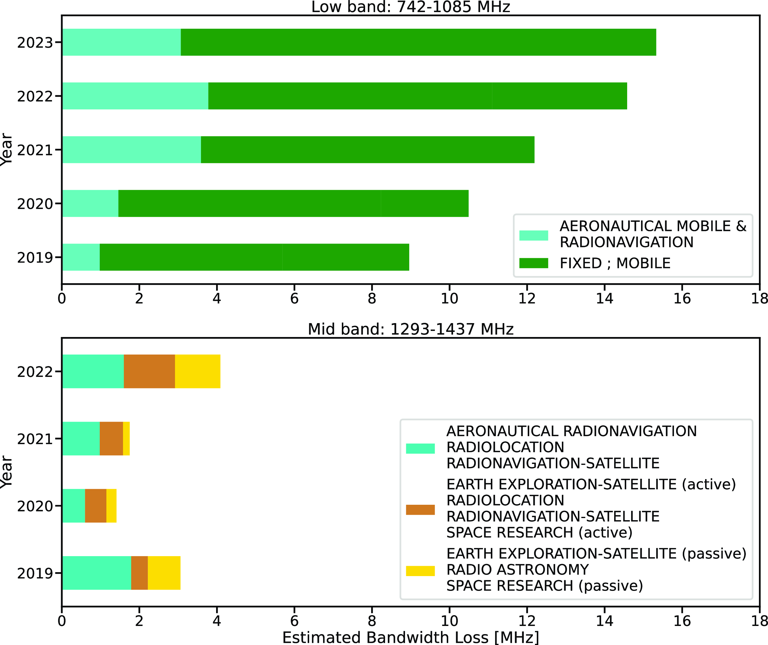
Figure 7. For the low band (top panel) and mid band (bottom panel), there is enough data to determine trends in the estimated bandwidth loss per service year-on-year. The increasing losses corresponding to fixed/mobile (green) is of concern in the low band. The (yellow) protected RAS allocations in the mid band where in previous years there have been non-negligible losses require ongoing monitoring and investigation to asertain the source of the flagging.
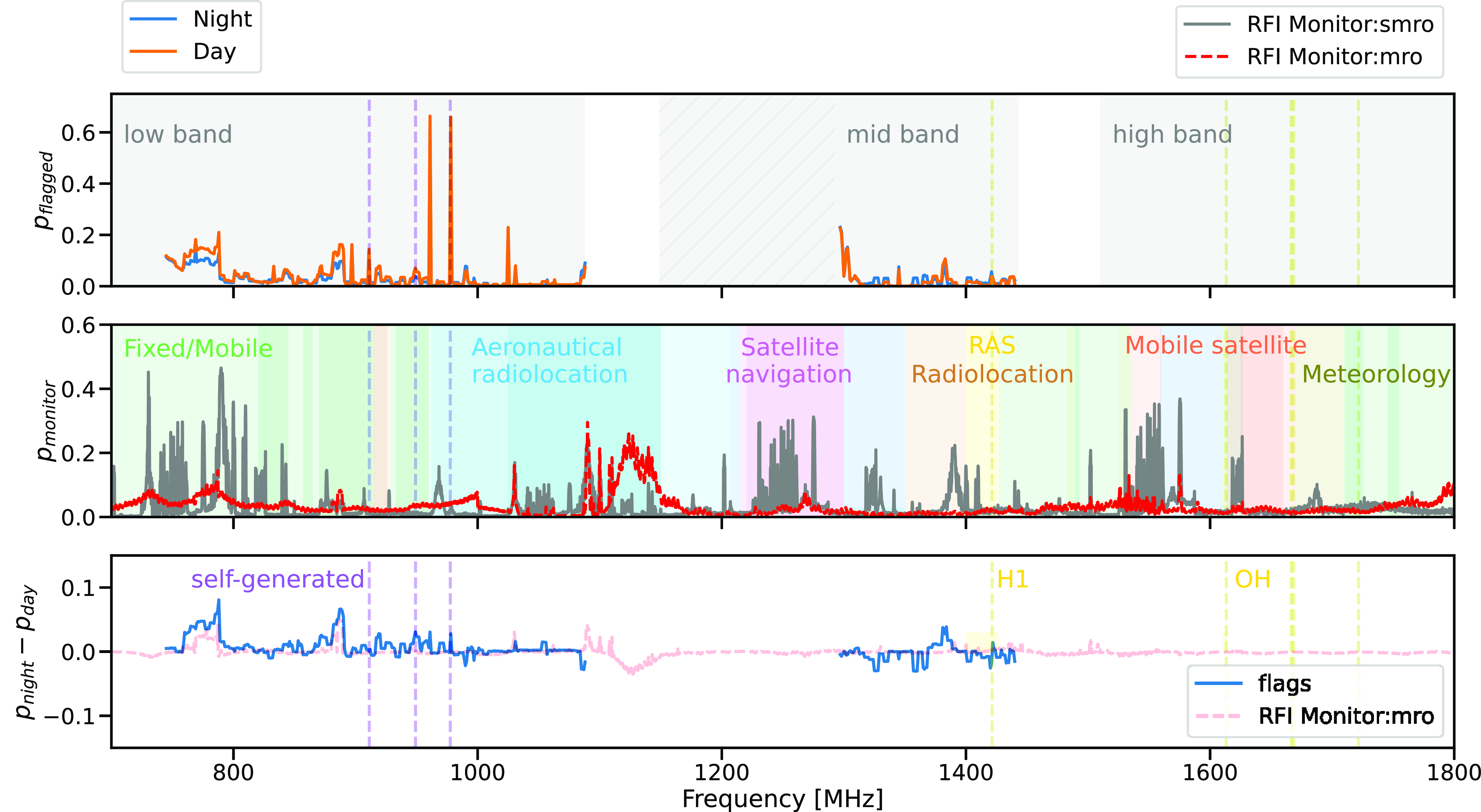
Figure 8. The top panel shows the mean probability of flagging, (from the blue vertical subplot in Fig. 4) comparing flagging in the day (orange) versus night (blue). The middle panel shows the probability of RFI based on RFI monitors. The bottom panel shows differences in flagging between night and day (blue) and RFI monitor (opaque red dashed curve in the background). In the background of the top panel are ASKAP’s low, mid, and high bands (hatched area is discarded after observing). In the background of the second panel the broad ranges of several primary allocations affecting ASKAP. Finally, the protected band (spectral lines) in yellow and the self-generated RFI in purple are shown vertically across all panels.
Day vs Night
Fig. 4 shows some variation as a function of day and night. The red curve on the horizontal subplot is the easiest to discern by eye. Historically, it indicates that there have been more continuum science observations between 08:00 and 21:00 UTC (16:00 and 03:00 local time). This trend can be explained by maintenance on-site and beamforming occurring during the day. Going forward with full survey operations we expect this difference to be reduced. Note, ASKAP does not currently support SSPs being observed only at night. Another obvious variation between day and night is in the main plot below 800 MHz and at 900 MHz corresponding to the fixed/mobile service which shows more flagging after sunset (19:00 local time 11:00 UTC).
To quantitatively determine the variations between day and night, Fig. 8 plots probabilities due to RFI in the day (orange) and night (blue) as a function of frequency in the top panel; that is, the blue vertical subplot in Fig. 4 split into flagging in the day versus night. We have defined the daytime as 06:00 to 18:00 local time (inclusive) based on the average sunset and sunrise times across the year corresponding to 22:00 to 10:00 UTC in Fig. 4. This division also yields two equal 12 h subsets of data with which to make the comparison. The middle panel in Fig. 8 shows the probability of RFI based on two RFI monitors at the observatory with different integrating times. The smro (solid grey) RFI monitor is more sensitive to transmission from mobile base stations and satellites, the mro (dashed red) RFI monitor gives better estimates on transmission from aeronatical radionavigation equipment, for example Distance Measuring Equipment (DME). The bottom panel shows the difference between day and night in flagging (blue) and the mro RFI monitor (red). The ranges of the clean low, mid and high bands are shown in the background of the top panel. The ranges of several primary radio allocations affecting ASKAP are also shown in the middle panel. The RAS protected bands and spectral lines are shown in yellow. Finally, the candidate self-generated RFI signals from Fig. 5 are overlayed vertically across all three panels in purple.
The bottom panel in Fig. 8 shows variations in flagging between day and night (the solid blue curve) are within $\pm$
10%. This curve traces the mro RFI monitor. Positive values in the bottom panel indicate that the interference and flagging are worse at night and negative values indicate the interference and flagging are worse during the day. The most prominent examples of variations between day and night are in the low band, the fixed/mobile below 800 MHz and at around 870 MHz is more likely during the night. At first one might expect that RFI due to cellular interference would decrease at night when people are generally asleep. However, recall that ASKAP is located in the ARQZWA, this means that RFI from mobile base stations (see Fig. 9) is more likely to affect ASKAP during ducting events. Indeed, upon comparison with RFI monitoring ducting predictors since 2019, ducting is 9% more likely on average at night.
$\pm$
10%. This curve traces the mro RFI monitor. Positive values in the bottom panel indicate that the interference and flagging are worse at night and negative values indicate the interference and flagging are worse during the day. The most prominent examples of variations between day and night are in the low band, the fixed/mobile below 800 MHz and at around 870 MHz is more likely during the night. At first one might expect that RFI due to cellular interference would decrease at night when people are generally asleep. However, recall that ASKAP is located in the ARQZWA, this means that RFI from mobile base stations (see Fig. 9) is more likely to affect ASKAP during ducting events. Indeed, upon comparison with RFI monitoring ducting predictors since 2019, ducting is 9% more likely on average at night.
Ducting
We have tried to identify the percentage of scheduling blocks affected by ducting based on ‘excess’ flagging compared to the mean across all scheduling blocks. Table 3 shows the percentage of scheduling blocks per band with probabilities greater than the mean, $1\sigma$
and
$1\sigma$
and $2\sigma$
above the mean. Across all data, day and night, and across all seasons we estimate an upper limit of 12% of the processed scheduling blocks affected by ‘excess’ flagging potentially due to ducting. There are not yet any discernible seasonal trends in ‘excess’ flagging though, across the year. Sokolowski et al. (Reference Sokolowski, Wayth and Lewis2016) observed ducting in 28% of 131 nights in summer at the observatory at low frequencies (
$2\sigma$
above the mean. Across all data, day and night, and across all seasons we estimate an upper limit of 12% of the processed scheduling blocks affected by ‘excess’ flagging potentially due to ducting. There are not yet any discernible seasonal trends in ‘excess’ flagging though, across the year. Sokolowski et al. (Reference Sokolowski, Wayth and Lewis2016) observed ducting in 28% of 131 nights in summer at the observatory at low frequencies ( $\leq$
300 MHz), with which we expect some correlation during periods of intense ducting at ASKAP’s frequency range (Indermuehle et al. Reference Indermuehle, Harvey-Smith, Wilson and Chow2017).
$\leq$
300 MHz), with which we expect some correlation during periods of intense ducting at ASKAP’s frequency range (Indermuehle et al. Reference Indermuehle, Harvey-Smith, Wilson and Chow2017).
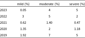
Predictors for RFI ducting have been developed utilising RFI monitoring equipment data spanning the last five years. These predictors differentiate between four levels of ducting status: none, mild, moderate, and severe. We see mild ducting 1.35% of the time, moderate ducting 4% of the time and severe ducting 3% of the time. Broken up year-on-year, the percentage of time experiencing increased RFI propagation is shown in Table 4.
Furthermore, Fig. 9 shows the location of mobile base stations that have been detected at the observatory since 2017. Base stations with larger circles indicate more numerous and the colour denotes the detected frequency. The majority of detected base stations correspond to the frequencies with increased flagging in the fixed/mobile service allocations below 800 MHz and at around 870 MHz at night shown in Fig. 8. The most frequent detections of mobile base stations come from Mullewa/Geraldton (SW) and Carnarvon (NW) directions ( $>$
5 000 detections). Detections from base stations this far (and further) away is only possible under circumstances in which there is severe ducting. Similarly, RFI from maritime vessels are detected when there is ducting. Work is ongoing within the observatory to better characterise and detect ducting both historically and operationally, including work to automatically identify it in the data and reliably predict significant ducting events in advance.
$>$
5 000 detections). Detections from base stations this far (and further) away is only possible under circumstances in which there is severe ducting. Similarly, RFI from maritime vessels are detected when there is ducting. Work is ongoing within the observatory to better characterise and detect ducting both historically and operationally, including work to automatically identify it in the data and reliably predict significant ducting events in advance.
5. Future objectives
We will continue to process, aggregate, and analyse archived 1 MHz data from other SSP. We plan to conduct regular follow-up RFI surveys and are considering a mode in which we can sample the RFI with full pointing coverage in ASKAP’s fly’s-eye mode. The first epoch of the dedicated RFI survey is currently being carried out. The survey has been designed to complement our analysis of archived data. There are two primary motivations for carrying out an RFI survey as part of the SMART project.
Firstly, frequency resolution: the data used to develop the flagstats library – and presented here within – comes primarily from archived data. The consequence of using archived data is that most of the data has a 1 MHz frequency resolution. In contrast to narrowband RFI, 1 MHz is too wide to identify interference accurately. The dedicated survey visibilities (and flags) will help plan a mitigation strategy around the RFI affecting ASKAP. Furthermore, the survey will enable us to build out the software described in the previous section and routinely process flagged data from ASKAP 18.5 kHz resolution observations, thereby better understanding the origins of RFI impinging on ASKAP science.
Second, frequency coverage, from 1 085 to 1 293 MHz and from 1 437 to 1 510 MHz of the ASKAP frequency range, is either entirely or frequently discarded after observing due to RFI. As mentioned, ASKAP SSPs generally observe in the three relatively clean bands to avoid RFI caused by satellitebased radionavigation systems (GPS, Galileo, GLONASS, and BeiDou), aeronautical radio navigation (DME and ADS-B) and satellite-based radio communication systems (Iridium, Thuraya and Globalstar) (Hotan et al. Reference Hotan2021; Indermuehle et al. Reference Indermuehle, Harvey-Smith, Wilson and Chow2017). Collecting flagged data exclusively from SSPs results in large frequency gaps where we do not understand the RFI environment or ASKAP’s default flagging behaviour (see Figs. 4 and 8).
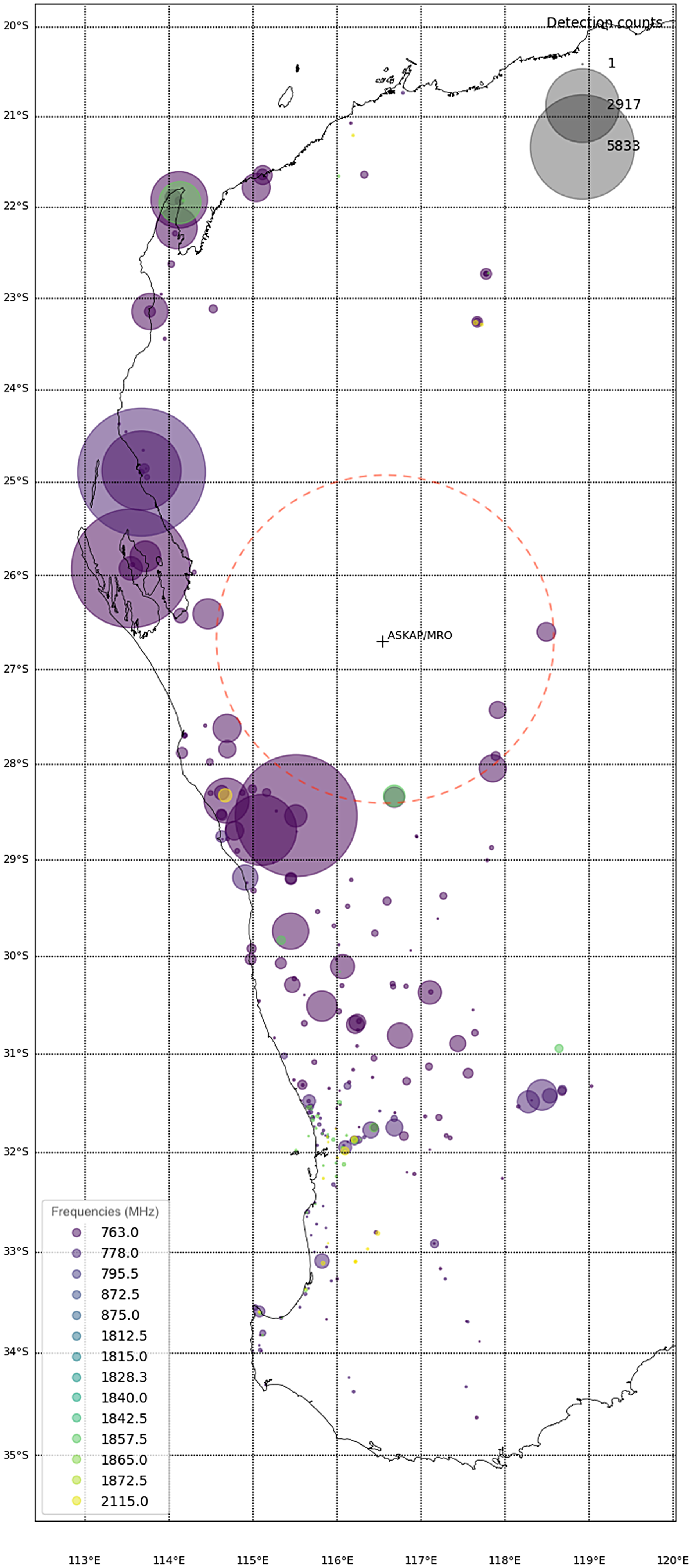
Figure 9. Map of mobile base station detections via ASKAP’s RFI monitoring equipment since 2017 showing the most frequently detected mobile base stations (the largest circles) are in the Mullewa/Geraldton (SW) or Carnarvon (NW) directions. The colour of the circles denotes the detected frequency. The map has been annotated to show the approximate area of the ARQZWA.
We are currently working on extending the software presented herein to be compatible with observations in ASKAP’s nominal full-band spectral-line resolution of 18.5 kHz (i.e. excepting zoom modes), starting with this first epoch of survey data, which will allow us to more accurately identify interferers and plan a mitigation strategy around them. We also plan to include flagged data as a function of pointing and baseline/antenna into our analysis. Full-frequency survey data will be used to calibrate and infer the suitability of RFI monitoring equipment. As part of ASKAP’s holistic RFI strategy we aim to more closely integrate the flagstats library and RFI monitoring equipment, in particular, the full-frequency telescope flagging data and high-time resolution RFI monitor data (not presented here). Finally we plan to use the RFI survey and flagged data monitoring system presented to determine and monitor the effects of RFI mitigation. This includes but is not limited to, in the short-term spatial nulling of the self-generated interferers (Lourenço & Chippendale in prep) presented in Section 4, to recover these affected frequencies.
Table 3. Percentage of scheduling blocks with excess flagging.
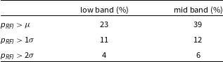
Table 4. Percentage of year experiencing increased RFI propagation.
6. Conclusion
RFI-affected data in radio astronomy is typically thrown away in a process called flagging so as not to affect scientific conclusions.The ‘Survey and Monitoring of ASKAP’s RFI environment and Trends’ project has generated an automated software processing pipeline that ingests flagged data upon completion of an observation. The software makes it easy to visualise flagging statistics due to RFI as a function of frequency and time and SSPs. Flagging statistics per observation are also stored and mapped to other sources of data to compare and analyse populations of observations in novel ways. We have presented here the implementation of this software and are currently undertaking the first in a series of regular epochs of an RFI survey with ASKAP.
We have shown the results from over 1 500 h of 1 MHz averaged data, mapped features in flagged data to their respective radio allocation to estimate the impacts on ASKAP science by other services in the radio spectrum and self-generated interferers. We have placed an upper estimate of 3% on the average data lost to RFI in the clean science bands. The (archived and processed) mid band is the least affected by flagging, while the low band is most affected by mobile telecommunication base stations.
The ongoing monitoring of all flagged data and regular full-frequency resolution RFI surveys, presented herein, are essential in improving the overall quality of science conducted with ASKAP amidst an increasingly dynamic and evolving radio spectrum.
Acknowledgements
This scientific work uses data obtained from Inyarrimanha Ilgari Bundara, the CSIRO Murchison Radio-astronomy Observatory. We acknowledge the Wajarri Yamaji People as the Traditional Owners and native title holders of the observatory site. CSIRO’s ASKAP radio telescope is part of the Australia Telescope National Facility (https://ror.org/05qajvd42). Operation of ASKAP is funded by the Australian Government with support from the National Collaborative Research Infrastructure Strategy. ASKAP uses the resources of the Pawsey Supercomputing Research Centre. Establishment of ASKAP, Inyarrimanha Ilgari Bundara, the CSIRO Murchison Radioastronomy Observatory and the Pawsey Supercomputing Research Centre are initiatives of the Australian Government, with support from the Government of Western Australia and the Science and Industry Endowment Fund.
Data availability
This paper includes archived data obtained through the CSIRO ASKAP Science Data Archive (https://data.csiro.au).


 Open access