


1. Introduction
Anthropogenic changes to ecosystem functions and derived services are essentially due to over-consumption of primary resources, human population increase and technology-driven ecosystem use intensification (Carpenter et al., Reference Carpenter, Mooney, Agard, Capistrano, DeFries, Díaz, Dietz, Duraiappah, Oteng-Yeboah, Pereira and Perrings2009; Millennium Ecosystem Assessment, 2005). The dominant economic thinking drives the development discourse (Norgaard, Reference Norgaard2010; Rees, Reference Rees2015a), and governments or national, regional and local companies do not keep systematic natural capital accounting records.
The depletion resulting from this consumption of renewable assets leads to ecosystem degradation and to the loss of their ability to provide goods and services. This is equivalent to generating negative externalities due to the consumption of ecological capital (an equivalent to depreciation or unpaid costs). Thus, the situation represents economic and political risks. Such risks are matters of national security and sovereignty, and they burden present and future generations. The Swiss Re Institute (2020) estimates that about half of the global gross domestic product (GDP) depends on high-functioning ecosystems (see also Dasgupta et al., Reference Dasgupta, Managi and Kumar2021) and Chaplin-Kramer et al. (Reference Chaplin-Kramer, Sharp, Weil, Bennet, Pascual and Daily2019) show that people’s needs for nature and the ability of nature to provide them increasingly diverge.
In society-at-large, these notions are gaining ground (Convention on Biological Diversity, 2020; Dasgupta et al., Reference Dasgupta, Managi and Kumar2021; Sustainable Development Goals, 2020; World Wildlife Fund, 2019) but remain far from being translated into coherent and convergent actionable levers of change. One such lever, namely the development of strong sustainability (Table 1) building on the evaluation of ecosystem services has been slow to gain ground.
Table 1 Glossary
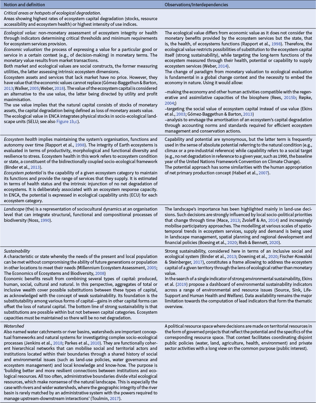
Abbreviations: ECU, ecological capability units; ENCA, ecosystem natural capital accounting.
Environmental evaluations, essential tools to socio-ecological system approaches (Bourgeron et al., Reference Bourgeron, Kliskey, Alessa, Loescher, Krauze, Virapongse and Griffith2018; Li et al., Reference Li, Dong and Liu2020; World Wildlife Fund, 2019), are being developed to assess the direct or indirect impacts of externalities on ecological systems and their productivity. These developments have contributed to the emergence of a broad range of approaches, methodologies and environmental evaluation instruments (Mazza et al., Reference Mazza, Bröckl, Ahvenharju, ten Brink and Pursula2013; Organisation for Economic Co-operation and Development, 2012; United Nations Environment Programme, 2014; Weber, Reference Weber2014; West, Reference West2015), aimed to integrate the environment and natural resources into economics-based national accounting frameworks (Caldecott et al., Reference Caldecott, Howarth and McSharry2013; Weber, Reference Weber2018). Despite such accomplishments, a recent survey concluded that ‘there is very little use of natural capital accounts for public policy decisions and, more so, in developing countries’ (Recuero Virto et al., Reference Recuero Virto, Weber and Jeantil2018). A significant reason is that political and economic decision-making and societal choices are restricted by the following limitations or contradictions in the current instruments (Argüello et al., Reference Argüello, Salles, Couvet, Smets, Weber and Negrutiu2020):
-
1. Ecosystems are often reduced to their monetary value and are aggregating distinct categories of ecosystem capital, thus hindering other possible frameworks.
-
2. Methodologies often target the ‘intensity of resource use’ and measure flow values rather than changes in stocks.
-
3. Methodologies attempting to encapsulate the GDP within more or less strict ecological limits and sustainability are heterogeneous.
-
4. Ecosystem service assessments are confronted with the challenge of the interconnected and multifunctional nature of services (e.g., avoiding double-counting or incomplete services counting or none at all).
Here, we implement a novel approach, called ecosystem natural capital accounting (ENCA), which instead considers accounts in biophysical terms.
ENCA was designed to address the notions of ecological value and ecosystem potential (Table 1) and measure degradation. The publication in 2014 of the ENCA Quick Start Package (Weber, Reference Weber2014) by the CBD Secretariat intended to support with operational methodologies the implementation by countries of the System of Economic and Environmental Accounting (SEEA) experimental Ecosystem Accounting. Considering accounts in biophysical terms, ENCA is broadly compatible with the UN Economic and Environmental Accounting System volume on Ecosystem Accounts adopted by the UN Statistical Commission in 2021 (United Nations—System of Environmental Economic Accounting, 2021). However, regarding monetary assessments, the SEEA-EA cornerstone is the valuation of the benefits provided by ecosystem services and assets, while ENCA approach to biophysical degradation leads to the calculation of unpaid restoration costs to meet the injunction of no net degradation of ecosystems. In other words, to estimate an ‘ecological value’ we depart from existing monetary valuation, which indirectly legitimise a right to exploit ecosystems, to biophysical valuation, which instead tends to consider the degradation and thus the associated biophysical debt.
The ENCA tool is based on four core accounts: land cover, water and rivers, bio-carbon and the functional services provided by the ecosystem infrastructure. This corresponds to an extension of carbon budgets (Intergovernmental Panel on Climate Change, 2006) with additional geo-physicochemical and biological parameters.
The purpose of ENCA (Figure 1) is to
-
1. describe how resource stocks and flows change over time to determine trends reflecting the real availability of each resource for use,
-
2. characterise and quantify ecosystem states with common ecological metrics to ultimately measure depletion, degradation or improvement, considering intensity of resource use in quantitative terms and diagnose ecosystem health.

Fig. 1. The ENCA accounting framework and spatially defined statistical accounting units. (a) Articulation and integration of ENCA components. The land cover and river extent account structures the three interconnected and integrated thematic accounts (bio-carbon, water and ecosystems infrastructure), while defining and implementing the statistical units for accounting. River systems are considered a particular land-cover type measured in length and run-off instead of area. Combining landscape and river systems makes it possible to blend their assessment into the infrastructure integrity account (see diagram (b) below). Thematic accounts are made using statistical and geographic data of land and river ecosystems. The protocol combines quantitative and qualitative variables. A structure common to three accounts: the landscape-scale spatial unit, the socio-ecological landscape unit (SELU) (see below)—provides internal integration. Quantitative accounts record stocks and flows for measuring the resource accessible (without depletion) and compare it to the total use. They deliver an index of intensity of use. For each account, qualitative elements help diagnose ecosystem health, as summarised in an index of landscape potential (land and river). The indices of intensity of use and health are combined to measure the mean internal ecological unit value for each component expressed in ecological capability units (ECU). Being expressed in the same unit, the resources of each thematic account can be aggregated to calculate the headline indicator of ENCA: the value of ecological capital, expressed in total ecosystem capability. The colours in the diagram indicate the degree of robustness of data sources and derived indicators. Green, very good; blue, good; orange, average; red, poor. (b) Diagram summarizing the different spatial meshes used to establish the accounts (ENCATs, UZHYD, SELU, administrative units) and illustrates the diversity of the observation levels and the corresponding sources of data mobilised during this work. The landscape-scale spatial unit, the SELU is common to the bio-carbon, water and ecosystems infrastructure accounts and provides internal integration. SELUs are statistical-geographic ecosystem units defined by a combination of dominant land-cover types (DLCT; see the map in (c) below and Supplementary Material S4a) and their respective physical properties, such as water circulation within river sub-catchments or a class of altitude. ECU values are compiled by SELU, the landscape systems where components combine and where basic ecosystem/land-cover units (agricultural land, pasture, forest, lakes and so forth) exchange and interact. (c) Map of the SELUs of the Rhône river watershed defined by the intersection of the 10 DLCT and catchments (e.g., watershed limits from BD Carthage, SANDRE, and OFEV sources). The 10 DLCTs are generated by the aggregation of 44 CLC classes. Note that natural grasslands are exclusively present in sub-alpine areas.
Ecosystem degradation is considered as the loss of ecosystem assets’ ecological value. As there is no metric for ecological value, ENCA proposes a new framework and tool to compute a unit equivalent for measuring the ecological value, that is, an aggregate summarising the various quantitative and qualitative changes recorded in the accounts, a currency of the ecosystem capital health condition. In other words, ENCA evaluates how natural assets are interconnected to respond to various pressures and reveals degradations relating to the use of the ecosystem.
The present work implements ENCA at the watershed scale and landscape resolution (Table 1). The evaluations at the river watershed scale are pertinent politically, economically, socially and ecologically because they offer systemic spatial coherence, a critical factor in managing territorial resources and ecosystem services.
The following sections report on the ENCA proof-of-concept tool applied at the Rhône river watershed scale (France) to describe the main steps of the ENCA methodology, present the results in the form of accounting tables and in cartographic form to facilitate their visualisation and analysis, supplement the conventional accounts used by private and public organisations with information allowing them to integrate in their reporting systems the accountability to ecosystem use and discuss the importance of its deployment as an aid to decision-making and societal empowerment.
2. Materials and methods
2.1 The Rhône river watershed
The report evaluates the ecosystem capital of the Rhône river watershed (Supplementary Material S1) during 2000–2012, dates corresponding to the European CORINE Land Cover Maps available at the time of the study. CORINE Land Cover (CLC) provides medium resolution maps (circa 1/100 000) updated every 6 years for the 39 European Environment Agency member and partner States (CORINE, 2017). The 2018 CLC was delivered too late for being used in this study.
The territory is a transboundary basin shared by France and Switzerland. The 97,800 km2 area encompasses several valleys and rivers in three major regions in Europe, alpine, continental and Mediterranean (Olivier et al., Reference Olivier, Carrel, Lamouroux, Dole-Olivier, Malard, Bravard, Amoros, Tockner, Uehlinger and Robinson2009). This includes five administrative regions and seven departments in the French part (more than 90% of the basin), and three cantons (Vaud, Valais and Geneva) in the Swiss portion.
We have focused our research on the French part of the watershed because the data management systems between the two countries are not fully compatible.
2.2 The ENCA methodological frame
There are four core accounts that evaluate
-
1. Land cover and use,
-
2. Water quantity and quality accounts,
-
3. Bio-carbon accounting and
-
4. Ecosystem landscape and rivers infrastructure.
The latter three represent thematic accounts framed in the land accounts and articulated by socio-ecological landscape units (SELUs) (Figure 1).
For each thematic account, the data fall into four sets of accounting tables (available at http://www.ecosystemaccounting.net/?page_id=173). A sample of a workflow is shown in Supplementary Material S2a and of an accounting table in Supplementary Material S2b.
The detailed methods can be found at https://osf.io/j93xu/ (ENCA. Proof-of-concept folder). Table 2 presents the definitions and calculation formulas of main indicators. The results are based on spatial–temporal geographic information and socio-ecological units.
Table 2 Definitions, calculation formulas, explanations on thematic indicators and considerations on data analysis
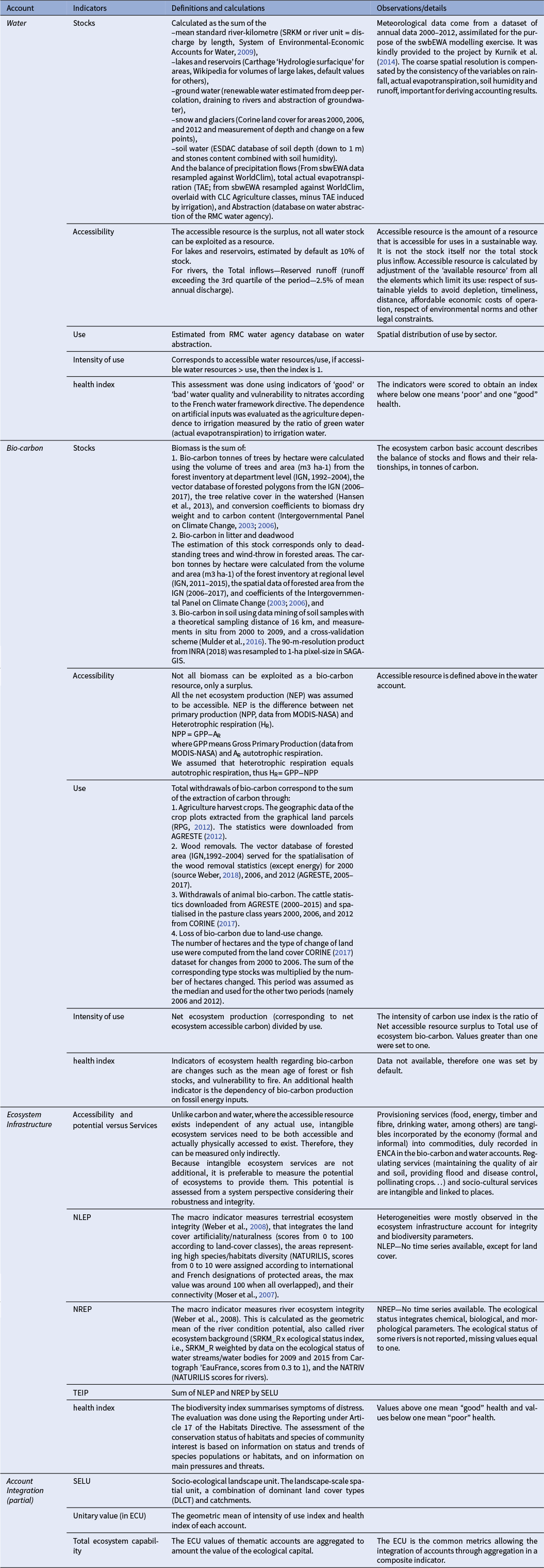
Note. Based on available data for each core account, the quantitative stocks and use balances, and resource intensity of use and health indices are calculated. Intensity of use and health indices integrate quantitative stress from resource use and qualitative diagnoses based on pollution and health assessment. They are used to estimate a composite index of ‘internal unit value’ for each core account. When no available data, a default value was taken.
Abbreviations: CLC, CORINE land cover; dominant land cover types (DLCT); ESDAC, European soil data centre; GDP, gross domestic product; GPP, gross primary production; IGN, Institut national de l’information géographique et forestière; NEP, net ecosystem production; NLEP, net landscape ecosystem potential; NPP, net primary production; NREP, net river ecosystem potential; RMC, Rhône Méditerranée Corse; SDG, sustainable development goals; SEEA-water, system of environmental-economic accounts for water; SRKM, standard river-kilometre; swbEWA, soil water balance model; TAE, total actual evapotranspiration; TEIP, total ecosystem infrastructure potential.
2.3 Land cover and river extent mapping, and conception of statistical units and account indicators
While in national accounts the statistic units are essentially legal in nature, the accounting units in ENCA are essentially geographical-spatial areas, where information is collected, and statistics are compiled from biophysical characteristics for each of the thematic accounts. In addition to SEEA’s land-cover units (i.e., ‘ecosystem accounting units’ or ‘assets’), ENCA defines ‘socio-ecological units’ which are the complexity level at which ecosystem capital accounts integration can be carried out and ecosystem degradation assessed. As for the SEEA, reporting units can be administrative or geographical divisions.
Land cover and river extent provide the frame defining the statistical units of the accounts (Figure 1b). The CLC inventory of land cover in 44 classes (1-ha pixel-size) for 2000, 2006 and 2012, and change were used to generate dominant land cover types (DLCTs). The inventory also helped to delimit the Rhône basin and hydrological sub-basins.
The combination of DLCTs and river basin boundaries defines the SELUs, the basic statistical units of ENCA (Table 2 and Figure 1c). SELUs allow for the integration of landscapes and the rivers that connect them though their run-off. The SELU has been designed to assimilate and compile input data of different sources and types (spatial resolution, geographic data, statistical data, etc.). Thus, the production of the accounts is done at the object level. We used land-cover map datasets from CORINE (2017) to analyse land cover and change.
Once the land cover and river extent frame has been defined, quantitative and qualitative data are organised for each core account.
Quantitative tables record (Table 2)
-
1. Quantities of the resource stocks and flows (basic balance),
-
2. Accessible resource surplus (computed from stocks and flows), which is the resource accessible without depletion,
-
3. Total uses by economic sectors and
-
4. Indices of the intensity of use.
Qualitative elements are used to diagnose the health state for each thematic account summarised in an index (see below and Table 2).
In general terms, the production of an integrated assessment of the ‘capability’ (or potential) of ecosystems in a standard unit, the ecological capability unit (ECU), is calculated per SELU with the available data as follows:
 $$\begin{align*}\mathrm{Total}\kern0.17em \mathrm{ecosystem}\kern0.17em \mathrm{capability}=\mathrm{UVW}+\mathrm{UVC}+\mathrm{UVEI}.\end{align*}$$
The total ecosystem capability is the sum of the ecological unitary value of water (UVW), bio-carbon (UVC) and ecological infrastructure (UVEI), expressed in ECU (Figure 1a):
These unitary values are defined by:
 $$\begin{align*}\mathrm{Unitary}\kern0.17em \mathrm{value}=\frac{\mathrm{Health}\kern0.17em \mathrm{index}+\mathrm{Intensity}\kern0.17em \mathrm{of}\;\mathrm{use}}{2}.\end{align*}$$
The health index is an assessment of the integrity of the ecosystem, based on intermediate indices for water quality, biodiversity change, and other vulnerability factors with values ranging from 0 to 1
and
 $$\begin{align*}\mathrm{Intensity}\kern0.17em \mathrm{of}\;\mathrm{use}=\frac{\mathrm{Accessible}\kern0.17em \mathrm{resources}}{\mathrm{Use}},\end{align*}$$
where values larger than 1 are set equal to 1 which means no resource depletion due to use. Values between 0 and 1 correspond to situations where use exceeds renewal.
Finally,
 $$\begin{align*}\mathrm{Accessible}\kern0.17em \mathrm{resources}=\mathrm{input}-\mathrm{output}-\mathrm{correction}\kern0.17em \mathrm{factor}.\end{align*}$$
The correction factor is needed because not all the resources are exploitable (e.g., restrictions of use in natural protected areas).
2.4 General sequence of account production
The preparatory work consisted in:
-
1. Spatio-temporal data collection (e.g., global, national, regional, municipal).
-
2. Data assimilation and integration preprocess (e.g., different tools according to the type of data, OpenOffice, Excel, QGIS, SAGA-GIS).
-
3. Spreadsheet programmes (e.g., OpenOffice or Excel).
-
4. Analysis (e.g., Postgis/PostgreSQL spatial data server and calculator Excel).
For example, the ENCA protocol includes data derived from satellite images of Earth and other maps, meteorological and hydrological data, soil maps, biodiversity monitoring data, agriculture and forestry statistics, population censuses and administrative registries. Software and geomatic treatment details are shown in Supplementary Material S3.
We then applied the following sequence.
Collecting data relating to the geographical information infrastructures necessary for the implementation of the method: delimitation of (sub)watersheds, reliefs, rivers, roads, administrative boundaries.
Collecting and organizing various sets of data (i.e., the detailed database) for accounting, namely
-
1. Socio-economic and environmental statistics,
-
2. Land cover, as land use defined by the CLC nomenclature and indexed by DLCTs (Figure 2a),
-
3. Bio-carbon (measured for total vegetation cover and soil carbon),
-
4. Water resources and
-
5. Ecological infrastructures.

Fig. 2. Land-cover accounts. (a) Land-cover main classes coverage (%) of the watershed (CORINE 2000, 2006 and 2012). The CORINE 44 land-cover types were reclassified in 10 land-cover type classes (with an additional distinction between forest categories). (b) Spatial pattern of land-cover surface change in percentage of the surface of the SELU. The shifts between land-cover categories from 2000 to 2012 (CORINE 2000–2006 and 2006–2012; see Figure 1c) represent the summary of the two time periods. (c) Absolute net changes from 2000 to 2012 resulting from the subtraction of formation (gain) minus consumption (loss) of the individual classes per period (CORINE 2000–2006 and 2006–2012) and the addition of the two periods. (d) Drivers of land-cover changes from 2000 to 2012. The drivers of change were classified according to the type of change throughout the period. According to the initial and final land-cover type, the land-cover flows are organised in a transition matrix allowing to generate all possible combinations. The analysis was performed in CLC as a postGIS object using PostgreSQL queries. The abbreviation ‘n.e.s.’ stands for not elsewhere specified.
Creation of geospatial data for each item of the thematic accounts. Data are converted to grids (rasters) of the same pixel size (1-ha pixel-size) to facilitate the calculations needed for the accounting. The processing makes it possible to aggregate the results at the level of predefined natural or artificial entities (e.g., SELUs, sub-basins, municipalities) (Figure 1b and Supplementary Material S4a).
Calculating and editing the accounting tables resulting from the extraction of information from the spatial database. Establishing an ecological balance sheet(s) in physical units.
3. Results
According to the accounting framework illustrated in Figure 1, this work reports on:
-
1. Achieving an in-depth description of the watershed biophysical resources (e.g., accessible resources description, production, supply and the intensity of their use). The framework connects to socio-economic statistics through crop harvests, timber removals, and so forth.
-
2. Establishing an ecological balance sheet in physical units and aggregating accounts in sequenced steps,
-
3. Computing synthetic indices of intensity of use and ecosystem health and integrating landscape and river systems at the SELU scale makes it possible to combine their assessment in the account of ecosystem infrastructure integrity and
-
4. Establishing the magnitude of change in the 12-year period (tables, graphs and maps) to define patterns and trends at the SELU scale. For each account, areas showing the highest rates of ecosystem capital degradation (i.e., where resources extraction surpasses renewal) are designing potential critical areas or hotspots.
3.1 Land-cover stocks and flows
Land-cover stocks correspond to the physical areas of different land-cover types. The land-cover flows account for land-cover changes, that is, conversions between land-cover categories over time grouped according to land-use drivers. They include initial land-cover losses for each land-cover type (consumption), new covers (formation) and the balance between consumption and formation. According to the initial and final land-cover type, the flows are organised in a transition matrix, making possible to generate all possible combinations. Their classification synthetically explains the kind of change between land-cover types (e.g., artificial development over agriculture). Figure 2 summarises the land accounts, focusing on subtle trends in land-cover change by SELU.
A diversity of land uses characterises the watershed, representing three dominant land-cover types: forests (more than 40%), pastures (almost 30%) and arable land (15%). The observed changes in land-use categories for the period 2000–2012 were relatively small and did not change the percentage of the main land-use categories (Figure 2a). However, cartography (Figure 2b) and data analysis (Figure 2c,d) show a sprawling effect due to the following drivers:
-
1. Land-use change, most prominent in agriculture dominated areas along the Rhône and Saône rivers, and in the northern and southern parts of the territory.
-
2. A continuous increase in artificialisation.
-
3. Forest/shrub translation flow effects due to combined losses in agricultural, pasture and forest land (e.g., changes resulting in loss of bio-carbon).
Over the 12-year period, artificialisation increased by 11%, from 4,666 to 5,163 km2, essentially to the detriment of agriculture and pastures (86%), forest (9%), other natural land cover (4%), for example, loss of fertile soils in peri-urban areas. In absolute values, agricultural and pasture land suffered a net loss of 275 km2. The degradation of forested areas (233 km2) led to an increase of transitional woodland (196 km2). Forest degradation has been predominant over restoration activities by approximately a factor of 100. Road artificialisation had impacts on ecosystem infrastructure. A decrease of Glacier area by 13% over the short period considered indicates the rate of climate change effects.
In summary, the reported land-use changes reflect the impacts of conventional agriculture practices in combination with the artificialisation of peri-urban areas and the unbalanced effects of deforestation–reforestation processes.
3.2 Ecosystem water and river accounts
The purpose of water and river accounts is to synthesise water resource measurement and its use. It explains water and river networks in the broader socio-ecological sense. An example is the interacting hydrological and user systems within the reference territory.
The definition and classification of statistical units (detailed in Table 2) comprise:
-
1. River classification (large, medium and small rivers based on their flows).
-
2. Catchment units at two scales, namely ENCA Catchment or ENCAT (the sub-basin units used for integrating land and river accounts) and elementary Hydrological Zones or UZHYD (the subdivisions of ENCATs), combined with administrative zoning.
-
3. The intersection of ENCAT boundaries of river basins with DLCTs to define SELUs for river ecosystems (Supplementary Material S4a).
A summary of the structure of ENCA water accounts is shown in Supplementary Material S4b. The main accounting categories are presented below; the definitions and calculation of main indicators being shown in Table 2.
Quantitative water accounts record exchanges between the hydrological system units, coupled with the use system of water withdrawals, consumption and returns. The results are compiled using administrative data and statistics withdrawal or estimated through population statistics multiplied by inhabitant equivalents.
River accounts closely connect to water accounts by measuring river reaches in standard river kilometres (SRKM), defined as the product of their length by the discharge (System of Environmental-Economic Accounts for Water, 2009). With SRKM, weighted rivers can therefore be aggregated.
The results on water stocks, water accessibility, water use and index of water intensity of use are shown in Figure 3. The complete water-river resource was compiled as assets by hydrological units (ENCAT and UZHYD) and the accounts reported by SELUs. The results indicate that:
-
1. The watershed is a dense, uniformly distributed hydrological system with the Alps, the Massif Central and the Cevennes serving as water ‘towers’. The precipitation regimes have been relatively stable over the studied period.
-
2. With relatively predictable water stocks, the territory has agriculture as the primary water user and shows heterogeneous and patchy patterns of change in water accessibility and intensity of use. While the average change in the watershed for water use and water intensity of use is respectively 1.5% and 0.6%, changes in the patches can be up to 40%. This is more pronounced on the Rhône river below Valence, in the drier southern part of the watershed, including the Rhône delta. Hotspots have been identified in the Dombes area (integrated agriculture and pisciculture, and industrial husbandry), south of the Léman Lake, the Chambery–Grenoble couloir, and the southern part of the watershed.

Fig. 3. Water accounts by hydrological units (UZHYD) and changes by SELU. Water balanced stocks include estimating water volume in lakes, rivers, glaciers, underwater, soil and vegetation and estimation of outflows (e.g., evaporation, run-off and transfers) and inputs (e.g., precipitation, inflows). Water accessibility reflects the balance of stock and flows, including access restrictions. Water use consists of municipal water withdrawal, agricultural and power production. The index of water intensity of use represents the surplus of water divided by use. In addition, an index has been introduced to account for groundwater stocks that are not measured per se. This approach corresponds to hydrogeology practices, such as measuring the ‘piezometric level’ and reporting, according to (Water Framework Directive) 2020. The colour code in the right panels indicates the 2000–2012 direction of change: warm colours indicate increased pressure.
Water quality and River ecological status (or potential) assessments are based on biological, physicochemical and hydro-morphological quality elements (see also Section 4). They are compiled from information reported by member States to the EU Water Framework Directive (Water Framework Directive, 2000) and the EEA technical note (European Environmental Agency, 2012).
The river ecological status decreased over the studied period (Supplementary Materials S5b and S6e,f). For example, small rivers showed degradation with rates ranging from 5 to 15%. For the main drains, the rates varied from 14 to 20%. While main drains accumulate pollutions from various origins, the network of small rivers is impacted by local pollutions (from point sources or in most cases from agriculture). Visual comparison of impacted areas and land cover clearly shows for example that vineyards north of Lyon are concerned. It contrasts with small rivers in mountain areas where rivers ecological state has improved during the same period.
In summary, the agricultural system constitutes the main source of heterogeneity in water use and the main factor of river ecological status degradation for small rivers in particular.
3.3 Ecosystem carbon accounts
So far, research on carbon accounting has explored the subject as discrete inputs and outputs (Nature Portfolio, 2018). No aggregation of carbon accounts on stocks, flows and use in biophysical values has been reported. In ENCA, bio-carbon is measured through the ecosystem’s capacity to produce biomass (crops, animal and timber biomass; converted into tons of carbon), combined with use withdrawals and losses. The accounting items, indicators and calculation formulas are given in Table 2 and Supplementary Material S2.
This ecosystem approach centres on Net Ecosystem Productivity and Net Ecosystem Carbon Balance (Schulze, Reference Schulze2006). Thus, ecosystem bio-carbon accounting categories cover a large scope of the provisioning ecosystem services and most variables used for estimating human appropriation of biomass (Haberl et al., Reference Haberl, Erb, Krausmann, Gaube, Bondeau, Plutzar, Gingrich, Lucht and Fischer-Kowalski2007).
The results are illustrated in Figure 4 and show that bio-carbon stocks are relatively stable over time (with an average of about 37 tC ha−1), with forests (trees) as the main resource (90%). There have been considerable variations in bio-carbon use and the intensity of use, showing increase of respectively 10 and 4.5% on average in the watershed, with sprawling patterns along the Saône and Rhône rivers over the studied period. The average percentage of bio-carbon use with respect to the accessible resource has been estimated at 30–40%. There has been an increase in the intensity of use over a third of the watershed (orange areas), most likely due to differences in precipitation-dependent Net Primary Production estimations.

Fig. 4. Bio-carbon accounts. Left panels—Carbon stocks (tC ha−1) by integration of data on forest (Forested surface and Timber volume from IGN data, and Tree canopy cover percentage from Hansen et al., 2013), deadwood (Forested surface and Timber volume from IGN, and Tree canopy cover percentage from Hansen et al., 2013) and soil (INRA, 2017). Carbon accessibility is calculated as the difference between net primary production (NPP) and heterotrophic respiration (data from NASA-MODIS, 2000–2014). The resulting net ecosystem production (NEP; tC ha−1) defines the accessible resource. Carbon use (tC ha−1) is calculated as the addition of agriculture harvested crops (from IGN), wood removals (from IGN) and withdrawals of animals (cattle statistics from AGRESTE and pasture class from CORINE). The index of carbon intensity of use in 2000 is calculated as NEP divided by use; values less than one indicate that the use exceeds ecosystem production, that is, degradation. The right panels show the corresponding changes (%) from 2000 to 2012. QGIS and SAGA-GIS geo-processing tools were used. The colour code in the panels indicates the 2000–2012 direction of change: warm colours indicate increased pressure.
We have identified the following hotspots:
-
1. Stocks, between Vienne and Valence agriculture couloir, where the loss of the stock ranges from 20 to 50%.
-
2. Accessibility, north and northeast areas through the Jura, Doubs and Haute–Saône within the limits of the Rhône, Saône and Loire rivers; south areas through the Drôme, Ardêche and Gard basins.
-
3. Use, through the Alps-Vercors areas mainly, with the percentage of bio-carbon use with respect to the accessible resource ranging from 32 to 42%.
-
4. Intensity of use, between Mâcon and Avignon, south of Léman lake, and Gap/Durance areas, with an index increase of 50%. The index indicates that agricultural production in some areas in the Saône river basin is not sustainable (<1, warm colours).
In summary, on a territory with large bio-carbon stocks generated by forests, the major pressure on above and below ground bio-carbon derives from agricultural appropriation of biomass. Soil bio-carbon in the watershed deserves particular focus because it remains an insufficiently characterised resource.
3.4 Ecosystem infrastructure accounts
More precisely, the ‘Ecosystem Infrastructure Functional Services Account’ relates to intangible services that can only be quantified indirectly, given people’s access to the ecosystem. It is based on quantitative, semi-quantitative and qualitative estimations of variables. They evaluate the potential access to ecosystem services and impacts on ecosystem functions through the integrity of the ecosystem infrastructure and the ecosystem health within land and river landscapes.

Fig. 5. Ecosystem infrastructure accounts (see also Supplementary Material S5). The net landscape ecosystem potential (NLEP) combines an index of greenness, an index of landscape fragmentation and an index to capture the high nature value of particular ecosystems. The net river ecosystem potential (NREP) combines the river condition potential (see Supplementary Material S5b and Supplementary Material S6f) and the index of natural conservation value for rivers. The total ecosystem infrastructure potential (TEIP) is the aggregation (sum) of NLEP and NREP by SELU. The intensity of use for NLEP, NREP and TEIP is calculated as yearly change respectively. The colour code in the right panels indicates the 2000–2012 direction of change: warm colours indicate a decreased potential, that is, an increase in pressure.
The operating frame is in Supplementary Material S5a–c and indicators definitions and calculations are shown in Table 2. The account aims at producing an assessment of net landscape ecosystem potential (NLEP) and net river ecosystem potential (NREP), based on synthetic indicators designed to characterise the integrity status of various land-cover types and river ecosystems at landscape resolution. The NLEP and NREP indices describe the evolution of such potential. SELUs aggregate the NLEP and NREP indices to compute the total ecosystem infrastructure potential (TEIP) and any changes in the respective intensity of use values.
The results are illustrated in Figure 5 and show that:
-
1. The NLEP is relatively stable over the analysed period, with a loss of potential of 2% along the Saône and Doubs rivers in the northern part, and of 3% along the Rhône and Durance rivers in the southern part of the watershed (agriculture areas mainly). We identified a hotspot on the Doubs (Basel–Montbéliard area) due to land-cover changes and the resulting fragmentation.
-
2. The NREP has a similar pattern to NLEP. Still, the changes cover larger SELUs areas than for NLEP and show either improvement (mainly in forested and pasture areas in the southern part) or degradation (mainly in agriculture dominated areas of the northern part of the watershed). It suggests that even small rivers in agricultural areas have a degraded condition (see Section 3.5), but we did not identify hotspot areas.
-
3. The TEIP reflects the combined degradation effects of land and river condition in agriculture-dominated areas (northern part more broadly, and along the Rhône valley in the southern part). The range of TEIP degradation was estimated at 0.5–30%.
In parallel, the ecosystem health analysis has been performed through the biodiversity index, and the results are illustrated in Supplementary Material S6a. We used this index to evaluate ecosystem health compared with other approaches reporting on biodiversity status on the territory (Supplementary Material S6b–d). Our results on landscape connectivity (Supplementary Material S6d, as defined in Supplementary Material S5b) allow to best capture and visualise relatively discrete fragmentation processes, suggesting that the index is a suitable proxy for biodiversity assessment. Our maps highlight a widespread and continuous degradation in species biodiversity in the French Rhône river catchment, with few exceptions in the Alps. Health index values below 1 signify degradation.
The information on land systems remains insufficient to correctly record damages of pesticides and other chemicals on ecosystem health. However, the Water Framework Directive assessment of rivers’ ecological condition (Section 2; Supplementary Material S6e and f) provided valuable information.
In summary, these observations indicate that:
-
1. The used landscape parameters provide a first hint to evaluate trends in biodiversity.
-
2. The relative coherence of ecosystem integrity and biodiversity evaluations, and the analysis at SELU scale capture the gradual degradation of increasingly fragmented ecosystems and the reduction of their potential to provide services.
3.5 First integration level of the ENCA accounts
The ENCA accounting framework has been articulated in land cover and river ecosystems. This was expected to reveal so far unexplored interdependencies between resource categories in the studied territory. The Rhône river watershed is a geographically diverse territory with important stocks of land, water, bio-carbon and a large diversity of ecosystems. Land-use patterns of change are impacting the bio-carbon balance through high levels of human biomass appropriation and contribute to the fragmentation of landscapes. Increasing rates of water intensity of use and conventional agriculture practices are the main drivers of the ecological state change affecting the rivers’ condition potential. Examples are shown in Supplementary Material S6e–g.
Taken together, the results contribute essential spatial information of ecosystem resources with quantified sprawling or patchy patterns of change at the landscape scale. This underlies the diffuse and continuous erosion of all categories of ecosystem capital and delivers early warnings of resource degradation or overuse mainly in agriculture-dominated landscapes.
These results objectify the functional interdependences among accounts. The combined impacts on carbon, water and ecosystem infrastructure resources can now be used to assess changes in the ecosystem potential. The ENCA protocol provides thus a first level of integration through intensity of use and health indices that are thematic account specific but expressed in standard (common) metrics (Figure 1a,b; Section 2.4). The aggregated indices are shown in Table 3.
Table 3 Preliminary integration of thematic accounts of the Rhône river watershed based on intermediate indices of resource intensity of use and health (see Section 2.4)

Note. When in brackets, figures are indicative or have not been calculated to avoid inconsistencies. Numbers indicate the average rate of change over 12 years. For the ecosystem infrastructure account, the intensity of use corresponds to the yearly change of TEIP, including fragmentation. The ecological health assembles chemical, biological and functional parameters. Ecological unit values are computed for each thematic account. They are derived by averaging intensity of use and ecosystem health indices (see Supplementary Material S5c for additional components of an ecosystem infrastructure).
Abbreviations: Nd, not determined; TEIP, total ecosystem infrastructure potential.
The results reflect a constant increase in the intensity of use of ecological assets, with a particular degradation of the bio-carbon balance. The average ecosystem infrastructure appeared relatively stable over the 12-year period, for two reasons. First, the network of protected areas combined with limited access conditions has contributed to maintaining the ecological potential. Second, degradation was observed when the analysis was performed by DLCTs, for wetlands in particular, along with water bodies, forests and pastures (data not shown). In general, the picture underestimates the watershed’s actual resource base condition due to limitation in available data and information. The gaps for bio-carbon health index and the ecological unit value for ecological infrastructure demonstrate this.
4. Discussion
The proof-of-concept work allowed to test and illustrate the different stages of the production chain and to identify the data required for its implementation. Based on the reported results, the question is: How does ENCA compare within the current composite and scattered methodological landscape of ecological capital evaluations?
To our best knowledge, no direct comparisons between existing methodologies have been performed so far. To achieve an in-depth understanding of their respective strengths and limitations, such comparisons would need using the same sets of data on the state and dynamics of the ecosystem capital across countries or contexts. It is likely that the required data may differently fit the specifics of such methodologies and, once performed, in context validation of the results would take more time than expected (as in this work on distinct data systems between France and Switzerland). Additional limitations need to be mentioned:
-
1. Methodological concerns, as for the ecological footprint (Blomqvist et al., Reference Blomqvist, Brook, Ellis, Kareiva, Nordhaus and Shellenberger2013).
-
2. A restricted choice of assets with as result partial accounts (Australian Bureau of Statistics, 2013; International Institute of Sustainable Development, 2018; Ouyang et al., Reference Ouyang, Song, Zheng, Polasky, Xiao, Bateman, Liu, Ruckelshaus, Shi, Xiao and Xu2020; Wigley et al., Reference Wigley, Paling, Rice, Lord and Lusardi2020), and corporate reporting on biodiversity (based on Life Cycle Assessment and Pressure-State-Response proxies; Delavaud et al., Reference Delavaud, Milleret, Wroza, Soubelet, Deligny and Silvain2021).
-
3. Indicator systems still in development (Fairbrass et al., Reference Fairbrass, Mace, Ekins and Miligan2020), and in particular those monitoring biodiversity (with some consensus on focusing assessments on ecosystem area, integrity and risk of collapse; Rowland et al., Reference Rowland, Bland, Keith, Juffe-Bignoli, Burgman, Etter, Ferrer-Paris, Miller, Skowno and Nicholson2019).
-
4. Aggregation of ecosystem service accounts in money, with preference for measuring flow values rather than changes in stocks (Economics of Land Degradation, 2015; The Economics of Ecosystems and Biodiversity, 2008).
-
5. Monetary valuation resting on micro-economic principles hardly transposable to national accounts (mainly InVest and Co$ting Nature tools to model ecosystem services provisioning for case studies; Delavaud et al., Reference Delavaud, Milleret, Wroza, Soubelet, Deligny and Silvain2021; The Economics of Ecosystems and Biodiversity, 2008; United Nations Environment Programme, 2014).
On these grounds, we argue that the best option would be the systematic assessment of the state and dynamics of the ecosystem capital covering its core components, namely land use, and the state of water/rivers, biomass and ecosystem infrastructure. This is what ENCA does, with the aim of engaging various stakeholders and the society at large in the evaluation and the stewardship of their territory. The systematic integration of the required variables in the ENCA framework, their spatial breakdown, cross-checking and update brings more than the possibility of calculating particular indicators such as total ecosystem capability and its degradation. The ENCA database is at the same time a possible source of pre-processed data for a range of other applications. As such, it would provide linkages to the variety of applications or projects. In the same vein, Fairbrass et al. (Reference Fairbrass, Mace, Ekins and Miligan2020) (see also Ekins et al., Reference Ekins, Milligan and Usubiaga-Liaño2019) propose a guide for natural capital assessment. The natural capital indicator framework organises a large number of indicators into a coherent structure of key and headline indicators based on the four-capital model of wealth creation (e.g., natural capital stocks of ecosystem and commodity assets, ecosystem flows from natural capital, human inputs and outputs in the form of benefits and residuals).
4.1 ENCA proof-of-concept: A first determinant step towards an exhaustive and integrated evaluation of ecosystem capital value
The system of ecosystem accounts approach simultaneously addresses externalities for key primary resources associated with infrastructure and ecological health, including land, water and biomass (see also Negrutiu et al., Reference Negrutiu, Frohlich and Hamant2020). By monitoring stocks and flows:
-
1. Trend values of capital stocks allow forecasting of the future potential of the stocks.
-
2. The relative value of various flows of ecosystem resources according to their use can be better understood and thus determine the extent of changes needed to address the opportunities for sustainable use.
-
3. The costs relating to the use and degradation of the ecosystems that are presently unpaid (e.g., restoration, avoidance or compensation costs) can be evaluated.
The Rhône watershed core accounts support reporting on societal targets, test territorial scenarios and catalysing action. The standard metrics and matrix—based on intensity of use and health indices for bio-carbon, water and ecosystem infrastructure—comprise an essential step forward. They enable a more systemic understanding of the territory’s strategic resources. ENCA leaves open the possibility of monetary valuation for methodological comparisons and prospective modelling.
Mapping the actual trends of resource stocks, flows and use allows the location of hotspot areas where the drivers of degradation can be identified. Such sites need verification with other sources and local actors to inform trade-offs and activate mitigation through decision-making.
Two examples illustrate the method’s strength: land-use and soils, and biodiversity and landscape.
Land cover and land-use changes constitute a fundamental issue, as seen in the overall scale of the process; it is the largest geoengineering human activity of all times (Verburg et al., Reference Verburg, Crossman, Ellis, Heinimann, Hostert, Mertz, Nagendra, Sikor, Erb, Golubiewski and Grau2015). Our analysis of land-use patterns and the state of terrestrial ecosystems in the watershed shows that it is the primary driver of ecosystem fragmentation. With a reduction in ecosystem diversity and productivity come habitat loss and degradation, biodiversity erosion and bio-carbon balance disruption (see also Barnosky et al., Reference Barnosky, Hadly, Bascompte, Berlow, Brown, Fortelius, Getz, Harte, Hastings, Marquet and Martinez2012; Steffen et al., Reference Steffen, Richardson, Rockström, Cornell, Fetzer, Bennett, Biggs, Carpenter, De Vries, De Wit and Folke2015; Urban, Reference Urban2015; Verburg et al., Reference Verburg, Crossman, Ellis, Heinimann, Hostert, Mertz, Nagendra, Sikor, Erb, Golubiewski and Grau2015).
The study targets questions such as:
-
1. How to maintain the quality and integrity of the land stock through land management (Haines-Young et al., Reference Haines-Young, Weber, Parama, Breton, Prieto and Soukup2006) to provide a better integration of soil bio-carbon and land use. There is an urgent need to arrest global agricultural land degradation, currently estimated at 67% (Prăvălie et al., Reference Prăvălie, Patriche, Borrelli, Panagos, Roșca, Dumitraşcu, Nita, Săvulescu, Birsan and Bandoc2021).
-
2. Finding solutions for the unsolved issue of a major disconnect between the financial value of land and land value according to the multifunctional capabilities of land (see also Terama et al., Reference Terama, Clarke, Rounsevell, Fronzek and Carter2019).
This is a driver of artificialisation and while ENCA has not been calibrated yet to assess all impacts of urban areas on ecological capital, urban metabolism studies (Raworth, Reference Raworth2012) can be integrated into ENCA environmental assessments.
Efforts to fix problematic issues are noticeable (Economics of Land Degradation, 2015; International Conference on Computer Design, 2017 on Land Degradation Neutrality; National Academies of Sciences, Engineering, and Medicine, 2021; Verburg et al., Reference Verburg, Crossman, Ellis, Heinimann, Hostert, Mertz, Nagendra, Sikor, Erb, Golubiewski and Grau2015). Interestingly, the EU has long-established water and air directives, but no soil directive (claimed through citizen action; European Citizens’ Initiative, 2017).
Biodiversity evaluation raises additional but no less critical concerns. There have been continuous efforts to implement a system of conventional biodiversity metrics (Biodiv2050 Outlook, 2017; Diaz et al., Reference Díaz, Zafra-Calvo, Purvis, Verburg, Obura, Leadley, Chaplin-Kramer, De Meester, Dulloo, Martín-López and Shaw2020; Pereira et al., Reference Pereira, Ferrier, Walters, Geller, Jongman, Scholes, Bruford, Brummitt, Butchart, Cardoso and Coops2013). Nonetheless, providing near real-time information for systematic and regular biodiversity assessment would be resource-intensive and have questionable relevance for decision-making (Mazor et al., Reference Mazor, Doropoulos, Schwarzmeuller, Gladish, Kumaran, Merkel, Di Marco and Gagic2018; see also Kwok et al., Reference Kwok2019; Wyborn et al., Reference Wyborn, Montana, Kalas, Davila Cisneros, Clement, Izquierdo Tort, Knowles, Louder, Balan, Chambers, Christel, Deplazes-Zemp, Forsyth, Henderson, Lim, Martinez Harms, Merçon, Nuesiri, Pereira and Pilbeam2020). To go further than the reporting to the European Habitats Directive (art. 17) (2012), a versatile biodiversity data monitoring to measure impacts systematically should take stock of the fact that changes through habitat structure remote sensing (loss, degradation), fragmentation levels and land-use change identify the primary cause of substantial changes in species abundance, distribution and interaction (Brooks et al., Reference Brooks, Mittermeier, Mittermeier, Da Fonseca, Rylands, Konstant, Flick, Pilgrim, Oldfield, Magin and Hilton-Taylor2002; Dirzo et al., Reference Dirzo, Young, Galetti, Ceballos, Isaac and Collen2014). They can be monitored simultaneously and globally (Mace et al., Reference Mace, Reyers, Alkemade, Biggs, Chapin, Cornell and Woodward2014). The ecosystem approach (Rowland et al., Reference Rowland, Bland, Keith, Juffe-Bignoli, Burgman, Etter, Ferrer-Paris, Miller, Skowno and Nicholson2019) has been designed to develop indicators on ecosystem area and integrity assessment.
This is what ENCA does. Our results show that ecosystem infrastructure and ecosystem health assessments at landscape scale proved consistent (Figure 5 and Supplementary Material S6d) compared to alternative approaches (Supplementary Material S6b and c). The ecosystem infrastructure account is an actionable proxy allowing researchers and society actors to target areas of actual or potential biodiversity erosion due to land-use change and unsustainable practices. These are areas where focusing on more detailed biodiversity assessments is required (Plumptre et al., Reference Plumptre, Baisero, Belote, Vázquez-Domínguez, Faurby, Jȩdrzejewski, Kiara, Kühl, Benítez-López, Luna-Aranguré and Voigt2021). In brief, using the landscape scale in biodiversity assessment can capture the dynamics of the process with a reasonable accuracy simultaneously and world-wide.
4.2 Data resources: The main extrinsic obstacle in deploying a complete ENCA proof-of-concept
The colour code in Figure 1a illustrates how the sequential accumulation of data limitations has been a handicap in generating aggregation indices (such as intensity of use and health indices) and working out a complete ENCA proof-of-concept. This has been the main reason for not aggregating the thematic accounts through the ecological value and capability metrics (compare Table 3). Table 4 inventories the obstacles—namely gaps and significant heterogeneity in geographically localised data production, software and processing tools—in data and information source management. It also indicates which steps in the ENCA procedure suffer most from data limitations and defines spatial entities and inconsistencies in the scales of restitution. It describes the quality of the statistics on which the measurement of the physical state of ecosystems is based.
Table 4 Obstacles (coloured cells) in the production of Rhône river watershed ENCA accounts
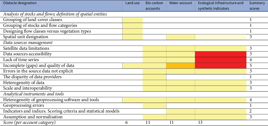
Note. Obstacles were classified into three categories and broken down by each type of account: land cover and use, bio-carbon, water and rivers, and ecological infrastructure. Pale yellow indicates the presence of obstacles in the production of the accounts with indirect impact. Yellow indicates the presence of obstacles with direct impact. Red indicates a combination of direct and indirect impacts. Orange shows that the data for the water accounts were fairly abundant and of good quality, but we encountered problems with water use, management and distribution. The final score per column ranks the accounts according to the technical difficulties encountered.
Abbreviation: ENCA, ecosystem natural capital accounting.
For example, for the bio-carbon accounts, flows data need to be completed by including carbon loss, respiration and leaching, disturbances, additional secondary stocks, inflows from other countries, and production and consumption return to the ecosystem at the required scale. For the use variables, agriculture information lacks at-scale spatial information and time series, while data on fisheries do not exist.
In short, no administrative or political authority can provide the data required to assess on a regular and consistent basis the state of the ecosystem capital in the Rhône basin territory for which they are responsible (Auvergne-Rhône Alpes, 2016). Ideally, generating annual series is an objective to reach and capture the combined result of trends and seasonal or annual fluctuations related to the meteorology (such as the Net Primary Production or evapotranspiration and rainfall).
Beyond ENCA-Rhône and despite ever-expanding satellite, sensors, geospatial data production and structuring efforts (POST, 2017), a general trend in data management is the lack of sufficiently robust, systematic and spatially explicit data collection, treatment and access systems (Moran et al., Reference Moran, Giljum, Kanemoto and Godar2020; Natural England Commissioned Report, 2020; Wilkinson et al., Reference Wilkinson, Dumontier, Aalbersberg, Appleton, Axton, Baak, Blomberg, Boiten, da Silva Santos, Bourne and Bouwman2016). Consequently, results frequently come from aggregated data or surrogate modelling and data extrapolation to remediate inaccurate data and errors. We expect the data to become findable, accessible, interoperable and reusable.
In summary, the main obstacles in data management and science concentrate on two dimensions:
-
1. Making progress towards converging concepts, definitions and methodologies in the environmental evaluation field across various player groups.
-
2. Coherent public data policies (e.g., adequately institutionalised data collection and processing) to support exhaustive, reliable and systematic evaluation of the ecosystem capital, enabling the calculation of unpaid degradation costs.
4.3 Conclusion and perspectives
Despite the above obstacles, we showed ENCA to be a methodological breakthrough, an instrument exhaustive enough to assess the ecological assets at the watershed scale and operate to monitor early warning signals of ecological capital degradation. Importantly, ENCA core accounts per se constitute already an indispensable record of data in decision-making. Displayed on an interactive dashboard, the device would indicate whether and how the degradation of resource categories spatially overlaps. The stepwise aggregation of ENCA components can provide intermediate-to-global indicators telling whether GDP growth is correlated or not to the degradation of defined resource categories of the ecosystem capital. Such relevant decision-grade information is needed in integrated resource management, landscape planning and scenario building.
At local level, ENCA can help design charters and protocols to meet project targets while helping integrate initiatives and foster partnerships and empowerment. For example, we have produced an inventory of potential partners in the territory (Parmentier et al., Reference Parmentier, Argüello, Merchez and Negrutiu2021) for networking local partnerships. The study has designed the contour of a platform for territory-actors-resources with the aim to
-
1. Facilitate arbitration and trade-offs in managing available resources,
-
2. Calibrate public markets and the conditionality of public contracts,
-
3. Helping businesses understand the state of the ecosystem capital and associated financial risks in the territories in which they operate, and
-
4. Integrate ecosystem capital accounting in local wealth assessments.
Such a co-construction effort is critical for local actors in better understanding their territory, its specifics and potential and empowers citizens to act and vote on landscape and territorial stewardship matters.
Acknowledgements
We wish to thank Charlotte Weil for her critical reading of the manuscript and productive suggestions of improvement. We are grateful to the two reviewers for their patience and precious advice in making the article accessible to all.
Financial support
This work was supported by the National Council on Science and Technology, Mexico (CONACyT) (Argüello Velazquez Jazmin Adriana, grant number 225397/410110), and the Ecole Normale Superiéure de Lyon, France: the Laboratory of Plant Reproduction and Development, the Michel Serres Institute, and the Rhône-Alpes Institute of Complex Systems.
Conflict of interest
The authors declare that they have no known competing financial interests or personal relationships that could have appeared to influence the work reported in this paper.
Authorship contributions
J.-L.W. and I.N. conceived and designed the study. J.A. and J.-L.W. conducted data gathering and performed statistical analyses. J.A. and I.N. wrote the article and J-L.W. contributed corrections and improvements.
Data availability statement
The data publicly available that support the findings of this study are available from Base de Données sur la Cartographie Thématique des Agences de l’eau (BD Carthage), Wikipedia, Coordination of information on the environment CORINE, version v.18.5, European Soil Data Centre (ESDAC), The soil water balance model (swbEWA), Base de Donnée des Limites des Systèmes Aquifères (BD LISA), Institut national de recherche en sciences et technologies pour l’environnement et l’agriculture (IRSTEA)/Office national de l’eau et des milieux aquatiques ONEMA, WorldClim, French Water Agency Rhône Méditerranée Corse (RMC), Institut national de l’information géographique et forestière (IGN), Global Forest Change 2000–2017 V1.5, Land Use/Cover Area frame statistical Survey (LUCAS), National Aeronautics and Space Administration (NASA-MODIS), Global Database of Soil Respiration Data (ORNL DAAC, NASA), Service de la statistique et de la prospective du Ministère de l’Agriculture, de l’Agroalimentaire et de la Forêt (AGRESTE), Open Street Map (OSM), Inventaire National du Patrimoine Naturel (INPN), European Environmental Agency: Habitats Directive—Art.17. Restrictions apply to the availability of resources on forestry surface and soil carbon stock, which were used under licence for this study.
Supplementary Materials
To view supplementary material for this article, please visit http://doi.org/10.1017/qpb.2022.11.


 Open access
Comments
Dear Editor-in-chief,
We submit to the QPB journal our manuscript
Ecosystem Natural Capital Accounting. Proof-of-concept - the landscape approach at watershed scale authored by Jazmin Argüello, Jean-Louis Weber, and Ioan Negrutiu.
We thank you for having invited us to contribute this manuscript to the citizen science section. This attribution makes sense because our work has benefited from a broad range of data sources and collective knowledge and expertise. This is outlined in brief below in two steps
- defining the science and society context in which our approach and work has been designed, and
- giving a brief account of the scope, results, obstacles, and perspectives of the work.
Scholars have tried to clarify the value of a healthy ecosystem given the lure of short-term profits from its incremental degradation. Still, we believe the extant body of research on this urgent topic has omitted some significant needs and concerns for natural capital evaluation.
We surveyed the field to capture current trends in environmental evaluations and classified them according to three main conceptual categories, namely (1) Pressure based indicators: reference value or limits (such as disjoint environmental indicators, ecological footprints and planetary boundaries); (2) Ecosystem services assessment and valuation; (3) Assessment of ecosystem state and degradation in a framework congruent with conventional national accounts.
There is also a lack of public data policy to support sorely needed ecosystem capital evaluation that is coherent, systematic, and exhaustive. Also, there is a need for institutionally-supported methodologies that have been peer-reviewed and are thus grounded in scientific protocols.
Thus, a scattered array of research goals and methodologies appears to have stalled a political commitment to effective ecosystem and resource stewardship, and generated confusion in the society at large as to the capacity of science to develop and recommend actionable accounting solutions that measure what counts in the general interest while moving on the road toward strong sustainability.
In this challenging context, we focused our experimental work on the assessment of ecosystem state and degradation (category number 3 above) and developed an ecosystem capital accounting tool for the Rhône river basin, a territory that possesses important stocks of bio-resources. The results are based on geographic spatio-temporal information and statistical units over a time period of 12 years. The study reveals significantly higher physical details on the dynamics of critical resources stocks and flows than previously assessed; namely land use, water and river condition, bio-carbon content of various sources of biomass, and ecosystem infrastructure. They are organized at landscape scale, a socioecological unit with convenient economic, political, and societal significance. We attempt demonstrating that the landscape unit is a suitable proxy in ecosystem capital assessment that will be able to capture the dynamics of territorial resource state with a reasonable accuracy and costs, simultaneously and world-wide.
We discuss obstacles and limitations we have been confronted with while developing the proof-of-concept and suggest improvements that will allow
- upgrading and aligning the existing instruments with the requirements of strong sustainability and the principle of "no net ecosystem degradation";
- facilitating systematic comparisons of the ecosystem capital state in space and time;
- providing a matrix for decision-making supported by a better understanding of ecosystem capital, biodiversity, and nature-society relationship;
- creating conditions to associate and involve all the actors within given territories in resource stewardship through good practice and fair reporting.
We sincerely believe our findings would appeal to the readership of QPB.
We confirm that this manuscript has not been published elsewhere in its present form and is not under consideration by another journal.