


INTRODUCTION
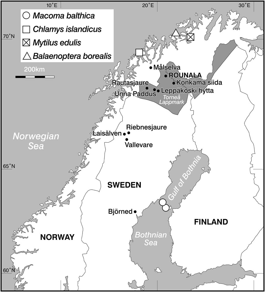
The cemetery of Rounala is associated with the historical Rounala church (Figure 1). Situated alongside one of the main trade routes between the Gulf of Bothnia and the Norwegian Sea (Hoppe Reference Hoppe1945:69), it is thought that the church at Rounala was the first church to be built in the Torne lappmark, northern Sweden. Based on historical records, Wiklund (Reference Wiklund1916:10) suggests that the church at Rounala was built in the 1500s, most likely after 1559, when a missionary was sent by King Gustav Vasa to proselytize among the Sámi in that region. The history of Sámi religious practices is complex, with periods of both Swedish and Norwegian Christianization (Aronsson Reference Aronsson2013; Kent Reference Kent2014; Rasmussen Reference Rasmussen2016). As this building was the first known church in the Torne lappmark, it could aid in our understanding of how and when Christianity was spread into this area. According to a written account, the church was abandoned in 1643, at the latest—or possibly already in 1606, as dictated by a royal decree (Wallerström Reference Wallerström2017). The church no longer stands today as it fell into disrepair after its abandonment and its material remains were sold and moved to another site during the late 18th century (Wiklund Reference Wiklund1916:12). However, during its use as a church, several people were buried at the cemetery.

Figure 1 Map of northern Fennoscandia showing the location of Rounala, the lake of Riebnesjaure, rivers of Målselva and Laisälven, the location of the reindeer samples, and the locations of the marine species used to calculate marine ΔR values. The shaded area denotes Torne lappmark (see main text).
During the excavation in 1915 by Eskil Olsson, the remains of 23 distinct humans were identified (Wiklund Reference Wiklund1916:17–19). According to Manker (1961:96), the burial styles are somewhat diverse, probably reflecting a mix of Sámi and Christian traditions, as recently discussed by historian Siv Rasmussen (Reference Rasmussen2016). The possibility that the graveyard was in use prior to the founding of the church must not be disregarded. Here we aim to date the burial events of the interred individuals so as to understand the relationship between the graveyard and the church; did the burials begin before the church’s construction?
A careful calibration of the individuals’ radiocarbon (14C) dates will be necessary to establish the time of burial. This calibration must be made with regard to reservoir effects potentially influencing these samples. Marine and freshwater reservoir effects occur due to the accumulation of 14C depleted carbon (Ascough et al. Reference Ascough, Cook and Dugmore2005; Philippsen Reference Philippsen2013). Different environmental sources of radiocarbon, 14C reservoirs or pools depleted in 14C, yield different average 12C/14C ratios. This being the case, modern samples from these reservoirs can be measured as having apparently old 14C dates. These 14C reservoir effects can alter a sample’s apparent age by hundreds or even thousands of years. Stable isotope analysis, used to reconstruct diets, can be used to quantify the dietary input from different reservoirs, thereby enabling the estimation of the true age of an individual.
The effect of multiple reservoir effects from different dietary sources on 14C dating has been previously studied by, e.g. Ascough et al. (2007, Reference Ascough, Church, Cook, Dunbar, Gestsdóttir, McGovern, Dugmore, Friðriksson and Edwards2012) and Sayle et al. (2014, Reference Sayle, Hamilton, Gestsdóttir and Cook2016). To address this problem, a series of steps must be taken to accurately date the human remains. Firstly, a multi-isotopic model will be used to help reconstruct the diet of these individuals. Secondly, the presence of any freshwater reservoir effects must be investigated. Thirdly, appropriate ΔR values will be defined for each individual. Finally, an OxCal model, which considers all available reservoir effects and dietary inputs, will be used to calibrate the 14C dates of these individuals.
Regarding the procurement of these dietary resources, Sámi economies in northern Scandinavia were quite diverse. Sámi cultures have often been subdivided in order to account for these economic differences. The Sea Sámi lived traditionally by combining fishing and small-scale animal husbandry. The term Reindeer Sámi, or Mountain Sámi, describes the nomadic Sámi peoples living as reindeer herders. Forest Sámi traditionally lived by combining fishing in inland rivers and lakes alongside small-scale reindeer-herding (Vorren and Manker Reference Vorren and Manker1976:106, 118–119). This investigation into the diets of the Rounala individuals falls into ongoing research and discussion of Sámi subsistence and settlement patterns. A historical map shows that many Forest Sámi settlements were placed close to rivers and lakes (Norstedt and Östlund Reference Norstedt and Östlund2016). This settlement pattern is consistent with ethnographic descriptions of groups with a fish-centered subsistence pattern but perhaps not with a reindeer-centered one (Norstedt and Östlund Reference Norstedt and Östlund2016). It has also been proposed that fish (Norstedt et al. Reference Norstedt, Axelsson and Östlund2014) were more important than has previously been assumed.
MATERIALS
In total, 19 human skeletal samples from Rounala were anlaysed. Although 23 distinct human individuals were identified during the original excavations, only 21 of the crania were in a condition suitable for recovery. Today only 17 of these 21 crania could be located. A further two human humerus samples from Rounala were sampled for analysis. In addition, 22 faunal samples were analyzed: eight modern fish and 14 reindeer. Three Atlantic salmon were caught from the estuary of Målselva (northern Norway), a 140-km-long river emptying into the Malangen fjord in the Norwegian Sea. Samples of the salmon muscle and bone were taken for stable isotope analysis and 14C dating. Five specimens of freshwater fish were caught from freshwater bodies in northern Sweden; these included four Arctic char and one brown trout. Archaeological and historical samples from 14 reindeer were sampled from a number of sites in northern Sweden (Figure 1). Data from these samples were considered alongside previously published data, including 54 Atlantic cod and 18 Baltic seals, used to infer Baltic fish values.
METHODS
Human and Reindeer Bone Collagen
To reconstruct the diet of the humans interred at Rounala, stable isotope analysis was performed on bone collagen extracted from human bones, as well as from faunal bones representing animals that were potentially consumed by the human individuals. Samples of human and reindeer bone powder were obtained using a dentist’s drill. Surface layers were discarded to avoid contamination. Bone collagen was subsequently extracted by the method of Brown et al. (1988), a modification of the Longin method (1971). This included an ultrafiltration step to remove the <30 kDa fraction which potentially contains contaminants of low molecular weight. All sampling and extraction were performed at Stockholm University Archaeological Research Laboratory while subsequent EA-IRMS analysis took place at Stockholm University Stable Isotope Laboratory (SIL), Dept. of Geological Sciences, unless otherwise stated. Bone collagen was weighed into tin capsules (ca. 0.5 mg for carbon and nitrogen isotope analysis and ca. 2–5 mg for sulfur isotope analysis) for combustion in a Carlo Erba NC2500 elemental analyzer connected to a continuous flow isotope ratio mass spectrometer—a Finnigan MAT Delta+ for δ13C and δ15N, and a DeltaV Advantage for δ34S measurements. The precision of the measurements was ±0.15‰ or better for both δ13C and δ15N ratios, and ±0.2‰ or better for δ34S measurements.
Fish Muscle and Bone Collagen
Arctic char and brown trout bone samples were boiled, after which bone was subsequently mechanically defleshed. Bone collagen was extracted following the same protocol as outlined above with the addition of a lipid removal step after demineralization. A 2:1 dichloromethane:methanol solution was added, after which samples were shaken for two hours, then rinsed with deionized water in excess and subsequently dried in a desiccator overnight.
The bone and flesh of the Atlantic salmon were mechanically separated. Both muscle and bone samples were subject to lipid removal procedures as above. Samples were then placed in a heating block at 70°C until dry. Collagen was extracted from these salmon samples using the following method: Bone samples were placed in 8 mL of 0.6M HCl at 4ºC until demineralized. The samples were rinsed with deionized water and left to gelatinise in 4 mL of HCl (pH3) in a heating block at 80ºC until the collagen had fully dissolved (Longin Reference Longin1971; Richards and Hedges Reference Richards and Hedges1999; Colonese et al. Reference Colonese, Thomas, Lucquin, Firth, Charlton, Robson, Alexander and Craig2015). Ultrafilters were rinsed with 0.1M NaOH and centrifuged at 850 g for 8 min to remove any contaminants. This process was repeated three times with deionized water. The bone samples were centrifuged down to 0.5 mL and freeze-dried. The lipid-removed muscle samples were freeze-dried and ground down to a powder.
Radiocarbon Dating
AMS 14C dating was performed on bone collagen from the 19 Rounala human individuals, the modern fish samples, consisting of one Arctic char, one brown trout and three salmon, as well as muscle collagen extracted from the three salmon samples. 14C dating was performed at the AMS facility at the Dept. of Physics and Astronomy at Uppsala University (a few previous dates of human bone had been made at the Radiocarbon Dating Laboratory at Lund University; see Appendix 1).
RESULTS
All faunal and human samples, except the modern salmon, complied with established collagen quality criteria with regard to yield, carbon and nitrogen concentrations and atomic C:N ratio, as well as sulphur concentration, atomic C:S and N:S ratios (DeNiro Reference DeNiro1985; Ambrose Reference Ambrose1990; Nehlich and Richards Reference Nehlich and Richards2009) (due to machine failure, one of the fish, REB 1, did not generate any carbon and nitrogen data). Some of the modern salmon samples have C:N ratios slightly out of range and very high sulphur concentrations, the latter affecting the C:S and N:S ratios. Given that these samples are modern, and that C:S and N:S ratios are consistent both between muscle and bone collagen from the same individual, and also between individuals, these samples have been included in subsequent analysis.
Stable isotopic results are summarized in Figures 2–3 and Table 4 (detailed data in Appendix 2). The only terrestrial animal in this study, reindeer, display δ13C values ranging from −21.7‰ to −18.5‰ and δ15N values between 2.0‰ and 5.9‰, consistent with previously analyzed reindeer (Iacumin et al. Reference Iacumin, Nikolaev and Ramigni2000; Salmi et al. Reference Salmi, Äikäs, Fjellström and Spangen2015). The δ34S values range from 7.9‰ to 12.8‰, reflecting the large geographical area the reindeer derive from. The freshwater fish display δ13C values ranging from −22.6‰ to −19.0‰, δ15N values between 5.8‰ and 7‰ and δ34S values range from 8.2‰ to 9.2‰. The Atlantic salmon bone samples have δ13C values ranging from −19.5‰ to −17.6‰, δ15N values between 10.1‰ and 12.4‰ and δ34S values between 17.4‰ and 18.3‰.

Figure 2 Graph displaying δ13C and δ15N values for the Rounala humans and relevant food groups (mean ±1 standard deviation). The δ13C values for modern samples have been corrected for the Suess effect by +1.5‰. Reindeer n=14 (this study), freshwater fish n=5 (this study), Baltic fish n=18 (Enhus et al. Reference Enhus, Boalt and Bignert2011), Atlantic salmon n=3 (this study), Atlantic cod n=51 (Barrett et al. Reference Barrett, Orton, Johnstone, Harland, Van Neer, Ervynck, Roberts, Locker, Amundsen, Enghoff, Hamilton-Dyer, Heinrich, Hufthammer, Jones, Jonsson, Makowiecki, Pope, O’Connell, de Roo and Richards2011; Nehlich et al. Reference Nehlich, Barrett and Richards2013). See Discussion section for Baltic fish values.

Figure 3 Graph displaying δ13C and δ34S values for the Rounala humans and relevant food groups (mean ±1 standard deviation). The δ13C values for modern samples have been corrected for the Suess effect by +1.5‰. Reindeer n=14 (this study), freshwater fish n=5 (this study), Baltic fish n=18 (Linderholm et al. Reference Linderholm, Andersson, Mörth, Grundberg, Hårding and Lidén2008; Enhus et al. Reference Enhus, Boalt and Bignert2011), Atlantic salmon n=3 (this study), Atlantic cod n=51 (Barrett et al. 2011; Nehlich et al. Reference Nehlich, Barrett and Richards2013). See Discussion section for Baltic fish values.
Stable isotope values vary along food chains. Typically, there is a large stepwise trophic shift of between +3 and 5‰ in δ15N from prey to consumer (Minagawa and Wada Reference Minagawa and Wada1984; Bocherens and Drucker Reference Bocherens and Drucker2003). A smaller trophic-level effect of about between +1 and 2‰ is observed for δ13C values between prey and consumer (DeNiro and Epstein Reference DeNiro and Epstein1978). Trophic level shifts in δ34S values between animals and their diet are 0±1‰ (Barnes and Jennings Reference Barnes and Jennings2007; Kaufman and Michener Reference Kaufman and Michener2007).
The isotopic values for the humans range between −18.5‰ and −17.2‰ (δ13C), 10.2‰ and 14.8‰ (δ15N) and 7.7‰ and 12‰ (δ34S), showing a wide variation. The δ13C and δ15N values are particularly elevated relative to the reindeer, indicating that reindeer did not constitute a major dietary source. Furthermore, the humans have δ15N values similar to the marine fish groups, but considerably lower δ13C values, indicating some marine input, but no linear mixing between solely two major food groups. FRUITS (Food Reconstruction Using Isotopic Transferred Signals), a Bayesian computer model for diet reconstruction, will help estimate the contributions of these marine groups (Fernandes et al. Reference Fernandes, Millard, Brabec, Nadeau and Grootes2014).
The results of the 14C dating and stable isotope analysis applied to the human samples are summarized in Table 1. Duplicate 14C measurements were made for humans 6, 10 and 12, due to their larger uncertainties; their 14C ages were calculated using R_Combine in OxCal v.4.3, (Bronk Ramsey Reference Bronk Ramsey2009; see Appendix 1 for sample details).
Table 1 Stable isotopic ratios and 14C ages of Rounala human samples (see Appendix 1 for details).

Table 2 displays stable isotopic and calibrated 14C data for the fish sampled, demonstrating that all 14C dates are consistent with modern samples—both the freshwater species and the Atlantic salmon. Calibrated dates were calculated from 14C pMC values using the 14CALIBomb software (Reimer and Reimer Reference Reimer and Reimer2004). At 95.4% probability, the collagen samples are clearly modern.
Table 2 Stable isotope ratios and calibrated 14C ages for the fish samples.

Salmon are a migratory fish species, spending some time in marine systems and traveling upriver to spawn. The amount of time these salmon had spent in the river was not known. Due to the difference in turnover rates between bone and muscle tissue, the effect of migration on the 14C values of these fish could be investigated. There was, however, no reservoir effect noticed in any of the tissues. This was surprising considering the potential migration of these species into marine waters, where there is a known reservoir effect. There appears to be some difference in terms of the δ34S values between salmon tissues, which could be explained by differing turnover rates. Salmon muscle δ13C values were depleted relative to bone collagen whereas δ15N muscle values were enriched. δ34S values were more variable between tissues. Arctic char and brown trout are landlocked freshwater species in this area, and treated as their own group in the FRUITS modeling. The salmon samples also form their own group.
DISCUSSION
Defining Marine ΔR Values
ΔR values for both the North Norwegian Sea and the Bothnian Sea were calculated. ΔR values represent regional offsets from the global average surface water marine reservoir effect, the ΔR of this average being ΔR=0 (Russell et al. Reference Russell, Cook, Ascough, Scott and Dugmore2011). Table 3 presents the marine samples used to calculate the ΔR values for the North Norwegian Sea and the Bothnian Sea. Note the low ΔR value that is calculated for the Bothnian Sea, which is due to the number of freshwater rivers emptying into the north of the Baltic Sea. In fact, the ΔR value for the northernmost part of the Baltic, the Gulf of Bothnia, is likely to be even lower, considering the correlation between salinity and reservoir age (Lougheed et al. Reference Lougheed, Filipsson and Snowball2013), but there is currently no data available on this.
Table 3 Summary of marine samples and ΔR values for the Bothnian Sea and North Norwegian Sea. Weighted mean ΔR values and uncertainties calculated using the Calib Marine Reservoir Correction tool.

Dietary Modeling
To investigate the diet of the Rounala individuals, FRUITS 3.0 modeling software (Fernandes et al. Reference Fernandes, Millard, Brabec, Nadeau and Grootes2014) was employed. This required the isotopic characterization of various food groups which were likely to have contributed to the diet of the Rounala individuals. From historical sources, it is known that fish were an important dietary input, also for the people in Rounala (Nickul Reference Nickul1977:3, 10, 15, 32; Ruong Reference Ruong1982:22–26; Fjellström Reference Fjellström1985:22–44; Korpijaakko-Labba Reference Korpijaakko-Labba1994:81–86, 91–93; Bergman and Ramqvist Reference Bergman and Ramqvist2017). In northern Scandinavia there are many lakes and large rivers from which freshwater fish would have been caught. Because Rounala is positioned between the North Norwegian Sea (100 km) and the north Baltic Sea (330 km), fish from both marine water bodies also need to be considered as a food source. Reindeer too were considered as a potentially important dietary resource. Each dietary group was defined by their δ13C, δ15N, and δ34S values, respectively, and the proportions of three different aquatic resources were calculated by this model (Table 4, Appendix 3). The δ13C measurements for modern collagen samples were adjusted for the Suess effect by adding 1.5‰ (Keeling Reference Keeling1979). FRUITS models were both non-routed and concentration independent.
Table 4 Summary of average δ13C, δ15N, and δ34S values with standard deviations of faunal groups, see Appendix 3 for individual samples (Barrett et al. Reference Barrett, Orton, Johnstone, Harland, Van Neer, Ervynck, Roberts, Locker, Amundsen, Enghoff, Hamilton-Dyer, Heinrich, Hufthammer, Jones, Jonsson, Makowiecki, Pope, O’Connell, de Roo and Richards2011; Nehlich et al. Reference Nehlich, Barrett and Richards2013). Baltic fish values calculated from Enhus et al. (Reference Enhus, Boalt and Bignert2011) and Linderholm et al. (Reference Linderholm, Andersson, Mörth, Grundberg, Hårding and Lidén2008), see main text.

Few studies using stable isotope data from the North Baltic are published. In order to isotopically define the Baltic fish food group, published seal data was considered. Enhus et al. (Reference Enhus, Boalt and Bignert2011) measured the δ13C and δ15N values of bone collagen from one harbour seal, eight grey seal and eight ringed seal. In total, these 17 individual seals from the North Baltic yielded δ13C and δ15N values of −18.1±1.6 and 15.6±1.7 respectively. These values were adjusted to represent the Baltic fish consumed by the seals, by subtracting 1.5‰ from the δ13C value and 4‰ from the δ15N value to correct for the trophic-level shift (the application of different fractionation offsets between 3‰ and 6‰ for δ15N made no substantial difference). For each Baltic fish isotopic value, the root sum squared of the associated fractionation offsets and the standard deviation of each isotopic value was taken to be the uncertainty. A δ34S value of 12.6‰ was measured from a seal sample that was recovered from Björned, Torsåker parish, Ångermanland (Linderholm et al. Reference Linderholm, Andersson, Mörth, Grundberg, Hårding and Lidén2008), from which we subtracted 0.5‰, and assumed a standard deviation to equal 1‰. These uncertainties can be seen in Table 4.
Isotopic values for relevant dietary groups (Table 4) were placed into FRUITS models (Fernandes et al. Reference Fernandes, Millard, Brabec, Nadeau and Grootes2014). The models assumed fractionation offsets of +1.5±0.5‰ for δ13C values, +4±1‰ for δ15N values and +0.5±0.5‰ for δ34S values between the collagen of the food source and consumer. For each human sample, uncertainties of 0.15‰ were applied to carbon and nitrogen measurements and 0.2‰ for sulfur measurements, in line with instrumentation error. No dietary priors were applied to the models. The purpose of these models were to estimate the dietary input of aquatic sources which carry with them a 14C reservoir effect.
OxCal Modeling
Two OxCal 4.3 models (Bronk Ramsey Reference Bronk Ramsey2009) were prepared as part of the recalibration of the Rounala individuals, one “mixed marine-reservoirs” model and one “Baltic reservoir” model. Based on the 14C dates of modern freshwater fish and salmon, no reservoir effect from freshwater fish or from Atlantic salmon (or from reindeer) is considered. Both OxCal models required separate dietary analysis to assess marine protein contributions.
The first OxCal model, “mixed marine-reservoirs,” assumed dietary inputs from reindeer, freshwater, Atlantic cod and Baltic fish food groups. Because each human was found to consume different amounts of Baltic and Atlantic resources, respectively, and because samples from these two environments carry different ΔR values, each human sample was assigned a unique ΔR value. These unique ΔR values were averages of the Baltic and Atlantic ΔR values, weighted according to the mean Atlantic and Baltic dietary inputs of each individual, as calculated by the FRUITS model. The errors associated with the Baltic and Atlantic ΔR values were propagated to 36.2, and this value was set as the uncertainty for each consumer’s unique ΔR values. The data was calibrated against the IntCal13 and Marine13 curves (Reimer et al. Reference Reimer, Bard, Bayliss, Warren Beck, Blackwell, Bronk Ramsey, Buck, Cheng, Lawrence Edwards, Friedrich, Grootes, Guilderson, Haflidason, Hajdas, Hatté, Heaton, Hoffmann, Hogg, Hughen, Felix Kaiser, Kromer, Manning, Niu, Reimer, Richards, Marian Scott, Southon, Staff, Turney and van der Plicht2013). The total marine dietary input for each individual was calculated by combining their Baltic and Atlantic mean marine input estimates. The total marine dietary input uncertainty was taken to be the root sum squared of the Baltic and Atlantic mean estimates. The data used to construct this model have been summarized in Table 5.
Table 5 Summary for information entered into the “mixed marine-reservoirs” OxCal model.
The second OxCal model, “Baltic reservoir,” considered some historical information concerning the dietary practices of these individuals. On historical grounds, it is known that salmon were particularly important to the Sámi living in the north of Scandinavia; salmon fishing was practiced widely along several rivers (Kent Reference Kent2014:240–246). For the people in Rounala, the river of Storfjordselva, characterized as a good salmon carrying river, was particularly important (Korpijaakko-Labba Reference Korpijaakko-Labba1994:91f; Guttormsen Reference Guttormsen2005:431, 417). As such, reindeer, freshwater fish, Baltic fish, and Atlantic salmon were considered as part of a FRUITS model, whereas Atlantic cod was excluded. Because no reservoir effect could be measured in the salmon sampled in this study, this OxCal model considered only Baltic ΔR values and Baltic marine dietary estimates and calibrated samples against IntCal13 and Marine13 curves (Reimer et al. Reference Reimer, Bard, Bayliss, Warren Beck, Blackwell, Bronk Ramsey, Buck, Cheng, Lawrence Edwards, Friedrich, Grootes, Guilderson, Haflidason, Hajdas, Hatté, Heaton, Hoffmann, Hogg, Hughen, Felix Kaiser, Kromer, Manning, Niu, Reimer, Richards, Marian Scott, Southon, Staff, Turney and van der Plicht2013) (Table 6). This assumes that the only reservoir effect acting on the Rounala consumers would come from the Baltic.
Table 6 Summary for information entered into the “Baltic reservoir” OxCal model, assuming a ΔR value of −189±4.
Some prior information concerning the church and the graveyard’s use was included in both OxCal models. It is known on historical grounds that the church was used less frequently by 1643 (Lidén et al. in press). The church building itself was sold in 1796 and dismantled (Wiklund Reference Wiklund1916:12). Based on this, a maximum calendar date for the buried individuals of 1800 AD was used, which gives some room for error. The model would not accept age estimates for samples which fell after this date. No earliest date was set.
The probability distributions of the Rounala consumers as calculated by both OxCal models are displayed in Figure 4. The distribution plots represent a range of possible ages. The range takes into account any uncertainties included in the OxCal model. Here, uncertainties associated with ΔR values, marine dietary contribution and calibration curves have led to some broad probability distributions, even at 68.2% probability. The differences between the two OxCal models are minor. In general, the model which assumed only salmon constituted the Atlantic dietary contribution (the “Baltic reservoir” model), yielded slightly older mean estimates. The two models, however, share a similar pattern. The amount of Atlantic salmon consumed by the Rounala individuals, relative to Atlantic cod consumed, cannot be estimated with any reasonable certainty. Given the overlap of the two calibration models, this should not affect the calibration of their 14C dates. Dashed lines at 1559 AD and 1800 AD represent the earliest possible founding of the church and the latest possible abandonment of the church, respectively, based on historical records. The distribution plots, relative to the estimates of the church’s founding, indicate that it is likely that many individuals (to varying degrees of certainty) were interred in the cemetery before 1559 AD. It must be noted, however, that the events being dated are the formations of the bone tissues sampled rather than the date of death. In some individuals, part of the tissue may have formed up to 20 years prior to their burial, depending on their age at death. Given this, the date of some of the individual’s burial events may have been slightly overestimated (their true burial dates being more recent than estimated). This is likely to be the case for all adult individuals (excluding the subadult individuals 16, 18, 20, and 21). From the available evidence presented here and considering all uncertainties, however, the site of the cemetery was most likely in use for a time prior to the church’s founding, as well as after its alleged abandonment. Calibrated without prior date constraints, samples 16 and 21 yield later dates, closer to present, especially for the mixed marine model. Knowing their archaeological contexts, this demonstrates the importance of the inclusion of the date constraint.

Figure 4 OxCal plot displaying the 68.2% and 95.4% probability distributions and mean age estimates (marked with a circle) of both models for Rounala samples. Dashed lines at 1559 AD and 1800 AD represent the earliest possible founding and the latest possible abandonment of the church, respectively, based on historical records. The model would not accept age estimates for samples which fell after 1800 (see main text).
CONCLUSION
Despite historical records on the building and abandonment of the church at Rounala, the relationship between the cemetery and the church had yet to be investigated fully. The timing of the burial of these individuals is important for wider discussions concerning the religious practices of these individuals as well as the Christianization of the Sámi in this region. It was demonstrated, by measuring the 14C values of modern freshwater fish from the region, that there does not appear to be a freshwater reservoir effect in the bodies of water investigated; this was an important point to illustrate. From the available evidence presented here and considering all uncertainties, the site of the cemetery was most likely in use for a time prior to the church’s earliest possible founding, possibly as early as the 14th century, but also after its alleged abandonment. The majority of the sampled individuals, however, appear to have been buried throughout the graveyard’s use as a church site.
ACKNOWLEDGMENTS
This project has received funding from the European Union’s EU Framework Programme for Research and Innovation Horizon 2020 under Marie Curie Actions Grant Agreement No. 676154. This research has benefited from several useful discussions with Prof. Peter Jordan (The Arctic Centre, University of Groningen). Thanks go to Geoffrey Metz at the Museum Gustavianum in Uppsala, Leena Drenzel at the Swedish History Museum in Stockholm, Kjell-Åke Aronsson at Ájtte – the Swedish Mountain and Sami Museum in Jokkmokk, to the Nordic Museum in Stockholm, for access to the skeletal material, Anna Kjellström for making the osteological analysis of the human material, to Charlotte Damm for the Atlantic salmon, and to Heike Siegmund at SIL for running the EA-IRMS. Some of the stable isotope data formed part of MF’s master’s thesis (Fjellström Reference Fjellström2011).
SUPPLEMENTARY MATERIAL
To view supplementary material for this article, please visit https://doi.org/10.1017/RDC.2018.78
Appendix 1. Lab codes and 14C ages reported for Rounala human samples.

Appendix 2. The δ13C, δ15N and δ34S values and collagen quality indicators for the Rounala humans and analyzed reindeer and fish. Samples and δ13C values marked with an (*) have been adjusted for the Suess effect (δ13C +1.5‰).

Appendix 3. The δ13C, δ15N and δ34S values of faunal samples used for FRUITS modeling. Samples marked with an (*) have δ13C values adjusted for the Suess effect.

Appendix 4. OxCal model code
Plot()
{
Curve(“IntCal13”,“IntCal13.14c”);
Curve(“Marine13”,“Marine13.14c”);
Delta_R(“LocalMarine”,-115.5,36.2);
Mix_Curve(“Mixed”,“IntCal13”,“LocalMarine”,41.8,19.5);
R_Date(“Mixed Marine 6”, 669, 65) & Date(U(0,1800));
Curve(“IntCal13”,“IntCal13.14c”);
Curve(“Marine13”,“Marine13.14c”);
Delta_R(“LocalMarine”,-189,4);
Mix_Curve(“Mixed”,“IntCal13”,“LocalMarine”,28.7,16.1);
R_Date(“Baltic Marine 6”, 670, 65)& Date(U(0,1800));
Curve(“IntCal13”,“IntCal13.14c”);
Curve(“Marine13”,“Marine13.14c”);
Delta_R(“LocalMarine”,-126.0,36.2);
Mix_Curve(“Mixed”,“IntCal13”,“LocalMarine”,22.0,14.0);
R_Date(“Mixed Marine L17b”, 550, 32) & Date(U(0,1800));
Curve(“IntCal13”,“IntCal13.14c”);
Curve(“Marine13”,“Marine13.14c”);
Delta_R(“LocalMarine”,-189,4);
Mix_Curve(“Mixed”,“IntCal13”,“LocalMarine”,14.5,11.3);
R_Date(“Baltic Marine L17b”, 550, 32) & Date(U(0,1800));
Curve(“IntCal13”,“IntCal13.14c”);
Curve(“Marine13”,“Marine13.14c”);
Delta_R(“LocalMarine”,-107.8,36.2);
Mix_Curve(“Mixed”,“IntCal13”,“LocalMarine”,32.7,15.1);
R_Date(“Mixed Marine 1”, 580,85) & Date(U(0,1800));
Curve(“IntCal13”,“IntCal13.14c”);
Curve(“Marine13”,“Marine13.14c”);
Delta_R(“LocalMarine”,-189,4);
Mix_Curve(“Mixed”,“IntCal13”,“LocalMarine”,22.2,14.3);
R_Date(“Baltic Marine 1”, 580,85)& Date(U(0,1800));
Curve(“IntCal13”,“IntCal13.14c”);
Curve(“Marine13”,“Marine13.14c”);
Delta_R(“LocalMarine”,-136.8,36.2);
Mix_Curve(“Mixed”,“IntCal13”,“LocalMarine”,19.4,12.6);
R_Date(“Mixed Marine 8”, 527, 30) & Date(U(0,1800));
Curve(“IntCal13”,“IntCal13.14c”);
Curve(“Marine13”,“Marine13.14c”);
Delta_R(“LocalMarine”,-189,4);
Mix_Curve(“Mixed”,“IntCal13”,“LocalMarine”,16.1,14.7);
R_Date(“Baltic Marine 8”, 527, 30)& Date(U(0,1800));
Curve(“IntCal13”,“IntCal13.14c”);
Curve(“Marine13”,“Marine13.14c”);
Delta_R(“LocalMarine”,-118.4,36.2);
Mix_Curve(“Mixed”,“IntCal13”,“LocalMarine”,30.0,15.8);
R_Date(“Mixed Marine 13”, 513, 30) & Date(U(0,1800));
Curve(“IntCal13”,“IntCal13.14c”);
Curve(“Marine13”,“Marine13.14c”);
Delta_R(“LocalMarine”,-189,4);
Mix_Curve(“Mixed”,“IntCal13”,“LocalMarine”,25.1,15.7);
R_Date(“Baltic Marine 13”, 513, 30)& Date(U(0,1800));
Curve(“IntCal13”,“IntCal13.14c”);
Curve(“Marine13”,“Marine13.14c”);
Delta_R(“LocalMarine”,-150.4,36.2);
Mix_Curve(“Mixed”,“IntCal13”,“LocalMarine”,41.7,19.5);
R_Date(“Mixed Marine 20”, 552, 30) & Date(U(0,1800));
Curve(“IntCal13”,“IntCal13.14c”);
Curve(“Marine13”,“Marine13.14c”);
Delta_R(“LocalMarine”,-189,4);
Mix_Curve(“Mixed”,“IntCal13”,“LocalMarine”,41.1,15.8);
R_Date(“Baltic Marine 20”, 552, 30)& Date(U(0,1800));
Curve(“IntCal13”,“IntCal13.14c”);
Curve(“Marine13”,“Marine13.14c”);
Delta_R(“LocalMarine”,-105.1,36.2);
Mix_Curve(“Mixed”,“IntCal13”,“LocalMarine”,38.4,18.8);
R_Date(“Mixed Marine 12”, 513, 29) & Date(U(0,1800));
Curve(“IntCal13”,“IntCal13.14c”);
Curve(“Marine13”,“Marine13.14c”);
Delta_R(“LocalMarine”,-189,4);
Mix_Curve(“Mixed”,“IntCal13”,“LocalMarine”,24.5,15.0);
R_Date(“Baltic Marine 12”, 513, 29)& Date(U(0,1800));
Curve(“IntCal13”,“IntCal13.14c”);
Curve(“Marine13”,“Marine13.14c”);
Delta_R(“LocalMarine”,-138.2,36.2);
Mix_Curve(“Mixed”,“IntCal13”,“LocalMarine”,29.5,15.2);
R_Date(“Mixed Marine 5”, 492, 30) & Date(U(0,1800));
Curve(“IntCal13”,“IntCal13.14c”);
Curve(“Marine13”,“Marine13.14c”);
Delta_R(“LocalMarine”,-189,4);
Mix_Curve(“Mixed”,“IntCal13”,“LocalMarine”,27.2,16.9);
R_Date(“Baltic Marine 5”, 492, 30)& Date(U(0,1800));
Curve(“IntCal13”,“IntCal13.14c”);
Curve(“Marine13”,“Marine13.14c”);
Delta_R(“LocalMarine”,-124.3,36.2);
Mix_Curve(“Mixed”,“IntCal13”,“LocalMarine”,38.1,19.7);
R_Date(“Mixed Marine 10”, 472, 28) & Date(U(0,1800));
Curve(“IntCal13”,“IntCal13.14c”);
Curve(“Marine13”,“Marine13.14c”);
Delta_R(“LocalMarine”,-189,4);
Mix_Curve(“Mixed”,“IntCal13”,“LocalMarine”,26.8,14.2);
R_Date(“Baltic Marine 10”, 472, 28)& Date(U(0,1800));
Curve(“IntCal13”,“IntCal13.14c”);
Curve(“Marine13”,“Marine13.14c”);
Delta_R(“LocalMarine”,-112.5,36.2);
Mix_Curve(“Mixed”,“IntCal13”,“LocalMarine”,36.5,18.2);
R_Date(“Mixed Marine 11”, 451, 30) & Date(U(0,1800));
Curve(“IntCal13”,“IntCal13.14c”);
Curve(“Marine13”,“Marine13.14c”);
Delta_R(“LocalMarine”,-189,4);
Mix_Curve(“Mixed”,“IntCal13”,“LocalMarine”,20.3,12.9);
R_Date(“Baltic Marine 11”, 451, 30)& Date(U(0,1800));
Curve(“IntCal13”,“IntCal13.14c”);
Curve(“Marine13”,“Marine13.14c”);
Delta_R(“LocalMarine”,-131.2,36.2);
Mix_Curve(“Mixed”,“IntCal13”,“LocalMarine”,32.5,17.0);
R_Date(“Mixed Marine 3”, 429, 30) & Date(U(0,1800));
Curve(“IntCal13”,“IntCal13.14c”);
Curve(“Marine13”,“Marine13.14c”);
Delta_R(“LocalMarine”,-189,4);
Mix_Curve(“Mixed”,“IntCal13”,“LocalMarine”,26.6,15.4);
R_Date(“Baltic Marine 3”, 429, 30)& Date(U(0,1800));
Curve(“IntCal13”,“IntCal13.14c”);
Curve(“Marine13”,“Marine13.14c”);
Delta_R(“LocalMarine”,-112.9,36.2);
Mix_Curve(“Mixed”,“IntCal13”,“LocalMarine”,31.4,16.5);
R_Date(“Mixed Marine 14”, 407, 30) & Date(U(0,1800));
Curve(“IntCal13”,“IntCal13.14c”);
Curve(“Marine13”,“Marine13.14c”);
Delta_R(“LocalMarine”,-189,4);
Mix_Curve(“Mixed”,“IntCal13”,“LocalMarine”,18.7,13.4);
R_Date(“Baltic Marine 14”, 407, 30)& Date(U(0,1800));
Curve(“IntCal13”,“IntCal13.14c”);
Curve(“Marine13”,“Marine13.14c”);
Delta_R(“LocalMarine”,-132.2,36.2);
Mix_Curve(“Mixed”,“IntCal13”,“LocalMarine”,42.8,20.0);
R_Date(“Mixed Marine 9”, 460, 30) & Date(U(0,1800));
Curve(“IntCal13”,“IntCal13.14c”);
Curve(“Marine13”,“Marine13.14c”);
Delta_R(“LocalMarine”,-189,4);
Mix_Curve(“Mixed”,“IntCal13”,“LocalMarine”,43.3,17.1);
R_Date(“Baltic Marine 9”, 460, 30) & Date(U(0,1800));
Curve(“IntCal13”,“IntCal13.14c”);
Curve(“Marine13”,“Marine13.14c”);
Delta_R(“LocalMarine”,-170.2,36.2);
Mix_Curve(“Mixed”,“IntCal13”,“LocalMarine”,53.1,21.8);
R_Date(“Mixed Marine L17a”, 457, 32) & Date(U(0,1800));
Curve(“IntCal13”,“IntCal13.14c”);
Curve(“Marine13”,“Marine13.14c”);
Delta_R(“LocalMarine”,-189,4);
Mix_Curve(“Mixed”,“IntCal13”,“LocalMarine”,57.5,19.5);
R_Date(“Baltic Marine L17a”, 457, 32) & Date(U(0,1800));
Curve(“IntCal13”,“IntCal13.14c”);
Curve(“Marine13”,“Marine13.14c”);
Delta_R(“LocalMarine”,-109.9,36.2);
Mix_Curve(“Mixed”,“IntCal13”,“LocalMarine”,42.6,19.3);
R_Date(“Mixed Marine 7”, 371, 31) & Date(U(0,1800));
Curve(“IntCal13”,“IntCal13.14c”);
Curve(“Marine13”,“Marine13.14c”);
Delta_R(“LocalMarine”,-189,4);
Mix_Curve(“Mixed”,“IntCal13”,“LocalMarine”,27.0,16.5);
R_Date(“Baltic Marine 7”, 371, 31)& Date(U(0,1800));
Curve(“IntCal13”,“IntCal13.14c”);
Curve(“Marine13”,“Marine13.14c”);
Delta_R(“LocalMarine”,-97.5,36.2);
Mix_Curve(“Mixed”,“IntCal13”,“LocalMarine”,56.5,22.8);
R_Date(“Mixed Marine 4”, 414, 30) & Date(U(0,1800));
Curve(“IntCal13”,“IntCal13.14c”);
Curve(“Marine13”,“Marine13.14c”);
Delta_R(“LocalMarine”,-189,4);
Mix_Curve(“Mixed”,“IntCal13”,“LocalMarine”,45.1,19.4);
R_Date(“Baltic Marine 4”, 414, 30)& Date(U(0,1800));
Curve(“IntCal13”,“IntCal13.14c”);
Curve(“Marine13”,“Marine13.14c”);
Delta_R(“LocalMarine”,-100.8,36.2);
Mix_Curve(“Mixed”,“IntCal13”,“LocalMarine”,35.4,16.1);
R_Date(“Mixed Marine 18”, 337, 30) & Date(U(0,1800));
Curve(“IntCal13”,“IntCal13.14c”);
Curve(“Marine13”,“Marine13.14c”);
Delta_R(“LocalMarine”,-189,4);
Mix_Curve(“Mixed”,“IntCal13”,“LocalMarine”,29.7,17.7);
R_Date(“Baltic Marine 18”, 337, 30)& Date(U(0,1800));
Curve(“IntCal13”,“IntCal13.14c”);
Curve(“Marine13”,“Marine13.14c”);
Delta_R(“LocalMarine”,-98.1,36.2);
Mix_Curve(“Mixed”,“IntCal13”,“LocalMarine”,41.3,18.4);
R_Date(“Mixed Marine 21”, 287, 30) & Date(U(0,1800));
Curve(“IntCal13”,“IntCal13.14c”);
Curve(“Marine13”,“Marine13.14c”);
Delta_R(“LocalMarine”,-189,4);
Mix_Curve(“Mixed”,“IntCal13”,“LocalMarine”,28.0,17.7);
R_Date(“Baltic Marine 21”, 287, 30)& Date(U(0,1800));
Curve(“IntCal13”,“IntCal13.14c”);
Curve(“Marine13”,“Marine13.14c”);
Delta_R(“LocalMarine”,-115.7,36.2);
Mix_Curve(“Mixed”,“IntCal13”,“LocalMarine”,32.5,16.0);
R_Date(“Mixed Marine 16”, 270, 30) & Date(U(0,1800));
Curve(“IntCal13”,“IntCal13.14c”);
Curve(“Marine13”,“Marine13.14c”);
Delta_R(“LocalMarine”,-189,4);
Mix_Curve(“Mixed”,“IntCal13”,“LocalMarine”,17.9,13.6);
R_Date(“Baltic Marine 16”, 270, 30)& Date(U(0,1800));
};


 Open access