


INTRODUCTION
Bayesian Chronological Modeling and the Calibration Curve
Bayesian chronological modeling (Buck et al. Reference Buck, Cavanagh and Litton1996) has become a standard tool for interpreting radiocarbon (14C) results from archaeological sequences (Bayliss Reference Bayliss2009, Reference Bayliss2015; Hamilton and Krus Reference Hamilton and Krus2018), both because it can improve the precision of individual site chronologies, and because it can be used to estimate the dates of events or transitions which cannot be dated directly, such as the replacement of pottery types (e.g. Whittle et al. Reference Whittle, Bayliss, Barclay, Gaydasrka, Bánffy, Borić, Draşovean, Jakucs, Marić and Orton2016). The most compelling case studies often report dates of events at “generational” precision (multi-decadal but sub-centennial uncertainty at 68% or 95% probability), or even better (e.g. Marciniak et al. Reference Marciniak, Barański, Bayliss, Czerniak, Goslar, Southon and Taylor2015; Ledger et al. Reference Ledger, Forbes, Masson-Maclean, Hillerdal, Hamilton, McManus-Fry, Jorge, Britton and Knecht2018), but it is harder to find examples of generational precision for sequences located entirely on calibration plateaus, such as the “Hallstatt plateau” (800–400 cal BC) (e.g. Hamilton et al. Reference Hamilton, Haselgrove and Gosden2015).
When the period of interest (e.g. the use of a site) is shorter than the calibration plateau, Bayesian models of large sets of precise 14C dates on short-lived samples may fail to refine a chronology or eliminate alternative sequences of events (e.g. Millard in Gaydarska et al. Reference Gaydarska, Nebbia and Chapman2019). It is sometimes possible to anchor the date of one or more events within the model to a steep section of the calibration curve, by dating long-lived material whose age offset relative to the activity of interest is either known exactly (in the case of wiggle-matching long-lived wood [e.g. Meadows et al. Reference Meadows, Martinelli, Nadeau and Citton2014]), or is constrained by well-understood processes (e.g. sedimentation rates). Wiggle-match dating of timbers falling entirely within the plateau can also dramatically improve chronologies (Jacobsson et al. Reference Jacobsson, Hamilton, Cook, Crone, Dunbar, Kinch, Naysmith, Tripney and Xu2017; Manning et al. Reference Manning, Smith, Khatchadourian, Badalyan, Lindsay, Greene and Marshall2018). Normally, however, such anchors are not available, or are unrepresentative of the site chronology (e.g. may date the start of phase of activity, but not its end).
The result is that precise absolute dating is now regarded as essential to understanding the archaeological record in some periods, whereas other periods are still interpreted mainly by “archaeological dating”, i.e. arbitrary temporal subdivisions based on uniformitarian models of change in material culture. Either we aggregate assemblages dating to calibration plateaus (obscuring any changes occurring within these periods), or rely on archaeological periodization, and risk misinterpreting potential synchronizations between archaeological events and external proxies. These risks are understood, but the assumption that 14C dating cannot give more precise answers is part of the problem.
Niedertiefenbach
The gallery grave at Niedertiefenbach (50.43°N, 8.13°W), 50 km northwest of Frankfurt, is one of several similar megalithic monuments in northern Hesse, attributed to the Late Neolithic Wartberg culture. The great majority of Wartberg gallery graves are further northeast, however, on the northern flank of the Mittelgebirge range (Figure 1). Most of the site was destroyed in the 19th century, but in 1961 archaeologists rapidly excavated 7 m2 of burial deposits in 10 fairly arbitrary layers (Wurm et al. Reference Wurm, Schoppa, Ankel and Czarnetzki1963). Although the latest burials were fully articulated, repeated use of the grave had displaced most bones of earlier burials. The concentration of skulls in layer 5a suggests a deliberate and presumably respectful reorganization, including secondary inhumations of the deceased, but in general it appears that earlier skeletons were simply moved aside to make space for new burials (Rinne et al. Reference Rinne, Fuchs, Muhlack, Dörfer, Mehl, Nutsua and Krause-Kyora2016).
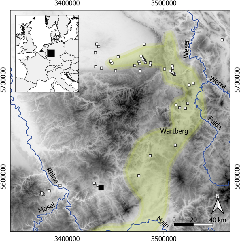
Figure 1 Relief map of central Germany. Locations of Niedertiefenbach (black square) and other gallery graves (white squares) and the main distribution area of Wartberg sites (after Raetzel-Fabian Reference Raetzel-Fabian2000: fig 141). Coordinates: EPSG 31467.
Archaeogenetic analysis of a large proportion of the Niedertiefenbach assemblage, including human remains and dental calculus, is ongoing. So far, genome-wide sequences have been recovered from 42 individuals, which confirm the continuing presence in the late 4th millennium cal BC of relatively isolated groups descended from Mesolithic hunter-gatherers, with significant genetic admixture with the descendants of the first farmers (already established in central-western Germany in the 6th millennium) occurring only in the earlier 4th millennium (Immel et al. accepted). Nevertheless, the region has always been influenced by supra-regional archaeological groups, e.g. Rössen or Michelsberg (Dammers Reference Dammers2003; Jeunesse Reference Jeunesse2010). Around the turn of the 4th millennium, influenced by late Michelsberg, this region became the nucleus of what would later form the Wartberg culture (Raetzel-Fabian Reference Raetzel-Fabian2002a).
Rinne et al. (Reference Rinne, Fuchs, Muhlack, Dörfer, Mehl, Nutsua and Krause-Kyora2016) obtained 15 AMS dates on stratified human bones from Niedertiefenbach, which almost fitted a sequence based on the 10 arbitrary layers and suggested a potentially long chronology for burial activity between ca. 3350 and ca. 2900 cal BC. The authors rejected radiometric dates obtained previously on human bone(s) (layer 5 KN-2771, 4170 ± 60 BP; layer 7 KN-2772, 4140 ± 55 BP; layer 10 KN-2773, 4250 ± 50 BP), which Raetzel-Fabian (Reference Raetzel-Fabian2002b) had used to propose a shorter and later chronology (ca. 2900–2700 cal BC). However, neither of these chronologies is consistent with the 25 new AMS dates reported by Immel et al. (accepted) and 18 additional dates reported here, which place all the burials on the calibration plateau in the late 4th millennium cal BC.
MATERIALS AND METHODS
Skeletal and Morphological Analysis
The original osteological analysis of the approximately 1600 commingled human bones (Czarnetzki Reference Czarnetzki1966) recorded at least 177 individuals, of whom 72 were attributed to age-at-death classes, including 17 sub-adults, 30 younger adults (aged 20–40), 11 mature adults (over 40), and 14 undifferentiated adults (aged 20+). If this sample is representative, the median age-at-death was about 29, and more than half the burial population was aged between 20 and 40. As the new aDNA samples are petrous bones and teeth, often without further individual context, osteological information sometimes remains vague, expressed in large age spans (20–60 years) or tendencies in morphological sex (e.g. female more probable than male). Some bones could not be attributed to specific individuals, but the risk of inadvertently sampling the same individual (e.g. right and left petrous bone) is very low. Where aDNA was well-preserved, this possibility could be completely excluded.
Sample Selection
Given the long burial chronology proposed by Rinne et al. (Reference Rinne, Fuchs, Muhlack, Dörfer, Mehl, Nutsua and Krause-Kyora2016), and considering the circumstances of the excavation, it was planned to directly date every bone or tooth selected for aDNA analysis. The first set of 16 samples (KIA-52267–52282) included a medieval tooth (KIA-52271, 367 ± 25 BP), but the other 15 gave results statistically consistent with a single 14C age, in contrast to the >200 14C year range among results from 15 individuals reported by Rinne et al. (Reference Rinne, Fuchs, Muhlack, Dörfer, Mehl, Nutsua and Krause-Kyora2016). To investigate this perplexing pattern, 5 of the 2016 samples were re-dated in Kiel, and 3 of new samples were replicated in Poznan. Twenty further samples were subsequently chosen for dating, based on aDNA results, of which half were dated in Kiel, and half were dated at the Center for Isotope Research, Groningen University, the Netherlands.
Radiocarbon Analysis
Collagen was extracted following standard acid-alkali-acid protocols, with only slight differences between laboratories. At room temperature, crushed bones were demineralized in HCl, treated with NaOH to dissolve secondary organic compounds, and re-acidified in HCl, before gelatinization overnight in a hot (75–85°C) pH3 solution, and filtration to remove insoluble particles. At Poznan, the filtered collagen was then ultra-filtered, following Brock et al. (Reference Brock, Higham, Ditchfield and Bronk Ramsey2010), to remove low-molecular-weight collagen fragments.
Collagen extracts were freeze-dried and combusted, and the resulting CO2 was reduced to graphite for measurement by accelerator mass spectrometry (AMS). Kiel used a 3 MV HVEE Tandetron AMS, in operation since 1995 and upgraded in 2015. Groningen used a 180 kV IonPlus Micadas AMS system, installed in 2017. At Poznan, samples were dated either on an NEC 1.5 MV Pelletron AMS used since 2001, or a second compact NEC system installed in 2013. All the AMS systems measure 12C, 13C and 14C ion currents from each graphite target simultaneously; the 13C/12C ratio (AMS δ13C) is used to normalize the 14C current for natural and instrumental fractionation, and thus to calculate conventional 14C ages. The reported 14C age errors incorporate uncertainties in measurement, standard normalization, instrumental background, blank correction, and additional uncertainty arising from sample pretreatment, based on long-term experience with laboratory standard and known-age samples of similar materials.
Stable Isotopes
Some of the remaining collagen from each sample was sent for EA-IRMS (elemental analysis-isotope ratio mass spectrometry), to isolab GmbH, Schweitenkirchen, Germany, for measurement of %C, %N, %S, δ13C, δ15N and δ34S (Sieper et al. Reference Sieper, Kupka, Williams, Rossmann, Rummel, Tanz and Schmidt2006). Stable isotope results (δ13C, δ15N and δ34S) are expressed using δ notation (δ = [(Rsample/Rstandard–1)]×1000, and R = 13C/12C, 15N/14N, or 34S/32S) in parts per mille (‰) relative to international standards, Vienna PeeDee Belemnite for δ13C, air N2 for δ15N, and Canyon Diablo Troilite for δ34S. The results (Appendix 1) are averaged measurements of four aliquots of each sample, with standard deviations <0.1 ‰ for δ13C and δ15N, and <0.4 ‰ for δ34S. Final measurement uncertainties are therefore probably better than ± 0.1 ‰ for δ13C and δ15N, and ± 0.2 ‰ for δ34S. One sample, KH150629, did not give enough collagen for EA-IRMS measurement at isolab, but EA-IRMS data (%C, %N, δ13C and δ15N) were obtained during dating at Groningen, with estimated uncertainties of ± 0.1 ‰ for δ13C and ± 0.3 ‰ for δ15N.
PRIOR INFORMATION
Stratigraphy
Although the human remains were excavated in arbitrarily defined layers, numbered 10 to 1 from the earliest to the latest, the depositional sequence was not uninterrupted, as up to three layers of rocks and earth could be distinguished between layers 8 and 4 (Pape Reference Pape2019). These rubble layers separate the inhumations into earlier and later phases. Burials in layer 5 and above clearly belong to the later phase. As detailed stratigraphic subdivision of the earlier burials is difficult to justify from the available documentation, we have treated layers 10 to 6 as one earlier phase. A significant number of human remains, including some dated samples, were not attributed by the excavators to one of the 10 arbitrary layers, and may therefore belong to either the earlier or later phase. Of the bones selected for dating, only KH150618 was from an articulated skeleton (individual 48, layer 4a; Drummer in prep.). Nevertheless, of 1592 bones documented by drawings, 541 were found in articulation. There were at least 47 articulating sets of bones in layers 10 to 6, particularly of lower limb bones. There were also 29 articulations (of e.g. vertebral columns) in layers 5 to 1, suggesting that most bones in these layers were probably from new primary burials. Rinne et al. (Reference Rinne, Fuchs, Muhlack, Dörfer, Mehl, Nutsua and Krause-Kyora2016) suggested that the apparently curated skulls in layer 5a might have been removed from older burials, but these individuals have not been dated.
An important aspect for our model is that the apparent burial sequence constrains the potential dates of death of the individuals concerned, but in most cases the dated sample was a petrous bone, which, due to negligible remodeling after early childhood, effectively dates an event close to the date of birth. If the overall period of burial was relatively brief, therefore, the age-at-death of each individual may be pertinent to whether the calibrated dates are consistent with the burial sequence.
Kinship
In some cases, genetic sequences are sufficiently detailed and similar to demonstrate that the samples analyzed were from related individuals (Immel et al. accepted, Supplementary Figure 5). Here, we focus on the chronological implications. Kinship information (how closely related two individuals were) does not indicate which individual was born first, but it does limit the potential difference between their dates of birth. Various degrees of kinship can be distinguished:
-
First degree kinship (ca. 50% genetic overlap) is shared with a full sibling, child or parent (i.e. individuals with 1st-degree kinship are either born in the same generation, or 1 generation apart);
-
Second degree kinship (ca. 25% genetic overlap) includes a person’s half-siblings, his/her parents’ full siblings, and his/her grandparents or grandchildren (births separated by 0–2 generations);
-
Third degree kinship (ca. 12.5% genetic overlap) includes first cousins, parents’ half-siblings, grandparents’ full siblings, and great-grandparents (births separated by 0–3 generations);
-
Fourth degree kinship (ca. 6.25% genetic overlap) includes relatives separated by 0–4 generations;
-
Fifth degree kinship (ca. 3.13% genetic overlap) includes relatives separated by 0–5 generations.
A human generation is often assumed to be 25 years, but the age difference between parent and child varies widely in ethnographic studies, depending on birth spacing and birth order, as well as the sex of the parent (Fenner Reference Fenner2005). Given that most adults buried at Niedertiefenbach apparently died before the age of 40, we propose that nearly all children were born before their parents reached 30. Fifth-degree kinship would then imply a theoretical maximum separation of 150 years, but this upper limit would only apply to the last-born child in every generation, so it is more realistic to assume that 5th-degree kinship means that two individuals were born less than 120 years apart. The absence of kinship information linking most of the samples analyzed does not mean that these individuals were buried more than 120 years apart, or even that they were contemporaneous but unrelated; variable aDNA preservation may obscures many other kinships.
With archaeogenetic sequences, different algorithms can yield different estimates of the degree of kinship between related individuals (Immel et al. accepted). As kinship only places an upper limit on the differences in date between samples, we have applied the more conservative kinship estimates given by the lcMLkin algorithm (Lipatov et al. Reference Lipatov, Sanjeev, Patro and Veeramah2015), which indicates 5th-degree kinship between pairs of individuals which other algorithms classify as 3rd-degree kin. The chronological model output (see below) would not exclude 3rd-degree kinship in these cases.
RESULTS
14C Ages
All samples dated in Kiel or Groningen gave collagen whose atomic C/N ratio was close to the expected value (3.16–3.32; Szpak Reference Szpak2011), supporting the validity of the 14C, δ13C, and δ15N results (Appendix 1). Samples dated in Poznan were extracted using an ultra-filtration protocol, which may account for the slightly lower collagen yields; %C and %N of the collagen extracts was not reported.
Replication of 8 samples between Kiel and Poznan (Appendix 1) yielded good agreement in 4 cases (differences <1σ), but in 4 cases the differences are unacceptably large (>2σ). The three new Poznan results are consistent with Kiel dates on the same samples, as is one of the 2016 Poznan results. In the four cases of disagreement, the 2016 Poznan results appear to be over-dispersed, perhaps with a bias towards younger ages (Figure 2). A similar range of 14C ages (4300–4500 BP) was reported for the 2016 samples that have not been replicated (Appendix 1). Altogether, 8 of the 15 14C ages reported by Rinne et al. (Reference Rinne, Fuchs, Muhlack, Dörfer, Mehl, Nutsua and Krause-Kyora2016) are below 4420 BP, compared to only 1 of the 43 new results. There is no archaeological explanation for this pattern, and we must assume that all the 2016 results are less reliable than the new dates. We have therefore omitted the 2016 results, except those which are statistically consistent with new results on the same samples. We did not attempt to replicate the radiometric dates rejected by Rinne et al. (Reference Rinne, Fuchs, Muhlack, Dörfer, Mehl, Nutsua and Krause-Kyora2016), which fall even later than the 2016 dates (<4300 BP; see above).
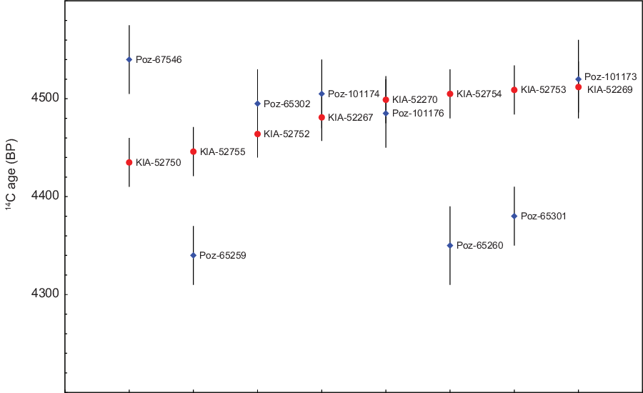
Figure 2 Replication of samples between Kiel and Poznan. For each sample, 14C ages (± 1σ) reported by Kiel (red dot) and Poznan (blue diamond) are shown.
We have not replicated any of the 8 samples dated at Groningen, but the Groningen results are statistically consistent with a single 14C age (T=10.5, T’(5%)=14.1, df=7; [Ward and Wilson Reference Ward and Wilson1978]), and fall within the already narrow range of the 32 results from Kiel. The combined data set (n=40; all Groningen and Kiel results, or weighted mean 14C ages where Poznan and Kiel dates on the same sample are consistent) is inconsistent with a single 14C age, but is still remarkably homogenous (mean 4487 BP, standard deviation 33y; range 4417–4564 BP, interquartile range 4462–4508 BP).
Risk of Dietary Reservoir Effects
Accurate 14C ages from human bones can be misleadingly old, due to consumption of fish and other taxa from aquatic food chains, which are not in full isotopic equilibrium with the atmosphere (“dietary 14C reservoir effects”, or DREs). This phenomenon has been observed at several prehistoric sites in Germany (Fernandes et al. Reference Fernandes, Rinne, Nadeau and Grootes2016), most notably at Ostorf (ca. 3000 cal BC), where human bones have 14C ages 200–800 years greater than those of herbivore tooth pendants from the same burials (e.g. Fernandes et al. Reference Fernandes, Grootes, Nadeau and Nehlich2015).
Although we could only date human remains at Niedertiefenbach, it is inconceivable that the tightly clustered 14C ages could embody such large DREs, as any differences in diet between individuals can realistically only increase the spread of human 14C ages. Smaller DREs (in the order of decades rather than centuries) would be harder to detect, even when comparing human bone and organic grave good 14C ages. Differences in 14C ages less than twice the uncertainty in the difference are statistically insignificant, so the smallest DRE we could measure, if short-lived organic grave goods were available for comparison, is about 60 years. However, the limited range of human 14C ages (about 1.5 times the variation expected if a single bone was dated 40 times, instead of 40 different individuals) restricts the potential variability in DREs. If all 40 individuals were exactly the same date, a scatter of only ± 25 in their DREs would account for the spread of 14C ages; any differences in calendar date between individuals would imply that DREs were even more uniform. The easiest explanation for negligible variation in DREs is that DREs were themselves negligible.
Secondly, aquatic and terrestrial fauna usually have different stable isotope signatures. Variation in human stable isotope values should therefore reflect differential consumption of aquatic and terrestrial species, which must be correlated with differences in DREs. The Niedertiefenbach 14C ages appear to be independent of all three stable isotopes measured, δ13C, δ15N, and δ34S (Figure 3). Although 14C ages are only a crude proxy for DREs, as some of the variation in 14C ages must be due to differences in calendar date, the absence of any visible relationship between 14C ages and stable isotope values is reassuring. Moreover, we do not observe correlations between any of the stable isotopes, which should be correlated if fish had a distinct multi-isotopic signature and fish consumption varied significantly between individuals. Again, the easiest way to minimize differences between individuals in fish consumption is for fish to have been a negligible component of all diets.
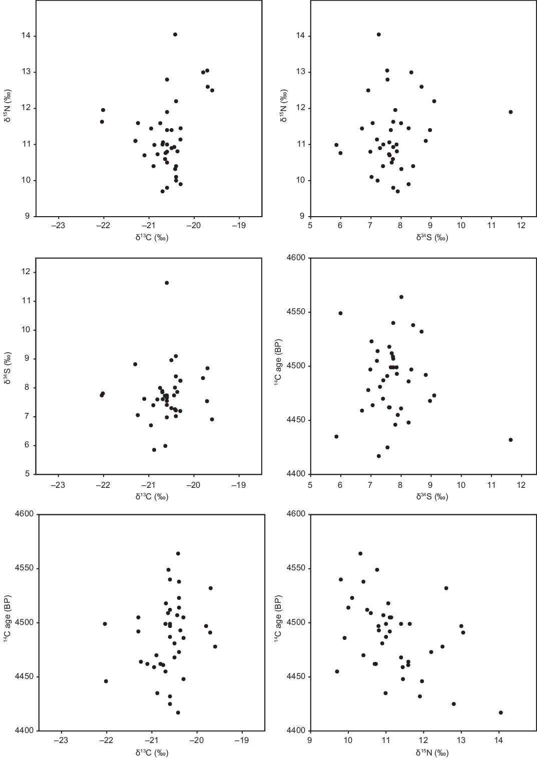
Figure 3 Isotopic results (Appendix 1), showing no apparent correlation between any pair of stable isotopes, or between any stable isotope and 14C age.
Finally, the δ13C and δ15N results are compatible with largely or fully terrestrial diets, based on plants using the C3 photosynthetic pathway (no C4 or CAM plants are known from central Europe at this date). We do not have local isotope reference data from contemporaneous fauna (terrestrial or aquatic), but the human δ13C and δ15N values could be obtained from diets based on the reference terrestrial fauna sampled by Münster et al. (Reference Münster, Knipper, Oelze, Nicklisch, Stecher, Schlenker, Ganslmeier, Fragata, Friederich, Dresely, Hubensack, Brandt, Döhle, Vach, Schwarz, Metzner-Nebelsick, Meller and Alt2018: fig.2) in Sachsen-Anhalt. Some Niedertiefenbach δ15N values are relatively high (> 12 ‰), but in each case the bone sampled was the pars petrosa. Petrous bone isotope values reflect diet in early childhood (Jørkov et al. Reference Jørkov, Heinemeier and Lynnerup2009), and δ15N variation among petrous bone samples in this assemblage probably reflects differences in weaning age (see e.g. Münster et al. Reference Münster, Knipper, Oelze, Nicklisch, Stecher, Schlenker, Ganslmeier, Fragata, Friederich, Dresely, Hubensack, Brandt, Döhle, Vach, Schwarz, Metzner-Nebelsick, Meller and Alt2018: fig.5). Because petrous bone collagen forms rapidly, some isotopic variation between samples may also reflect short-term environmental changes (due to weather, grazing locations, farming practices etc.). Isotope values from adult skull fragments (n=8), which reflect average diets throughout adulthood, appear to represent similar, terrestrial-based diets (mean ± s.d. δ13C –20.9 ± 0.5 ‰, δ15N 11.2 ± 0.4 ‰), and given the range of 14C ages from skull samples (4435–4512 BP), it is unlikely that the petrous bone 14C ages (4417–4564 BP) are affected by significant DREs.
Sulfur Stable Isotopes
All 39 samples for which we have δ34S data met the acceptance criteria for mammal collagen recommended by Nehlich and Richards (Reference Nehlich and Richards2009) (%S 0.15–0.35%; atomic C/S 300–900; atomic N/S 100–300), so we are confident that the δ34S results are valid. Given the lack of evidence of DREs, the best explanation for δ34S differences is mobility (Nehlich et al. Reference Nehlich, Oelze, Jay, Conrad, Stäuble, Teegen and Richards2014; Nehlich Reference Nehlich2015). Again, the 8 skull samples gave similar results (mean ± s.d. 7.2 ± 0.6‰), which presumably represents a local average. Nehlich (Reference Nehlich2015: fig.7) shows similar δ34S values in archaeological bone collagen from sites across inland Germany, including Hesse. The one real outlier (KH150637, δ34S 11.6 ‰) is from the petrous bone of an older man, who may have lived elsewhere in childhood. Nehlich (Reference Nehlich2015: fig.7) shows higher δ34S values (> 10‰) to the north of Niedertiefenbach, so this interpretation is feasible. Mobility in other directions would be difficult to detect or exclude, as the sulfur isoscape appears to have been more uniform.
Chronological Modeling
Individually, the calibrated 14C ages date all 40 burials to the calibration plateau spanning the last third of the 4th millennium cal BC (Bronk Ramsey Reference Bronk Ramsey2009; Reimer et al. Reference Reimer, Bard, Bayliss, Beck, Blackwell, Bronk Ramsey, Buck, Cheng, Edwards, Friedrich, Grootes, Guilderson, Haflidason, Hajdas, Hatte, Heaton, Hoffmann, Hogg, Hughen, Kaiser, Kromer, Manning, Niu, Reimer, Richards, Scott, Southon, Staff, Turney and van der Plicht2013). If we use OxCal’s kernel-density estimation model to summarize the dates (Bronk Ramsey Reference Bronk Ramsey2017), or apply a simple bounded-phase Bayesian chronological model (assuming these dates represent a uniform, continuous phase of burial activity), potential dates after ca. 3100 cal BC are excluded (Figures 4 and 5), but the modeled date of each individual still spans >ca. 200 years, and the estimated duration of burial activity is imprecise (Figure 6). Incorporation of the more detailed prior information (above) provides a much more precise date for each individual (Figure 7), with a correspondingly better estimate of the duration of burial (Figure 8). The exact code in OxCal v.4’s Chronological Query Language (Bronk Ramsey Reference Bronk Ramsey2009) for all models is provided in Supplementary Information.
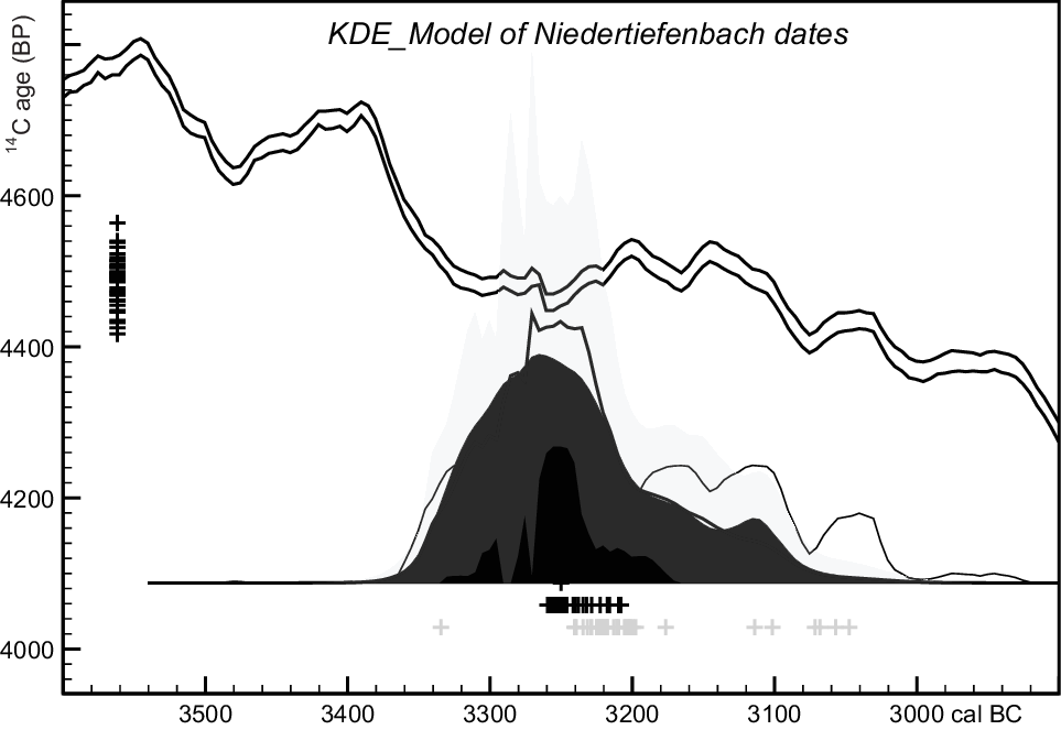
Figure 4 Kernel-density estimate summarizing the dates of 40 individuals, using the OxCal function KDE_Model with default parameter values (Bronk Ramsey Reference Bronk Ramsey2017). Black crosses show (left) median uncalibrated 14C ages and (below) median modeled calibrated dates (which span 3340–3090 cal BC at 95% probability in nearly all cases). Gray crosses represent median calibrated dates before KDE modeling. The relevant section of the IntCal13 calibration curve (Reimer et al. Reference Reimer, Bard, Bayliss, Beck, Blackwell, Bronk Ramsey, Buck, Cheng, Edwards, Friedrich, Grootes, Guilderson, Haflidason, Hajdas, Hatte, Heaton, Hoffmann, Hogg, Hughen, Kaiser, Kromer, Manning, Niu, Reimer, Richards, Scott, Southon, Staff, Turney and van der Plicht2013) is shown for reference.

Figure 5 Simple bounded-phase model of the dates of 40 individuals, obtained using the Boundary and Phase functions in OxCal v.4.3 (Bronk Ramsey Reference Bronk Ramsey2009). For each sample, the probability density function of the simple calibrated date is shown in outline, while the model’s posterior density estimate of the sample date is shown in black. The distributions start boundary and end boundary are calculated by the model, which, due to the multimodal calibrated dates, is unable to resolve whether burial activity ended ca. 3200 cal BC or after 3100 cal BC. Nevertheless, the dates are compatible with the model structure (Amodel=75.1).
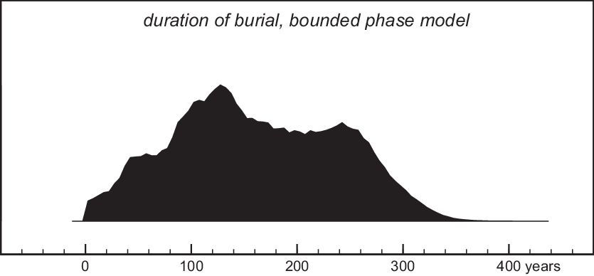
Figure 6 Estimated duration of burial activity, bounded-phase model (Figure 5).
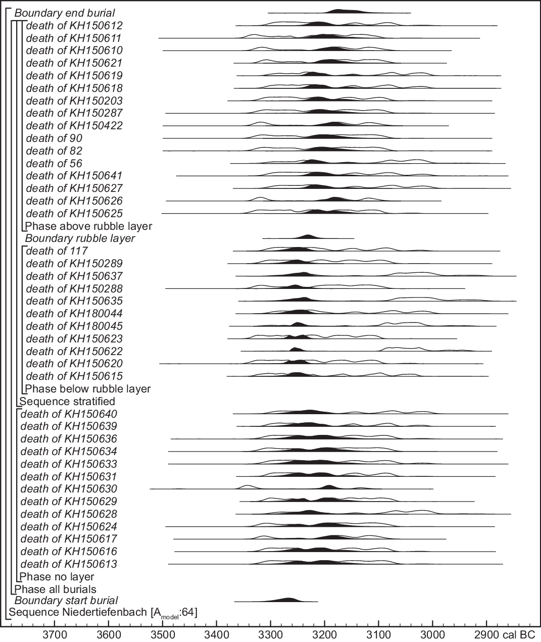
Figure 7 Preferred chronological model. The format is the same as that of Figure 3, but burials in layers 10 to 6 are required to predate the rubble layer and burials from layers 5 to 1. Small offsets are applied to the calibrated dates to account for age-at-death and collagen-turnover time, and the birth dates of related individuals are constrained by potential generational differences permitted by their degree of kinship. Full details are given in Supplementary Information.
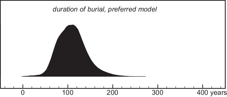
Figure 8 Estimated duration of burial activity in preferred model (Figure 7).
In order to use both the kinship information (which constrains the potential difference in dates of birth between related individuals) and stratigraphic relationships (which reflect relative dates of death), the Figure 7 model has to account for the lifespans of dated individuals. Most dated samples were petrous bones, whose collagen content should correspond to the first 5 years of life (at most), whereas collagen in the cranium is slowly and continuously remodeled throughout life (Calcagnile et al. Reference Calcagnile, Quarta, Cattaneo and D’Elia2013). As most individuals appear to have died at 20–40 years of age, the model assumes that the date of death was 25 ± 7 years after the date of a petrous bone sample, and 15 ± 7 years after the date of a cranium sample (unless we have more specific age-at-death information). The model assumes that individuals from layers 10 to 6 (below the rubble layer) died and were buried before those in stratigraphically later layers 5 to 1.
Kinship information concerns 14 dated samples (Appendix 1, Figure 9). Kinship relationships do not indicate birth sequence and stratigraphy does not determine which individual was born first (the grandparent of a child buried in layer 10 could have been buried above the rubble layer). Kinship only provides an upper limit to the possible difference in date of birth. Our model uses OxCal’s Span function to restrict differences in date between petrous bone samples from related individuals, whose dates are cross-referenced with their dates of death in the stratigraphic sequence. Third-degree kinship is assigned a Span of <80 years, 4th-degree <100 years, and 5th-degree <120 years. Three infants with 1st-degree kinship, KH150620, KH150622 and KH150623, must have been full siblings, so we limited their difference in date to <15 years.
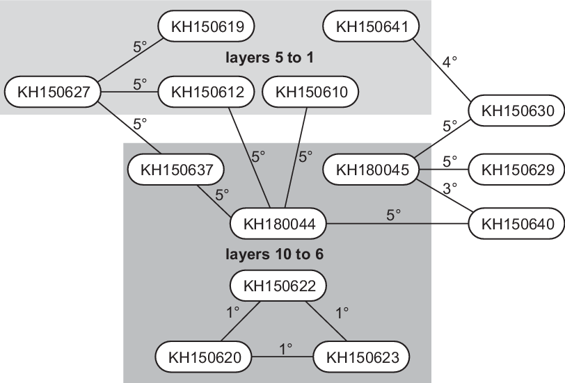
Figure 9 Kinship degrees between dated samples (redrawn from Immel et al. [accepted] Supplementary Figure 5). Samples KH150629, KH150630 and KH150640 were not assigned to an excavation layer.
The model (Figure 7) has good overall agreement (Amodel=64, >60), without omitting or down-weighting any sample. One result (KIA-53048, 4417 ± 19) is a poor fit for its position in the model (A=15.7), but two graphites made from separate combustions of the same collagen extract gave almost identical measurements (4412 ± 24, 4424 ± 28), so this result (their weighted mean) is not a measurement outlier. This sample (KH150622) is from the sister of two other individuals from layer 10 (see above), so it cannot be intrusive from a later phase of burial activity, after 3100 cal BC, as simple calibration might suggest. Omitting it raises the overall index of agreement but has a negligible effect on the resulting chronology.
Unlike the simple bounded-phase model (Figure 5), our preferred model (Figure 7) gives unimodal estimates of the dates of the start and end of burial activity (and therefore of its duration), as well as of the date of the rubble layer between layers 6 and 5. Burials predating this layer took place in the mid-33rd century cal BC. The rubble was deposited in the later 33rd century and burials overlying the rubble layer continued until the early-mid 32nd century. Thus, burial activity probably lasted 3–6 generations (70–140 years, >68% probability; Figure 8). Individuals who cannot be attributed to an excavation layer are in most cases only datable to the overall period of burial, but in a few cases, the combination of kinship and the wiggles of the calibration curve lead to much more precise dates.
Sensitivity Analyses
Reproducibility is rarely discussed in publications of Bayesian chronological models. In order to validate the preferred model output, we tested its robustness and its dependence on various components of the model following three approaches: using the same prior information as in the preferred model, but varying the likelihoods (the calibrated dates included in the model); using the same likelihoods as in the preferred model, but omitting some of the prior information; and using the full prior information on simulated 14C data sets corresponding to different calendar date ranges. Full details are given in Supplementary Information.
Varying the Likelihoods
The preferred model includes the 2016 Poznan results (Rinne et al. Reference Rinne, Fuchs, Muhlack, Dörfer, Mehl, Nutsua and Krause-Kyora2016) only if they have been successfully replicated. Including the 2016 results from samples which have not been replicated would double the estimated duration of burial activity, but one result (Poz-65258, 4305 ± 35 BP) would still fit the model so poorly (A=3%) that it would normally be excluded; the model would then give a bimodal estimate for the end date, and therefore for the duration of burial activity. As the longer chronology (>200 years of burial activity) depends on the inclusion of unreplicated 2016 results, and only 1 of the 5 2016 results from replicated samples was consistent with a second date on that sample, the shorter chronology given by the preferred model is clearly more credible.
The risk of DREs at Niedertiefenbach appears to be minimal (see above), but the calibration plateau means that minor 14C offsets could significantly affect calibrated dates. To gauge the potential impact of undetected DREs on our chronology, we generated a randomized DRE correction for each 14C date in the preferred model, within a prescribed range (see Supplementary Material). Small randomized DRE corrections (below ca. 30 14C years) are compatible with the preferred model structure and do not significantly alter the resulting chronology. Larger randomized DRE corrections (which can produce longer and/or later chronologies) are inevitably incompatible with the prior information incorporated in the model (i.e. produce an overall index of agreement well below the normal threshold value of 60). More uniform DRE corrections, however unrealistic (e.g. a single Delta_R applied to all the 14C ages), are also incompatible with the model. Whilst these tests do not entirely exclude the risk of minor DREs, with limited variation between individual DREs, our assumption that DREs were negligible is much easier to believe.
The preferred model tries to incorporate differences between samples in collagen-turnover time, which depend on which element was sampled and the individual’s estimated age-at-death. These differences are expressed as calendar-year offsets with normal distributions and 1-sigma uncertainties of ± 7 for most adult burials (i.e. 95% confidence intervals of 28 years). Increasing these uncertainties can lead to extreme model averaging, whereby all samples converge on the same date, producing an estimated overall burial timespan of less than 20 years. This would imply that individuals buried below the rubble layer lived longer than those buried afterwards, which is not supported by the skeletal evidence.
Varying the Prior Information
With no informative priors, we are unable to date the burials more precisely than ca. 3340–3090 cal BC (see above; Figures 4 and 5). The preferred model incorporates two types of informative prior information, the maximum differences in date of birth for related individuals (kinship constraints), and the stratigraphic sequence of burials earlier and later than the rubble layer.
Kinship should have limited impact, if the overall burial sequence spanned only 3–6 generations, as any two individuals selected at random would probably not have been separated by more than 3 generations anyway; the uniform deposition assumption incorporated in the use of phase boundaries would thus in practice predict similar age differences to the kinship constraints. Nevertheless, a model which incorporates the stratigraphic sequence and age-at-death offsets, but not kinship constraints, yields bimodal estimates for the end of burial activity (peaks ca. 3160 and 3060 cal BC), and is therefore compatible with both shorter (<100y) and longer (>200y) chronologies.
On the other hand, a model incorporating kinship information, but not the stratigraphic sequence, favours a short chronology in the early 33rd century, in contrast to any model incorporating the stratigraphic sequence. Thus the validity of the stratigraphic sequence is crucially important, but a model which requires burials above the rubble layer to predate those below it is almost compatible with the calibrated dates (Amodel=53.8), and is almost as good a fit as the model with no stratigraphic sequence (Amodel=56.5). Therefore, the 14C results do not validate the assumed stratigraphic sequence, because they do not force us to reject demonstrably wrong sequences. The assumption that dated samples from layers 5 to 1 are not redeposited from layers 10 to 6, which is based on the frequency of articulations in the upper layers, remains critical to the model output.
Simulating Different Calendar Date Ranges
Synthetic 14C ages were generated using OxCal’s R_Simulate function, which requires each sample’s calendar date and 14C-age measurement uncertainty to be specified in the model code (Supplementary Information) and yields a different 14C age every time the model runs. If enough samples have been dated, however, overall model output will be reproduced consistently. By varying the calendar ages of simulated 14C samples, we also investigated the influence of the calibration curve or the duration of a sequence on model output (i.e. on whether modeled dates were accurate, precise, reproducible and consistently unimodal).
The first simulated data set aimed to check the reproducibility of the preferred model output. Calendar dates for all 40 individual deaths were generated by randomly sampling a range (mean ± 1σ) derived from the preferred model’s posterior density estimate of the date of that burial. The same prior information was applied as in the preferred model. Repeated runs of this simulation model consistently dated the burials to a ca. 100-year range centered on the later 33rd century cal BC, in agreement with the randomized dates used and with the preferred model output. Thus, the preferred model output appears to be reproducible.
The second and third data sets were created by moving the calendar dates of samples in the first data set 50 years earlier and later respectively, to check whether the preferred model output was an artefact of the shape of the late 4th millennium calibration plateau. No model run using either the earlier or later data produced output comparable to that of the preferred model, however. The earlier data set strongly favored solutions in the late 3300s and early 3200s cal BC, while the later data set gave answers centered on the 3100s, in agreement with the “known” calendar dates of burials in these data sets. Therefore, it is not plausible that the preferred model chronology would be centered on the late 3200s if the true dates of the Niedertiefenbach burials were more than a few decades earlier or later.
To visualize the impact of the calibration plateau on model output, we ran the preferred model simulation with the dates shifted 500 years and 2000 years later. With the model centered on the mid-2700s cal BC, it was difficult to exclude dates around 2900, leading to bimodal estimates; in terms of providing consistently accurate, precise and unimodal estimates of the dates of key events, it did not perform any better than the simulation model of the real chronology, centered on the later 3200s. In the late 2nd millennium, where the calibration curve is relatively monotonic, model output was sometimes more precise than that of the Niedertiefenbach preferred model, but often the model converged on a single date. Thus, the calibration plateau in the late 4th millennium appears almost irrelevant to the accuracy, precision and reproducibility of model output.
The last simulated data set aimed to test whether the duration of burial activity was estimated accurately by the preferred model. The first simulated data set showed that the duration estimated by the preferred model was reproducible, but to check its accuracy we stretched the first simulated data set by doubling the gap between the median calendar date of all samples and the date of each sample, giving a data set spanning >150 years. Maximum date differences permitted by kinship were also doubled, to reflect the fact that stretching the data set should have doubled the gaps between dates of individual samples. The stretched model estimates were less precise, but all model runs gave much longer estimates of duration than the preferred model.
Archaeogenetic kinship information is restricted to 5th degree or closer relationships, so in a genuine case-study, the only kinship constraints available would limit date differences between related individuals to 5 generations. If kinship constraints in the stretched model were limited to 5 generations, most runs yielded much shorter and less accurate chronologies (often <50 years duration). As most of the Niedertiefenbach individuals are not (demonstrably) linked by kinship, there is arguably a risk that the burial chronology was longer than indicated by the preferred model, in which demonstrated kinship between a small number of individuals might have been overly influential. However, we note that the unimodal peak in the preferred model estimate of the duration of burials corresponds to one peak in the bimodal duration estimated when all kinship constraints are removed, whereas the spuriously short durations obtained when the stretched model kinship constraints are limited to 5 generations are entirely inconsistent with the longer and more realistic durations estimated when no kinship constraints are applied. Therefore, the preferred model duration is probably realistic. We did not test longer chronologies centered on earlier or later dates, as the Niedertiefenbach burial sequence cannot have started much earlier than 3300 cal BC, or have finished after 3100, because if it did there would inevitably be many 14C ages outside the range of those included in the preferred model.
DISCUSSION
The Chronology of Burial at Niedertiefenbach
The preferred chronological model (Figure 7) uses all available information and provides unimodal and relatively precise estimates for the dates of interest, spanning ca. 3–6 generations (70–140 years, 68% probability) between the early-mid 3200s and early 3100s cal BC.
A critical assumption, which cannot be tested by the results, is that 10 of the dated burials pre-date the rubble layer, and 16 postdate it. Without this stratigraphic sequence, all the burials might date to under a century in the late 3300s and/or early 3200s. Articulating groups of bones account for 34% of the assemblage, so we believe that few, if any, of the dated bones found in layers 5 to 1 are derived from individuals originally buried beneath the rubble separating layers 6 and 5. Even with the stratigraphic sequence, kinship is useful in constraining the end of burial activity, and thus the duration of burial; without kinship we would be unable to choose between a 70–140 year span and a long chronology lasting 200–250 years.
Another important assumption is that dietary reservoir effects were negligible. DREs below ca. 40 14C years would not be detectable and would barely affect the model output. Much higher or more variable DREs seem unlikely, given the narrow range of 14C ages and the stable isotope results.
The preferred model provides relatively precise dates for each sample. In looking for temporal patterns within the assemblage, we cannot observe trends in aspects such as pathologies, which are not recorded for most of the dated individuals, but several attributes can be analyzed. There are approximately twice as many males as females among the 77 cases where the sex was determined by aDNA (Immel et al. accepted), and a similar sex ratio prevails among the dated samples (Appendix 1). However, the female burial dates appear to be evenly distributed within the overall period of burial (Figure 10), and do not suggest that female burials took place over a shorter period than male burials.

Figure 10 Posterior density estimates of the dates of death of females, and overall start and end of burial activity, extracted from the preferred model (Figure 7).
Stable isotope data are available for all dated individuals. δ13C and δ15N values show no obvious trends, presumably because δ15N variation is related mainly to weaning age, and δ13C values are too tightly clustered (half fall between –20.7 and –20.4‰). Although several individuals gave relatively high δ34S values (>8.4 ‰, i.e. >2σ above the average for skull bone samples), only KH150637 (which is the clearest isotopic outlier) is likely to predate the gallery grave (Figure 11). In this case, KH150637 might be regarded as a founder of the Niedertiefenbach community. KH150610, KH150618 and KH150641 all appear to have been born after the start of burial at Niedertiefenbach and might indicate ongoing contact with the home region of KH150637.
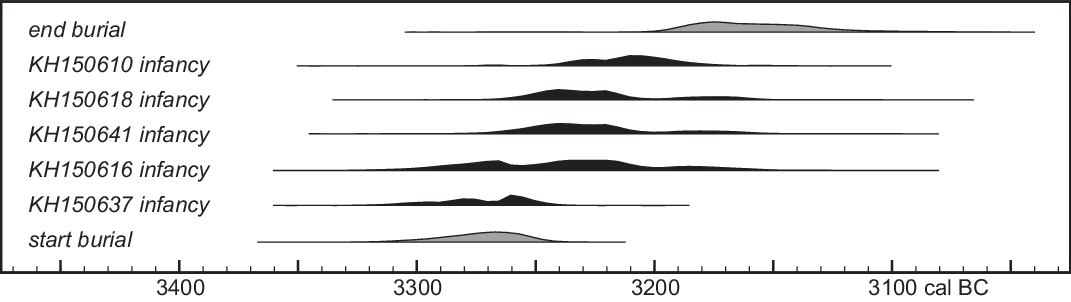
Figure 11 Posterior density estimates of the dates of individuals with non-local (>8.4 ‰) δ34S values, compared to overall burial chronology. These distributions, extracted from the model shown in Figure 7, are for the date of collagen formation in the petrous bone (i.e. when the non-local δ34S signal was acquired) rather than the burial date of the individual concerned.
Archaeogenetic analyses (Immel et al. accepted) reveal additional attributes that might be chronologically sensitive, such as the incidence of mitochondrial or Y-chromosome haplogroups, or of alleles associated with skin, hair or eye color, or lactose and starch tolerance. The haplogroups are so diverse that the number of dated individuals in each haplogroup is too small to show clear temporal patterns. The most common, Y-chromosome haplogroup I2c1a1, is represented by 9 individuals (including the non-local “founder” KH150637), whose birth dates appear to have spanned the entire range of birth dates of the Niedertiefenbach burials (Figure 12; such patterns might imply that patrilocal residence was the norm in Wartberg society). Conversely, the population is relatively uniform in terms of alleles associated with particular phenotypes; only lactose-intolerant individuals are known, for example, and nearly all cases the same allele for darker skin/hair color was identified. Most individuals appear to have had brown eyes; the three cases of blue eyes appear to date to the middle of the date range for brown-eyed individuals. Thus, we have not detected any genetic shifts over the relatively short period covered by the burials.
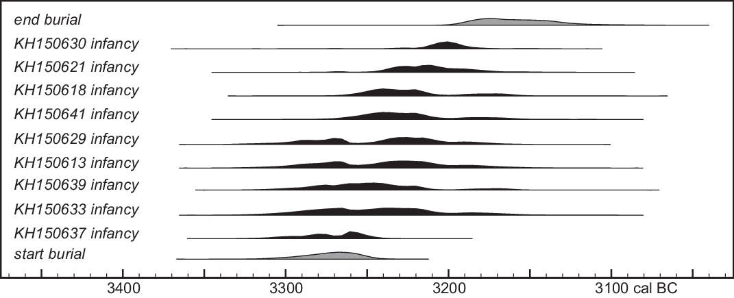
Figure 12 Posterior density estimates of the dates of of individuals with Y-chromosome haplotype I2c1a1 (Immel et al. accepted), compared to overall burial chronology. These distributions, extracted from the model shown in Figure 7, are for the date of collagen formation in petrous bone, rather than the burial date of the individual concerned. Within estimate uncertainty, no other dated individual appears to predate KH150637 or postdate KH150630.
The burial population is unknown, due to the destruction of most of the gallery grave in the 19th century, but extrapolating from the excavated area, it is possible that 400 or more individuals were buried at Niedertiefenbach (Rinne et al. Reference Rinne, Fuchs, Muhlack, Dörfer, Mehl, Nutsua and Krause-Kyora2016: 295). The timespan covered by the dated burials almost certainly underestimates the overall period of activity, however, as all the dated samples were from one end of the grave, opposite the entrance. Accurate estimation of the size of Niedertiefenbach community is therefore challenging. Nevertheless, the average live population could easily have been ca. 100, or more if other burial practices occurred simultaneously.
Implications for Chronological Modeling on Calibration Plateaus
Bayesian chronological modeling aims to provide date estimates which include the true date of an event, are more precise than simple calibrated dates, and which are reproducible. Otherwise, chronological models can do more harm than good. Ideally, model output would also be unambiguous, but we cannot remove the wiggles in the calibration curve, which often lead to multimodal solutions. The same prior information and data quantity and quality can thus provide more or less useful chronologies at different absolute dates, due to the calibration curve itself.
However, the Niedertiefenbach case shows that a calibration plateau is not necessarily a barrier to accurate, precise and reproducible chronologies. The start and end boundaries in our preferred model are dated to within 70–80 years at 90–95% probability, some individuals are dated to within 60 years at >90% probability, and the rubble layer is dated to within 30 years at >80% probability, which is a precision comparable to that achievable by Bayesian models on steeper sections of the calibration curve (e.g. Bayliss et al. Reference Bayliss, Bronk Ramsey, van der Plicht and Whittle2007: fig.11; Czerniak et al. Reference Czerniak, Marciniak, Bronk Ramsey, Dunbar, Goslar, Barclay, Bayliss and Whittle2016: fig.5). These estimates appear to be robust.
Paradoxically, given traditional misgivings about 14C dating on calibration plateaus, accuracy may be more challenging than precision. The validity of prior information is always critical, but on calibration plateaus, calibrated dates usually cannot contradict false priors. Sensitivity testing of model output against permutations of the prior information is therefore even more important. The accuracy of 14C ages, and of their reported uncertainties, is also critical when working with calibration plateau chronologies, as small 14C age offsets can lead to large shifts in calibrated date. Bayesian models on calibration plateaus are particularly sensitive to minor reservoir effects or low levels of sample contamination.
Our model is not tightly constrained by prior information (only 26 of the 40 samples are attributed to either an earlier or later phase, based on stratigraphy, and only 14 of the 40 dated individuals are related, mainly by 3rd–5th degree kinship), but it combines a sequence of two phases with constraints on potential differences in date between some samples. This combination of ordered events with limited date differences is also essential to wiggle-matching and deposition models, and it appears to be more useful in the Niedertiefenbach case than either a more detailed sequence (e.g. a 10-layer sequence without kinship gives much lower precision than the preferred model) or a more constrained duration (without the sequence, the model gives multimodal start and end dates even if the overall duration is set to 100 ± 15 years).
CONCLUSION
As 14C measurement precision has improved, the term calibration plateau no longer means an interval of several centuries which cannot be further subdivided; rather it is an interval in which a calibrated 14C date typically has a multimodal distribution, which offers several multi-decadal solutions spanning several centuries, but also effectively rules out many potential dates within this range. If we can use a Bayesian modeling approach to exclude some solutions, it is possible to date events on a plateau as precisely as in periods where the calibration curve is monotonic and/or steep. The challenge is to avoid excluding the true dates of samples. Accurate 14C ages are one prerequisite; another is that prior information is not just valid but is pertinent to both the order and the duration of events.
At Niedertiefenbach, we have shown that a genetically diverse community continued to use the same gallery grave for several generations in the 3200s and early 3100s cal BC. We have not detected any shift in the human gene pool, diet or burial practice within this period, but we have demonstrated that such transformations, if they had taken place, could be recognized and dated at multi-decadal but sub-centennial resolution.
ACKNOWLEDGMENTS
This paper is the result of collaboration between members of CRC1266 Scales of Transformation – Human-Environmental Interaction in Prehistoric and Archaic Societies, Christian-Albrechts University, Kiel, Germany. CRC1266 is funded by the German Research Council (DFG project 2901391021). New radiocarbon and stable isotope analyses were jointly funded by CRC1266 subprojects D2 (Third millennium transformations of social and economic practices in the German Lower Mountain Range; PI C Rinne), F4 (Tracing infectious diseases in prehistoric populations; PIs A Nebel, B Krause-Kyora) and G1 (Timescales of change – chronology of cultural and environmental transformations; PIs J Meadows, T Meier). We thank the staff of all laboratories for their cooperative and professional work, and for fruitful discussions of the results.
SUPPLEMENTARY MATERIAL
To view supplementary material for this article, please visit https://doi.org/10.1017/RDC.2020.76
Appendix 1. AMS and EA-IRMS results
References: 1: (Rinne et al. Reference Rinne, Fuchs, Muhlack, Dörfer, Mehl, Nutsua and Krause-Kyora2016); 2: (Immel et al. accepted); 3: previously unpublished
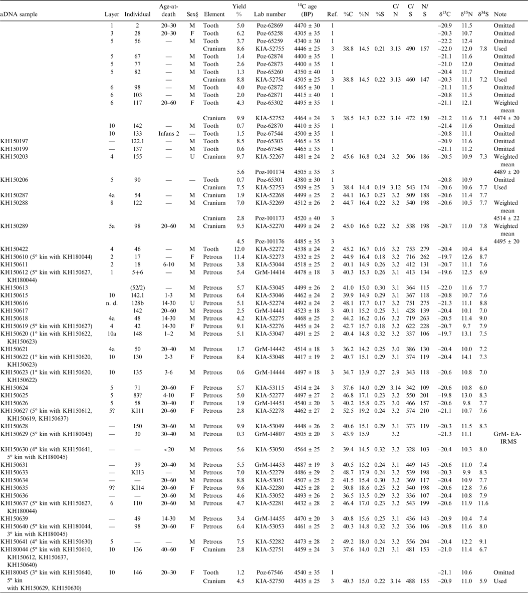
KH150614 and KH150632 (submitted to Groningen) failed to date


 Open access