


Introduction
Radiocarbon dating and its calibration into calendar years is a powerful tool in archaeology and earth sciences, but its precision can be difficult to understand. For example, in dendrochronology, single-year accuracy is achievable and commonly expected. In contrast, understanding the relationship between the raw radiocarbon measurement (with its associated uncertainty) and the calibrated date (with its uncertainty) in radiocarbon dating is more complex.
The first step in establishing a dating strategy is to choose the right sample(s) to characterize an event. This involves taking a holistic view of the scientific question, the nature of the sample (physiology, sedimentary context, etc.) and preservation conditions. They have been extensively investigated in other studies: the recording of several years in bone because of the rate of bone cell turnover (Johnstone-Belford et al. Reference Johnstone-Belford, Fallon, Dipnall and Blau2022), the age span incorporated by an heterogenous sample whose constituent materials are of different origins (Balesdent et al. Reference Balesdent, Basile-Doelsch, Chadoeuf, Cornu, Derrien, Fekiacova and Hatté2018; Calandra et al. Reference Calandra, Cantisani, Conti, Salvadori, Barone, Liccioli, Fedi, Salvatici, Arrighetti, Fratini and Garzonio2024; Dolman et al. Reference Dolman, Groeneveld, Mollenhauer, Ho and Laepple2021), the outgassing of old or even 14C-free CO2 in the vicinity of wetlands and volcanoes and associated to the canopy effect in dense woodlands (e.g. Fontugne et al. Reference Fontugne, Hatté, Tisnérat-Laborde, Ollivier and Kuzucuoğlu2024; Hatté and Jull Reference Hatté and Jull2025; Olsson and Kaup Reference Olsson and Kaup2001; Pasquier-Cardin et al. Reference Pasquier-Cardin, Allard, Ferreira, Hatte, Coutinho, Fontugne and Jaudon1999; Svarva et al. subm.), impact of marine reservoir age directly or through diet (e.g. Olsen et al. Reference Olsen, Heinemeier, Lübke, Lüth and Terberger2010), etc. Of course, all the uncertainties resulting from these factors must be taken into account in the final result. It, however, is not the aim of this article to consider all these elements.
In a similar study focused on the precision of the radiocarbon method, the steep sections of the calibration curve were shown to yield narrow calibrated ranges for individual samples (Svetlik et al. Reference Svetlik, Jull, Molnár, Povinec, Kolář, Demján, Pachnerova Brabcova, Brychova, Dreslerová, Rybníček and Simek2019). In the present work, we aim to explore the calibration potential even further and assess the benefits of high precision for a single radiocarbon measurement. With the benefit of time, we use the newer IntCal20 curve, which, according to its authors, is better defined (Reimer et al. Reference Reimer, Austin, Bard, Bayliss, Blackwell, Bronk Ramsey, Butzin, Cheng, Edwards, Friedrich, Grootes, Guilderson, Hajdas, Heaton, Hogg, Hughen, Kromer, Manning, Muscheler, Palmer, Pearson, van der Plicht, Reimer, Richards, Scott, Southon, Turney, Wacker, Adolphi, Büntgen, Capano, Fahrni, Fogtmann-Schulz, Friedrich, Köhler, Kudsk, Miyake, Olsen, Reinig, Sakamoto, Sookdeo and Talamo2020, their Figure 4).
The aim of this study is to provide a framework where it is easy for a user not versed in the intricacies of radiocarbon calibration to decide if a radiocarbon measurement with a required precision will deliver the needed calibrated range, given the context and the research questions at hand. To do so, we’ll explore the challenges involved in calibrating a single radiocarbon date to the Holocene and to study how the precision of radiocarbon measurements together with the age of the sample (positioning on the calibration curve) influence the final calibrated age range.
Methods
The Holocene epoch was selected because the calibration curve for this period is derived from dendrochronologically dated tree rings, as the IntCal20 calibration curve is fully atmospheric up to approximately 13,910 cal BP (Reimer et al. Reference Reimer, Austin, Bard, Bayliss, Blackwell, Bronk Ramsey, Butzin, Cheng, Edwards, Friedrich, Grootes, Guilderson, Hajdas, Heaton, Hogg, Hughen, Kromer, Manning, Muscheler, Palmer, Pearson, van der Plicht, Reimer, Richards, Scott, Southon, Turney, Wacker, Adolphi, Büntgen, Capano, Fahrni, Fogtmann-Schulz, Friedrich, Köhler, Kudsk, Miyake, Olsen, Reinig, Sakamoto, Sookdeo and Talamo2020). The radiocarbon concentrations are presented in F14C, as defined by Stuiver and Polach Reference Stuiver and Polach1977. Following the radiocarbon convention, in this article, BP means “conventional radiocarbon years before AD 1950,” using the radiocarbon half-life estimated by Libby (Stuiver and Polach Reference Stuiver and Polach1977). To express calibrated radiocarbon ages, the cal BP abbreviation is used.
To analyze the Holocene epoch, radiocarbon dates ranging from 90 to 10,200 BP were converted to F14C and calibrated using the IntCal20 dataset (Reimer et al. Reference Reimer, Austin, Bard, Bayliss, Blackwell, Bronk Ramsey, Butzin, Cheng, Edwards, Friedrich, Grootes, Guilderson, Hajdas, Heaton, Hogg, Hughen, Kromer, Manning, Muscheler, Palmer, Pearson, van der Plicht, Reimer, Richards, Scott, Southon, Turney, Wacker, Adolphi, Büntgen, Capano, Fahrni, Fogtmann-Schulz, Friedrich, Köhler, Kudsk, Miyake, Olsen, Reinig, Sakamoto, Sookdeo and Talamo2020), processed with OxCal (Bronk Ramsey Reference Bronk Ramsey2009) version 4.4 with a resolution of one year using the R_F14C function. Then various levels of precision were allocated, from 0.01% to 0.5%, with a step of 0.005%, resulting in the computation of over 1,000,000 calibrated F14C. The calibrated age ranges considered are at the 95.4% probability level. The data was then analyzed in custom written scripts in Matlab, version R2022b, with the modified Violin Plots package (Hoffmann Reference Hoffmann2024).
The conversion from 14C ages or F14Cs to cal BP may result in multiple possible cal BP ranges due to the non-linear nature of the calibration curve. To determine the full width of the cal BP ranges, we summed the intervals of possible calendar years, which represent 95.4% probability of finding the true date in that range(s). For example, for a radiocarbon date of 1000 ± 30 BP, that is F14C = 0.8830 ± 0.0033 the calibrated range includes two sub-ranges of 58 and 74 years, resulting in a full range of 132 years, as shown on Figure 1. The full range will be referred to as cal BP range through the article.
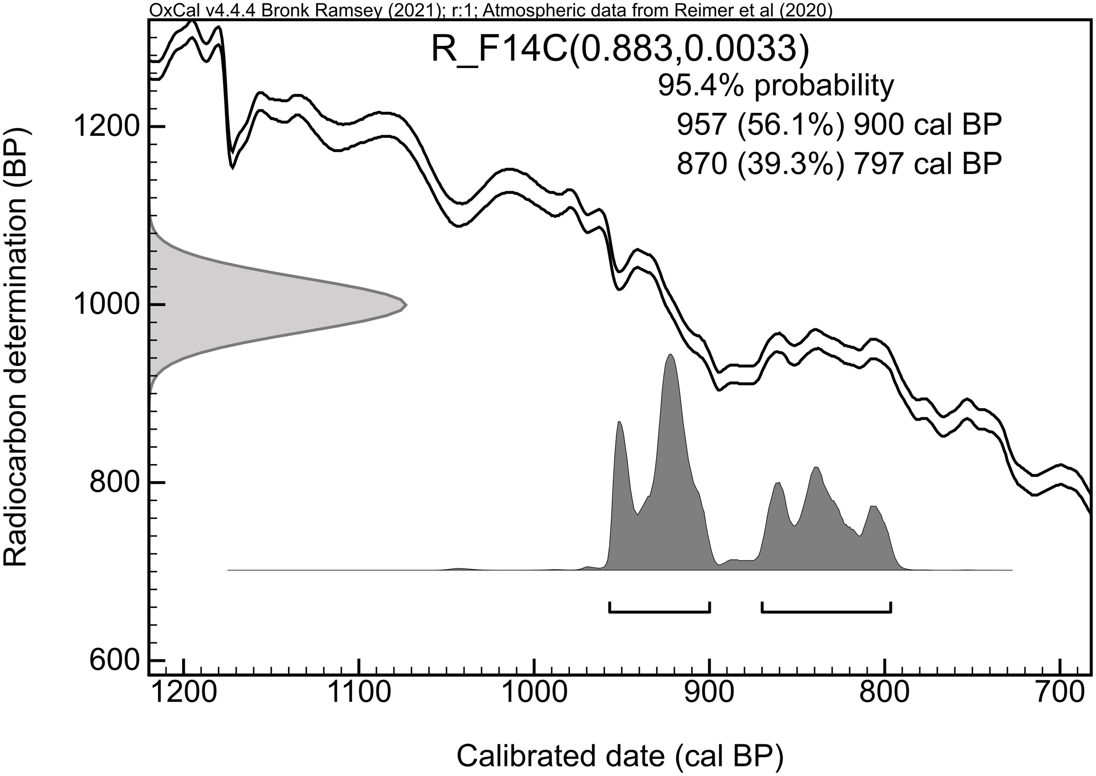
Figure 1. Example of the calibration of the radiocarbon date 1000 ± 30 BP (F14C = 0.8830 ± 0.0033) processed in the OxCal program (Bronk Ramsey Reference Bronk Ramsey2009). Two distinct calendar age ranges are obtained, lasting together 132 years.
Usually, precision in the radiocarbon community is expressed as “precision for modern samples.” For example, “0.2% for modern samples” corresponds to 1.0000 ± 0.0020 F14C. The number of 14C ions (n) counted is lower for older samples due to radioactive decay. This leads to a larger relative uncertainty (Figure 2B), which is derived from Poisson statistics (1/√n). The absolute uncertainty (n · 1/√n) will be smaller for the same level of precision (Figure 2A).
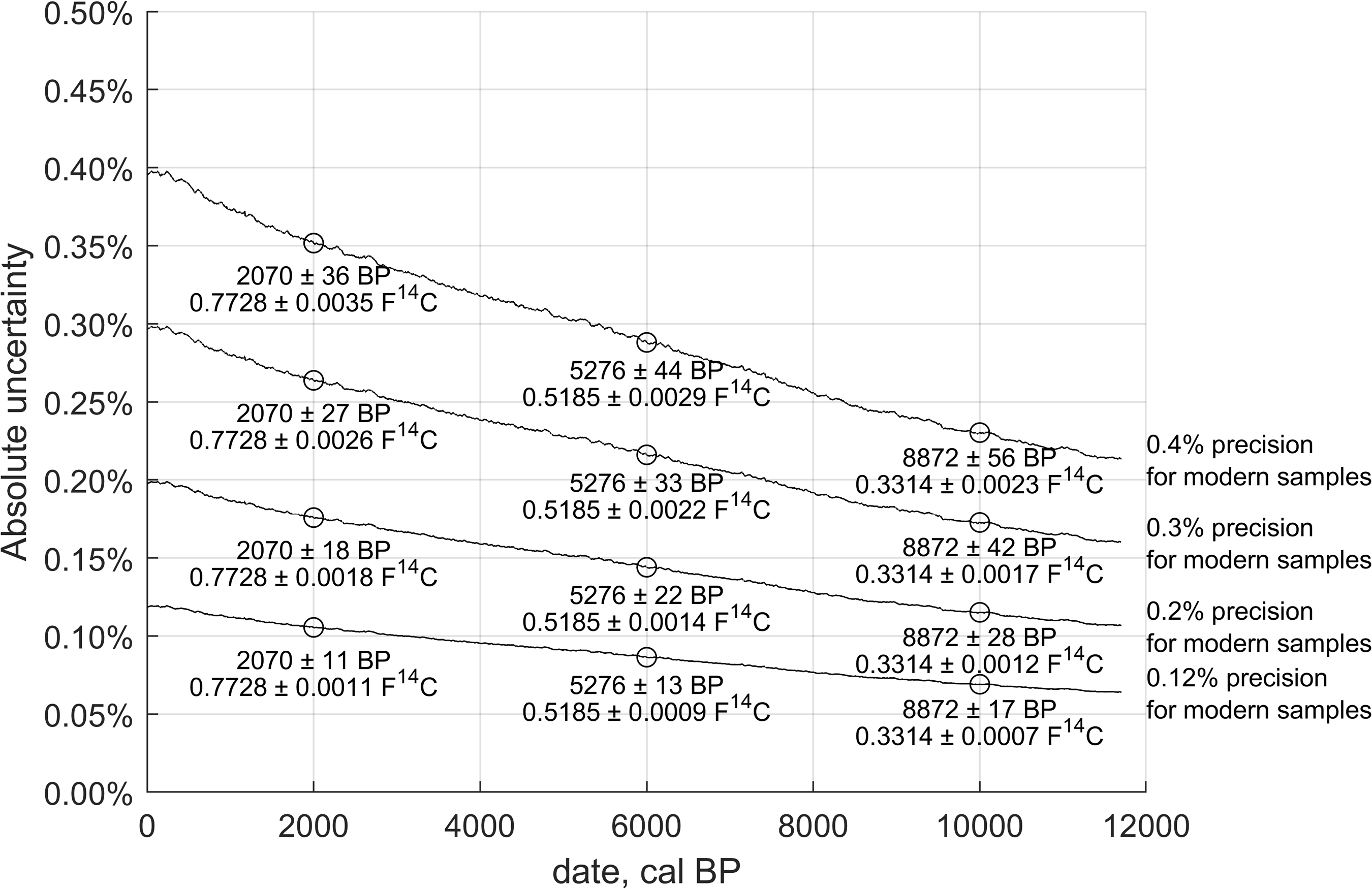
Figure 2A. Relation between absolute uncertainty of the measurement, for various levels of precision for modern samples.
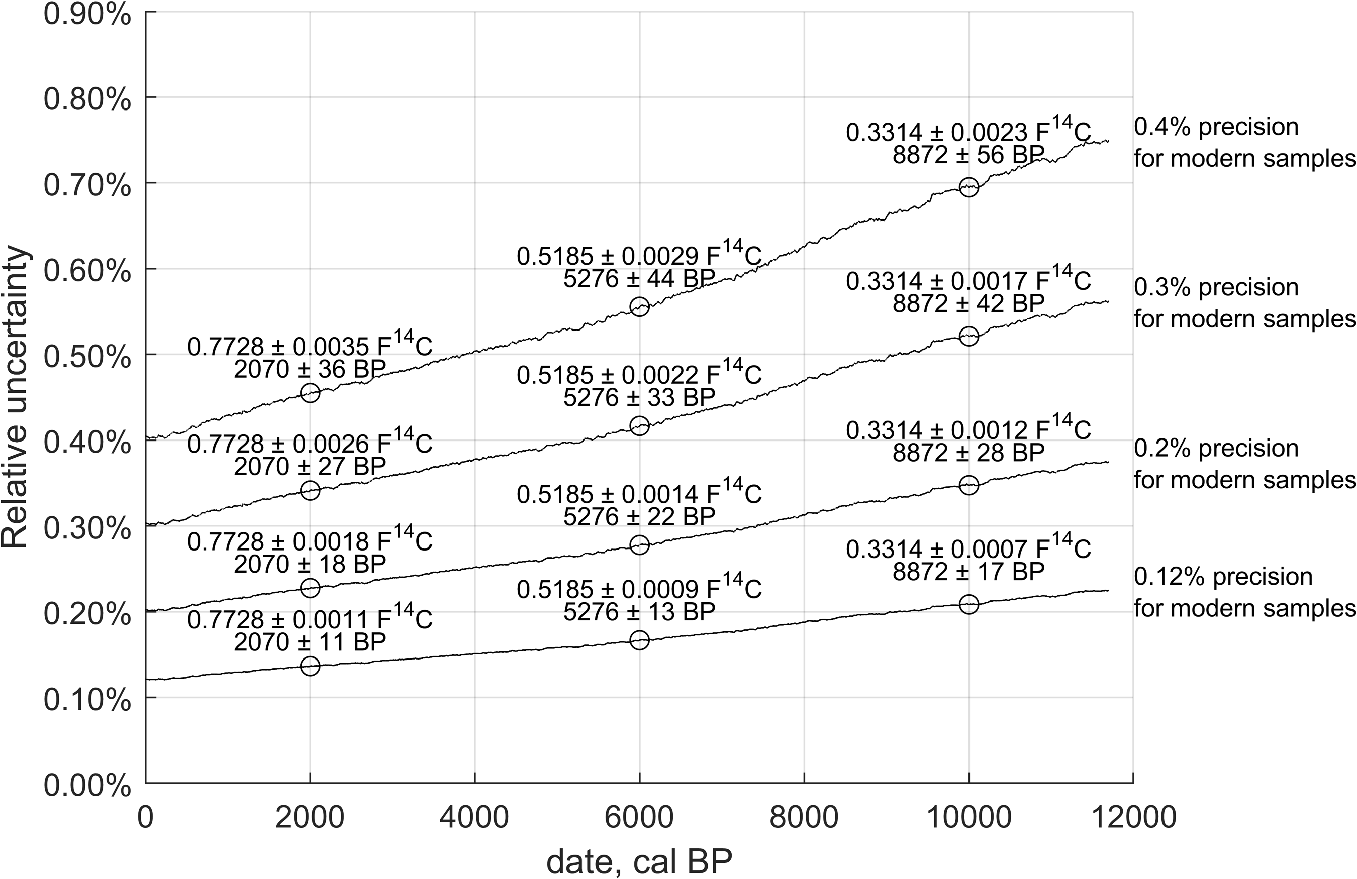
Figure 2B. Relation between relative uncertainty of the measurement, for various levels of precision for modern samples.
Calibration possibilities
A plot of cal BP ranges vs. calendar year is presented in Figures 3A and 3B for the Holocene. As expected, improved measurement precision leads to narrower cal BP ranges. However, due to fluctuations in atmospheric 14C concentrations, the same level of precision in 14C measurements can result in significantly different calibrated year spans (cal BP range). The cal BP ranges mirror the rapid fluctuations of the calibration curve and their variations are not related to the age of the samples.
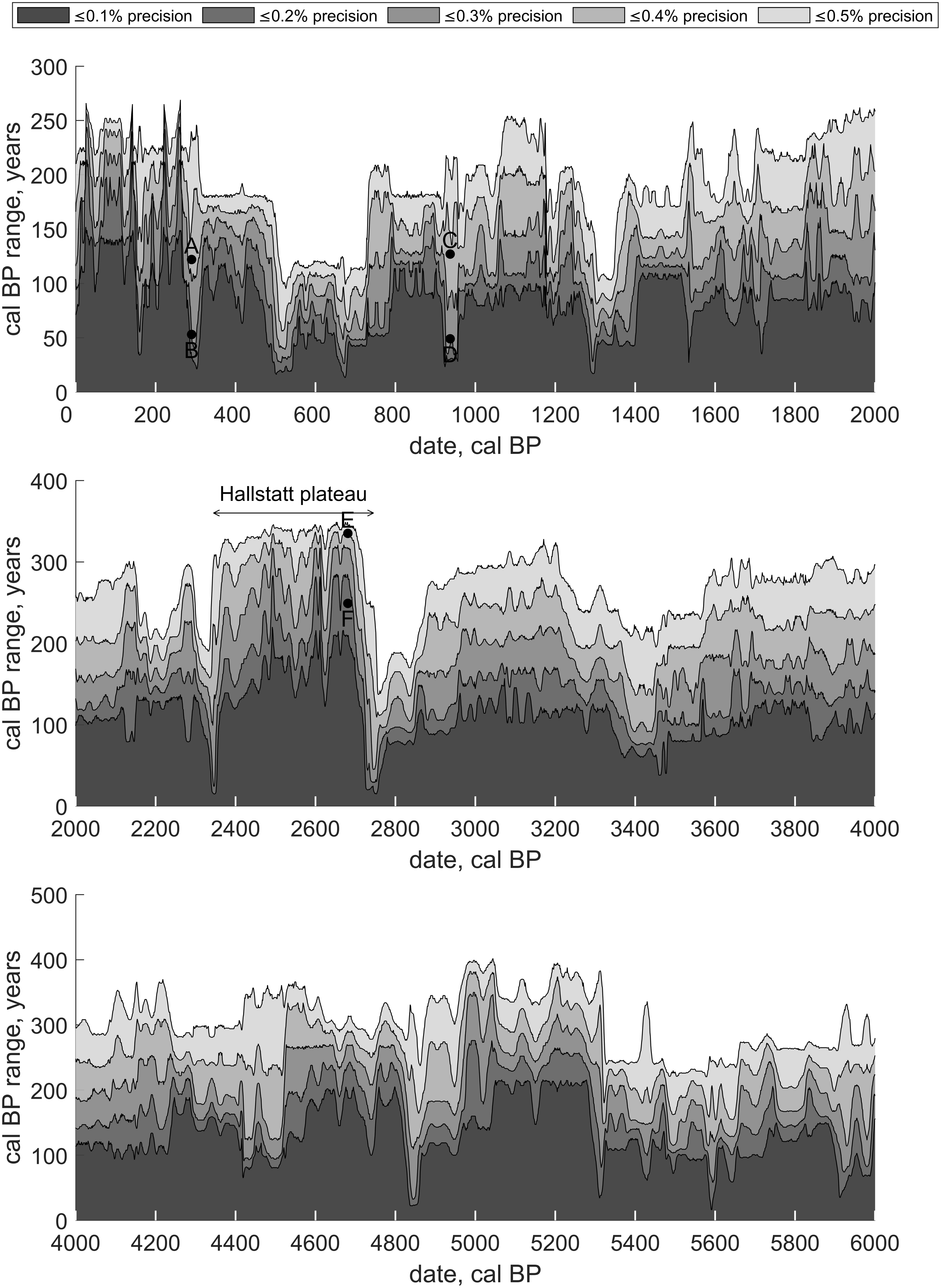
Figure 3A. The cal BP range vs. calendar year expressed in cal BP (years before AD 1950). The areas denote the ≤0.1%, ≤0.2%, ≤0.3%, ≤0.4%, ≤0.5%, measurement precision for modern samples, as described in the text.
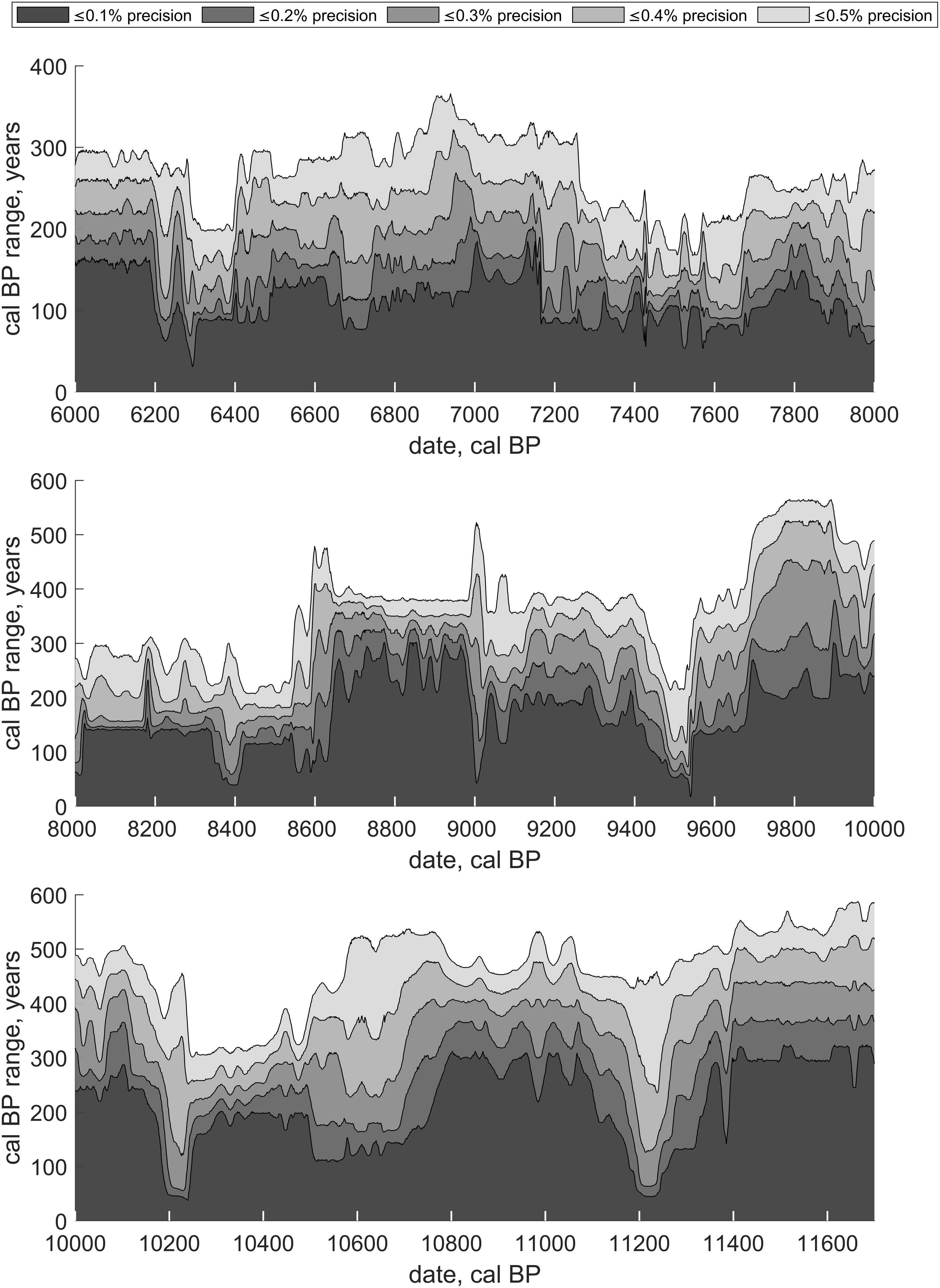
Figure 3B. The cal BP range vs. calendar year expressed in cal BP (years before AD 1950). The areas denote the ≤0.1%, ≤0.2%, ≤0.3%, ≤0.4%, ≤0.5%, measurement precision for modern samples, as described in the text.
During the Hallstatt plateau (2350–2750 cal BP), for example, 0.7359 ± 0.0034 F14C (point E in Figure 3A) yields a cal BP range of 337 years, while 0.7359 ± 0.0013 F14C (point F in Figure 3A) results in a 255-year cal BP range. Therefore, even a significant increase in measurement precision would not be beneficial for most applications of single-sample dating in this period.
On the other hand, for 0.8778 ± 0.0035 F14C, reducing the uncertainty to 0.8778 ± 0.0020 F14C narrows the cal BP range from 128 years to 50 years (points C and D in Figure 3A, respectively). This reduction of the uncertainty may be beneficial for some applications.
If single-sample dating is coupled with prior information, cal BP ranges below 30 years can be achieved. For 0.9724 ± 0.0018 F14C (point B in Figure 3A), two distinct intervals of 29 and 24 years are obtained, totaling a 53-year cal BP range. These intervals are separated by a 102-year calendar gap. If prior information is available for this period, one interval can be excluded, further narrowing the possible cal BP range. Conversely, for 0.9724 ± 0.0035 F14C (point A in Figure 3A), the two intervals expand to 49 and 74 years, with a smaller separating gap of 46 calendar years. At this precision level an additional third interval also appears, increasing the total cal BP range to 147 years.
As shown in Figures 3A and 3B, there are certain periods where high-precision measurement are especially beneficial such as around 10,200 cal BP and 11,200 cal BP. Therefore, Figures 3A and 3B may be used in planning the archaeological studies and can assist in evaluating whether high-precision radiocarbon dating is beneficial for the study.
During radiocarbon measurements, cal BP range vs. radiocarbon determination can be used to decide if a sample would benefit from longer measurement. Those graphs are available in the Supplementary Material (Figures S1 and S2).
By analyzing the probability distributions of cal BP ranges over longer periods (Figure 4), one finds that higher precision significantly reduces the mean cal BP ranges, as to be expected. In Figure 4, the Holocene epoch was arbitrarily divided into three stages for better clarity. For calendar years from 0 cal BP to 2000 cal BP, mean cal BP ranges are as follows: 93, 105, 118, 133, and 149 years for precisions of 0.15%, 0.20%, 0.25%, 0.30%, and 0.35%, respectively. From 2000 cal BP to 6000 cal BP, mean cal BP ranges are 139, 158, 178, 199, and 222 years are obtained at the same respective precision levels. Finally, between 6000 cal BP and 11,700 cal BP, mean cal BP ranges of 184, 208, 233, 258, and 285 years are observed at the corresponding precision levels for modern samples as described above.

Figure 4. Probability distribution of cal BP ranges for various levels of measurement precision for modern samples, as described in the text.
The IntCal20 calibration curve (Reimer et al. Reference Reimer, Austin, Bard, Bayliss, Blackwell, Bronk Ramsey, Butzin, Cheng, Edwards, Friedrich, Grootes, Guilderson, Hajdas, Heaton, Hogg, Hughen, Kromer, Manning, Muscheler, Palmer, Pearson, van der Plicht, Reimer, Richards, Scott, Southon, Turney, Wacker, Adolphi, Büntgen, Capano, Fahrni, Fogtmann-Schulz, Friedrich, Köhler, Kudsk, Miyake, Olsen, Reinig, Sakamoto, Sookdeo and Talamo2020) is significantly more detailed than preceding calibration curves, due to the incorporation of more annual data and the application of advanced mathematical methods (Heaton et al. Reference Heaton, Blaauw, Blackwell, Bronk Ramsey, Reimer and Scott2020). The new calibration curve tends to be less oversmoothed and follows more accurately the variations in atmospheric 14C levels (see Figure 4 in Reimer et al. Reference Reimer, Austin, Bard, Bayliss, Blackwell, Bronk Ramsey, Butzin, Cheng, Edwards, Friedrich, Grootes, Guilderson, Hajdas, Heaton, Hogg, Hughen, Kromer, Manning, Muscheler, Palmer, Pearson, van der Plicht, Reimer, Richards, Scott, Southon, Turney, Wacker, Adolphi, Büntgen, Capano, Fahrni, Fogtmann-Schulz, Friedrich, Köhler, Kudsk, Miyake, Olsen, Reinig, Sakamoto, Sookdeo and Talamo2020). The average number of distinct ranges for a single 14C date during the Holocene has increased since the IntCal13 from 2.13 per calendar year (Reimer et al. Reference Reimer, Bard, Bayliss, Beck, Blackwell, Ramsey, Buck, Cheng, Edwards, Friedrich, Grootes, Guilderson, Haflidason, Hajdas, Hatté, Heaton, Hoffmann, Hogg, Hughen, Kaiser, Kromer, Manning, Niu, Reimer, Richards, Scott, Southon, Staff, Turney and van der Plicht2013), to 2.36 per calendar year with IntCal20 (Reimer et al. Reference Reimer, Austin, Bard, Bayliss, Blackwell, Bronk Ramsey, Butzin, Cheng, Edwards, Friedrich, Grootes, Guilderson, Hajdas, Heaton, Hogg, Hughen, Kromer, Manning, Muscheler, Palmer, Pearson, van der Plicht, Reimer, Richards, Scott, Southon, Turney, Wacker, Adolphi, Büntgen, Capano, Fahrni, Fogtmann-Schulz, Friedrich, Köhler, Kudsk, Miyake, Olsen, Reinig, Sakamoto, Sookdeo and Talamo2020), assuming a measurement precision of 0.2% for modern samples. The statistical increase of the presence of multiple intervals during calibration is generally advantageous, as any available prior information (e.g. stratigraphical, historical, contextual) may significantly narrow the calibrated range of calendar year determination.
Conclusion
Understanding the relationship between the raw radiocarbon measurement (along with its associated uncertainty) and the calibrated age range is crucial in radiocarbon dating. The calibrated age range (cal BP range) based on a single radiocarbon date may exceed 200 years (at the 95.4% probability), within the Holocene epoch, even for a high-precision measurements. However, there are instances on the calibration curve where a range of less than 50 years is achievable, making high-precision measurements highly beneficial. These calibration and measurement limitations are critical when high-precision results are required for a single radiocarbon date. As has been demonstrated, we believe that effective communication between archaeologists or earth scientists and radiocarbon experts allows for the selection of the precision needed depending on the site context, and Figures 3A and 3B may be helpful in this communication.
Supplementary material
To view supplementary material for this article, please visit https://doi.org/10.1017/RDC.2025.26
Acknowledgments
Publication supported by the Excellence Initiative – Research University program implemented at the Silesian University of Technology, year 2024, and by the NCN grant no. UMO-2020/37/B/HS3/01622, Chronology of the Inca expansion in the Cordillera de Vilcabamba (Peru). The open access publication fee is covered by project no. FESL.10.25-IZ.01-06C9/23-00 from EU funds FSD – 10.25 Development of higher education focused on the needs of the green economy European Funds for Silesia 2021–2027: The modern methods of the monitoring of the level and isotopic composition of atmospheric CO2.


 Open access