


INTRODUCTION
Cosmogenic radionuclide inventories in fluvial and alluvial sediments reflect the sediment flux out of the catchment area and have been used to estimate basin-average erosion rates for more than 25 years (Brown et al. Reference Brown, Stallard, Larsen, Raisbeck and Yiou1995; Bierman and Steig Reference Bierman and Steig1996; Granger et al. Reference Granger, Kirchner and Finkel1996; Portenga and Bierman Reference Portenga and Bierman2011). Calculating an erosion rate or an exposure age requires the cosmogenic radionuclide production rate, which is specific to the site (latitude, longitude, and elevation above sea level). Near the Earth’s surface, production of in situ cosmogenic 10Be and 26Al is dominated by high-energy spallation; at depth production by negative muon capture and fast muon interaction becomes significant. Site-specific production rates are calculated using one of several published scaling methods (Lal Reference Lal1991; Stone Reference Stone2000; Dunai Reference Dunai2001; Lifton et al. Reference Lifton, Smart and Shea2008; Desilets et al. Reference Desilets, Zreda and Prabu2006; Lifton et al. Reference Lifton, Sato and Dunai2014) and a sea-level and high-latitude reference production rate (e.g., Borchers et al. Reference Borchers, Marrero, Balco, Caffee, Goehring, Lifton, Nishiizumi, Phillips, Schaefer and Stone2016; Martin et al. Reference Martin, Blard, Balco, Lavé, Delunel, Lifton and Laurent2017). The calculation of a site-specific production rate also depends on the choice of an atmospheric model to convert elevation to atmospheric depth, a palaeomagnetic framework to account for the effects of the Earth’s magnetic field on the cosmic-ray flux, the attenuation length in rock and the choice of a model of muogenic nuclide production. Online calculators (Balco et al. Reference Balco, Stone, Lifton and Dunai2008; Marrero et al. Reference Marrero, Phillips, Borchers, Lifton, Aumer and Balco2016; Martin et al. Reference Martin, Blard, Balco, Lavé, Delunel, Lifton and Laurent2017) harmonize these calculations and have greatly improved the reproducibility of cosmogenic nuclide exposure ages and erosion rates.
Cosmogenic nuclide concentrations in river sediments provide a spatially averaged signal of the rates at which the catchment is eroding and can be used to quantify erosion processes within landscapes (Bierman and Steig Reference Bierman and Steig1996). The calculation of catchment-averaged erosion rates assumes that erosion rates are constant, that the catchment area is in isotopic steady state, and that the sediment is well mixed and sediment storage within the basin is negligible (e.g., von Blanckenburg Reference von Blanckenburg2005). Because production rates are site-specific, the calculation of catchmentwide erosion rates depends on the complete production rate model of the basin. For settings with little variability in production rates, a single “basin-wide” production rate determined from the basin mean latitude, longitude and elevation may provide a good approximation of the catchmentwide erosion rate (Brown et al. Reference Brown, Stallard, Larsen, Raisbeck and Yiou1995). More advanced approaches are based on spatially resolved production rates determined from a pixel array that represents the catchment topography (e.g., Belmont et al. Reference Belmont, Pazzaglia and Gosse2007; Portenga and Biermann Reference Portenga and Bierman2011; Lupker et al. Reference Lupker, Blard, Lavé, France-Lanord, Leanni, Puchol, Charreau and Bourlès2012; Godard et al. Reference Godard, Bourlès, Spinabella, Burbank, Bookhagen, Fisher, Moulin and Léanni2014; Scherler et al. Reference Scherler, Bookhagen and Strecker2014). For computational efficiency these calculations are often based on the time-constant production rate scaling of Lal (Reference Lal1991)/Stone (Reference Stone2000), which does not account for variations in the Earth’s magnetic field, although solutions that incorporate a geomagnetic correction after Nishiizumi et al. (Reference Nishiizumi, Winterer, Kohl, Klein, Middleton, Lal and Arnold1989) have been developed (Scherler et al. Reference Scherler, Bookhagen and Strecker2014; Charreau et al Reference Charreau, Blard, Zumaque, Martin, Delobel and Szafran2019).
Previously published algorithms for calculating catchmentwide erosion rates (Mudd et al. Reference Mudd, Harel, Hurst, Grieve and Marrero2016; Charreau et al. Reference Charreau, Blard, Zumaque, Martin, Delobel and Szafran2019) are independent of existing online calculators (Balco et al. Reference Balco, Stone, Lifton and Dunai2008; Marrero et al. Reference Marrero, Phillips, Borchers, Lifton, Aumer and Balco2016; Martin et al. Reference Martin, Blard, Balco, Lavé, Delunel, Lifton and Laurent2017), even if the calculations are based on the same scaling methods as those implemented in the online calculators. Catchmentwide erosion rates determined in this way are therefore not fully comparable to exposure ages and point-based erosion rates calculated with the existing calculators, although in practice the discrepancies may be small compared to the uncertainties arising from the assumptions that are made when a basin-average erosion rate is determined from a river sediment sample (e.g., von Blanckenburg Reference von Blanckenburg2005). We introduce “riversand”, a new python package for the efficient computation of catchmentwide erosion rates fully integrated with the existing online exposure age and erosion rate calculator provided and maintained by G. Balco (Balco et al. Reference Balco, Stone, Lifton and Dunai2008), (http://hess.ess.washington.edu, http://stoneage.ice-d.org, or http://stoneage.hzdr.de). The package is published in the Python Package Index repository (https://pypi.org/project/riversand/) and includes an installation guide and example scripts. It is a key feature of riversand that all future updates to the production rate calculation of the online calculator are immediately effective for the calculation of catchmentwide erosion rates and that the results are therefore fully comparable and future-proof. This contribution provides a description of the riversand calculator and an illustrative comparison to erosion rates calculated with the Basinga cell-by-cell GIS toolbox (Charreau et al. Reference Charreau, Blard, Zumaque, Martin, Delobel and Szafran2019) and the CAIRN method (Mudd et al. Reference Mudd, Harel, Hurst, Grieve and Marrero2016).
PRINCIPLES
Every location within a catchment has its unique (time-dependent) production rate, which for a given erosion rate can be expressed as a function of the geographic coordinates (latitude and longitude) and the elevation above sea level. Note that we use the term “erosion” instead of “denudation” to refer to the removal of mass from the Earth’s surface without the distinction between physical erosion and chemical weathering to keep in line with the usage of “erosion” in the online calculator. In practice, production rates are much more sensitive to changes in elevation than latitude (Lal Reference Lal1991). Following the approach of Bierman and Steig (Reference Bierman and Steig1996), we use the catchment hypsometry to subdivide the catchment into regions of similar elevation with a representative nuclide production rate P i for each subregion i (Figure 1a, b).
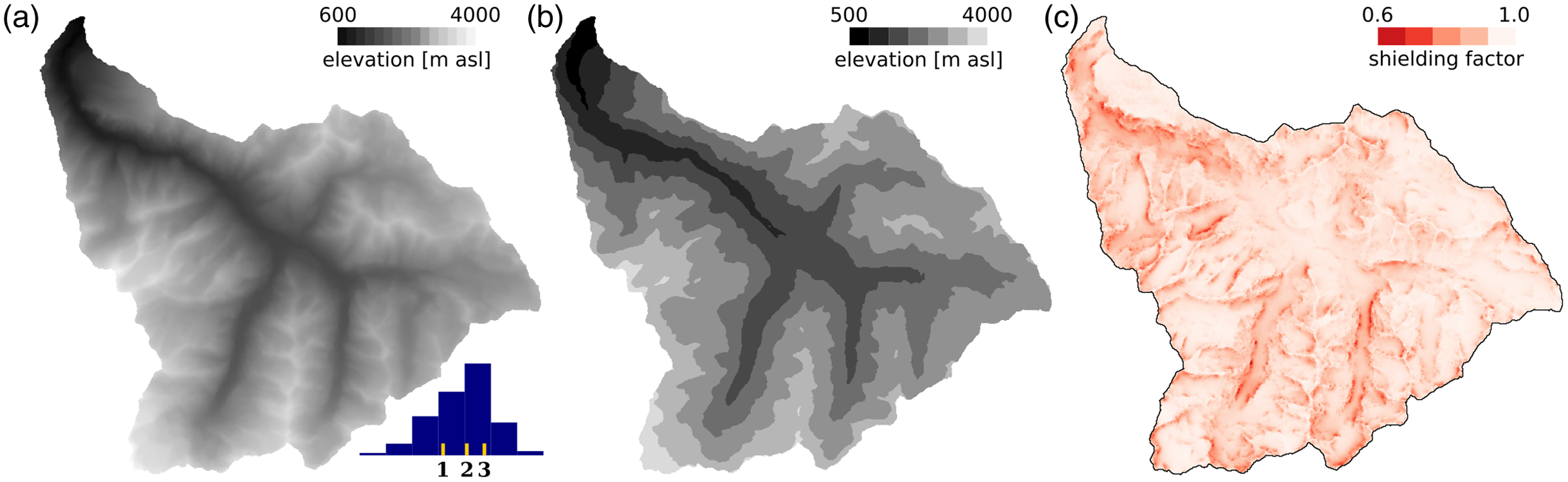
Figure 1 Example catchment, area 257 km2, elevations 640 to 4020 m asl. (a) Topography from a NASADEM digital elevation model, projected to UTM 32N, pixel resolution 35 m (NASA JPL 2021). Inset shows a histogram of elevations with a bin size of 500 m; quartiles (1: 2082, 2: 2532, 3: 2850 m asl) are indicated. (b) Catchment topography binned with a bin size of 500 m, i.e., subdivided into seven subregions. (c) Topographic shielding raster dataset calculated from the same elevation model using the toposhielding function of TopoToolbox (Schwanghart and Scherler Reference Schwanghart and Scherler2014).
For time-constant production rates after Lal/Stone the production rate of the entire catchment may be calculated as an area-weighted average of the production rates of the subregions. For the more general case of a time-dependent production rate model, the cosmogenic nuclide production of each subregion N pred,i (E) is calculated by the online calculator for a given erosion rate E based on the mean elevation of the subregion i and the centroid coordinates of the entire catchment (Figures 2 and 3). The calculation of N pred,i (E) by the online calculator is described in Balco et al. (Reference Balco, Stone, Lifton and Dunai2008; their Eq. 2). Shielding factors (e.g., topographic shielding, snow shielding, or vegetation shielding) may be assumed constant for the entire catchment. Alternatively, if spatially resolved shielding factors are available, a mean shielding factor is determined for each subregion i of the elevation-binned catchment and included in the calculation of N pred,i (E) (Figure 1c). The predicted nuclide concentration at the catchment outlet for the given erosion rate E is the sum of predicted nuclide concentrations of each subregion N pred,i (E) normalized by the area of the subregion A i :
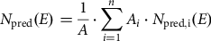 $${N_{\rm pred}}(E) = {1 \over A} \cdot \sum\limits_{i = 1}^n {{A_i} \cdot {N_{\rm pred,i}}(E)} $$
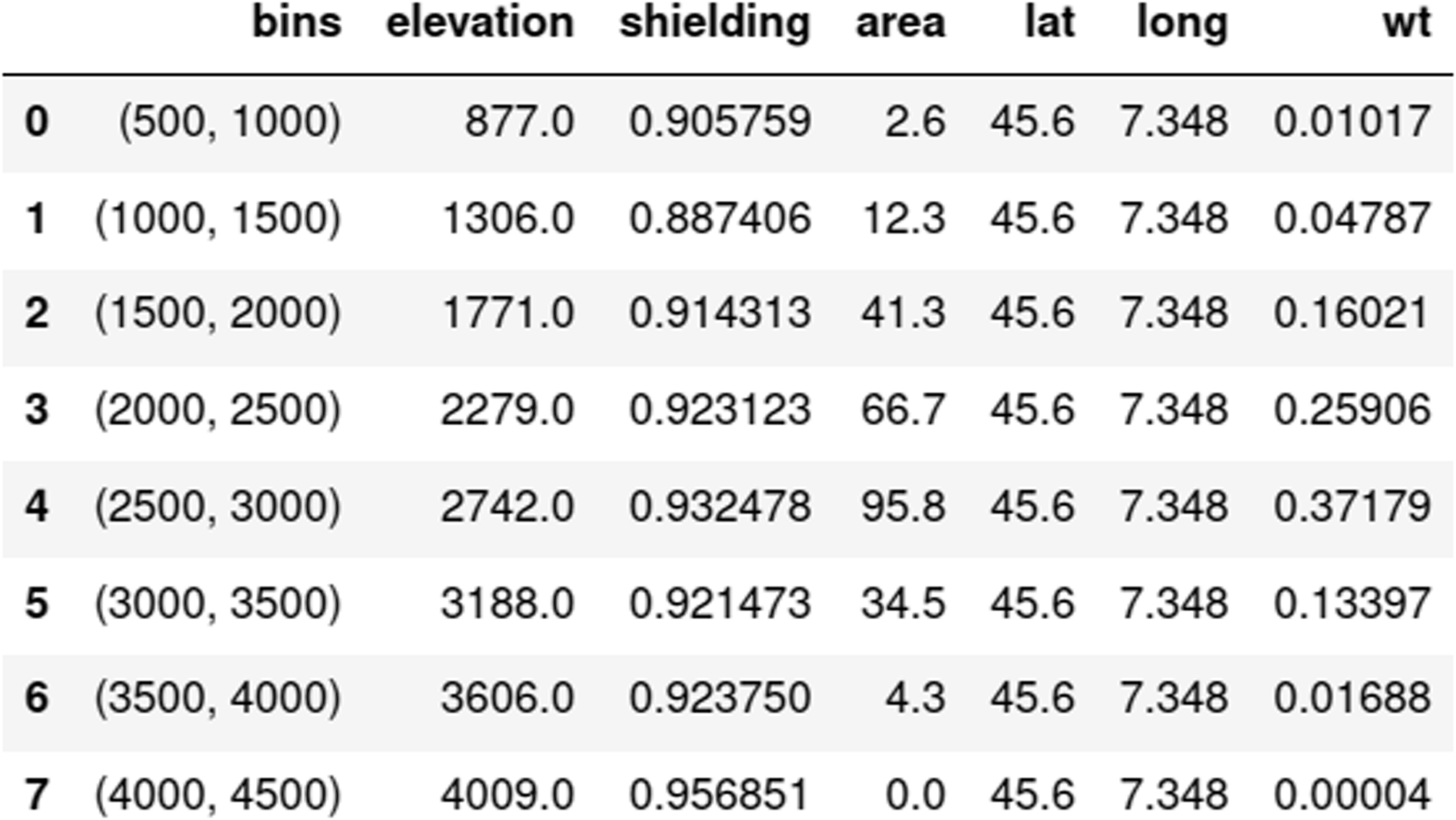
Figure 2 “Riversand” output: hypsometry statistics (bin size 500 m) used for the prediction of nuclide production in the catchment: “elevation” and “area” are the mean elevation and the area in km2 of each subregion, “wt” is the nomalized area. “lat” and “long” are the centroid coordinates of the catchment. In this example, a mean shielding factor “shielding” was calculated for each subregion i from a topographic shielding raster (Figure 1c).
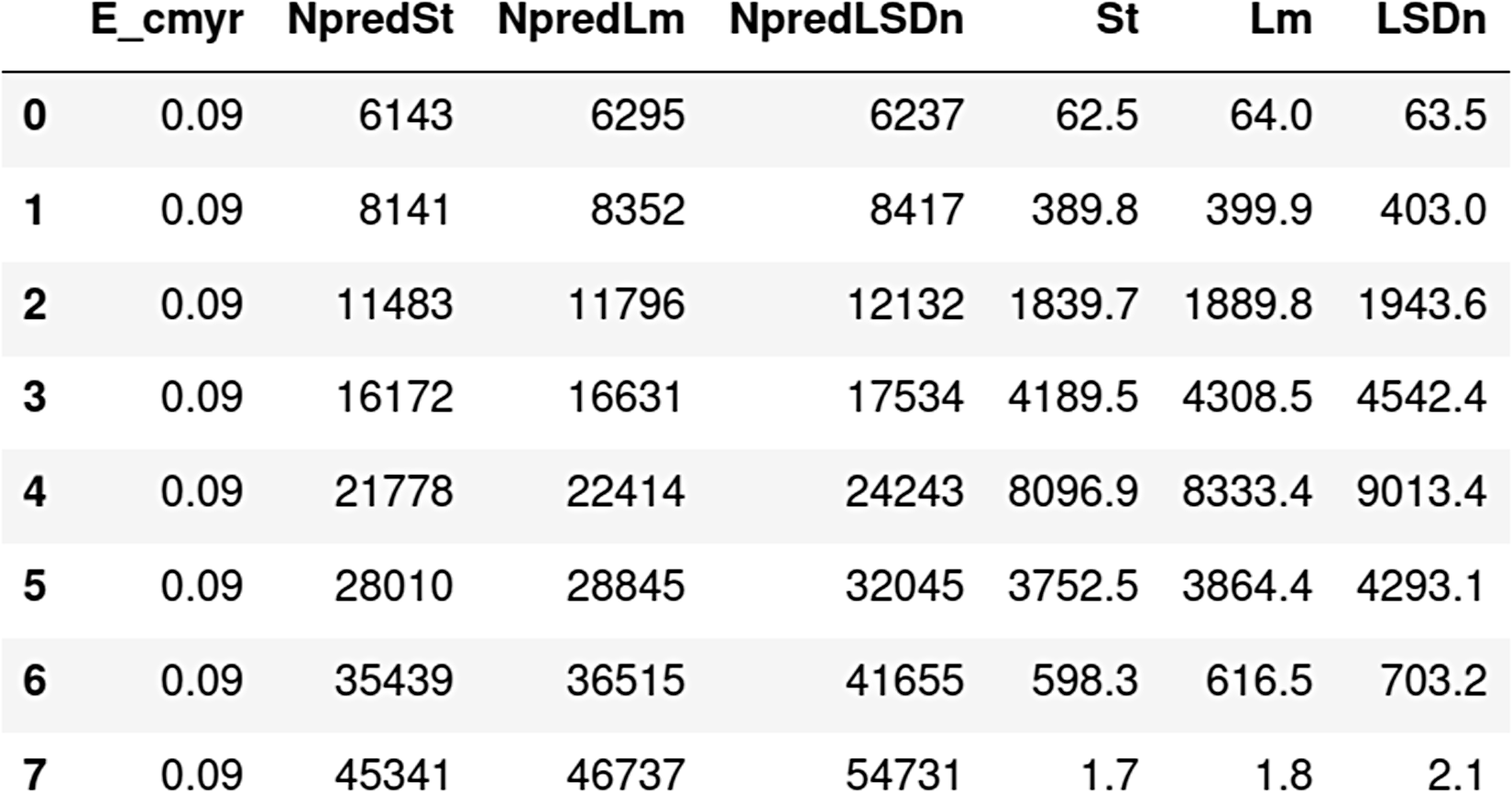
Figure 3 “Riversand” output: Predicted nuclide concentrations “NpredSt”, “NpredLm”, “NpredLSDn” for each subregion of the catchment determined from the hypsometry statistics (Figure 2) for an erosion rate of 0.09 cm/yr for the three scaling methods currently implemented in the online calculator (St: time-independent Lal Reference Lal1991/Stone Reference Stone2000; Lm: time-dependent version of St; LSDn: time-dependent after Lifton et al. Reference Lifton, Sato and Dunai2014). “St”, “Lm”, “LSDn” are the predicted nuclide concentrations normalized by the area of each subregion (“wt” in Figure 2).
To calculate the catchmentwide erosion rate E that corresponds to the measured nuclide concentration at the catchment outlet N meas, we use the online calculator to predict nuclide concentrations for a suite of different erosion rates E n and fit a polynomial function of the form y = a/x2+b/x+c to these data (Figure 4). The uncertainty in E, delE, is determined from the uncertainty in the measured nuclide concentration, delN meas, and the empirical polynomial function; it does not include the uncertainties in the production rate estimates. delE is asymmetric and generally smaller for high nuclide concentrations or low erosion rates.
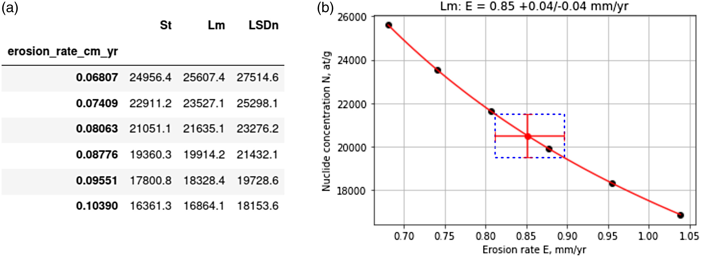
Figure 4 “Riversand” output: (a) Predicted nuclide concentrations at the catchment outlet for three different scaling methods “St”, “Lm”, “LSDn” and for six different erosion rates. (b) Predicted nuclide concentrations as a function of erosion rate for “Lm” scaling. The catchmentwide erosion rate E corresponding to the measured nuclide concentration at the catchment outlet, N meas, is determined from the polynomial function y = a/x2+b/x+c fit to the data points (red line and point). The uncertainty in E, delE, is determined from the uncertainty in the measured nuclide concentration, delN meas, and the empirical polynomial function (red error bars and dashed line). (Please see online version for color figures.)
Although the catchmentwide erosion rate E may be determined iteratively from an arbitrary set of initial erosion rates E n , an efficient computation of E is achieved with a suitable set of initial values. We estimate the bracket of initial erosion rates, E min and E max , from the first and third quartile of the catchment hypsometry (Figure 1a, inset); the computation of E min and E max is performed by the online calculator. By default the initial erosion rates are six values that are logarithmically distributed from E min to E max (Figure 4).
The scaling methods available in the riversand calculator are those that are implemented in the online calculator and described in Balco et al. (Reference Balco, Stone, Lifton and Dunai2008) and the online documentation at http://stoneage.ice-d.org/; currently these are “St”: a time-constant scaling method after Lal (Reference Lal1991) and Stone (Reference Stone2000); “Lm”: a time-dependent version of the Lal/Stone method that incorporates magnetic field fluctuations and solar modulation after Nishiizumi et al. (Reference Nishiizumi, Winterer, Kohl, Klein, Middleton, Lal and Arnold1989); and “LSDn”: a time-dependent and nuclide-specific scaling method after Lifton et al. (Reference Lifton, Sato and Dunai2014), which is also favoured by the CRONUScalc online calculator (Marrero et al. Reference Marrero, Phillips, Borchers, Lifton, Aumer and Balco2016). Geomagnetic corrections for Lm and LSDn scaling are based on a composite geocentric/axial dipole field reconstruction (DGRF/SHA.DIF14k/GLOPAD models; Lifton Reference Lifton2016). Atmospheric scaling is based on the ERA-40 reanalysis (Uppala et al. Reference Uppala, Kållberg, Simmons, Andrae, da Costa Bechtold, Fiorino, Gibson, Haseler, Hernandez and Kelly2005); the Stone/Radok atmospheric model (Radok et al. Reference Radok, Allison and Wendler1996; Stone Reference Stone2000) is also implemented and is recommended for sites in Antarctica. Muogenic production is approximated by a single erosion-rate dependent exponential (Balco et al. Reference Balco, Stone, Lifton and Dunai2008; Balco Reference Balco2017). Reference production rates are sourced from the CRONUS-Earth primary data set (http://calibration.ice-d.org/ accessed 2016-12-04).
Input data for the riversand calculator are (1) a digital elevation model of the study area in an equal-area projection in geotiff format (“elevation raster”; for example, NASA JPL (2021) NASADEM); (2) the catchment outline(s) as polygon shapefile; (3) a spreadsheet with sample and nuclide data corresponding to the input of the online calculator. In addition, there are two optional input datasets: (1) shielding data may be provided as a constant value for each catchment or as a shielding raster dataset; for example, topographic shielding may be calculated from the elevation raster using the toposhielding function of the TopoToolbox (Schwanghart and Scherler Reference Schwanghart and Scherler2014) and included in the calculation, and (2) a raster dataset that classifies the catchment into “quartz-bearing” and “quartz-free” lithologies may be used to exclude the quartz-free portions of the catchment from the calculation (Delunel et al. Reference Delunel, Van Der Beek, Carcaillet, Bourlès and Valla2010). The calculator has options to process a single catchment or multiple catchments. The workflow to using the riversand calculator comprises two steps: (1) import and validate all input data, and (2) process the catchments by calling a single function that performs the calculations outlined above with specified parameters such as bin size for the catchment hypsometry and scaling method. The output includes catchmentwide erosion rates calculated with the available scaling methods (St, Lm, LSDn) as well as some catchment statistics (e.g., catchment area and mean elevation) and can be saved as a csv-file or an Excel spreadsheet. The calculator also saves images of the clipped catchments, the elevation histograms and the empirical function N pred (E) (see Figure 4b).
The riversand calculator communicates with the online calculator via a URL request. The performance depends on the number of values N pred that need to be calculated by the online calculator. In particular, the computation will become slow or may fail if a very small elevation bin size is selected, i.e., if the table of hypsometry statistics (see Figure 2) becomes very large. We recommend a bin size of 100 m for standard applications. On the other hand, the size or resolution of the catchment elevation model has little impact on computation times, and there is no need to resample the elevation model of a large catchment to a low resolution. The computation time for a single catchment is typically <30 seconds independent of the (time-constant or time-dependent) scaling method.
EXAMPLES
To illustrate the use of the riversand calculator, we recalculated catchmentwide erosion rates published in two recent studies from the Western Alps (Serra et al. Reference Serra, Valla, Delunel, Gribenski, Christl and Akçar2022) and the Peruvian Andes (Reber et al. Reference Reber, Delunel, Schlunegger, Litty, Madella, Akçar and Christl2017), respectively. Both study areas are from high-relief terrain where the effects of catchment hypsometry on production rates are expected to be most pronounced. Catchment sizes are 50–3300 km² (Western Alps) and 600–17000 km² (Peruvian Andes). Published erosion rates are 300 to 1500 mm/kyr in the Western Alps (Serra et al. Reference Serra, Valla, Delunel, Gribenski, Christl and Akçar2022; calculated with Basinga, Charreau et al. Reference Charreau, Blard, Zumaque, Martin, Delobel and Szafran2019) and 9–240 mm/kyr in the Peruvian Andes (Reber et al. Reference Reber, Delunel, Schlunegger, Litty, Madella, Akçar and Christl2017; calculated with CAIRN, Mudd et al. Reference Mudd, Harel, Hurst, Grieve and Marrero2016).
High-Relief Catchments in the Western Alps
Serra et al. (Reference Serra, Valla, Delunel, Gribenski, Christl and Akçar2022) present 10Be concentrations from 19 fluvial sediment samples in the Dora Baltea catchment in the Western Alps. Catchments are located 6.8 to 8.0°E and 45.4 to 46.0°N; catchment areas range from 54 to 3320 km² with topographic relief 2400 to 4500 m and catchment mean elevation 2000 to 2500 m asl. The terrain is partly glaciated, and steep headwalls and deeply incised valleys cause significant topographic shielding. Reported 10Be concentrations range from 1.08×10⁴ to 4.85×10⁴ atoms/grams quartz with analytical uncertainties typically 3 to 9% (Serra et al. Reference Serra, Valla, Delunel, Gribenski, Christl and Akçar2022). Catchmentwide erosion rates were calculated with Basinga (Charreau et al. Reference Charreau, Blard, Zumaque, Martin, Delobel and Szafran2019) using the Lal/Stone production rate scaling method (Lal Reference Lal1991; Stone Reference Stone2000) combined with the ERA-40 reanalysis database (Uppala et al. Reference Uppala, Kållberg, Simmons, Andrae, da Costa Bechtold, Fiorino, Gibson, Haseler, Hernandez and Kelly2005) and the VDM database (Muscheler et al. Reference Muscheler, Beer, Kubik and Synal2005) for atmospheric and geomagnetic correction, respectively. Sea-level high-latitude reference production rate is 4.18±0.26 at/g/yr with a relative contribution of fast and negative muons of 0.27% and 0.87%, respectively (Charreau et al. Reference Charreau, Blard, Zumaque, Martin, Delobel and Szafran2019 after Braucher et al. Reference Braucher, Merchel, Borgomano and Bourlès2011 and Martin et al. Reference Martin, Blard, Balco, Lavé, Delunel, Lifton and Laurent2017). Erosion rates are corrected for topographic shielding using the toposhielding function of TopoToolbox (Schwanghart and Scherler Reference Schwanghart and Scherler2014).
We compare the published results to erosion rates recalculated with the riversand calculator using the Lal/Stone (St), the modified time-dependent Lal/Stone (Lm) and the Lifton/Sato/Dunai (LSDn) scaling methods of the online calculator v.3 (Figure 5a). The most notable differences of the Lm scaling compared to the Lal/Stone scaling used in Serra et al. (Reference Serra, Valla, Delunel, Gribenski, Christl and Akçar2022) are: (1) a different framework for geomagnetic corrections; (2) a different 10Be reference spallation production (riversand: 4.208±0.316 at/g/yr vs. Basinga: 4.18±0.26 at/g/yr); (3) a different muogenic production model. Both calculations use an attenuation length of spallation production of 160 g/cm² and a rock density of 2.7 g/cm3. The riversand recalculation is based on the NASADEM digital elevation model (NASA JPL 2021) resampled to a resolution of 35 m and an elevation histogram with a bin size of 100 m.
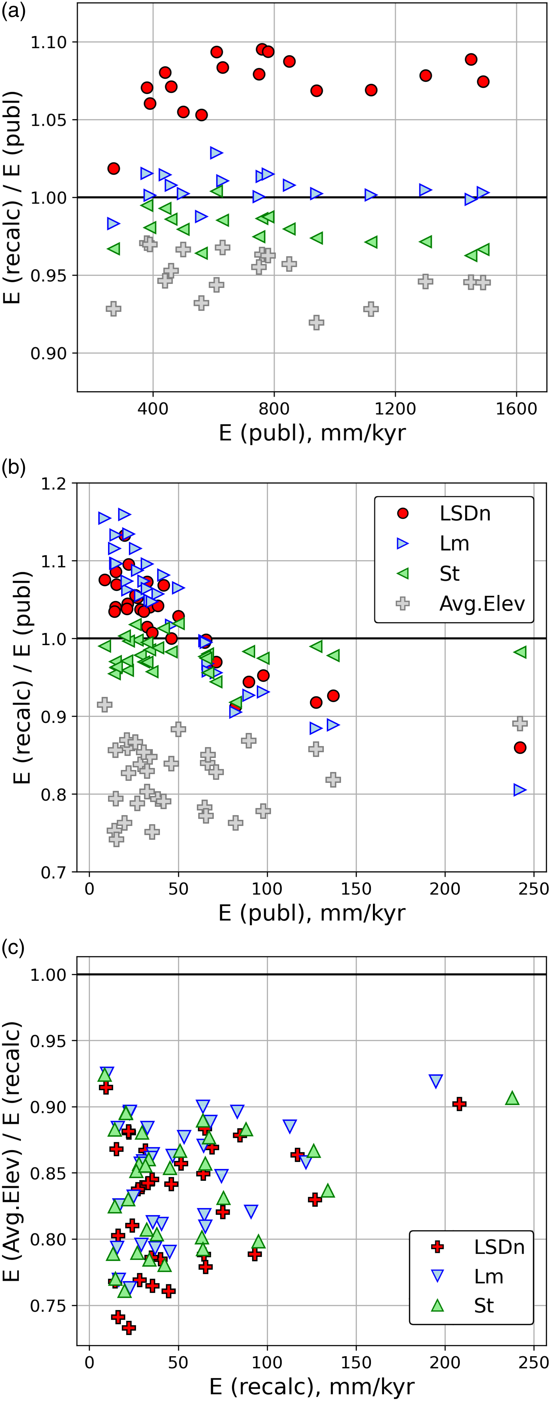
Figure 5 (a) Ratio of recalculated to published erosion rates for the Dora Baltea catchment, Western Alps (Serra et al. Reference Serra, Valla, Delunel, Gribenski, Christl and Akçar2022) for St: Lal/Stone, Lm: modified Lal/Stone, LSDn: Lifton/Seto/Dunai scaling (see (b) for legend). Grey crosses show erosion rates calculated from the catchment mean elevation instead of the catchment hypsometry (Lm scaling). The Lm scaling (blue triangles) corresponds approximately to the modified Lal/Stone scaling method used in the original publication. (b) Same as (a) for the Peruvian Andes (Reber et al. Reference Reber, Delunel, Schlunegger, Litty, Madella, Akçar and Christl2017). Catchment mean-elevation erosion rates (grey crosses) are based on St scaling. The St scaling (green triangles) corresponds approximately to the Lal/Stone scaling method used in the original publication. (c) Ratio of erosion rates approximated from the catchment mean elevation (E(Avg. Elev)) to the results of the complete production model (E(recalc)) for the data set of Reber et al. (Reference Reber, Delunel, Schlunegger, Litty, Madella, Akçar and Christl2017).
The differences between recalculated Lm erosion rates and the published values are mostly <2% (Figure 5a); this is within the rounding error, as the values are published to two significant figures. LSDn scaling yields 5–10% higher values, consistent with the results of a sensitivity analysis for similar latitudes and elevations by Charreau et al. (Reference Charreau, Blard, Zumaque, Martin, Delobel and Szafran2019; their Figure 1), even though these authors ascertain that for many natural cases the difference between Lal/Stone and Lifton/Sato/Dunai scaling is small. St scaling yields values ≤4% lower than the published rates. The uncertainties on the erosion rates include the analytical uncertainties in measured 10Be concentrations and production rate uncertainties (Charreau et al. Reference Charreau, Blard, Zumaque, Martin, Delobel and Szafran2019) and the function N pred (E) (this study), respectively; predicted uncertainties are similar for the published and the recalculated values (Supplementary Table S1).
In low-relief terrain with only minor variation in production rates, catchmentwide erosion rates may be approximated using a single production rate calculated from the mean elevation of the catchment (Brown et al. Reference Brown, Stallard, Larsen, Raisbeck and Yiou1995; Blanckenburg Reference von Blanckenburg2005). Figure 5a also shows erosion rates calculated from the centroid coordinates, mean elevation and mean topographic shielding of each catchment (Lm scaling). Because production varies approximately exponentially with elevation this approach generally underestimates the true erosion rates. In the present example, the results of this approach are ∼2–8% lower than values calculated from a complete production rate model of the catchment.
Large Catchments in the Peruvian Andes
Reber et al. (Reference Reber, Delunel, Schlunegger, Litty, Madella, Akçar and Christl2017) report 10Be concentrations from 42 fluvial sediment samples along the Pacific coast between 6°S and 20°S latitude. Catchment areas are >700 km² with several catchments >10000 km². Peak elevations are >6000 m asl. Reported 10Be concentrations range from 8.5×10⁴ to 1.0×10⁶ atoms/grams quartz with analytical uncertainties ∼3% (Reber et al. Reference Reber, Delunel, Schlunegger, Litty, Madella, Akçar and Christl2017). Catchmentwide erosion rates were calculated with CAIRN (Mudd et al. Reference Mudd, Harel, Hurst, Grieve and Marrero2016) with the default parameters of the program and a rock density of 2.65 g/cm³. CAIRN uses the time-constant Lal/Stone scaling method and the NCEP2 climate reanalysis data (Compo et al. Reference Compo, Whitaker, Sardeshmukh, Matsui, Allan, Yin, Gleason, Vose, Rutledge and Bessemoulin2011) for atmospheric scaling. The sea-level high-latitude reference production rate is 4.30±0.39 at/g/yr. Muogenic production is modelled as the sum of two exponential functions for fast and negative muons, respectively. Similar to Basinga (Charreau et al. Reference Charreau, Blard, Zumaque, Martin, Delobel and Szafran2019) and the current version of the online calculator, the spallation attenuation length is 160 g/cm². Topographic shielding is calculated as part of the CAIRN algorithm and follows the method of Codilean (Reference Codilean2006).
Because of the large size of the study area and the large catchment areas, Reber et al. (Reference Reber, Delunel, Schlunegger, Litty, Madella, Akçar and Christl2017) use a 200-m resolution digital elevation model for the pixel-based calculation of catchmentwide erosion rates (resampled from a 90-m resolution SRTM digital elevation model, Jarvis et al. Reference Jarvis, Reuter, Nelson and Guevara2008). We recalculated erosion rates using a 100-m resolution NASADEM (NASA JPL 2021) and elevation histograms with a bin size of 100 m. Figure 5b compares recalculated rates (St, Lm and LSDn scaling) to published values. The St results are similar to (∼0–5% lower than) published rates. Although Mudd et al. (Reference Mudd, Harel, Hurst, Grieve and Marrero2016) ascertain that the time-constant Lal/Stone scaling method performs similar to the more recent Lifton/Sato/Dunai methods our recalculation shows that Lm and LSDn results differ up to 20 % and 10 % from published (Lal/Stone scaling) values, respectively (Figure 5b). The ratios of recalculated LSDn to published Lal/Stone values vary systematically with erosion rate and are weakly to moderately correlated with catchment area (r = −0.57), catchment mean elevation (r = −0.58) and catchment relief (r = −0.52; Pearson’s correlation coefficients).
CAIRN computes uncertaintes on the catchmentwide erosion rates that include (1) the analytical uncertainty in cosmogenic nuclide concentration, (2) an uncertainty of 8.7% on the reference production rates, and (3) the uncertainty in muon production. This uncertainty estimation corresponds to the “external uncertainty” of the online calculator (Balco et al. Reference Balco, Stone, Lifton and Dunai2008) and results in 18 to 26% uncertainty on the catchmentwide erosion rates reported by Reber et al. (Reference Reber, Delunel, Schlunegger, Litty, Madella, Akçar and Christl2017). The riversand calculator only takes into account the analytical uncertainty in the nuclide concentration (corresponding to the “internal uncertainty” of the online calculator), resulting in uncertainties of 3 to 5% on the recalculated erosion rates (Supplementary Table S2).
In Figure 5c we compare erosion rates approximated from the catchment mean elevations to the riversand-calculated values, which take into account the complete production model; the approximations underestimate the latter values by 10 to 25% for all scaling methods. The ratios of approximated to complete-production results are weakly correlated with catchment area (r = 0.44) and mean elevation (r = 0.47) and uncorrelated with catchment relief (r = 0.12; all values for LSDn scaling).
The dataset of the Peruvian Andes includes a large basin (sample PRCME-27) that extends 250 km from 7.9°S to 10.2°S. As a quick test to explore the effects of latitudinal variation, we calculated catchmentwide erosion rates using (1) the catchment centroid coordinates (the default setting of the riversand calculator; 8.89°S/77.75°W), (2) the latitude of the northern tip (7.97°S), and (3) the latitude of the southern tip (10.22°S; Figure 6a). The resulting LSDn erosion rates are centroid: 69.3±2.6 mm/kyr; north: 68.6±2.6 mm/kyr; south: 70.4±2.6 mm/kyr; the differences (extreme values relative to centroid latitude) are <1.5 % in this example. The effects of latitudinal variation on production rates are most pronounced in medium latitudes (∼20° to ∼40°; Lal Reference Lal1991). Therefore, we virtually shifted the catchment PRCME-27 30° to the south from its true location 7.9 to 10.2°S to a hypothetical location 37.9 to 40.2°S while keeping everything else equal (Figure 6b). The calculated erosion rates for the shifted catchment are centroid (38.89°S): 129.2±4.9 mm/kyr; north (37.97°S): 124.2±4.7 mm/kyr; south (40.22°S): 136.1±5.2 mm/kyr, i.e., the results for the extreme latitudes are up to 5 % different from the centroid-based estimate. The true effects of latitudinal variation on calculated erosion rates are, of course, smaller than suggested by this appraisal. We estimate that in settings where elevation varies systematically with latitude—in particular, in large (>2° latitude) medium latitude catchments that drain northward in the Southern Hemisphere or southward in the Northern Hemisphere—the inaccuracy of the presented algorithm may amount up to several percent, and a pixel based approach might provide a better estimate of the catchmentwide erosion rate.
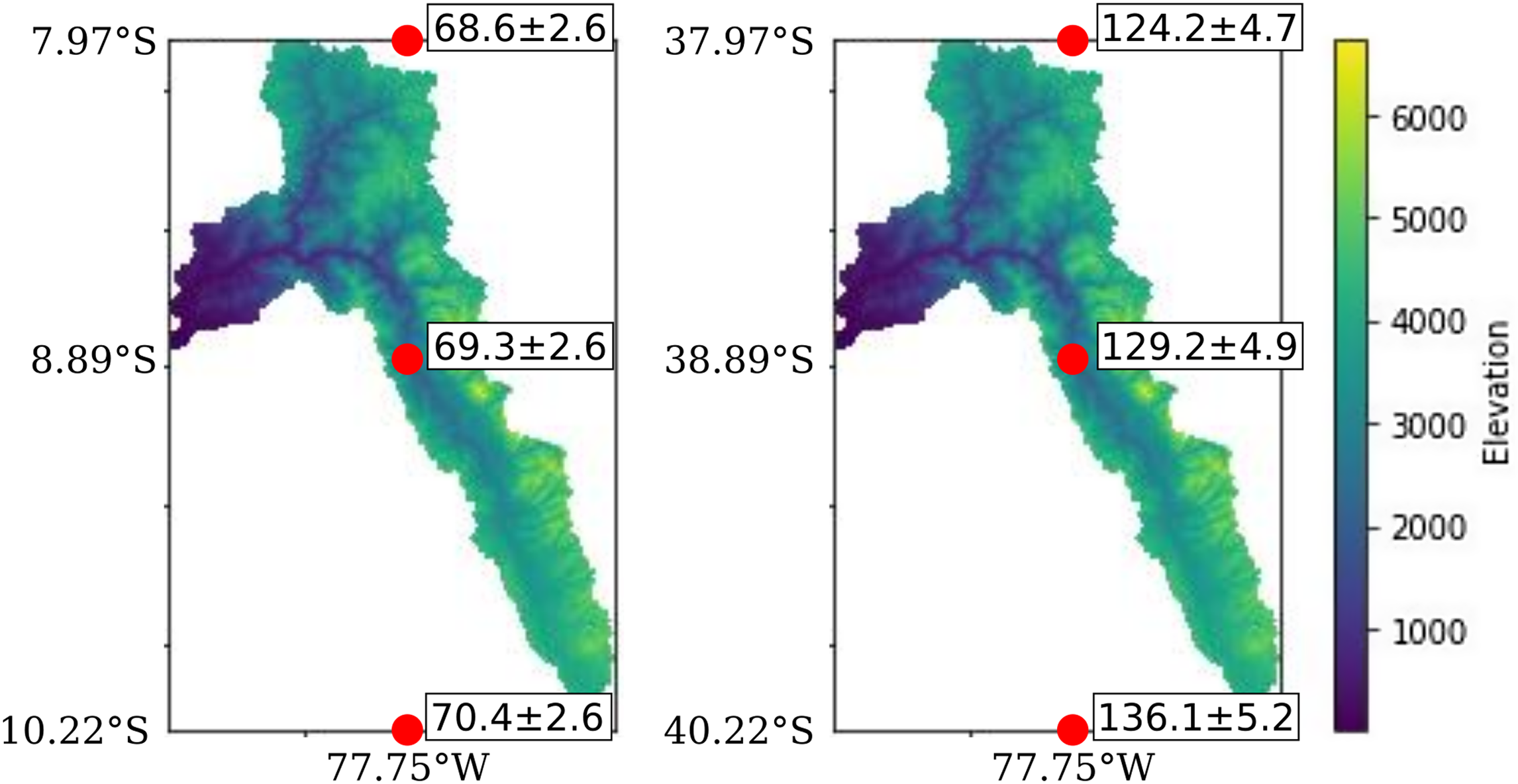
Figure 6 A simple test of latitudinal variation on predicted catchmentwide erosion rates using the PRCME-27 catchment of Reber et al. (Reference Reber, Delunel, Schlunegger, Litty, Madella, Akçar and Christl2017). (a) True location of the catchment, (b) catchment shifted 30° to the south to explore a medium-latitude setting. Red points and numbers show catchmentwide erosion rates (mm/kyr, LSDn scaling) calculated for three latitudes: The middle point is the catchment centroid, i.e., the default setting in the riversand calculator; the top and bottom points show the latitude of the northernmost and southermost tip of the catchment and corresponding erosion rates.
DISCUSSION
Previously published pixel-based approaches to catchmentwide erosion rate calculation (Mudd et al. Reference Mudd, Harel, Hurst, Grieve and Marrero2016; Charreau et al. Reference Charreau, Blard, Zumaque, Martin, Delobel and Szafran2019) achieve computational efficiency by using time-constant scaling methods, which do not take into account geomagnetic field fluctuations, based on the assertion that the differences between time-constant and time-dependent scaling are generally small. In two examples from the western Alps (∼45°N; Serra et al. Reference Serra, Valla, Delunel, Gribenski, Christl and Akçar2022) and the Peruvian Andes (2°S to 20°S; Reber et al. Reference Reber, Delunel, Schlunegger, Litty, Madella, Akçar and Christl2017), we show that erosion rates calculated with the St, Lm and LSDn scaling methods differ systematically by 5% to 20% (Figure 5a,b). In the latter example, the differences between time-constant and time-dependent scaling correlate with the erosion rate (Figure 5b) suggesting that the choice of a scaling method may result in a significant bias in the geological interpretion of the results.
Balco (Reference Balco2020) explored the effects of time-dependent (Lm, LSDn) vs. time-constant (St) scaling on calculated erosion rates by recalculating >3000 fluvial sediment datasets from the OCTOPUS database (Codilean et al. Reference Codilean, Munack, Cohen, Saktura, Gray and Mudd2018). The differences between time-dependent and time-constant methods vary systematically with erosion rate: for rates <100 mm/kyr the time-dependent results are up to 40% higher, for rates >100 mm/kyr time-dependent results are up to 30% lower than time-constant results (Figure 7). This means that ignoring geomagnetic field strength variations underestimates erosion rates in slowly eroding settings and overestimates rates in rapidly eroding settings. The trend is most pronounced at low latitudes (0–20°); at latitudes ≥40° time-dependent erosion rate estimates are ∼0–10% higher than time-constant results both in slowly and rapidly eroding settings. Although these calculations are based on catchment mean elevations instead of complete production rate models, the results are in excellent agreement with our findings: For the example from the Western Alps (300–1500 mm/kyr, ∼45°N), Balco (Reference Balco2020) predicts slightly higher results for LSDn than Lm scaling (<10%); our riversand calculations yield 5–10% higher values for LSDn compared to Lm (Figure 5a). For the example from the Peruvian Andes (10–200 mm/kyr, 6–20°S), Balco (Reference Balco2020) predicts that St scaling underestimates erosion by up to 20% for the slowly eroding catchments and overestimates erosion by up to 10% for the rapidly eroding catchments, a similar trend to what our riversand calculations show (Figure 5b).
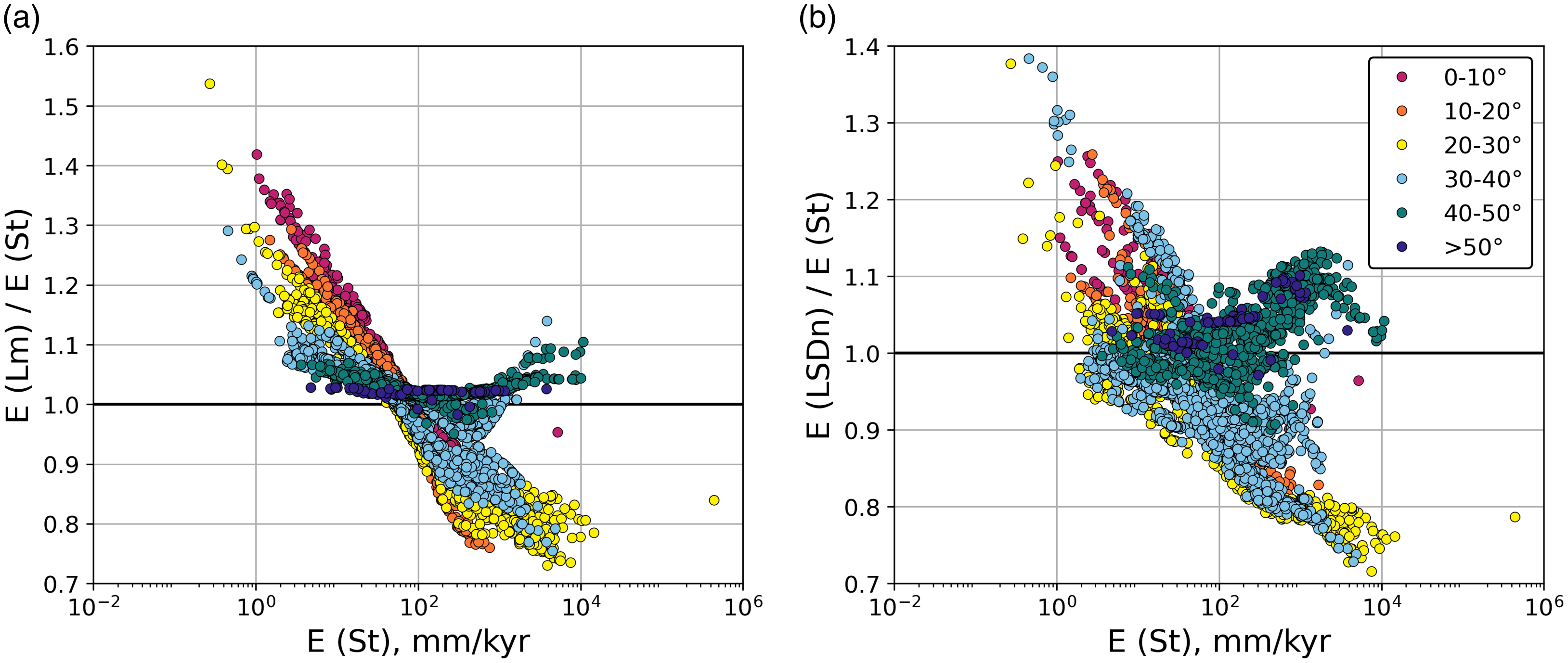
Figure 7 Comparison of time-dependent (a: Lm; b: LSDn) to time-constant (St) scaling for 4027 fluvial sediment datapoints from the OCTOPUS database (Codilean et al. Reference Codilean, Munack, Cohen, Saktura, Gray and Mudd2018) recalculated with the online erosion rate calculator. Calculations are based on catchment centroid coordinates and mean elevation. Data points are colored by latitude. The differences between time-dependent and time-constant methods vary systematically with erosion rate. Ignoring geomagnetic field strength variations underestimates erosion rates in slowly eroding settings and overestimates rates in rapidly eroding settings, the effect is most pronounced at low latitudes. See original analysis by Balco (Reference Balco2020).
The differences between time-constant and time-dependent erosion rate estimates and, in particular, their dependence on erosion rate can be explained in terms of the integration time of erosion T avg = z*/E (where the absorption length z* = 60 cm for an attenuation length of 160 g/cm² and a rock density of 2.7 g/cm³, e.g., Dunai Reference Dunai2010). An erosion rate of 100 mm/kyr corresponds to T avg = 6 kyr, i.e., rapidly eroding settings (∼1000 mm/kyr) integrate nuclide production over hundreds of years whereas slowly eroding settings (∼10 mm/kyr) integrate production over tens of thousands of years. Because the present magnetic field seems to be anomalously strong compared to the last few million years, samples from high-erosion settings have, on average, experienced higher magnetic field strengths and therefore lower production rates (Balco Reference Balco2020). Correcting for the effects of geomagnetic field strength variations (Lm, LSDn) therefore yields lower erosion-rate estimates in rapidly eroding settings and vice versa in slowly eroding settings.
Our hypsometry-based algorithm provides a fast and efficient means to calculate catchmentwide erosion rates. The comparison with two case studies shows that (1) our calculator reproduces the results of the pixel-based approaches within a few percent if a similar scaling method is chosen and (2) the results obtained with different scaling methods vary significantly (up to 20%). A simple approximation to catchmentwide erosion rates based on the catchment mean elevation can yield meaningful results, especially when dealing with large datasets (e.g., Balco Reference Balco2020), but the results may differ tens of percent from estimates that are based on a complete production rate model. Our algorithm currently does not take into account the latitudinal range of a catchment, and the calculator must be used with care when computing large (>2°) catchments at medium latitudes.
CONCLUSIONS
We present a new tool to calculate catchmentwide erosion rates from in situ 10Be (or 26Al) cosmogenic nuclide concentrations in alluvial sediments. The riversand calculator is distributed as a platform-independent, open-source python package. The processing of geospatial data (e.g., digital elevation model, topographic shielding data, catchment outline) is performed by the calculator. Production rate calculations are performed by the online exposure age and erosion rate calculator (Balco et al. Reference Balco, Stone, Lifton and Dunai2008), which is currently hosted on three servers (http://hess.ess.washington.edu, http://stoneage.ice-d.org, and http://stoneage.hzdr.de); by default, riversand sends its requests to http://stoneage.hzdr.de. This architecture guarantees that the results are based on the same production rates that are used by the online calculator to compute exposure ages and point-based erosion rates. Any future updates to the nuclide production scaling of the online calculator are immediately effective for the catchmentwide erosion rate calculation. Scaling methods used by the riversand calculator are those that are available from the online calculator (currently St, time-constant Lal/Stone; Lm, time-dependent Lal/Stone; LSDn, time-dependent and nuclide-specific Lifton/Sato/Dunai methods). In contrast to existing pixel-based approaches (Mudd et al. Reference Mudd, Harel, Hurst, Grieve and Marrero2016; Charreau et al. Reference Charreau, Blard, Zumaque, Martin, Delobel and Szafran2019), the computation time is identical for all scaling schemes, and the size and resolution of the catchment elevation model have little impact on the performance. Shielding by topography, vegetation or snow and ice can be set to a catchmentwide constant value or is derived from a raster dataset with the same projection and resolution as the elevation model. Heterogeneous quartz content in host rocks can be corrected for by a binary classification into “quartz-bearing” and “quartz-free” lithologies. The uncertainties on calculated erosion rates reflect only the analytical uncertainty on the measured nuclide concentration and correspond roughly to the “internal” uncertainties of the online calculator. A more realistic uncertainty estimate includes the uncertainties in production rates, uncertainties in shielding correction (topographic shielding and surface coverage) and the bias induced by non-uniform quartz distribution.
In two case studies, we show that erosion rates calculated with riversand agree with the results of pixel-based approaches within a few percent if based on the same scaling method. Scaling methods that do not account for geomagnetic field variations may overpredict or underpredict erosion rates by >20%, especially for rapidly (≥1000 mm/kyr) or slowly (≤10 mm/kyr) eroding settings at low latitudes (Balco Reference Balco2020). Therefore, the time-dependent, nuclide-specific LSDn scaling method (Lifton et al. Reference Lifton, Sato and Dunai2014) should be the preferred scaling method for catchmentwide erosion rate calculations. Uncertainties returned by the riversand calculator reflect the analytical uncertainty in cosmogenic nuclide measurements (“internal uncertainty”). The package including documentation is available from https://pypi.org/project/riversand/.
SUPPLEMENTARY MATERIAL
To view supplementary material for this article, please visit https://doi.org/10.1017/RDC.2023.74
ACKNOWLEDGMENTS
We acknowledge funding by the German Science Foundation (DFG grant STU 525/2-2 awarded to KS). This work greatly benefitted from instructive discussions at the Radiocarbon-24 conference in Zürich and with the AMS group at Helmholtz-Zentrum Dresden-Rossendorf. We thank Christopher T. Halsted for his careful review of the manuscript and Timothy Jull and Kimberley T. Elliott for editorial handling.


 Open access