


INTRODUCTION
The spatiotemporal variability of marine radiocarbon (14C) records is superimposed by a systematic isotopic depletion with respect to the atmosphere. This effect is frequently expressed as marine reservoir age (MRA) and has to be taken into account when 14C calibration considers marine archives (Alves et al. Reference Alves, Macario, Ascough and Bronk Ramsey2018). Prebomb MRAs have ranged from ~400 yr in subtropical oceans to more than 1000 yr in polar seas (Key et al. Reference Key, Kozyr, Sabine, Lee, Wanninkhof, Bullister, Feely, Millero, Mordy and Peng2004). Prior to the continuous tree-ring record, MRAs are poorly constrained and have to be inferred from ad-hoc assumptions or through modeling.
IntCal20 aims to reconstruct the atmospheric 14C concentration at mid-latitudes in the Northern Hemisphere. From 0 to ~13.9 cal kBP, IntCal20 is constructed from dendrochronologically dated tree rings providing direct atmospheric observation. However, further back in time, the lack of available trees means that a variety of alternative archives are required including macro-fossils, speleothems, corals and planktic foraminifera. Each of these archives have their own specific characteristics. In particular, the use of data from marine environments (such as corals and foraminifera) is complicated by the MRA meaning such observations are offset, probably floating in space and time, from the atmospheric 14C we wish to reconstruct. To reliably reconstruct atmospheric 14C, we therefore need to be able to resolve such records into their constituent atmospheric and MRA components.
To provide such a resolution for IntCal20, we have taken the following approach. Firstly, we construct a preliminary estimate for atmospheric 14C based solely upon the Hulu cave record (Southon et al. Reference Southon, Noronha, Cheng, Edwards and Wang2012; Cheng et al. Reference Cheng, Edwards, Southon, Matsumoto, Feinberg, Sinha, Zhou, Li, Li and Xu2018). This Hulu-Cave-based atmospheric 14C reconstruction is then fed into an ocean general circulation model (Butzin et al. Reference Butzin, Köhler and Lohmann2017) to provide temporal MRA estimates at all of our marine sites contributing to IntCal. These MRA estimates are then fed back into the construction of the main IntCal20 atmospheric curve allowing us to compile the MRA-adjusted marine records alongside the other archives, see Heaton et al. (Reference Heaton, Blaauw, Blackwell, Bronk Ramsey, Reimer and Scott2020 in this issue) for further details. Such an approach can be seen somewhat analogously to the first step in an iterative backfitting procedure (or a single update of the MRA within a wider Markov Chain Monte Carlo method). While ideally one may wish to iterate this procedure several times to improve MRA estimation, we believe a single run will provide a reliable first-order approximation. Here, we give an overview of the applied simulation scenarios to create these MRA estimates given the Hulu-Cave-based curve and briefly discuss the results.
METHOD
We employ the Hamburg Large Scale Geostrophic (LSG) ocean general circulation model (Maier-Reimer et al. Reference Maier-Reimer, Mikolajewicz and Hasselmann1993) with a horizontal resolution of 3.5° and a vertical resolution of 22 unevenly spaced levels. The LSG model has been constantly improved by including a bottom boundary layer scheme (Lohmann Reference Lohmann1998), a sophisticated numerical advection scheme (Schäfer-Neth and Paul Reference Schäfer-Neth, Paul, Schäfer, Ritzrau, Schlüter and Thiede2001; Prange et al. Reference Prange, Lohmann and Paul2003) and has demonstrated its skills in 14C simulations (Butzin et al. Reference Butzin, Prange and Lohmann2005, Reference Butzin, Prange and Lohmann2012, Reference Butzin, Köhler and Lohmann2017). In the current setup, the model can simulate the entire radiocarbon timescale (~60 kyr) within a few days of CPU time on state-of-the-art computer systems. The model is forced with monthly fields of recent and glacial wind stress, surface air temperature, and freshwater flux derived in previous climate simulations (Lohmann and Lorenz Reference Lohmann and Lorenz2000; Prange et al. Reference Prange, Lohmann, Romanova and Butzin2004). In the same way as in our precursor study (Butzin et al. Reference Butzin, Köhler and Lohmann2017), we consider three climate forcing scenarios to assess the impact of past ocean-climate variability on marine 14C records. To summarize, scenario PD employs present-day climate background conditions approximating the Holocene and interstadials. Glacial scenario GS aims at representing the Last Glacial Maximum (LGM), featuring a shallower Atlantic meridional overturning circulation (AMOC) weakened by about 30% compared to PD. A second glacial climate scenario (CS) mimics cold stadials with further AMOC weakening by about 60%. A thorough discussion of these scenarios can be found in Butzin et al. (Reference Butzin, Prange and Lohmann2005).
Radiocarbon is simulated on-line as F 14R oce-atm (the 14C enrichment of the ocean relative to the contemporaneous atmosphere, Soulet et al. Reference Soulet, Skinner, Beaupré and Galy2016) following Toggweiler et al. (Reference Toggweiler, Dixon and Bryan1989). That is, we do not consider 14C and 12C separately but directly simulate their fractionation-corrected ratio. This approach neglects biological effects which are one order of magnitude smaller than the effects of ocean circulation and radioactive decay on F 14R oce-atm (Fiadeiro Reference Fiadeiro1982). Oceanic uptake of 14C is calculated according to Sweeney et al. (Reference Sweeney, Gloor, Jacobson, Key, McKinley, Sarmiento and Wanninkhof2007), using atmospheric CO2 concentrations as compiled in the spline of Köhler et al. (Reference Köhler, Nehrbass-Ahles, Schmitt, Stocker and Fischer2017) and prescribed time-invariant concentrations of dissolved inorganic carbon in surface water as simulated by Hesse et al. (Reference Hesse, Butzin, Bickert and Lohmann2011). As described in the introduction, atmospheric 14C forcing was based solely upon the Hulu Cave speleothem record with a Dead Carbon Fraction (DCF) of about (450 ± 70) 14C yr (Southon et al. Reference Southon, Noronha, Cheng, Edwards and Wang2012; Cheng et al. Reference Cheng, Edwards, Southon, Matsumoto, Feinberg, Sinha, Zhou, Li, Li and Xu2018). To create this Hulu-Cave-based atmospheric curve, the same Bayesian spline errors-in-variables statistical methodology was used as in construction of the final IntCal20 curve (Heaton et al. Reference Heaton, Blaauw, Blackwell, Bronk Ramsey, Reimer and Scott2020 in this issue). Within each individual speleothem, the DCF was considered constant but taking potentially different levels for each speleothem in the cave. Priors for the DCF of each speleothem were taken from the relevant papers of Southon et al. (Reference Southon, Noronha, Cheng, Edwards and Wang2012) and Cheng et al. (Reference Cheng, Edwards, Southon, Matsumoto, Feinberg, Sinha, Zhou, Li, Li and Xu2018). The spline-based Markov Chain Monte Carlo (MCMC) was run for 250,000 iterations (with the first half being discarded as burn-in) to obtain a posterior mean estimate for the Hulu-based 14C atmospheric reconstruction along with upper and lower 95% credible (2-sigma) pointwise intervals (see Figure 1).
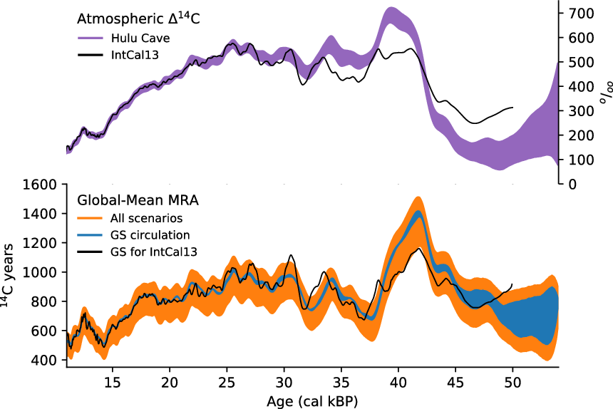
Figure 1 (Top) Atmospheric Δ14C from the Hulu Cave record (Southon et al. Reference Southon, Noronha, Cheng, Edwards and Wang2012; Cheng et al. Reference Cheng, Edwards, Southon, Matsumoto, Feinberg, Sinha, Zhou, Li, Li and Xu2018) used as transient forcing in our simulations. Plotted band spans the uncertainty range (mean values ±2 σ). (Bottom) Simulated global mean marine reservoir ages (MRA) in the upper 50 m, plotted are global averages excluding regions poleward of 50° latitude. Upper and lower bounds of all results are plotted in orange. Scenario GS is plotted in blue. The black lines show previous model results for scenario GS (Butzin et al. Reference Butzin, Köhler and Lohmann2017) forced with atmospheric Δ14C according to IntCal13 (Reimer et al. Reference Reimer, Bard, Bayliss, Beck, Blackwell, Bronk Ramsey, Buck, Cheng, Edwards, Friedrich, Grootes, Guilderson, Haflidason, Hajdas, Hatté, Heaton, Hoffman, Hogg, Hughen, Kaiser, Kromer, Manning, Niu, Reimer, Richards, Scott, Southon, Staff, Turney and van der Plicht2013). (Please see electronic version for color figures.)
We combine all three ocean climates (PD, GS, and CS) and all three 14C forcing scenarios (posterior mean, upper and lower 95% credible intervals) to create nine numerical experiments. Each experiment is spun up over 20,000 yr with fixed atmospheric values of 14C and CO2 at 54 cal kBP (Δ14Catm = 73–504‰ and pCO2 = 219 μatm), before the model is run transiently forward in time until 10.7 cal kBP forced by time-variable 14C and pCO2 values. Marine reservoir ages are calculated afterwards in 14C-yr as MRA = –8033 × ln (F 14R oce-atm), based on simulation results for the upper 50 m of the ocean corresponding to the typical habitat depth of corals and foraminifera analyzed in IntCal20. The impact of different ocean surface depth ranges on MRA has been analyzed in Butzin et al. (Reference Butzin, Köhler and Lohmann2017) and is not investigated any further here.
RESULTS AND DISCUSSION
Figure 1 shows the simulated history of global-mean MRAs. The envelope spans all MRA simulations and may be interpreted as total uncertainty range. A closer look at the MRA uncertainty of any specific ocean climate scenario, e.g. scenario GS, indicates that the contribution of the atmospheric 14C forcing uncertainty is small between 10.7 and ~44 cal kBP. That is, the uncertainty of simulated MRAs is largely due to the difference in the three climate scenarios, with the upper or lower bound corresponding to scenario CS or PD, respectively.
In the following discussion we focus on scenario GS, as (most) MRA estimates in IntCal20 are based on this scenario, which also corresponds to the ensemble median of simulated MRAs when forced with the mean atmospheric 14C record. Disregarding high-latitude regions where sea ice inhibits oceanic 14CO2 uptake, we find global mean MRA variations between 500 and 1400 14C yr. The lowest reservoir ages are simulated during the last deglaciation with two minima around 11 and 14 cal kBP caused by the combination of small atmospheric 14C values and rising concentrations of atmospheric CO2, the latter allowing a higher oceanic 14CO2 uptake. At the LGM (19–23 cal kBP) the global mean MRA was about 800 14C yr. Prior to the LGM our simulations show variations in global mean MRA of several hundreds of years with positive anomalies associated with the Mono Lake (~34 cal kBP, Lund et al. Reference Lund, Benson, Negrini, Liddicoat and Mensing2017) and Laschamps (~42 cal kBP, Lascu et al. Reference Lascu, Feinberg, Dorale, Cheng and Edwards2016) geomagnetic excursions. In our precursor study (considering scenario GS and atmospheric 14C according to IntCal13, black line in Figure 1) the amplitude of these variations was slightly larger between 27 cal kBP and 34 cal kBP, but more than 200 14C yr smaller around the Laschamps excursion. This is due to the revised atmospheric 14C forcing during this period. Note that the global mean MRA peak at 42 cal kBP precedes the atmospheric 14C maximum by about 3000 cal yr. Instead, the global mean MRA peak coincides with an inflection point of the atmospheric 14C forcing curve after which the slowly adjusting ocean is able to catch up with the 14C excursion in the atmosphere.
Since the climate scenarios applied here are identical to those used in our previous work, we also find—as expected—similar results: the youngest surface waters are always found in the subtropical oceans and the oldest surface waters in the polar seas, where ice cover can boost MRAs to more than 3000 14C yr. During the LGM the general spatial pattern of the MRA is in line with the few data-based MRA reconstructions (Skinner et al. Reference Skinner, Primeau, Freeman, Fuente, Goodwin, Gottschalk, Huang, McCave, Noble and Scrivner2017) available for this time slice (Figure 2).
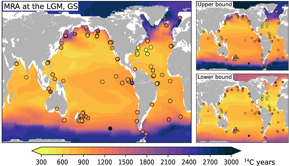
Figure 2 Geographic distribution of simulated marine reservoir ages (MRAs) in the upper 50 m at the Last Glacial Maximum (time average over 19–23 cal kBP). Left: Results for scenario GS forced with the mean atmospheric Δ14C record; right: upper and lower bounds of all simulation results involving scenarios CS (top) and PD (bottom). Filled circles are foraminifera-based MRAs compiled by Skinner et al. (Reference Skinner, Primeau, Freeman, Fuente, Goodwin, Gottschalk, Huang, McCave, Noble and Scrivner2017).
Here, the lowest MRAs are simulated for the subtropical Northeast Pacific where 14C paleorecords are particularly scarce. However, in no scenario we arrive at such low MRAs close to preindustrial values as contained in the reconstruction for the subtropical Northwest Atlantic (Skinner et al. Reference Skinner, Primeau, Freeman, Fuente, Goodwin, Gottschalk, Huang, McCave, Noble and Scrivner2017). To assess potential model biases not only for a single date but for the entire simulation period, we compare reconstructed marine Δ14C records contributing to IntCal20 with marine Δ14C simulated at nearby grid cells, keeping in mind that none of these sites is representative for open-ocean conditions for which the LSG model has been designed. This is shown as scatterplot in Figure 3, in which unbiased model results and reconstructions should align along a straight line with slope = 1 and intercept = 0. Our simulations frequently underestimate marine Δ14C prior to ~30 cal kBP where the uncertainties in the reconstructions are large. Simulated Δ14C is also low in the Cariaco Basin prior to ~19 cal kBP.
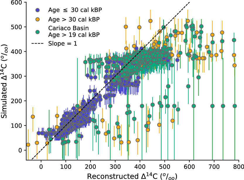
Figure 3 Comparison of simulated and reconstructed marine Δ14C for locations which contain records contributing to IntCal20 (Bard et al. Reference Bard, Hamelin, Fairbanks and Zindler1990, Reference Bard, Arnold, Hamelin, Tisnerat-Laborde and Cabioch1998, Reference Bard, Rostek and Ménot-Combes2004a, Reference Bard, Ménot-Combes and Rostek2004b, Reference Bard, Ménot, Rostek, Licari, Böning, Edwards, Cheng, Wang and Heaton2013; Burr et al. Reference Burr, Beck, Taylor, Recy, Edwards, Cabioch, Correge, Donahue and O’Malley1998, Reference Burr, Galang, Taylor, Gallup, Edwards, Cutler and Quirk2004; Hughen et al. Reference Hughen, Southon, Lehman and Overpeck2000, Reference Hughen, Southon, Bertrand, Frantz and Zermeño2004, Reference Hughen, Southon, Lehman, Bertrand and Turnbull2006; Cutler et al. Reference Cutler, Gray, Burr, Edwards, Taylor, Cabioch, Beck, Cheng and Moore2004; Fairbanks et al. Reference Fairbanks, Mortlock, Chiu, Cao, Kaplan, Guilderson, Fairbanks, Bloom, Grootes and Nadeau2005; Durand et al. Reference Durand, Deschamps, Bard, Hamelin, Camoin, Thomas, Henderson, Yokoyama and Matsuzaki2013; Heaton et al. Reference Heaton, Bard and Hughen2013). Simulation results are for ocean climate scenario GS forced with the mean atmospheric Δ14C record where error bars indicate the combined uncertainty of atmospheric Δ14C and scenarios CS and PD. Four data points are not shown (two data points with reconstructed Δ14C < –150‰ and simulated Δ14C ~20‰, plus two data points with reconstructed Δ14C > 1500‰ and simulated Δ14C ~200‰).
The underestimate of simulated Δ14C suggests that the MRAs derived for these data points may be too high or that much of the coral data older than 30 ka BP has undergone diagenesis. The Cariaco Basin Δ14C data could be reconciled with our simulations by assuming unrealistically large variations in the dead carbon fraction of the Hulu Cave 14C record. Instead, IntCal20 has used another approach (Bayesian adaptive learning, see Heaton et al. Reference Heaton, Blaauw, Blackwell, Bronk Ramsey, Reimer and Scott2020 in this issue) to estimate past MRAs in this specific marine environment. The LSG model resolution of ~380 km in the region of the Cariaco Basin is too coarse to capture its small depression (160 km long, 60 km wide) on the continental shelf off Venezuela, which was decoupled from the open Caribbean during the last glacial sea level lowstand (Peterson et al. Reference Peterson, Overpeck, Kipp and Imbrie1991). First MRA simulations utilizing a global ocean general circulation model with enhanced resolution down to ~20 km in marginal seas (FESOM2 developed by Danilov et al. Reference Danilov, Sidorenko, Wang and Jung2017) show promising improvements for the Cariaco region but long-term simulations, which would be necessary for a potential application of FESOM2 within this calibration effort here, are not yet available.
ACKNOWLEDGMENTS
This work was supported by the German Federal Ministry of Education and Research (BMBF) as Research for Sustainable Development (FONA; http://www.fona.de) through the PalMod project (grant number: 01LP1505B). Model results are available at PANGAEA, https://doi.pangaea.de/10.1594/PANGAEA.902301


 Open access