


1. Introduction
Temporal logic (TL) is arguably the primary language for the formal specification and reasoning about system correctness and safety. It has been successfully applied to the analysis of a wide range of systems, including cyber-physical systems (Bartocci et al., Reference Bartocci, Deshmukh, Donzé, Fainekos, Maler, Nickovic and Sankaranarayanan2018), programs (Manna and Pnueli, Reference Manna and Pnueli2012), and stochastic models (Kwiatkowska et al., Reference Kwiatkowska, Norman and Parker2007). In cyber-physical systems, TLs are especially useful for expressing and verifying critical properties of these systems, to ensure systems meet performance and safety criteria. For example, (probabilistic) TLs can express safety and reachability properties (e.g., ‘will the system eventually reach the goal state(s) while avoiding unsafe states?”) and fault-tolerance properties (e.g., ‘will the system return to some desired service level after a fault?”).
However, a limitation of existing TLs is that TL specifications must be evaluated on a fixed configuration of the system, for example a fixed choice of control policy, communication protocol, or system dynamics. That is, they cannot express queries like ‘what is the probability that the system throughput will stay above a certain threshold if we switch to a high-performance controller?”, or ‘what would have been the probability that the signal would have stayed below a given threshold if we had used a different policy in the past?” This kind of reasoning about different system conditions falls under the realm of causal inference (Pearl, Reference Pearl2009), by which the first query is called an intervention and the second a counterfactual. Even though both causal inference and TL-based verification are well-established on their own, their combination hasn’t been sufficiently explored in past literature (see Section 7 for a more complete account of the related work). With this paper, we contribute to bridging these two fields.
We introduce PCFTL (Probabilistic CounterFactual Temporal Logic), the first probabilistic temporal logic that explicitly includes causal operators to express interventional properties (‘what will happen if…”), counterfactual properties (‘what would have happened if…”), and so-called causal effects, defined as the difference of interventional or counterfactual probabilities between two different configurations. In particular, in this paper we focus on the analysis of Markov Decision Processes (MDPs), which are capable of modeling sequential decision-making processes under uncertainty, a key aspect in many cyber-physical systems applications. MDPs provide a useful framework for a variety of applications, such as reinforcement learning, planning, and probabilistic verification. For MDPs, arguably the most relevant kind of causal reasoning concerns evaluating how a change in the MDP policy affects some outcome. The outcome of interest for us is the satisfaction probability of a temporal-logic formula.
Interventions are ‘forward-looking” (Oberst and Sontag, Reference Oberst and Sontag2019), as they allow us to evaluate the probability of a TL property ϕ after applying a particular change X ← X′ to the system. Counterfactuals are instead ‘retrospective” (Oberst and Sontag, Reference Oberst and Sontag2019), telling us what might have happened under a different condition: having observed an MDP path τ, they allow us to evaluate ϕ on the what-if version of τ, that is the path that we would have observed if we had applied X ← X′ at some point in the past, provided that the random factors that yielded τ remain fixed. Causal effects (Guo et al., Reference Guo, Cheng, Li, Hahn and Liu2020) allow us to establish the impact of a given change at the level of the individual path or overall, and they quantify the increase in the probability of ϕ induced by a manipulation X ← X′. Causal and counterfactual reasoning has gained a lot of attention in recent years due to its power in observational data studies: with counterfactuals, one can answer what-if questions relative to an observed path, that is without having to intervene on the real system (which might jeopardize safety) but using observational data only. Our PCFTL logic enables this kind of reasoning in the context of formal verification.
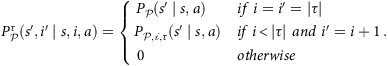
Our approach to incorporating causal inference in temporal logic involves only a minimal extension of traditional probabilistic logics. PCFTL is an extension of PCTL⋆ (Baier et al., 1997; Baier, 1998) where the probabilistic operator P ⋈ p (ϕ), which checks whether the probability of ϕ satisfies threshold ⋈ p (where ⋈ ∈ {≤, <, >, ≥ }), is replaced with a counterfactual operator I @t .P ⋈ p (ϕ), which concerns the probability of ϕ if we had applied intervention I at t time steps in the past. Albeit minimal, such an extension provides great expressive power: if t > 0, then the operator corresponds to a counterfactual query; if t = 0, it represents an interventional probability; if both t = 0 and I is empty, then we retrieve the traditional P ⋈ p (ϕ) operator.
Motivating example: To better grasp interventions and counterfactuals, consider an example of a robot in a 2D space, modeled by the equation S
t + 1 = S
t
+ A
t
+ U
t
, where S
t
∈ ℝ2 and A
t
∈ ℝ2 are the state and action at time t, and U
t
∈ ℝ2 is an unobserved random exogenous input (e.g., white Gaussian noise). The robot must satisfy a bounded safety property ϕ = ¬ℱ[1,4](S
t
≥ [1, 2]), which specifies that the robot must avoid entering the unsafe region S
t
≥ [1, 2] on all paths (up to length 3) that it takes. Suppose we observe a path τ under some policy π, given by $\tau = [0, 0]{ [0, 1]\atop{\longrightarrow}} [0.1, 0.5] {[1,1]\atop{\longrightarrow}} [0.8, 1.75] {[0, 0]\atop{\longrightarrow}}[1.3, 2.1]$
, where
$\tau = [0, 0]{ [0, 1]\atop{\longrightarrow}} [0.1, 0.5] {[1,1]\atop{\longrightarrow}} [0.8, 1.75] {[0, 0]\atop{\longrightarrow}}[1.3, 2.1]$
, where $s{ a\atop{\longrightarrow}}s'$
denotes a step from state s to s′ through action a. This path, and hence policy π, is unsafe because it violates the safety property in its final state. A question then arises: given τ, if we had intervened in the past by changing the policy from π to some π′, could have we prevented this violation? Define the intervention
$s{ a\atop{\longrightarrow}}s'$
denotes a step from state s to s′ through action a. This path, and hence policy π, is unsafe because it violates the safety property in its final state. A question then arises: given τ, if we had intervened in the past by changing the policy from π to some π′, could have we prevented this violation? Define the intervention $I = \pi \leftarrow \pi^\prime$
. Then, the counterfactual PCFTL query I
@3.P
⋈ p
(ϕ) allows us to evaluate the probability of the safety property ϕ in a what-if version of τ where we apply I (i.e., policy π′ instead of π) at 3 steps back from the last state of τ, that is from the beginning of the path in this case.Footnote
1
In particular, the counterfactual path is obtained by applying I but by keeping the same values of the random exogenous factors U
t
that led to τ. These factors cannot be directly observed, but, given the above Equation, they can be readily determined as U
t
= S
t + 1 − S
t
− A
t
, leading to U
1 = [0.1,−0.5], U
2 = [−0.3,0.25], and U
3 = [0.5,0.35]. Then, suppose the alternative policy π′ chooses actions A′1 = [0,0.5] and A′3 = [−0.4,−0.2] (but keeps A′2 = A
2), then this induces the counterfactual path
$I = \pi \leftarrow \pi^\prime$
. Then, the counterfactual PCFTL query I
@3.P
⋈ p
(ϕ) allows us to evaluate the probability of the safety property ϕ in a what-if version of τ where we apply I (i.e., policy π′ instead of π) at 3 steps back from the last state of τ, that is from the beginning of the path in this case.Footnote
1
In particular, the counterfactual path is obtained by applying I but by keeping the same values of the random exogenous factors U
t
that led to τ. These factors cannot be directly observed, but, given the above Equation, they can be readily determined as U
t
= S
t + 1 − S
t
− A
t
, leading to U
1 = [0.1,−0.5], U
2 = [−0.3,0.25], and U
3 = [0.5,0.35]. Then, suppose the alternative policy π′ chooses actions A′1 = [0,0.5] and A′3 = [−0.4,−0.2] (but keeps A′2 = A
2), then this induces the counterfactual path $\tau '= [0,0]{ [0, 0.5]\atop{\longrightarrow}} [0.1, 0] {[1, 1]\atop{\longrightarrow}} [0.8, 1.25] {[-0.4, -0.2]\atop{\longrightarrow}} [0.9, 1.4]$
. Notably, now τ′ satisfies the safety property.
$\tau '= [0,0]{ [0, 0.5]\atop{\longrightarrow}} [0.1, 0] {[1, 1]\atop{\longrightarrow}} [0.8, 1.25] {[-0.4, -0.2]\atop{\longrightarrow}} [0.9, 1.4]$
. Notably, now τ′ satisfies the safety property.
Despite the simplicity of this example, counterfactual reasoning becomes challenging when dealing with discrete-state probabilistic models like MDPs. Indeed, the state of an MDP evolves according to a categorical distribution, for which the identification and inference of the exogenous factors are non-trivial.
Contributions: In this paper, we introduce the syntax and semantics of PCFTL and present a statistical model-checking approach for verifying PCFTL properties in MDP environments. Our approach, summarized in Figure 1, relies on translating the MDP into a so-called structural causal model (SCM), a fundamental model in causal inference that enables computation of counterfactual distributions. We use a particular form of SCMs (Oberst and Sontag, Reference Oberst and Sontag2019) suitable for encoding categorical counterfactuals (arising with discrete-state MDPs). After performing counterfactual inference, the SCM model is then translated back into an MDP amenable for PCFTL model checking. Unlike existing logics, PCFTL formulas are interpreted with respect to an observed MDP path τ, rather than a single MDP state, as we must keep track of the past to perform counterfactual reasoning.
Using efficient statistical model checking procedures, we evaluate PCFTL on a reinforcement learning benchmark (Chevalier-Boisvert et al., Reference Chevalier-Boisvert, Willems and Pal2018) involving multiple 2D grid-world environments, goal-oriented tasks, and interventional and counterfactual properties under various policies learned through neural-network-based reinforcement learning methods. These results demonstrate the usefulness of PCFTL in AI safety, but our approach could enhance the verification of probabilistic models in a variety of domains, from distributed systems to security and biology.
The paper covers background about SCMs, MDPs, and SCM-based encoding of MDPs in Section 2, construction of counterfactual MDPs in Section 3, definition of PCFTL syntax, semantics, and decision procedures in Section 4, experimental results in Section 6, related work in Section 7, and conclusions in Section 8.
2. Background
2.1. Causal inference with structural causal models
Structural Causal Models (SCMs) (Pearl, Reference Pearl2009; Glymour et al., Reference Glymour, Pearl and Jewell2016) are equation-based models to specify and reason about causal relationships involving some variables of interest.
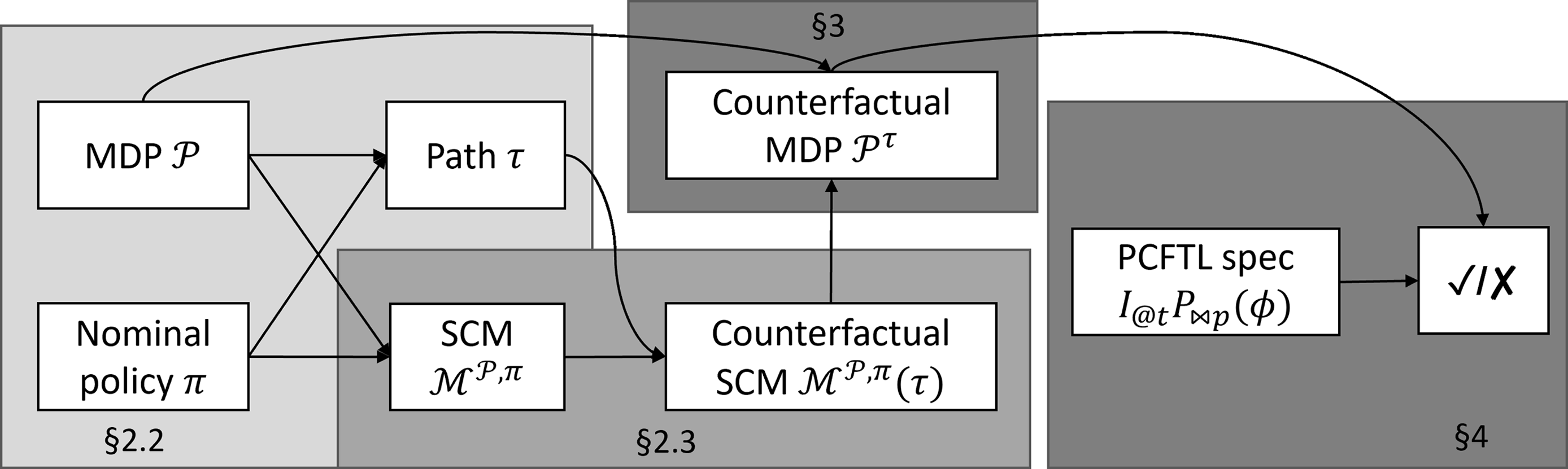
Figure 1. Overview of our approach to PCFTL verification, with section pointers.
Definition 1 (Structural Causal Model (SCM))
An SCM is a tuple ${{\cal {M}}} =({\bf {U}},{\bf {V}}, {\cal {F}}, P({\bf {U}}))$
where
${{\cal {M}}} =({\bf {U}},{\bf {V}}, {\cal {F}}, P({\bf {U}}))$
where
- ${\bf {U}}$
is a set of (mutually independent) exogenous variables.
${\bf {U}}$
is a set of (mutually independent) exogenous variables.
-
${\bf {V}}$
is a set of endogenous variables, where the value of each
$V \in {\bf {V}}$
is determined by a function
$V = f_V({\bf {PA}}_V, U_V)$
. Here,
${\bf {PA}}_V \subseteq {\bf {V}}$
are the set of direct causes of V, and
$U_V\in {\bf {U}}$
.
-
ℱ is the set of functions
$\{\,f_V\}_{V \in {\bf {V}}}$
. -
$P({\bf {U}})=\bigotimes _{U \in {\bf {U}}} P(U)$
is the joint distribution of the (mutually independent) exogenous variables.


Assignments in ℱ must be acyclic, to ensure that no variable can be a direct or indirect cause of itself. Because of this, the causal relationships in an SCM can be represented by a directed acyclic graph (DAG), called a causal diagram.
In an SCM, the values of the exogenous variables ${\bf {U}}$
are determined by factors outside the model, which is modelled by some distribution
${\bf {U}}$
are determined by factors outside the model, which is modelled by some distribution $P({\bf {U}})$
. Exogenous variables are unobserved variables which act as the source of randomness in the system. Indeed, for a fixed realization
$P({\bf {U}})$
. Exogenous variables are unobserved variables which act as the source of randomness in the system. Indeed, for a fixed realization $\mathbf {u}$
of
$\mathbf {u}$
of ${\bf {U}}$
, that is a concrete unfolding of the system’s randomness, the values of
${\bf {U}}$
, that is a concrete unfolding of the system’s randomness, the values of ${\bf {V}}$
become deterministic, as they are uniquely determined by
${\bf {V}}$
become deterministic, as they are uniquely determined by $\mathbf {u}$
and the causal processes ℱ. A concrete value
$\mathbf {u}$
and the causal processes ℱ. A concrete value $\mathbf {u}$
of
$\mathbf {u}$
of ${\bf {U}}$
is also called context (or unit). We denote by
${\bf {U}}$
is also called context (or unit). We denote by $P_{{\cal {M}}}({\bf {V}})$
the so-called observational distribution of
$P_{{\cal {M}}}({\bf {V}})$
the so-called observational distribution of ${\bf {V}}$
, that is, the data-generating distribution entailed by the SCM ℱ and
${\bf {V}}$
, that is, the data-generating distribution entailed by the SCM ℱ and $P({\bf {U}})$
.
$P({\bf {U}})$
.
Interventions. With SCMs, one can establish the causal effect of some input variable X on some output variable Y by evaluating Y after ‘forcing” some specific values x on X, an operation called intervention. Applying X←x means replacing the RHS of $X = f_X({\bf {PA}}_X, U_X)$
with x. Interventions allow to establish the true causal effect of X on Y by comparing the so-called post-interventional distribution P
ℳ[X←x](Y) at different values x, where ℳ[X←x] is the SCM obtained from ℳ by applying X ← x.Footnote
2
By ‘disconnecting” X from any of its possible causes, interventions prevent any source of spurious association between X and Y (Glymour et al., Reference Glymour, Pearl and Jewell2016) (i.e., caused by variables other than X and that are not descendants of X).Footnote
3
In the following we will use the notation I (and ℳ[I]) to denote a set of interventions I = {V
i
← v
i
}
i
.
$X = f_X({\bf {PA}}_X, U_X)$
with x. Interventions allow to establish the true causal effect of X on Y by comparing the so-called post-interventional distribution P
ℳ[X←x](Y) at different values x, where ℳ[X←x] is the SCM obtained from ℳ by applying X ← x.Footnote
2
By ‘disconnecting” X from any of its possible causes, interventions prevent any source of spurious association between X and Y (Glymour et al., Reference Glymour, Pearl and Jewell2016) (i.e., caused by variables other than X and that are not descendants of X).Footnote
3
In the following we will use the notation I (and ℳ[I]) to denote a set of interventions I = {V
i
← v
i
}
i
.
Counterfactuals. Upon observing a particular realization ${\bf {v}}$
of the SCM variables
${\bf {v}}$
of the SCM variables ${\bf {V}}$
, counterfactuals answer the following question: what would have been the value of some variable Y for observation
${\bf {V}}$
, counterfactuals answer the following question: what would have been the value of some variable Y for observation ${\bf {v}}$
if we had applied intervention I on our model ℳ? This corresponds to evaluating
${\bf {v}}$
if we had applied intervention I on our model ℳ? This corresponds to evaluating ${\bf {V}}$
in a hypothetical world characterized by the same context (i.e., same realization of random factors) that generated the observation
${\bf {V}}$
in a hypothetical world characterized by the same context (i.e., same realization of random factors) that generated the observation ${\bf {v}}$
but under a different causal process.
${\bf {v}}$
but under a different causal process.
Computing counterfactuals involves three steps (Glymour et al., Reference Glymour, Pearl and Jewell2016):
-
1. abduction: estimate the context given the observation, that is derive
${P({\bf {U}} \mid {\bf {V}}=\bf {v}})$
; -
2. action: modify the SCM by applying the intervention of interest, for example ℳ[I]; and
-
3. prediction: evaluate
${\bf {V}}$
under the manipulated model ℳ[I] and the inferred context.


We denote by ${{\cal {M}}({\bf {v}}})[I]$
the counterfactual model obtained by replacing
${{\cal {M}}({\bf {v}}})[I]$
the counterfactual model obtained by replacing $P({\bf {U}})$
with
$P({\bf {U}})$
with ${P({\bf {U}} \mid {\bf {V}}=\bf {v}})$
in the SCM ℳ and then applying intervention I. Note that here
${P({\bf {U}} \mid {\bf {V}}=\bf {v}})$
in the SCM ℳ and then applying intervention I. Note that here ${\bf {v}}$
is a realization of
${\bf {v}}$
is a realization of ${\bf {V}}$
under ℳ and not under ℳ[I].
${\bf {V}}$
under ℳ and not under ℳ[I].
As explained above, each observation ${{\bf {V}}=\bf {v}}$
can be seen as a deterministic function of a particular value
${{\bf {V}}=\bf {v}}$
can be seen as a deterministic function of a particular value $\mathbf {u}$
of
$\mathbf {u}$
of ${\bf {U}}$
. Therefore, the counterfactual model is deterministic too, assuming that such
${\bf {U}}$
. Therefore, the counterfactual model is deterministic too, assuming that such $\mathbf {u}$
can be identified from
$\mathbf {u}$
can be identified from ${{\bf {V}}=\bf {v}}$
. However, inferring
${{\bf {V}}=\bf {v}}$
. However, inferring $\mathbf {u}$
precisely is often not possible (as discussed later), resulting in a (non-Dirac) posterior distribution of contexts
$\mathbf {u}$
precisely is often not possible (as discussed later), resulting in a (non-Dirac) posterior distribution of contexts ${P({\bf {U}} \mid {\bf {V}}=\bf {v}})$
and thus, a stochastic counterfactual value.
${P({\bf {U}} \mid {\bf {V}}=\bf {v}})$
and thus, a stochastic counterfactual value.
2.1.1. Causal effects
Estimating a causal effect amounts to comparing some variable Y (outcome, output) under different values of some other variable X (treatment, input). Interventions and counterfactuals enable this task by ruling out spurious association between X and Y, as discussed above. There are three main estimators of causal effects:
Individual Treatment Effect (ITE). For a context $\mathbf {u}$
, the ITE of
$\mathbf {u}$
, the ITE of $Y\in {\bf {V}}$
between interventions I
1 and I
0 is defined as
$Y\in {\bf {V}}$
between interventions I
1 and I
0 is defined as $Y_{I_1}(\mathbf {u})-Y_{I_0}(\mathbf {u})$
, where
$Y_{I_1}(\mathbf {u})-Y_{I_0}(\mathbf {u})$
, where $Y_{I_i}(\mathbf {u})$
is the counterfactual value of Y induced by
$Y_{I_i}(\mathbf {u})$
is the counterfactual value of Y induced by $\mathbf {u}$
under the post-intervention model ℳ[I
i
]. As explained above, we don’t have direct access to the exogenous values
$\mathbf {u}$
under the post-intervention model ℳ[I
i
]. As explained above, we don’t have direct access to the exogenous values $\mathbf {u}$
but only to realizations
$\mathbf {u}$
but only to realizations ${\bf {v}} \sim P_{{\cal {M}}}({\bf {V}})$
. Thus, below we define the ITE as a function of
${\bf {v}} \sim P_{{\cal {M}}}({\bf {V}})$
. Thus, below we define the ITE as a function of ${\bf {v}}$
(rather than
${\bf {v}}$
(rather than $\mathbf {u}$
) by plugging in the average counterfactual value of Y w.r.t. the posterior
$\mathbf {u}$
) by plugging in the average counterfactual value of Y w.r.t. the posterior ${P({\bf {U}} \mid {\bf {V}}=\bf {v}})$
:
${P({\bf {U}} \mid {\bf {V}}=\bf {v}})$
:
 $${\textit {ITE}(Y,I_1,I_0,{\bf {v}}}) = {\mathbb {E}}_{{\cal {M}}({\bf {v}})[I_1]}[Y] - {\mathbb {E}}_{{\cal {M}}({\bf {v}})[I_0]}[Y]. $$
Average Treatment Effect (ATE). ATE is used to estimate causal effects at the population level and is defined as the expected value (w.r.t. $P({\bf {U}})$
) of the individual treatment effect, or equivalently, as the difference of post-interventional expectations:
$P({\bf {U}})$
) of the individual treatment effect, or equivalently, as the difference of post-interventional expectations:
 $$ \textit {ATE}(Y,I_1,I_0)= {\mathbb {E}}_{{\cal {M}}[I_1]}[Y] - {\mathbb {E}}_{{\cal {M}}[I_0]}[Y]. $$
Conditional Average Treatment Effect (CATE). The CATE is the conditional version of ATE. This estimator is useful when the treatment effect may vary across the population depending on the value of some variables V:
 $$ \textit {CATE}(Y,I_1,I_0,v)= {\mathbb {E}}_{{\cal {M}}[I_1]}[Y\mid V=v] - {\mathbb {E}}_{{\cal {M}}[I_0]}[Y\mid V=v]. $$
2.2. Markov Decision Processes (MDPs)
MDPs are a class of stochastic models to describe sequential decision making processes, where at each step t, an agent in state s i performs some action a i determined by a policy π ending up in state s i + 1 ∼ P(⋅ ∣ s i , a i ). The agent receives some reward ℛ(s i , a i ) for performing a i at s i . Here, we focus on MDPs with finite state and action spaces. Without loss of generality, we restrict the policy class to deterministic policies (Puterman, Reference Puterman2014). Moreover, each MDP state satisfies a (possibly empty) set of atomic propositions, with AP being the set of atomic propositions.
Definition 2 (Markov Decision Process (MDP))
An MDP is a tuple 𝒫 = (𝒮, 𝒜, P 𝒫, P I , ℛ, L) where 𝒮 is the state space, 𝒜 is the set of actions, P 𝒫 : (𝒮 × 𝒜 × 𝒮)→[0,1] is the transition probability function, P I : 𝒮 → [0,1] is the initial state distribution, ℛ : (𝒮 × 𝒜) → ℝ is the reward function, and L : 𝒮 → 2 AP is a labelling function, which assigns to each state s ∈ 𝒮 the set of atomic propositions that are valid in s. A (deterministic) policy π for 𝒫 is a function π : 𝒮 → 𝒜.
An agent acting under policy π in an MDP environment will induce an MDP path τ, as follows:
Definition 3 (MDP path)
A path τ = (s
1, a
1), (s
2, a
2), … of an MDP 𝒫 = (𝒮, 𝒜, P
𝒫, P
I
, ℛ, L) induced by a policy π is a sequence of state-action pairs where s
i
∈ 𝒮 and a
i
= π(s
i
) for all i ≥ 1. The probability of a path τ is given by $P_{\cal {P}}(\tau ) = P_I(s_1)\cdot \prod _{i\geq 1} P_{\cal {P}}(s_{i+1}\mid s_i, a_i)$
. For a finite path τ = (s
1, a
1), …, (s
$P_{\cal {P}}(\tau ) = P_I(s_1)\cdot \prod _{i\geq 1} P_{\cal {P}}(s_{i+1}\mid s_i, a_i)$
. For a finite path τ = (s
1, a
1), …, (s $ {\text k} $
, a
$ {\text k} $
, a $ {\text k} $
), we denote by Paths
𝒫, π
(τ) the set of all (infinite) paths with prefix τ induced by MDP 𝒫 and policy π, which has probability P
𝒫(Paths
𝒫, π
(τ)) = P
𝒫(τ).
$ {\text k} $
), we denote by Paths
𝒫, π
(τ) the set of all (infinite) paths with prefix τ induced by MDP 𝒫 and policy π, which has probability P
𝒫(Paths
𝒫, π
(τ)) = P
𝒫(τ).
We denote by |τ| the length of the path, by τ[i] the i-th element of τ (for 0 < i ≤ |τ|), by τ[i :] the suffix of τ starting at position i (inclusive), and by τ[i : i + j] the subsequence spanning positions i to i + j (inclusive). Even though τ[i] denotes the pair (s i , a i ) of the path, we will often use it, when the context is clear, to denote only the state s i . We slightly abuse notation and write Paths 𝒫, π (s) to denote the set of paths induced by π and starting with s.
Usually, an MDP is stationary, meaning that its transition probability function and/or reward function remain fixed over time. However, there exists a variant, called a non-stationary MDP (Lecarpentier and Rachelson, Reference Lecarpentier, Rachelson, Wallach, Larochelle, Beygelzimer, d’Alché-Buc, Fox and Garnett2019), where the transition probability function and/or reward function may change over time. A non-stationary MDP can be converted to a stationary MDP by augmenting its state space with a variable that keeps track of the time.
An MDP under a fixed policy can be described as a deterministic-time Markov Chain (DTMC), as follows.
Definition 4 (Induced DTMC)
An MDP 𝒫 = (𝒮, 𝒜, P 𝒫 P I ,R, L) and a policy π : 𝒮 → 𝒜 induce a discrete-time Markov Chain (DTMC) 𝒟𝒫, π = (𝒮, P 𝒟𝒫, π , P I , R 𝒫, π , L) where for s, s′ ∈ 𝒮, P 𝒟𝒫, π (s′∣s) = P 𝒫(s′ ∣ s, π(s)), and for s ∈ 𝒮, R 𝒫, π (s) = R(s, π(s)). Paths of 𝒟𝒫, π are sequences of states, and their probabilities are defined similarly to Def. 3 .
2.3. SCM-based encoding of MDPs
We now present the SCM-based encoding of MDPs introduced in (Oberst and Sontag, Reference Oberst and Sontag2019). For a given path length T, the SCM ℳ𝒫, π, T induced by an MDP 𝒫 and a policy π characterizes the unrolling of paths of 𝒫 of length T, that is it has endogenous variables S t and A t describing the MDP’s state and action at each time step t, where t = 1, …, T. These are defined by the structural equations:
 $$ S_{t+1} = f(S_{t},A_{t}, U_{t}); \quad A_t = \pi (S_t); \quad S_1 = f_0(U_0), $$
where the probabilistic state transition at t, P 𝒫(S t + 1 ∣ S t , A t ), is encoded as a deterministic function f of S t , A t , and the (random) exogenous variables U t , while the random choice of the initial state, P I (S 1), as a deterministic function f 0 of U 0.
We stress that the SCM encoding does not require any assumptions about the structure of the MDP: such encoding results in an acyclic graph, while the original MDP need not be. Figure 2 shows the causal diagram resulting from this SCM encoding.
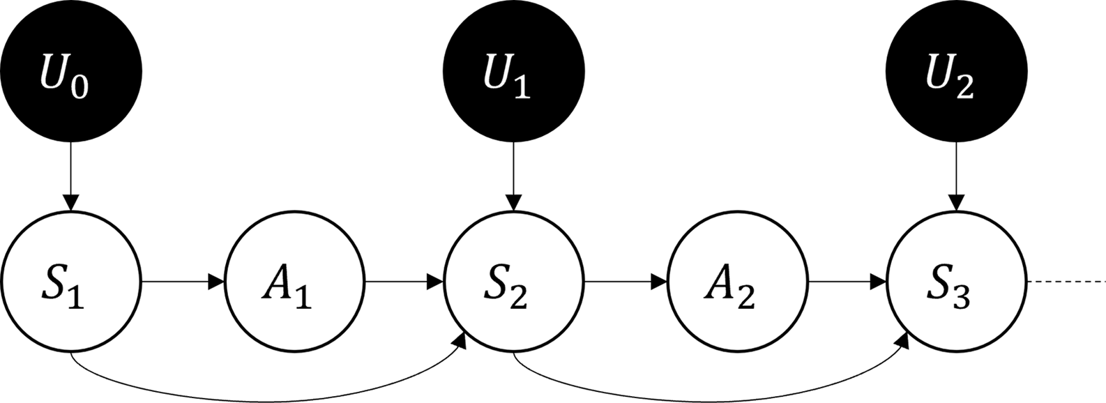
Figure 2. Causal diagram for the SCM encoding of an MDP. Black circles represents exogenous variables, while white circles represent endogenous ones.
Note that both P 𝒫(S t + 1 ∣ S t , A t ) and P I (S 1) are categorical distributions and encoding them in the above SCM form (i.e., as functions of a random variable) is not obvious. Oberst and Sontag (Reference Oberst and Sontag2019) proposed a solution termed Gumbel-Max SCM, as given by:
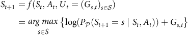 $$\begin{gathered}{S_{t + 1}} = f({S_t},{A_t},{U_t} = {({G_{s,t}})_{s \in S}}) \\ \,\,\,\,\,\,\,\,\,\,\,\,\,\,\,\,\,\,\,\,\,\,\,\,\,\,\,\,\,\,\,\,\,\,\,\,\,\,\,\,\,\,\,\,\,\,\,\,\,\,\,\,\,\,\,\,\,\,\,\,\,\,\,\,\,\,\,\,\,\,\,= \begin{array}{*{20}{c}}{arg{\mkern 1mu} max} \\ \small{s \in S} \\ \end{array} \left\{ {\log \left( {{P_P}({S_{t + 1}} = s\mid {S_t},{A_t})} \right) + {G_{s,t}}} \right\} \\ \end{gathered}$$
where, for s ∈ 𝒮 and t ∈ 1 = …, T, G
s, t
∼ Gumbel. This is based on the Gumbel-Max trick, by which one can sample from a categorical distribution with $ {\cal k} $
categories (corresponding to the |S| MDP states in our case) by first drawing realizations g
1, …, g
$ {\cal k} $
categories (corresponding to the |S| MDP states in our case) by first drawing realizations g
1, …, g $ {\cal k} $
of a standard Gumbel distribution and then by setting the outcome to arg max
j
{log(P(Y = j))+g
j
}. By using the Gumbel-Max trick, the assignment S
t + 1 = f(S
t
, A
t
, (G
s, t
)
s ∈ 𝒮) in (5) will be equivalent to sampling S
t + 1 ∼ P
𝒫(S ∣ S
t
, A
t
):
$ {\cal k} $
of a standard Gumbel distribution and then by setting the outcome to arg max
j
{log(P(Y = j))+g
j
}. By using the Gumbel-Max trick, the assignment S
t + 1 = f(S
t
, A
t
, (G
s, t
)
s ∈ 𝒮) in (5) will be equivalent to sampling S
t + 1 ∼ P
𝒫(S ∣ S
t
, A
t
):
Proposition 1 (Gumbel-Max SCM correctness)
Given an MDP 𝒫, policy π, and time bound T, then for any path τ of 𝒫 induced by π of length T, we have P ℳ𝒫, π, T (τ) = P 𝒫(τ), where ℳ𝒫, π, T is the Gumbel-Max SCM for 𝒫, π, and T.
Importantly, the Gumbel-Max SCM encoding enjoys a desirable property called counterfactual stability:
Definition 5 (Counterfactual stability (Oberst and Sontag, Reference Oberst and Sontag2019))
An SCM ℳ satisfies counterfactual stability relative to a categorical variable Y of ℳ if whenever we observe Y = i under some intervention I, then the counterfactual value of Y under I′ ≠ I remains Y = i unless I′ increases the relative likelihood of an alternative outcome j ≠ i, that is unless P ℳ[I′](Y=j)/P ℳ[I](Y=j) > P ℳ[I′](Y=i)/P ℳ[I](Y=i).
Intuitively, the above definition tells us that, in a counterfactual scenario, we would observe the same outcome Y = i unless the intervention increases the relative likelihood of an alternative outcome Y = j, that is, unless $ {{p_j'}\over {p_j}} \gt {{p_i'}\over {p_i}}$
holds for some j.
$ {{p_j'}\over {p_j}} \gt {{p_i'}\over {p_i}}$
holds for some j.
Gumbel-Max SCMs are the most prominent encoding that can express categorical variables as functions of independent random variables and that satisfy counterfactual stability.Footnote 4 However, there also exists methods that generalise to other causal mechanisms with the counterfactual stability property (see Section 7).
Counterfactual inference. Given we observed an MDP path τ = (s 1,a 1), …, (s |τ|,a |τ|), counterfactual inference in this setting entails deriving P((G s, t ) s ∈ 𝒮 t = 1, …, |τ| − 1 ∣τ). Essentially, this means finding values for the Gumbel exogenous variables compatible with τ. By the Markov property, the above can be factorized as follows:
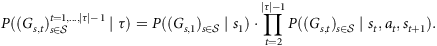 $$P((G_{s,t})_{s\in \cal {S}}^{t=1,\ldots, |\tau |-1}\mid \tau )= P((G_{s,1})_{s\in \cal {S}} \mid s_1) \cdot \prod _{t=2}^{|\tau |-1} P((G_{s,t})_{s\in \cal {S}}\mid s_t,a_t,s_{t+1}).$$
However, the mechanism of (5) is non-invertible, i.e., given s t and a t , there might be multiple values of (G s, t ) s ∈ 𝒮 leading to the same s t + 1. This implies that MDP counterfactuals can’t be uniquely identified, a problem that affects categorical counterfactuals in general and not just Gumbel-Max SCMs (Oberst and Sontag, Reference Oberst and Sontag2019).
As suggested by Oberst and Sontag (Reference Oberst and Sontag2019), we can perform (approximate) posterior inference of P((G s, t ) s ∈ 𝒮∣s t ,a t ,s t + 1) through rejection sampling. This involves sampling from the prior P((G s, t ) s ∈ 𝒮), and rejecting all the realizations (g s, t ) s ∈ 𝒮 for which f(s t ,a t ,(g s, t ) s ∈ 𝒮) ≠ s t + 1.
Interventions in MDPs. In principle, we can consider any kind of intervention I over the SCM encoding of an MDP. Arguably, the most relevant case is when I affects the MDP policy π. For instance, in some applications, we might want to replace π with a more conservative or aggressive policy. Hence, in the following, we assume interventions of the form I = {(π←π′)} for some policy π′ (i.e., we change the RHS of the equation for A t in the SCM (4)).
Example 1 (MDP counterfactuals)
Consider an MDP model of a light switch. The MDP has two states, ${\cal S} = \{ \mathsf On, Off \}$
, and we can take two actions,
${\cal S} = \{ \mathsf On, Off \}$
, and we can take two actions, ${\cal A} = \{ \mathsf Switch, Nop \}$
. If we take action
${\cal A} = \{ \mathsf Switch, Nop \}$
. If we take action $\mathsf Switch$
, the state of the MDP changes (from
$\mathsf Switch$
, the state of the MDP changes (from $\mathsf On$
, to
$\mathsf On$
, to $\mathsf Off$
, or vice versa) with probability 0.9, and it remains the same with probability 0.1. If we take action
$\mathsf Off$
, or vice versa) with probability 0.9, and it remains the same with probability 0.1. If we take action $\mathsf Nop$
, with probability 0.9 the MDP’s state does not change, and with probability 0.1 the state changes. We fix the following policy: π(
$\mathsf Nop$
, with probability 0.9 the MDP’s state does not change, and with probability 0.1 the state changes. We fix the following policy: π( $\mathsf On$
) =
$\mathsf On$
) = $\mathsf NOP$
and π(
$\mathsf NOP$
and π( $\mathsf Off$
) =
$\mathsf Off$
) = $\mathsf Switch$
.
$\mathsf Switch$
.
Assume we observe the path $\tau = {\mathsf Off} {{\mathsf {\ Switch\ }}\atop{\longrightarrow}}\mathsf {On\ } {{\mathsf {\ NOP\ }}\atop{\longrightarrow}} \mathsf {Off}$
, where the first step has probability 0.9 and the second step 0.1. First, we want to show that the Gumbel-max SCM formulation
(5)
yields the same probability values, modulo sampling variability. In Figure 3a and Figure 3b we show the values of log (P
𝒫(
$\tau = {\mathsf Off} {{\mathsf {\ Switch\ }}\atop{\longrightarrow}}\mathsf {On\ } {{\mathsf {\ NOP\ }}\atop{\longrightarrow}} \mathsf {Off}$
, where the first step has probability 0.9 and the second step 0.1. First, we want to show that the Gumbel-max SCM formulation
(5)
yields the same probability values, modulo sampling variability. In Figure 3a and Figure 3b we show the values of log (P
𝒫( $\mathsf Off\,$
∣S
t
,A
t
)) + G
$\mathsf Off\,$
∣S
t
,A
t
)) + G $\mathsf Off$
, t (x-axis) and log (P
𝒫(
$\mathsf Off$
, t (x-axis) and log (P
𝒫( $\mathsf On\,$
∣S
t
,A
t
)) + G
$\mathsf On\,$
∣S
t
,A
t
)) + G $\mathsf On$
, t (y-axis) obtained by sampling 1000 realizations of the Gumbel variables
$\mathsf On$
, t (y-axis) obtained by sampling 1000 realizations of the Gumbel variables $\bf {G}$
. We see indeed that, at t = 2, 89.7% of these points lie above the identity line, that is they yield
$\bf {G}$
. We see indeed that, at t = 2, 89.7% of these points lie above the identity line, that is they yield $\mathsf On$
as the next state. At t = 3, we find that 10.9% of the points yield
$\mathsf On$
as the next state. At t = 3, we find that 10.9% of the points yield $\mathsf Off$
as the next state.
$\mathsf Off$
as the next state.
In Figure 3c and Figure 3d, we show the computation of counterfactuals. Assume an intervention that changes the policy into one that constantly performs action $\mathsf Switch$
. Now, we want to see what is the probability of path
$\mathsf Switch$
. Now, we want to see what is the probability of path $\tau ' = {\mathsf Off} {{\mathsf {\ Switch\ }}\atop{\longrightarrow}}\mathsf {On\ } {{\mathsf {\ Switch\ }}\atop{\longrightarrow}} \mathsf {Off}$
given that we observed τ. That is, we compute the probability of τ′ in the counterfactual SCM model where the (prior) Gumbel variables are replaced by
$\tau ' = {\mathsf Off} {{\mathsf {\ Switch\ }}\atop{\longrightarrow}}\mathsf {On\ } {{\mathsf {\ Switch\ }}\atop{\longrightarrow}} \mathsf {Off}$
given that we observed τ. That is, we compute the probability of τ′ in the counterfactual SCM model where the (prior) Gumbel variables are replaced by ${\bf {G}'=\mathbf {G}}\mid \tau$
, that is those inferred from τ.
${\bf {G}'=\mathbf {G}}\mid \tau$
, that is those inferred from τ.
First note that τ and τ′ perform the same first step. Hence, this step has probability 1 under ${\bf {G}}'$
because
${\bf {G}}'$
because ${\bf {G}}'$
is defined such that it assigns probability 1 to the observed path (see also Proposition 3 for a similar statement). In the second step, the observed path τ transitioned into
${\bf {G}}'$
is defined such that it assigns probability 1 to the observed path (see also Proposition 3 for a similar statement). In the second step, the observed path τ transitioned into $\mathsf Off$
after performing Nop, despite a probability of 0.9 of jumping into
$\mathsf Off$
after performing Nop, despite a probability of 0.9 of jumping into $\mathsf On$
. This means that
$\mathsf On$
. This means that ${\bf {G}}'$
strongly favours
${\bf {G}}'$
strongly favours $\mathsf Off$
(over
$\mathsf Off$
(over $\mathsf On$
) to happen in the second step. Hence, we expect that the probability of
$\mathsf On$
) to happen in the second step. Hence, we expect that the probability of ${\mathsf On} {{\mathsf {\ Switch\ }}\atop{\longrightarrow}}\mathsf {Off}$
in the counterfactual world will be higher than the nominal probability P
𝒫(
${\mathsf On} {{\mathsf {\ Switch\ }}\atop{\longrightarrow}}\mathsf {Off}$
in the counterfactual world will be higher than the nominal probability P
𝒫( $\mathsf Off$
∣
$\mathsf Off$
∣ $\mathsf On$
,
$\mathsf On$
, $\mathsf Switch$
). In particular, by counterfactual stability (Def. 5), such probability should be 1 because the intervention doesn’t make state
$\mathsf Switch$
). In particular, by counterfactual stability (Def. 5), such probability should be 1 because the intervention doesn’t make state $\mathsf On$
more likely to happen (rather the opposite: the relative likelihood of
$\mathsf On$
more likely to happen (rather the opposite: the relative likelihood of $\mathsf On$
is indeed 0.1/0.9, while it is 0.9/0.1 for
$\mathsf On$
is indeed 0.1/0.9, while it is 0.9/0.1 for $\mathsf Off$
). This can be proven also by showing that, by rejection sampling, we have that:
$\mathsf Off$
). This can be proven also by showing that, by rejection sampling, we have that:
 $$P_{{\bf {G}}'}\left (\log \left (P_{\cal {P}}(\mathsf {Off} \mid \mathsf {On}, \mathsf {Nop})\right ) + G'_{\mathsf {Off},t} \gt \log \left (P_{\cal {P}}(\mathsf {On} \mid \mathsf {On}, \mathsf {Nop})\right ) + G'_{\mathsf {On},t}\right ) = 1.$$
Since 0.9 = P
𝒫( $\mathsf Off$
∣
$\mathsf Off$
∣ $\mathsf On, Switch$
) > P
𝒫(
$\mathsf On, Switch$
) > P
𝒫( $\mathsf Off$
∣
$\mathsf Off$
∣ $\mathsf On, NOP$
) = 0.1 and 0.1 = P
𝒫(
$\mathsf On, NOP$
) = 0.1 and 0.1 = P
𝒫( $\mathsf On$
∣
$\mathsf On$
∣ $\mathsf On, Switch$
) < P
𝒫(
$\mathsf On, Switch$
) < P
𝒫( $\mathsf On$
∣
$\mathsf On$
∣ $\mathsf On, NOP$
) = 0.9, it follows that
$\mathsf On, NOP$
) = 0.9, it follows that
 $$P_{{\bf {G}}'}\left (\log \left (P_{\cal {P}}(\mathsf {Off} \mid \mathsf {On}, \mathsf {Switch})\right ) + G'_{\mathsf {Off},t} \gt \log \left (P_{\cal {P}}(\mathsf {On} \mid \mathsf {On}, \mathsf {Switch})\right ) + G'_{\mathsf {On},t}\right ) = 1,$$
i.e., performing action $\mathsf Switch$
at state
$\mathsf Switch$
at state $\mathsf On$
has probability 1 of leading into state
$\mathsf On$
has probability 1 of leading into state $\mathsf Off$
in the counterfactual world. In particular, since P
𝒫(
$\mathsf Off$
in the counterfactual world. In particular, since P
𝒫( $\mathsf Off$
∣
$\mathsf Off$
∣ $\mathsf On, Switch$
) > P
𝒫(
$\mathsf On, Switch$
) > P
𝒫( $\mathsf Off$
∣
$\mathsf Off$
∣ $\mathsf On, NOP$
), the points in Figure 3d (corresponding to the counterfactual step) are shifted to the right compared to Figure 3b (observed step).
$\mathsf On, NOP$
), the points in Figure 3d (corresponding to the counterfactual step) are shifted to the right compared to Figure 3b (observed step).
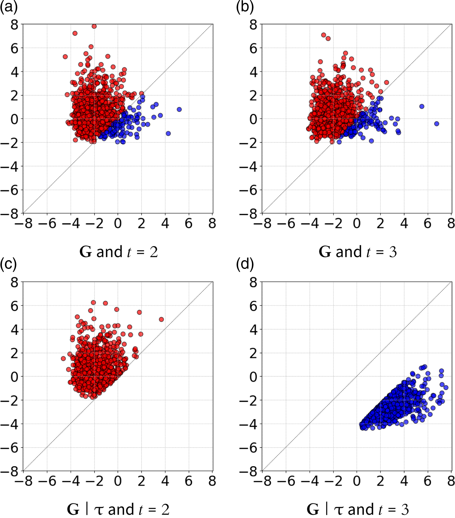
Figure 3. Light switch MDP (example 1). X-axis: log (P
𝒫( $\rm\mathsf Off $
∣S
t
, A
t
)) + G
$\rm\mathsf Off $
∣S
t
, A
t
)) + G $\rm\mathsf Off$
, t; Y-axis: log (P
𝒫(
$\rm\mathsf Off$
, t; Y-axis: log (P
𝒫( $\rm\mathsf On$
∣S
t
, A
t
)) + G
$\rm\mathsf On$
∣S
t
, A
t
)) + G $\rm\mathsf On$
, t. Plots (a) and (b) are relative to the prior Gumbel G and the observed path τ (using 1000 realizations for G). Plots (c) and (d) are relative to the posterior Gumbel G τ and the counterfactual path τ′. Points leading to state
$\rm\mathsf On$
, t. Plots (a) and (b) are relative to the prior Gumbel G and the observed path τ (using 1000 realizations for G). Plots (c) and (d) are relative to the posterior Gumbel G τ and the counterfactual path τ′. Points leading to state $\rm\mathsf On$
are in red, while those for
$\rm\mathsf On$
are in red, while those for $\rm\mathsf Off$
are in blue.
$\rm\mathsf Off$
are in blue.
3. Construction of counterfactual MDP
Consider a Gumbel-max SCM ℳ𝒫 for an MDP 𝒫 under policy π, and a (finite) path τ of ℳ𝒫. Let ${\bf {G}}'=(G'_{s,i})_{s\in \cal {S}}^{i=1,\ldots, |\tau |-1}$
be the set of posterior Gumbel variables, where, for i = 1, …, |τ| − 1, G′
s, i
∼ P
ℳ𝒫
(G
s, i
∣τ) and G
s, i
∼ Gumbel. That is, G′
s, i
is the value of the exogenous variable (associated to position i and state s) inferred from τ. Then, for i = 1, …, |τ| − 1, we have the following transition probability function, which directly follows from the SCM (5):
${\bf {G}}'=(G'_{s,i})_{s\in \cal {S}}^{i=1,\ldots, |\tau |-1}$
be the set of posterior Gumbel variables, where, for i = 1, …, |τ| − 1, G′
s, i
∼ P
ℳ𝒫
(G
s, i
∣τ) and G
s, i
∼ Gumbel. That is, G′
s, i
is the value of the exogenous variable (associated to position i and state s) inferred from τ. Then, for i = 1, …, |τ| − 1, we have the following transition probability function, which directly follows from the SCM (5):
See also (Tsirtsis, De, and Rodriguez, Reference Tsirtsis, De and Rodriguez2021) for a similar definition. Then, we can express this non-stationary MDP as a stationary one by augmenting its state space as follows.
Definition 6 (Counterfactual MDP)
Given an MDP 𝒫, policy π, and a finite path τ of 𝒫 under π, the corresponding (stationary) counterfactual MDP 𝒫τ = (𝒮τ, 𝒜, P 𝒫τ, P I τ, ℛ′, L′). Here, 𝒮τ = 𝒮 × {1, …, |τ|} is an augmented state space where each state s′ ∈ 𝒮τ corresponds to a tuple s′ = (s, i), where each state s ∈ 𝒮 from the nominal MDP 𝒫 has been augmented with a timestep i, ℛ′ : (𝒮τ × 𝒜) → ℝ is a reward function such that ℛ′((s, i), a) = ℛ(s, a), L′ : 𝒮τ → 2 AP is a labelling function such that L′((s, i)) = L(s), P I τ(τ[1],1) = 1, and for any (s, i), (s′, i′) ∈ 𝒮τ and a ∈ 𝒜,
In other words, in 𝒫τ we introduce an extra variable to track the position i of the observed path τ. Then, for i < |τ|, 𝒫τ behaves according to the transition probabilities of the counterfactual model, as per Eq. 6. For i = |τ|, 𝒫τ is equivalent to the original MDP model 𝒫, because we do not have an observation on which we can condition our Gumbel exogenous variables. Also, P I τ is defined such that 𝒫τ admits only one initial state, that is, the first state of τ. The following proposition shows that the counterfactual MDP reduces to the original MDP in the special case when |τ| = 1.
Proposition 2. If |τ| = 1, then the counterfactual MDP 𝒫τ of an MDP 𝒫 is equivalent to 𝒫(τ[1]).
Proof. It is easy to see that, by applying Def. 6, we recover the definition of the original MDP 𝒫 (with the provision that 𝒮τ = 𝒮 × {1}) initialised at τ[1], the only state of τ. Indeed, if τ contains only one state, then we do not have any observed transitions to perform posterior inference of the Gumbel exogenous variables.□
Another useful property is that if we do not perform any interventions, that is we maintain the original policy π, then the counterfactual MDP induces the observed path τ with probability 1, as expected.
Proposition 3. Given 𝒫, π, and τ as per Definition 6 , then the resulting counterfactual MDP 𝒫τ is such that P 𝒫τ (τ) = 1.
Proof. It is enough to show that, for any 1 ≤ i < |τ|, it holds that
This is true because the posterior Gumbel variables G′ s″, i are inferred in order to be consistent with the observed path. This holds also for (approximate) inference via rejection sampling: since we discard all the Gumbel realizations incompatible with the observation, we have that
which proves the above equality.□
In the following, for simplicity, we will use policies π defined over 𝒮 (the state space of the original MDP 𝒫) also for the augmented state space 𝒮τ of the counterfactual MDP, by assuming π(s, i) = π(s) for any i.
4. PCFTL: a probabilistic temporal logic with interventions, Counterfactuals, and Causal Effects
In this section, we formally define PCFTL (Probabilistic CounterFactual Temporal Logic). A PCFTL formula is interpreted over an MDP 𝒫, a policy π, and an observed path τ resulting from 𝒫 and π.
PCFTL extends PCTL⋆ (Baier et al., 1997; Baier, 1998) with a counterfactual operator I
@t
.P
⋈ p
(ϕ), a counterfactual reward operator I
@t
.R
⋈ r
≤ $ {\cal k} $
, and two causal effect operators,
$ {\cal k} $
, and two causal effect operators, $ \Delta_{@t}^{{I_{1}}, {I_{0}}}$
.P
⋈ p
(ϕ) and
$ \Delta_{@t}^{{I_{1}}, {I_{0}}}$
.P
⋈ p
(ϕ) and $ \Delta_{@t}^{{I_{1}}, {I_{0}}}$
.R
⋈ r
≤
$ \Delta_{@t}^{{I_{1}}, {I_{0}}}$
.R
⋈ r
≤ $ {\cal k} $
. The latter two formulas are defined as the difference of counterfactual probabilities (resp., cumulative rewards) between interventions I
1 and I
0, in line with the definition of treatment effects in Section 2.1.
$ {\cal k} $
. The latter two formulas are defined as the difference of counterfactual probabilities (resp., cumulative rewards) between interventions I
1 and I
0, in line with the definition of treatment effects in Section 2.1.
PCFTL syntax. The syntax of PCFTL is as follows:
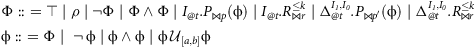 $$\small{ \eqalign{ & \Phi ::\ = \top \mid \rho \mid \neg \Phi \mid \Phi \wedge \Phi \it \mid {I_{@t}}.{P_{\Join p}}({\rm \phi}) \mid {I_{@t}}.R_{\Join r}^{ \le k}\mid \Delta _{@t}^{{I_1},{I_0}}.{P_{\Join p'}}({\rm \phi} )\mid \Delta _{@t}^{{I_1},{I_0}}.R_{\Join r}^{ \le k} \cr & {\rm \phi} :: \ = \Phi \mid\,\,\neg \,{\rm \phi} \mid {\rm \phi} \wedge {\rm \phi} \mid {\rm \phi}\, {{\cal U}_{[a,b]}}{\rm \phi} }} $$
where I, I
0, I
1 are (possibly empty) interventions, t ∈ ℤ ≥ 0, ρ ∈ AP, p ∈ [0,1], r ∈ ℝ, p′ ∈ [−1, 1], ⋈ ∈ {<, ≤, ≥, > }, $ \cal k $
∈ ℤ ≥ 1, and [a, b] is an interval with a ∈ ℤ ≥ 0 and b ∈ ℤ ≥ 0 ∪ {∞}. State formulas Φ can be atomic propositions, counterfactual or causal effect formulas, or logical combinations of them. Path formula ϕ1𝒰[a,b]ϕ2 is satisfied by paths where ϕ2 holds at some time point within the (potentially unbounded) interval [a, b] and ϕ1 always holds before that point. Other standard bounded temporal operators are derived as: ℱ[a,b]ϕ
$ \cal k $
∈ ℤ ≥ 1, and [a, b] is an interval with a ∈ ℤ ≥ 0 and b ∈ ℤ ≥ 0 ∪ {∞}. State formulas Φ can be atomic propositions, counterfactual or causal effect formulas, or logical combinations of them. Path formula ϕ1𝒰[a,b]ϕ2 is satisfied by paths where ϕ2 holds at some time point within the (potentially unbounded) interval [a, b] and ϕ1 always holds before that point. Other standard bounded temporal operators are derived as: ℱ[a,b]ϕ $ \equiv$
⊤𝒰[a,b]ϕ (eventually), 𝒢[a, b]ϕ
$ \equiv$
⊤𝒰[a,b]ϕ (eventually), 𝒢[a, b]ϕ $ \equiv$
¬ℱ[a,b]¬ϕ (always), and 𝒳ϕ
$ \equiv$
¬ℱ[a,b]¬ϕ (always), and 𝒳ϕ $ \equiv$
ℱ[1,1]ϕ (next).
$ \equiv$
ℱ[1,1]ϕ (next).
Before introducing the semantics of PCFTL, we define the quantitative counterfactual operators I
@t
.P
= ?(ϕ)(𝒫, π, τ) and I
@t
.R
= ?
≤ $ {\cal k} $
(𝒫, π, τ). These quantify the probability of a path formula ϕ (resp., the expected cumulative reward up to step
$ {\cal k} $
(𝒫, π, τ). These quantify the probability of a path formula ϕ (resp., the expected cumulative reward up to step $ \cal k $
) in the counterfactual model obtained from MDP 𝒫, given that we observed path τ under policy π, and by applying I from t steps back in the past (we emphasise that t is a local indexing).
$ \cal k $
) in the counterfactual model obtained from MDP 𝒫, given that we observed path τ under policy π, and by applying I from t steps back in the past (we emphasise that t is a local indexing).
 $$\small{{I}_{@t}.P_{=?}(\rm \phi )({\cal {P}}, \it \pi, \tau ) = \& P_{\cal {P}'}(\{\tau ' \in \textit {Paths}_{\cal {P}',\pi '} \mid (\cal {P}', \pi ', \tau ', \text 1) \models \rm \phi \})}$$
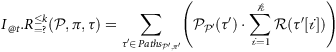 $$\small{{I}_{@ t}.R^{\leq k}_{=?}(\cal {P}, \pi, \tau ) = \& \sum _{\tau ' \in \,\it {Paths}_{\cal {P}',\pi '}} \left (P_{\cal {P}'}(\tau ')\cdot \sum _{i=\text 1}^k \cal {R}(\tau '[i])\right )}$$
where 𝒫′ = 𝒫τ[|τ|−t:] is the counterfactual MDP derived from 𝒫 and τ[|τ|−t :], i.e., the path suffix starting at the time of intervention, and π′ is the intervention policy (corresponding to π if I = $ {0/} $
). Note that the probability of ϕ is evaluated in the counterfactual model starting from the time of intervention, not from the last state of the path (to do so, one can simply replace ϕ with ℱ[t,t]ϕ). The satisfaction relation for path formulae is as follows.
$ {0/} $
). Note that the probability of ϕ is evaluated in the counterfactual model starting from the time of intervention, not from the last state of the path (to do so, one can simply replace ϕ with ℱ[t,t]ϕ). The satisfaction relation for path formulae is as follows.
Definition 7 (Semantics of PCFTL)
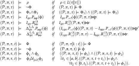
Given a PCFTL formula Φ, an MDP 𝒫, and a path τ of 𝒫 under some policy π, the PCFTL satisfaction relation ⊨ is defined by the following rules:
Remark 1. A main difference compared to existing temporal logics like PCTL⋆ is that a PCFTL formula Φ is evaluated over a path of observed states and actions rather than the current state only. Keeping track of the past allows us to perform counterfactual reasoning; see Equations 7 and 8 . Without counterfactuals, there would be no need to carry over the path, but only the current state because the system is Markovian. Footnote 5 Also, PCTL⋆ formulas evaluated over a DTMC model, while in our logic, it is convenient to keep 𝒫 and π separated rather than working with the DTMC induced by 𝒫 and π.
Remark 2. Normally, probabilistic model checking of MDPs is concerned with computing the maximum or minimum satisfaction probability across the policy space (Baier and Katoen, 2008). In this work, we instead want to compute probabilities w.r.t. given nominal and interventional/counterfactual policies, not across the entire policy space.
Building on the intuition that our counterfactual operator generalizes PCTL⋆’s probabilistic operator, we demonstrate below that our logic subsumes PCTL⋆.
Proposition 4. Every PCTL⋆ formula is a PCFTL formula, but not viceversa.
Proof. It suffices to prove that PCTL⋆’s probabilistic operator (see Baier and Katoen, 2008) is a special case of our counterfactual operator. Path formulas and their semantics are indeed equivalent between the two logics, with the only difference being that in PCFTL we keep track of the point t in the path at which ϕ is evaluated.
In particular, we show that, for s ∈ 𝒮, P
= ?(ϕ)(𝒫, π, s) = $ \emptyset $
@0.P
= ?(ϕ)(𝒫, π, (s)), where P
= ?(ϕ)(𝒫, π, s) = P
𝒫(s)({τ′ ∈ Paths
𝒫(s), π
∣(𝒫(s), π, τ′,1)⊨ϕ}) is the quantitative probabilistic operator. By applying (7), we have that
$ \emptyset $
@0.P
= ?(ϕ)(𝒫, π, (s)), where P
= ?(ϕ)(𝒫, π, s) = P
𝒫(s)({τ′ ∈ Paths
𝒫(s), π
∣(𝒫(s), π, τ′,1)⊨ϕ}) is the quantitative probabilistic operator. By applying (7), we have that
where π′ = π (the intervention is empty), and 𝒫′ = 𝒫(s). By Proposition 2, we have that 𝒫(s) = 𝒫(s).□
Expressiveness. We discuss the counterfactual operator I
@t
.P
⋈ p
(ϕ) (a similar reasoning holds for I
@t
.R
⋈ r
≤ $ {\cal k} $
). When t = 0, our operator captures the post-interventional probability; that is, the probability of a path formula ϕ after we apply intervention I at the current state. In this case, no counterfactuals need to be inferred because, trivially, we don’t have any observed MDP states beyond the time of intervention (see Figure 4b). Indeed, by Proposition 2, we have that 𝒫τ[|τ|−0:] = 𝒫(τ[|τ|−0]) = 𝒫(τ[|τ|]), that is the counterfactual MDP conditioned on the last state of τ corresponds to the original MDP 𝒫 initialized at that state. For this reason, as also shown in the proof of Propositon 4, our operator subsumes PCTL⋆’s probabilistic formula (which is indeed omitted in PCFTL): when t = 0 and I =
$ {\cal k} $
). When t = 0, our operator captures the post-interventional probability; that is, the probability of a path formula ϕ after we apply intervention I at the current state. In this case, no counterfactuals need to be inferred because, trivially, we don’t have any observed MDP states beyond the time of intervention (see Figure 4b). Indeed, by Proposition 2, we have that 𝒫τ[|τ|−0:] = 𝒫(τ[|τ|−0]) = 𝒫(τ[|τ|]), that is the counterfactual MDP conditioned on the last state of τ corresponds to the original MDP 𝒫 initialized at that state. For this reason, as also shown in the proof of Propositon 4, our operator subsumes PCTL⋆’s probabilistic formula (which is indeed omitted in PCFTL): when t = 0 and I = $ \emptyset $
, I
@t
.P
⋈ p
(ϕ) corresponds to evaluating P
⋈ p
(ϕ) w.r.t. the original MDP 𝒫 initialized at τ[|τ|−0] = τ[|τ|] and under the original policy π (see Figure 4a). Thus,
$ \emptyset $
, I
@t
.P
⋈ p
(ϕ) corresponds to evaluating P
⋈ p
(ϕ) w.r.t. the original MDP 𝒫 initialized at τ[|τ|−0] = τ[|τ|] and under the original policy π (see Figure 4a). Thus, $ \emptyset $
@0.P
⋈ p
(ϕ) ≡ P
⋈ p
(ϕ).
$ \emptyset $
@0.P
⋈ p
(ϕ) ≡ P
⋈ p
(ϕ).
When t > 0, our operator expresses a counterfactual query, which answers the question: given that we observed τ, what would have been the probability of ϕ if we had applied a particular intervention I at t steps back in the past (but under the same random circumstances that led to τ)? A common choice is to apply I at the beginning of τ (t = |τ| − 1) but other options are possible, for example intervening before some violation has happened in τ. We stress, however, that our operator goes beyond the usual notion of counterfactuals, by which the outcomes of interest are obtained only from the observed (or counterfactual) path. Indeed, depending on the bounds in the temporal operators of ϕ, evaluating ϕ might require paths that extend beyond τ. Hence, up to the length of τ, ϕ is evaluated on counterfactual paths; beyond that point, paths follow the original MDP model 𝒫 (which is precisely how our counterfactual MDP is constructed, see Def. 6) because there are no observations to condition on. We show why this matters in Example 2 below.
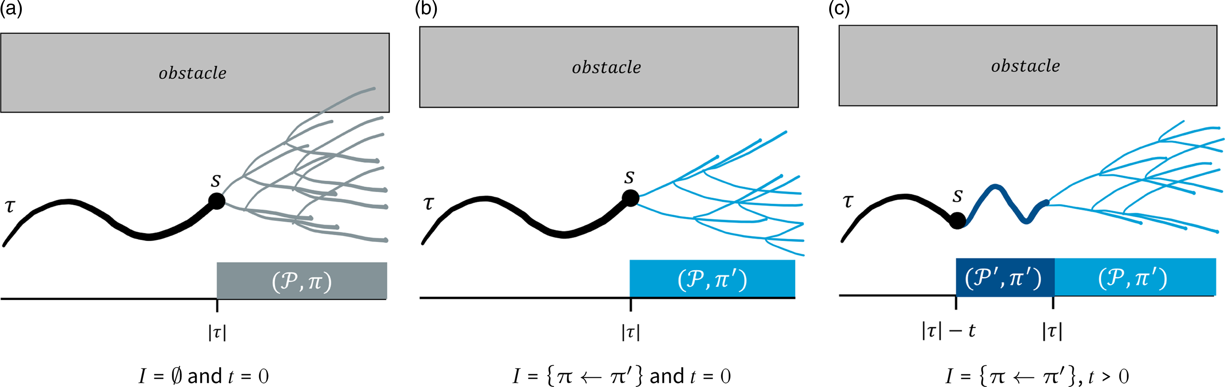
Figure 4. Three scenarios for the evaluation of I @t .P ⋈ p (ϕ). The observed path τ is in black. The counterfactual path (induced by the counterfactual MDP 𝒫′ = 𝒫τ[|τ|−t:] and the intervention policy π′) is in dark blue (in general we have a distribution of such paths, but here we show only one for simplicity). Paths extensions under the nominal policy π are in gray, and those under π′ in light blue. The horizontal axis represents time (or path positions), and the vertical axis the MDP state (continuous and one-dimensional for illustration purposes). While none of the three examples hit the obstacle within the observed/counterfactual path, moving forward, π yields a higher probability of this happening.
Example 2. Consider an MDP 𝒫 and an obstacle avoidance property φ H = 𝒢[0,H]¬obstacle for some horizon H > 0. Let τ be an observed path of 𝒫 under some policy π. Let τ I , with |τ I | = |τ|, denote the counterfactual path obtained from τ by applying some intervention I = {π ← π′} at the start. (For simplicity, we assume that only one counterfactual path is possible.) Now suppose that no obstacle is hit in τ or τ I . So, in usual counterfactual analysis, one would conclude that the nominal policy and the intervention policy are equivalent relative to property φ H and observation τ. However, if the safety property bound H extends beyond the length of τ, then it is necessary to reason about the future evolution of the MDP beyond τ (or τ I ): in one case, starting from the last state of τ and under the nominal policy; in the other, from the last state of the counterfactual path τ I and under I’s policy. At this point, it is entirely possible that going forward from the counterfactual world yields a higher probability of obstacle avoidance than remaining with the nominal policy, as illustrated in Figures 4 a and 4c. Thus, limiting the analysis to outcomes within the observed/counterfactual past, as done in previous work (Oberst and Sontag, Reference Oberst and Sontag2019; Tsirtsis, De, and Rodriguez, Reference Tsirtsis, De and Rodriguez2021), would lead to the wrong conclusion that the two policies are equivalent safety-wise.
Encoding treatment effects. We explain how the introduced causal effect operators $ \Delta_{@t}^{{I_{1}}, {I_{0}}}$
.P
⋈ p′(ϕ) and
$ \Delta_{@t}^{{I_{1}}, {I_{0}}}$
.P
⋈ p′(ϕ) and $ \Delta_{@t}^{{I_{1}}, {I_{0}}}$
.R
⋈ r
≤
$ \Delta_{@t}^{{I_{1}}, {I_{0}}}$
.R
⋈ r
≤ $ {\cal k} $
can be used to express the traditional CATE and ITE estimators (defined in Section 2.1). We saw that CATE is the difference of post-interventional probabilities, conditioned on a particular value V = v of some variable V. In reinforcement learning with MDPs, one sensible choice is to condition on the first state of the post-interventional path (Oberst and Sontag, Reference Oberst and Sontag2019). Therefore, for the same argument made above about defining post-interventional probabilities with I
@0.P
⋈ p
(ϕ) formulas, we can express this notion of CATE in PCFTL with the formula
$ {\cal k} $
can be used to express the traditional CATE and ITE estimators (defined in Section 2.1). We saw that CATE is the difference of post-interventional probabilities, conditioned on a particular value V = v of some variable V. In reinforcement learning with MDPs, one sensible choice is to condition on the first state of the post-interventional path (Oberst and Sontag, Reference Oberst and Sontag2019). Therefore, for the same argument made above about defining post-interventional probabilities with I
@0.P
⋈ p
(ϕ) formulas, we can express this notion of CATE in PCFTL with the formula $ \Delta_{@t}^{{I_{1}}, {I_{0}}}$
.P
⋈ p
(ϕ). The latter indeed is the effect in the probability of ϕ between interventions I
1 and I
0, conditioned on paths starting with τ[|τ|−0] = τ[|τ|] (the last state of τ).
$ \Delta_{@t}^{{I_{1}}, {I_{0}}}$
.P
⋈ p
(ϕ). The latter indeed is the effect in the probability of ϕ between interventions I
1 and I
0, conditioned on paths starting with τ[|τ|−0] = τ[|τ|] (the last state of τ).
ATE, the unconditional version of CATE, cannot be directly expressed in PCFTL because our semantics is defined over a non-empty path τ, and hence, probabilities are implicitly conditional on the last state τ[|τ|]. An equivalent of ATE can be defined as the expected value of the CATE formula $ \Delta_{@t}^{{I_{1}}, {I_{0}}}$
.P
⋈ p
(ϕ) evaluated at the initial states S ∼ P
I
(S) of the MDP.
$ \Delta_{@t}^{{I_{1}}, {I_{0}}}$
.P
⋈ p
(ϕ) evaluated at the initial states S ∼ P
I
(S) of the MDP.
Finally, akin to how I
@t
.P
⋈ p
(ϕ) with t > 0 expresses a counterfactual probability (as discussed previously), the operator $ \Delta_{@t}^{{I_{1}}, {I_{0}}}$
.P
⋈ p
(ϕ) with t > 0 provides a notion of ITE, because, like ITE, our operator is defined as the difference of the counterfactual probabilities I
1@t
.P
= ?(ϕ) and I
0@t
.P
= ?(ϕ).
$ \Delta_{@t}^{{I_{1}}, {I_{0}}}$
.P
⋈ p
(ϕ) with t > 0 provides a notion of ITE, because, like ITE, our operator is defined as the difference of the counterfactual probabilities I
1@t
.P
= ?(ϕ) and I
0@t
.P
= ?(ϕ).
4.1. Example properties
Below, we provide examples of useful properties that can be expressed with the newly introduced counterfactual and causal effect operators of PCFTL, for the verification of cyber-physical systems.
Example 3. Let τ denote an observed path (of length τ) in an arbitrary MDP 𝒫 under policy π. Let π′ represent an alternative policy that we can intervene on, defined by I′ = π ← π′, and let ϕ be a path formula describing some requirement of interest. Using PCFTL, we can express many interventional and counterfactual properties related to cyber-physical systems, such as:
-
Safety:
-
– I @|τ| − 1.P ≥ 0.99(𝒢[0,20]signal < threshold): ‘If we had replaced the nominal policy π with π′ at the beginning, would the probability of the signal remaining below a specified safety threshold over the next 20 steps have been at least 99%?”
-
– Δ @0 I′,
$ \emptyset $
. P > 0(𝒢[a,b]ϕ): “Is π′ safer than π moving forward from the current state (between bounds a and b)?” (this is a CATE-like query)
-
–
$ \emptyset $
@t
.P
< p
(𝒢[a,b]ϕ) → I′@t
.P
≥ p
(𝒢[a,b]ϕ): “Had we deployed π′ t steps in the past, would we have observed a safety probability of at least p if π failed to achieve so?”
-
– I′@t .P = ?(ℱ[t′,t′](¬ϕ∧Δ @0 I″,
$ \emptyset $
. P > 0 ℱ[1,H]ϕ)), where I″ = {(π←π″)} and H ≥ 1 : “What would have been the probability, had we applied π′ t steps in the past, of observing a violation after time t′, and subsequently, of a different policy π″ yielding a better recovery probability than π′?”
-
-
Liveness:
-
– I @|τ| − 1.P ≥ 0.99(𝒢[0,20]waiting_for_resource < ℱ acquired_resource): ‘If we had replaced the nominal policy π with π′ at the beginning, would the probability of avoiding resource starvation over the next 20 steps have been at least 99%?”
-
-
Reachability:
-
– I @0.P ≥ 0.95(ℱ[0,10]goal): “If we apply the intervention I′ = {(π←π′)} in the current state, will the probability of reaching the goal state(s) within 10 steps be at least 95%?”
-
– Δ @0 I′,
$ \emptyset $
. P
≥ 0(ℱ[0,10]goal): “If we replaced the nominal policy π with π′ at the current time step, would this increase the likelihood of reaching the goal state(s) within the next 10 steps?”
-
-
Reward-based properties:
-
– I @10.R ≥ 200 ≤ |τ| : “If we replaced the nominal policy π with π′ in the last 10 time steps, would the expected reward be over 200?”
-
– Δ @|τ| − 1 I′,
$ \emptyset $
. R ≥ 30 ≤ |τ|: “If we replaced the nominal policy π with π′ at the beginning, would the expected reward over τ steps under π′ have been at least 30 higher than the expected reward under π”
-


4.2. Decidability
Despite the added expressiveness, PCFTL remains decidable. First, we note that the transition probability function of a counterfactual MDP, defined in (6), is a well-defined probability measure. Therefore, the set of paths induced by a counterfactual MDP 𝒫′ and some policy is also measurable (Baier and Katoen, 2008), which ensures that we can quantify the probability of a path formula.
A decision procedure for PCFTL can be adapted from the standard model checking algorithm for a DTMC 𝒟 = (𝒮, P
𝒟, P
I
, R, L) and a PCTL* formula Φ (Baier and Katoen, 2008), which we summarise next. The procedure traverses the parse tree of Φ bottom-up. For each node, representing a subformula $ \Psi $
, the satisfaction set Sat(
$ \Psi $
, the satisfaction set Sat( $ \Psi $
) = {s ∈ 𝒮 ∣ s ⊨
$ \Psi $
) = {s ∈ 𝒮 ∣ s ⊨ $ \Psi $
} is computed. When
$ \Psi $
} is computed. When $ \Psi $
is a simple Boolean formula, computing Sat(
$ \Psi $
is a simple Boolean formula, computing Sat( $ \Psi $
) is straightforward, so we focus on the case
$ \Psi $
) is straightforward, so we focus on the case $ \Psi $
= P
⋈ p′(ϕ). Here, all maximal state subformulas of ϕ are replaced with new atomic propositions representing their satisfaction sets. This step is possible because the satisfaction sets are precomputed during the bottom-up traversal. This operation effectively transforms ϕ into an LTL property, which enables the computation of P
𝒟(s ⊨ ϕ) using a standard automata-based approach (Baier and Katoen, 2008). Hence, we can compute the satisfaction set of
$ \Psi $
= P
⋈ p′(ϕ). Here, all maximal state subformulas of ϕ are replaced with new atomic propositions representing their satisfaction sets. This step is possible because the satisfaction sets are precomputed during the bottom-up traversal. This operation effectively transforms ϕ into an LTL property, which enables the computation of P
𝒟(s ⊨ ϕ) using a standard automata-based approach (Baier and Katoen, 2008). Hence, we can compute the satisfaction set of $ \Psi $
as Sat(
$ \Psi $
as Sat( $ \Psi $
) = {s ∈ 𝒮 ∣P
𝒟(s ⊨ ϕ) ⋈ p′}.
$ \Psi $
) = {s ∈ 𝒮 ∣P
𝒟(s ⊨ ϕ) ⋈ p′}.
Model-checking PCTL* has double-exponential time complexity in |ϕ| due to the transformation of ϕ′ into a deterministic Rabin automaton and polynomial complexity in the size of the DTMC. Moreover, as demonstrated by Kwiatkowska et al. (Reference Kwiatkowska, Norman and Parker2007), determining reward properties does not impact the decidability or time complexity of the model-checking procedure, so we will not discuss this case here.
The decision procedure for PCFTL follows a similar approach. We do not discuss Boolean and reward properties and cover the case when $ \Psi $
= I
@t
.P
⋈ p
(ϕ) (from which a procedure for
$ \Psi $
= I
@t
.P
⋈ p
(ϕ) (from which a procedure for $ \Delta_{@t}^{{I_{1}}, {I_{0}}}$
.P
⋈ p′(ϕ) can be easily derived). The key difference here is that the satisfaction set for Sat(
$ \Delta_{@t}^{{I_{1}}, {I_{0}}}$
.P
⋈ p′(ϕ) can be easily derived). The key difference here is that the satisfaction set for Sat( $ \Psi $
) cannot include states, but it must include paths because the satisfaction of I
@t
.P
⋈ p
(ϕ) depends on an (observed) path. It is important to note that this set will include paths of at most length T where T is the largest t offset of an intervention appearing in any state subformula. Indeed, it is easy to see that the satisfaction of I
@t
.P
⋈ p
(ϕ) w.r.t. a path τ (with |τ| ≥ t) depends only on the t-length suffix of τ (which is the suffix used to construct the counterfactual MDP, see (7)). To transform the path formula ϕ into an equivalent LTL formula (as done above), we now need to express these satisfaction sets (defined over finite paths, i.e., sequences of states) as atomic propositions (defined over states). This is possible by augmenting the MDP with memory to keep track of the last T − 1 visited states.Footnote
6
In this way, there is a direct correspondence between the elements of Sat(
$ \Psi $
) cannot include states, but it must include paths because the satisfaction of I
@t
.P
⋈ p
(ϕ) depends on an (observed) path. It is important to note that this set will include paths of at most length T where T is the largest t offset of an intervention appearing in any state subformula. Indeed, it is easy to see that the satisfaction of I
@t
.P
⋈ p
(ϕ) w.r.t. a path τ (with |τ| ≥ t) depends only on the t-length suffix of τ (which is the suffix used to construct the counterfactual MDP, see (7)). To transform the path formula ϕ into an equivalent LTL formula (as done above), we now need to express these satisfaction sets (defined over finite paths, i.e., sequences of states) as atomic propositions (defined over states). This is possible by augmenting the MDP with memory to keep track of the last T − 1 visited states.Footnote
6
In this way, there is a direct correspondence between the elements of Sat( $ \Psi $
) and the states of the augmented MDP, as desired. So, we can now construct our sets as done for the PCTL* case above, as Sat(
$ \Psi $
) and the states of the augmented MDP, as desired. So, we can now construct our sets as done for the PCTL* case above, as Sat( $ \Psi $
) = {τ ∈ ⋃1 ≤ i ≤ T
𝒮
i
∣ P
𝒟τ, π′
(τ[1]⊨ϕ)} where 𝒟τ, π′ is the (counterfactual) DTMC induced by the interventional policy π′ and by the counterfactual MDP associated to the original MDP and path τ. Having shown that PCFTL model checking reduces to PCTL* model checking, its complexity is still polynomial in the size of the induced (counterfactual) DTMC, as the state space size of the augmented model is polynomial in that of the induced DTMC.
$ \Psi $
) = {τ ∈ ⋃1 ≤ i ≤ T
𝒮
i
∣ P
𝒟τ, π′
(τ[1]⊨ϕ)} where 𝒟τ, π′ is the (counterfactual) DTMC induced by the interventional policy π′ and by the counterfactual MDP associated to the original MDP and path τ. Having shown that PCFTL model checking reduces to PCTL* model checking, its complexity is still polynomial in the size of the induced (counterfactual) DTMC, as the state space size of the augmented model is polynomial in that of the induced DTMC.
5. PCFTL verification with statistical model checking
We use statistical model checking (SMC) (Younes and Simmons, Reference Younes and Simmons2006; Legay et al., Reference Legay, Delahaye and Bensalem2010) to determine whether our properties are satisfied, that is by sampling finite paths of the (counterfactual) MDP model. We leave the study of numerical-symbolic algorithms for future work.
Since we deal with finite paths, we consider a fragment of the logic with bounded temporal operators. Also, we restrict to non-nested properties, that is those where path sub-formulas ϕ do not contain in turn counterfactual operators (even though we allow for arbitrary nesting of temporal operators in ϕ). The complication with nested formulas is that we require multiple executions to determine the satisfaction of ϕ, leading to a sample size that is exponential in the depth of the nested operator (Younes and Simmons, Reference Younes and Simmons2006; Legay et al., Reference Legay, Delahaye and Bensalem2010). Nevertheless, the fragment we consider is rich enough to express a variety of reinforcement learning tasks (see Section 6) and subsumes Probabilistic Bounded LTL (Zuliani, Platzer, and Clarke, Reference Zuliani, Platzer and Clarke2013) (because our counterfactual formulas generalize probabilistic ones).
In short, with SMC we reduce the problem of checking I @t .P ≥ p (ϕ) to one of hypothesis testing, given a sample of MDP realizations. As in (Younes and Simmons, Reference Younes and Simmons2006; Legay et al., Reference Legay, Delahaye and Bensalem2010), we employ a sequential scheme that allows sampling only the number of paths necessary to ensure a priori probabilities α and β of type-1 errors (wrongly concluding that the property is false) and type-2 errors (wrongly concluding that it is true), respectively. Our approach builds on (Younes and Simmons, Reference Younes and Simmons2006; Legay et al., Reference Legay, Delahaye and Bensalem2010) and extends it to handle reward and causal effect properties, by defining a suitable sequential test for T-distributed outcomes (rather than Bernoulli ones as done in Younes and Simmons (Reference Younes and Simmons2006) and Legay et al. (Reference Legay, Delahaye and Bensalem2010)).
5.1. Computation of counterfactuals and causal effects
SMC relies on sampling paths of the (counterfactual) MDP model under some policy. We choose to sample these paths using the Gumbel-Max trick (see (5)) as it facilitates inference for the causal effect operator, as we will explain next. Using this formulation, we can express the counterfactual probability of (7) as the expectation of a function $f(\bf {G})$
of (prior) Gumbel variables
$f(\bf {G})$
of (prior) Gumbel variables ${\bf {G}}\sim \rm {Gumbel}$
, as follows:
${\bf {G}}\sim \rm {Gumbel}$
, as follows:
 $${I_{@ t}.P_{=?}(\rm \phi )({\it{\cal {P}}, \pi, \tau} ) = {\mathbb {E}}_{\bf {G}}[f({\bf {G}})], \text { with } \ f({\bf {G}}) = {\bf {\rm \bf 1}}({\it{\cal {P}}', \pi ', \tau '({\bf {G}})},\text 1) \models \phi ),} $$
where $\bf {1}$
is the indicator function, 𝒫′ = 𝒫τ[|τ|−t:] is the counterfactual MDP, π′ is intervention I’s policy, and
$\bf {1}$
is the indicator function, 𝒫′ = 𝒫τ[|τ|−t:] is the counterfactual MDP, π′ is intervention I’s policy, and $\tau '(\bf {G})$
is the path of 𝒫′ under π′ which is uniquely determined by
$\tau '(\bf {G})$
is the path of 𝒫′ under π′ which is uniquely determined by $\bf {G}$
.Footnote
7
$\bf {G}$
.Footnote
7
The corresponding formulation for the counterfactual reward of (8) is readily obtained as:
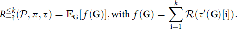 $$ R^{\leq \it k}_{=?}({\cal {P}}, \pi, \tau ) = {\mathbb {E}}_{{\bf {G}}}[\,f({\bf {G}})], \text { with } {\it \ f}({\bf {G}})=\sum _{i=1}^{\it k} {\cal {R}}(\tau '({\bf {G}})[i]). $$
We proceed similarly for causal effect operators, with one important difference. While in Definition 7, we formulated the causal effect as the difference of two independent probabilities (or expected rewards), we here express it as the mean of paired differences between individual outcomes. This will allow us to reduce a two-sample inference problem into a one-sample problem.
 $${{\Delta ^{I_1,I_0}_{@t}.P_{=?}({\rm \phi} )({\cal {P}}, \pi, \tau ): \ \ f({\bf {G}})={\bf {1}}({\cal {P}}', \pi _1, \tau _1({\bf {G}}),1) \models \phi ){}{}}{ - {\bf {1}}({\cal {P}}', \pi _0, \tau _0({\bf {G}}),\text 1) \models \phi )}}$$
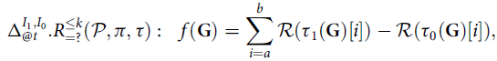 $$\Delta ^{I_1,I_0}_{@t}.R^{\leq k}_{=?}({\cal {P}}, \pi, \tau ) : \ \ f({\bf {G}})=\sum _{i=a}^b {\cal {R}}(\tau _1({\bf {G}})[i])-{\cal {R}}(\tau _0({\bf {G}})[i]),$$
where for i = 0, 1, π
i
is I
i
’s policy, and $\tau _i({\bf {G}})$
is the path of the counterfactual MDP 𝒫′ under π
i
uniquely determined by the Gumbel G. The advantage of the above form using paired differences is that this yields smaller variability, and hence, a more accurate statistical estimation, than the one based on the difference of independent means.
$\tau _i({\bf {G}})$
is the path of the counterfactual MDP 𝒫′ under π
i
uniquely determined by the Gumbel G. The advantage of the above form using paired differences is that this yields smaller variability, and hence, a more accurate statistical estimation, than the one based on the difference of independent means.
5.2. Qualitative properties
Let p ϕ = I @t .P = ?(ϕ)(𝒫,π,τ) be the true (unknown) counterfactual probability of ϕ for a given MDP 𝒫, policy π, and path τ. The problem of checking whether p ϕ is above a given threshold θ, that is deciding property I @t .P ≥ θ(ϕ), can be formulated and solved as one of hypothesis testing, where we test the hypothesis H : p ϕ ≥ θ against K : p ϕ < θ using a set of observations x 1, …, x m of the underlying process.
Hypothesis testing may incur two kinds of errors: type-1 errors, that is wrongly concluding that K is true (when H holds) and type-2 errors, that is wrongly concluding that H is true (when K holds). We denote the probability of type-1 errors by α and that of type-2 errors by β. The pair ⟨α, β⟩ is also called the strength of the test.
Wald’s sequential probability ratio test (SPRT) (Wald, Reference Wald2004) is an efficient scheme used in probabilistic model checking (Younes and Simmons, Reference Younes and Simmons2006; Younes et al., Reference Younes, Kwiatkowska, Norman and Parker2006) to sample only the number of realizations necessary to answer the above hypothesis test with strength ⟨α, β⟩. We first explain in detail the SPRT for I @t .P ≥ θ(ϕ) properties, and then briefly cover the other kinds of formulas.
I @t .P ≥ θ(ϕ) properties. The SPRT method considers the following relaxation of the original hypotheses: H 0 : p ϕ ≥ θ0 VS H 1 : p ϕ ≤ θ1, with θ0 = θ + δ and θ1 = θ − δ, where δ > 0 is a user-defined parameter. The interval (θ1,θ0) is called indifference region, as we are willing to accept either hypothesis when p ϕ ∈ (θ1,θ0). This relaxation is necessary because, when testing the original hypotheses H and K, we cannot control simultaneously both α and β if the true probability p ϕ is exactly equal to θ, see (Younes and Simmons, Reference Younes and Simmons2006; Younes et al., Reference Younes, Kwiatkowska, Norman and Parker2006).
In the SPRT, we collect observations iteratively. At the m-th iteration, we have m observations ${\bf {x}}_m = (x_1,\ldots, x_m)$
. In our case, these are counterfactual outcomes, that is realizations of the Bernoulli process (X
1, …, X
m
) where
${\bf {x}}_m = (x_1,\ldots, x_m)$
. In our case, these are counterfactual outcomes, that is realizations of the Bernoulli process (X
1, …, X
m
) where $X_i \sim f({\bf {G}})={\bf {1}}({\cal {P}}', \pi ', \tau '({\bf {G}}),1) \models \phi )$
(see Eq. 9). Given
$X_i \sim f({\bf {G}})={\bf {1}}({\cal {P}}', \pi ', \tau '({\bf {G}}),1) \models \phi )$
(see Eq. 9). Given ${\bf {x}}_m$
, we compute the following likelihood ratio (LR)
${\bf {x}}_m$
, we compute the following likelihood ratio (LR)
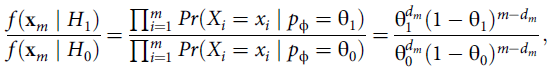 $$ {{f({\bf {x}}_m \mid H_1)} \over {f({\bf {x}}_m \mid H_0)}} = {{\prod _{i=1}^m Pr(X_i = x_i \mid p_{{\rm \phi} }= {\rm \theta} _1)}\over {\prod _{i=1}^m Pr(X_i = x_i \mid p_{{\rm \phi} }={\rm \theta} _0)}} = { {{\rm \theta} _1^{d_m}(1-{\rm \theta} _1)^{m-d_m}} \over {{\rm \theta} _0^{d_m}(1-{\rm \theta} _0)^{m-d_m}}}, $$
where $d_m=\sum _{i=1}^m x_i$
is the number of observed successes. In other words,
$d_m=\sum _{i=1}^m x_i$
is the number of observed successes. In other words, $f({\bf {x}}_m \mid H_i)$
is the probability of observing the sequence
$f({\bf {x}}_m \mid H_i)$
is the probability of observing the sequence ${\bf {x}}_m$
if p
ϕ = θ
i
holds. At this point, the SPRT compares the LR with the constants A = (1−β)/α and B = β/(1−α) and: if
${\bf {x}}_m$
if p
ϕ = θ
i
holds. At this point, the SPRT compares the LR with the constants A = (1−β)/α and B = β/(1−α) and: if ${{f({\bf {x}}_m \mid H_1)} \over {f({\bf {x}}_m \mid H_0)} }\leq B$
, we accept H
0, with a type-2 error probability of β;
${{f({\bf {x}}_m \mid H_1)} \over {f({\bf {x}}_m \mid H_0)} }\leq B$
, we accept H
0, with a type-2 error probability of β;
if ${{f({\bf {x}}_m \mid H_1)} \over {f({\bf {x}}_m \mid H_0)}}\geq A$
, we accept H
1, with a type-1 error probability of α; or,
${{f({\bf {x}}_m \mid H_1)} \over {f({\bf {x}}_m \mid H_0)}}\geq A$
, we accept H
1, with a type-1 error probability of α; or,
we collect additional observations until one of the two above conditions hold. Note that this procedure requires a larger number of observations as the true p ϕ approaches the threshold θ. Nevertheless, a decision is always reached after a finite number of steps (see Younes and Simmons (Reference Younes and Simmons2006); Younes et al. (Reference Younes, Kwiatkowska, Norman and Parker2006) for a more detailed analysis of the SPRT’s stopping time). The above decision scheme is valid for other kinds of properties as well, that is it doesn’t depend on the underlying distribution of the observations, as long as the LR is adequately defined. Hence, we won’t repeat it for the cases below.
I
@t
.R
≥ θ ≤ $ {\cal k} $
formulas. The SPRT can be also applied to variables other than Bernoulli, as are those entailed by reward-based properties. The corresponding test is an application of the SPRT to T-distributed observations (Schnuerch and Erdfelder, 2020). Let μ be the true (unknown) average cumulative reward, that is μ = I
@t
.R
= ? ≤
$ {\cal k} $
formulas. The SPRT can be also applied to variables other than Bernoulli, as are those entailed by reward-based properties. The corresponding test is an application of the SPRT to T-distributed observations (Schnuerch and Erdfelder, 2020). Let μ be the true (unknown) average cumulative reward, that is μ = I
@t
.R
= ? ≤ $ {\cal k} $
. Here, we sample observations from the
$ {\cal k} $
. Here, we sample observations from the $f({\bf {G}})$
of (10), for which we have that
$f({\bf {G}})$
of (10), for which we have that $\mu ={\mathbb {E}} [f({\bf {G}})]$
.
$\mu ={\mathbb {E}} [f({\bf {G}})]$
.
We consider the hypotheses: H
0 : μ ≥ θ0 VS H
1 : μ ≤ θ1, with θ0 = θ + δ ⋅ σ and θ1 = θ − δ ⋅ σ, where σ is the (unknown) standard deviation of $f({\bf {G}})$
, and δ > 0 is the indifference parameter: the indifference region spans 2 ⋅ δ standard deviations around θ.
$f({\bf {G}})$
, and δ > 0 is the indifference parameter: the indifference region spans 2 ⋅ δ standard deviations around θ.
The definition of the LR follows the intuition that if H
0 holds and in particular, μ = θ0, then the variable T
m
= (X̄
m
−θ)/S
m
follows a non-central T distribution with non-centrality parameter $\delta \cdot \sqrt {m}$
and m − 1 degrees of freedom, where
$\delta \cdot \sqrt {m}$
and m − 1 degrees of freedom, where $ {\bar{X}}_m= {{1}\over{m}}\sum_{i=1}^{m} X_{i}$
is the sample mean and
$ {\bar{X}}_m= {{1}\over{m}}\sum_{i=1}^{m} X_{i}$
is the sample mean and $S_m = {{1}\over {\sqrt {m}}}\sqrt { {{1}\over{m-1}} \sum _{i=1}^m (X_i - \bar {X}_m)^2}$
is the standard error of X̄
m
(Schnuerch and Erdfelder, 2020). The same reasoning holds for H
1, but after adjusting the sign of T
m
. Hence, the LR is given by
$S_m = {{1}\over {\sqrt {m}}}\sqrt { {{1}\over{m-1}} \sum _{i=1}^m (X_i - \bar {X}_m)^2}$
is the standard error of X̄
m
(Schnuerch and Erdfelder, 2020). The same reasoning holds for H
1, but after adjusting the sign of T
m
. Hence, the LR is given by $ {{f({\bf {x}}_m \mid H_1)} \over {f({\bf {x}}_m \mid H_0)} } = {{f_T(-t_m \mid m-1,\delta \cdot \sqrt {m})} \over {f_T(t_m \mid m-1,\delta \cdot \sqrt {m})}}$
where t
m
is the observed value of T
m
and
$ {{f({\bf {x}}_m \mid H_1)} \over {f({\bf {x}}_m \mid H_0)} } = {{f_T(-t_m \mid m-1,\delta \cdot \sqrt {m})} \over {f_T(t_m \mid m-1,\delta \cdot \sqrt {m})}}$
where t
m
is the observed value of T
m
and $f_T(x \mid m-1,\delta \cdot \sqrt {m})$
is the p.d.f. at x of the non-central T distribution with m − 1 degrees of freedom and parameter
$f_T(x \mid m-1,\delta \cdot \sqrt {m})$
is the p.d.f. at x of the non-central T distribution with m − 1 degrees of freedom and parameter $\delta \cdot \sqrt {m}$
.
$\delta \cdot \sqrt {m}$
. $ \Delta_{@t}^{{I_{1}}, {I_{0}}}$
.P
≥ θ(ϕ) and
$ \Delta_{@t}^{{I_{1}}, {I_{0}}}$
.P
≥ θ(ϕ) and $ \Delta_{@t}^{{I_{1}}, {I_{0}}}$
.R
≥ θ ≤
$ \Delta_{@t}^{{I_{1}}, {I_{0}}}$
.R
≥ θ ≤ $ {\cal k} $
formulas. Since we can express the causal effect as the mean of a (non-Bernoulli) variable (the paired difference in the counterfactual outcomes of I
1 and I
0), we can apply the same SPRT procedure introduced above for I
@t
.R
≥ θ ≤
$ {\cal k} $
formulas. Since we can express the causal effect as the mean of a (non-Bernoulli) variable (the paired difference in the counterfactual outcomes of I
1 and I
0), we can apply the same SPRT procedure introduced above for I
@t
.R
≥ θ ≤ $ {\cal k} $
formulas,Footnote
8
provided that we use the correct definition of
$ {\cal k} $
formulas,Footnote
8
provided that we use the correct definition of $f(\bf {G})$
, that is that of (11) for
$f(\bf {G})$
, that is that of (11) for $ \Delta_{@t}^{{I_{1}}, {I_{0}}}$
.P
≥ θ(ϕ) and (12) for
$ \Delta_{@t}^{{I_{1}}, {I_{0}}}$
.P
≥ θ(ϕ) and (12) for $ \Delta_{@t}^{{I_{1}}, {I_{0}}}$
.R
≥ θ ≤
$ \Delta_{@t}^{{I_{1}}, {I_{0}}}$
.R
≥ θ ≤ $ {\cal k} $
.
$ {\cal k} $
.
When I 1 = I 0, however, the above procedure fails because the two policies attain the same outcomes, and so their pairwise differences are constantly 0, resulting in S m = 0 and T m = ∞, which has a likelihood of 0. To detect this case, as done in David et al. (Reference David, Larsen, Legay, Mikucionis, Poulsen, Van Vliet and Wang2011), we run a dedicated SPRT to test that the probability of obtaining equal outcomes is equal to 1.
Boolean combinations. To verify ¬Φ with strength ⟨α, β⟩, we verify Φ with strength ⟨β, α⟩ and negate the result. To verify a conjunction $\bigwedge _{i=1}^N \Phi _i$
with strength ⟨α, β⟩, we need to verify each conjunct Φ
i
with strength ⟨α/N, β⟩. See (Younes and Simmons, Reference Younes and Simmons2006) for more details.
$\bigwedge _{i=1}^N \Phi _i$
with strength ⟨α, β⟩, we need to verify each conjunct Φ
i
with strength ⟨α/N, β⟩. See (Younes and Simmons, Reference Younes and Simmons2006) for more details.
5.3. Quantitative properties
For quantitative properties, we use Chernoff-Hoeffding bounds to identify the number of realizations n necessary such that the Monte-Carlo estimate of the probability (or reward) property meets a priori error and confidence bounds. Given an error bound δ > 0 and an iid sample X
1, …, X
n
such that for each i = 1, …, n, 𝔼[X
i
] = μ and x
l
≤ X
i
≤ x
u
for some constant x
l
< x
u
, then the Hoeffding inequality (Hoeffding, Reference Hoeffding1963) establishes that $P(| \ {\bar{X}_n - \mu | \geq \delta )\leq 2\exp \left (- {{2n\delta ^2}\over{(x_u-x_l)^2}}\right )},$
where
$P(| \ {\bar{X}_n - \mu | \geq \delta )\leq 2\exp \left (- {{2n\delta ^2}\over{(x_u-x_l)^2}}\right )},$
where $\bar{X}_n=(1/n) \sum _{i=1}^n X_i$
is the sample mean. Hence, given bounds δ > 0 and 0 < α < 1, one can determine a priori the number of realizations n such that P(|X̄
n
−μ| ≥ δ) ≤ α, by equating
$\bar{X}_n=(1/n) \sum _{i=1}^n X_i$
is the sample mean. Hence, given bounds δ > 0 and 0 < α < 1, one can determine a priori the number of realizations n such that P(|X̄
n
−μ| ≥ δ) ≤ α, by equating $\alpha =2\exp {\left (-{{2n\delta ^2}\over {(x_u-x_l)^2}}\right )}$
and obtaining
$\alpha =2\exp {\left (-{{2n\delta ^2}\over {(x_u-x_l)^2}}\right )}$
and obtaining $ n = \left \lceil - {{(x_u-x_l)^2\log {(\alpha /2)}} \over {2\delta ^2}} \right \rceil$
.
$ n = \left \lceil - {{(x_u-x_l)^2\log {(\alpha /2)}} \over {2\delta ^2}} \right \rceil$
.
For the special case of I
@t
.P
= ?(ϕ) properties, X̄
n
is the sample estimate of the probability, μ is the probability to estimate (and hence 0 < δ < 1), x
l
= 0 and x
u
= 1. For $ \Delta_{@t}^{{I_{1}}, {I_{0}}}$
.P
= ?(ϕ) properties, we have that x
l
= − 1 and x
u
= 1 as these are the ranges for the difference of two Bernoulli outcomes. For I
@t
.R
= ? ≤
$ \Delta_{@t}^{{I_{1}}, {I_{0}}}$
.P
= ?(ϕ) properties, we have that x
l
= − 1 and x
u
= 1 as these are the ranges for the difference of two Bernoulli outcomes. For I
@t
.R
= ? ≤ $ {\cal k} $
formulas, each realization is a cumulative reward value, hence x
l
=
$ {\cal k} $
formulas, each realization is a cumulative reward value, hence x
l
= $ {\cal k} $
⋅ ℛ
l
and x
u
=
$ {\cal k} $
⋅ ℛ
l
and x
u
= $ {\cal k} $
⋅ ℛ
u
where ℛ
u
and ℛ
l
are, respectively, the largest and smallest values of the MDP’s reward function ℛ. Hence, for
$ {\cal k} $
⋅ ℛ
u
where ℛ
u
and ℛ
l
are, respectively, the largest and smallest values of the MDP’s reward function ℛ. Hence, for $ \Delta_{@t}^{{I_{1}}, {I_{0}}}$
.R
= ? ≤
$ \Delta_{@t}^{{I_{1}}, {I_{0}}}$
.R
= ? ≤ $ {\cal k} $
formulas, we have x
u
=
$ {\cal k} $
formulas, we have x
u
= $ {\cal k} $
(ℛ
u
−ℛ
l
) and x
l
=
$ {\cal k} $
(ℛ
u
−ℛ
l
) and x
l
= $ {\cal k} $
(ℛ
l
−ℛ
u
).
$ {\cal k} $
(ℛ
l
−ℛ
u
).
These a priori bounds, however, might be too conservative, especially for reward properties where the range (x u −x l ) tends to be consistently larger than what observed empirically. An alternative is to compute confidence intervals, that is fix the sample size n and the confidence 1 − α, thereby obtaining an estimate X̄ n and an interval [X̄ n ]α ∋ X̄ n such that P(μ ∉[X̄ n ]α) = α. In this sense, the width of [X̄ n ]α is comparable to the δ bound in Hoeffding inequality. To construct confidence intervals for I @t .P = ?(ϕ) properties, one can use the common normal-approximation (aka Wald) interval if n is not too small or the true probability not too close to 0 or 1,Footnote 9 or use the ‘exact” (but usually conservative) Clopper-Pearson interval. For the other properties, we can construct one-sample mean intervals using the T distribution.
5.4. Algorithmic complexity
The complexity of SMC is O( $ {\cal k} $
⋅N⋅c
ϕ) where
$ {\cal k} $
⋅N⋅c
ϕ) where $ {\cal k} $
is the number of counterfactual operators in the formula, N is the number of sampled paths (for each operator), and c
ϕ is the cost of evaluating the operator’s path formula ϕ on each path. The latter term has complexity O((2|τ|)
d
) where |τ| is the path length (bounded by the temporal bounds in ϕ) and d is the depth of ϕ, that is the maximum number of nested until expressions (Bartocci et al., Reference Bartocci, Ferrère, Manjunath and Nickovic2018). The term N is a random variable (owing to the randomness of the sample) and its expected value depends on the true (unknown) probability p to evaluate and the error bounds α and β. Formulas for 𝔼[N] can be found for specific values of p, see (Younes and Simmons, Reference Younes and Simmons2006), but no general analytical form exists. Nevertheless, the SMC algorithm terminates with probability 1 (Younes and Simmons, Reference Younes and Simmons2006).
$ {\cal k} $
is the number of counterfactual operators in the formula, N is the number of sampled paths (for each operator), and c
ϕ is the cost of evaluating the operator’s path formula ϕ on each path. The latter term has complexity O((2|τ|)
d
) where |τ| is the path length (bounded by the temporal bounds in ϕ) and d is the depth of ϕ, that is the maximum number of nested until expressions (Bartocci et al., Reference Bartocci, Ferrère, Manjunath and Nickovic2018). The term N is a random variable (owing to the randomness of the sample) and its expected value depends on the true (unknown) probability p to evaluate and the error bounds α and β. Formulas for 𝔼[N] can be found for specific values of p, see (Younes and Simmons, Reference Younes and Simmons2006), but no general analytical form exists. Nevertheless, the SMC algorithm terminates with probability 1 (Younes and Simmons, Reference Younes and Simmons2006).
6. Experimental evaluation
We provide two sets of results. In the first one, we consider a simple grid-world model and a reach-avoid specification. We use this case study to provide a detailed analysis of interventional and counterfactual probabilities, their variability, and the accuracy of counterfactual inference. In the second set of results, we use PCFTL on four complex 2D grid-world environments from the MiniGrid library (Chevalier-Boisvert et al., Reference Chevalier-Boisvert, Willems and Pal2018). Although these two case studies evaluate our approach on relatively similar GridWorld MDPs, we can still explore a wide range of logical specifications and properties within these environments.
6.1. Reach-avoid example
We consider a 4 × 4 grid-world example, where the agent can move up, down, left, or right, one square at a time. The specification ϕ is one of reach-avoid: we want to reach some goal region while avoiding an unsafe region, that is ϕ ≡ ¬unsafe 𝒰[0,T]goal. We choose T = 10. We consider two policies, a nominal (default) policy π and an optimal policy π o . The optimal policy is found by value iteration after assigning a reward 1 to the goal and making the unsafe and goal states terminal. The nominal policy is defined manually to make it intentionally less safe than π o . The stochasticity comes from the fact that the environment, with small probability (0.1 in our experiments), randomly takes the agent to a different position than that determined by the policy.
For each experiment in this subsection, we perform 1000 repetitions to evaluate the variability of the estimates. For each repetition, we generate 100 observed paths under the nominal policy. Counterfactuals are estimated using 20 posterior Gumbel realizations. Probability values are computed by averaging the satisfaction value of ϕ over all paths within each repetition. We choose the optimal policy as the interventional/counterfactual one, by defining I = {π ← π o }.
We evaluate the performance of the optimal policy in a counterfactual setting. In particular, we compare the probability P = ?(ϕ) under the nominal MDP against the average counterfactual probability I @t .P = ?(ϕ) for some t (where the average is w.r.t. the set of nominal paths used for P = ?(ϕ)). We apply I at the beginning of the path (t = |τ| − 1, see Figure 5a) and after the first step (t = |τ| − 2, see Figure 5b). Since π o (blue histograms in Figure 5) is safer than π (orange), the distribution of counterfactual probabilities clearly dominates that under nominal settings. See Figure 5a. For the same reason, delaying the intervention of one step leads to more unsafe trajectories (the blue histogram in Figure 5b is indeed shifted to the left compared to that in Figure 5a).
In Figure 5a, we provide results of a query corresponding to the scenario of Figure 4c, that is involving both the counterfactual past and the subsequent future evolution of the system. To do so, we draw paths τ under π of length 2 (shorter than than ϕ’s time bound) and apply I after the first time step. This results in paths that are counterfactual in the first part (because we apply I in the past, conditioned by τ) and post-interventional in the second part (because to evaluate ϕ, we need paths longer than the observed τ).
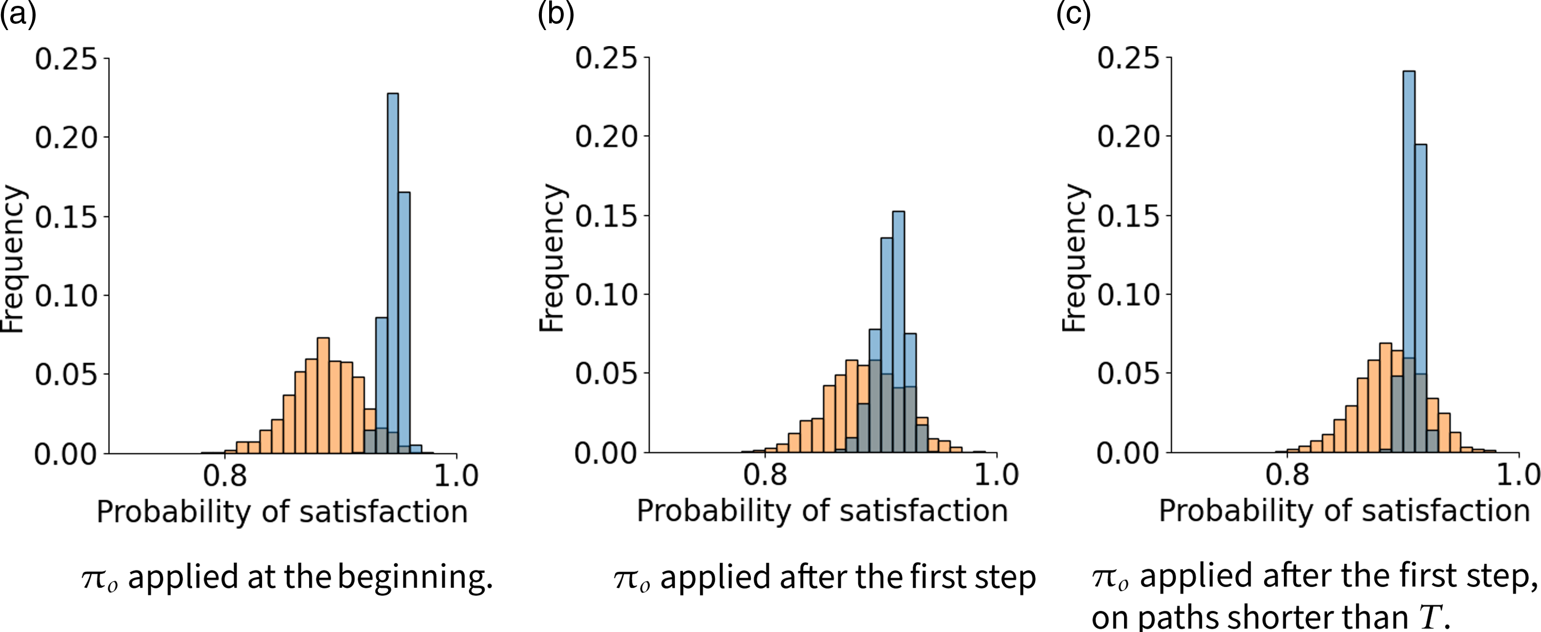
Figure 5. Counterfactual probabilities under the optimal policy π o (blue) given that we observe MDP paths under the nominal policy π (orange). In (a) and (b) paths have length 10 (same as the time bound T in ϕ). In (c), we observe paths of length 2 < T, and so, applying π o results in paths that are part counterfactual, part post-interventional.
6.2. MiniGrid benchmark
MiniGrid (Chevalier-Boisvert et al., Reference Chevalier-Boisvert, Willems and Pal2018) is a collection of 2D grid-world environments with goal-oriented tasks designed for developing reinforcement learning algorithms. Each cell in this grid world is encoded as a three-dimensional tuple (object, color, state). There are 8 different objects, 6 colors and 3 states: open, close and locked. There are 7 actions that the agent can take which are turn left, turn right, move forward, pick up, drop, toggle and done. We consider four of these environments: Empty, DoorKey, GoToDoor and Fetch.
Empty is the simplest environment, where the agent simply navigates the grid to reach some goal. This corresponds to the specification ℱ[1,T]goal, where we choose T = 50. In the DoorKey environment, a key and a door exist on the grid. The agent must first find the key, unlock the door, and reach the goal, expressed as ϕ ≡ ℱ[1,T
k
]
(key ∧ ℱ[1,T
d
]
(door ∧ ℱ[1,T
g
]
goal)), with T $ {\cal k} $
+ T
d
+ T
g
= T. This task requires the agent to learn basic navigation skills and non-trivial sequential plans. In GoToDoor, we have four doors with different colors, and the agent is tasked to reach the door of some given color: ϕ ≡ ℱ[1,T]door. The door is always unlocked, making it a simpler task than DoorKey. In Fetch, the grid contains multiple objects with assorted colors which the agent must pick up and bring to the goal: ϕ ≡ ℱ[1,T
o
]
(object∧𝒳(carrying 𝒰[1,T
g
]
goal)), with T
o
+ T
g
+ 1 = T. This task requires learning to manipulate objects and navigate the grid.
$ {\cal k} $
+ T
d
+ T
g
= T. This task requires the agent to learn basic navigation skills and non-trivial sequential plans. In GoToDoor, we have four doors with different colors, and the agent is tasked to reach the door of some given color: ϕ ≡ ℱ[1,T]door. The door is always unlocked, making it a simpler task than DoorKey. In Fetch, the grid contains multiple objects with assorted colors which the agent must pick up and bring to the goal: ϕ ≡ ℱ[1,T
o
]
(object∧𝒳(carrying 𝒰[1,T
g
]
goal)), with T
o
+ T
g
+ 1 = T. This task requires learning to manipulate objects and navigate the grid.
For each environment, we train two convolutional neural network policies using the Proximal Policy Optimization (PPO) (Schulman et al., Reference Schulman, Wolski, Dhariwal, Radford and Klimov2017) algorithm. For the nominal policy π, this time we use an optimal policy, trained using 10 million time steps. The interventional/counterfactual policy is intentionally undertrained, using only 200 time steps.
Experimental results are presented in Table 1. We examine probabilities under the nominal/optimal policy (3rd column) using the formula P ≥ 0.9(ϕ), counterfactual probabilities with the undertrained policy (4th column) using I @t .P ≥ 0.9(ϕ), and determine the causal effect between the two (5th column) using Δ @t I, Ø.P > 0(ϕ). For every environment and PCFTL formula, we carry out two set of experiments using two different intervention points, at the start of the trajectory (t = T − 1), and 10 steps into the trajectory (t = T − 11).
Table 1. PCFTL verification of the MiniGrid benchmark, with 6 x 6 grids. For each environment, we apply the intervention at the start of the path (t = T − 1) and 10 steps after the start (t = T − 11). T = 50 is the length of the path. The SMC parameters (see Section 5) are δ = 0.02, and α = 0.05 and β = 0.2 for P and I
@t
.P properties, and α = 0.01 and β = 0.2 for $ \Delta_{@t}^{{I, \emptyset}}$
.P. ⊤ and ⊥ indicate whether the SMC procedure returns true or false for the given PCFTL formulae, and in parentheses are the number of realizations required by SMC to reach this verdict
$ \Delta_{@t}^{{I, \emptyset}}$
.P. ⊤ and ⊥ indicate whether the SMC procedure returns true or false for the given PCFTL formulae, and in parentheses are the number of realizations required by SMC to reach this verdict
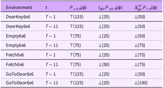
Verification results are computed using statistical model checking (see 5 for details on the decision procedures). Results indicate that the system does not satisfy the property when using an undertrained policy, while the optimal policy is always successful. This performance gap can also be seen in the causal effect column. We observe that the verification procedure is very efficient (requiring at most 125 realizations), and that the number of realizations necessary to obtain a positive answer for the nominal policy is higher than those for a negative answer for the interventional policy. The reason is that we set a high probability threshold, p ≥ 0.9, and so, even with a well-trained policy, we require a fair amount of evidence to conclude that the property is satisfied. Conversely, the interventional policy performs enough badly to require much fewer points for concluding that the property is violated.
7. Related work
Causality and verification. Concepts of causality have been investigated in formal verification for years (Baier et al., Reference Baier, Dubslaff, Funke, Jantsch, Majumdar, Piribauer and Ziemek2021). Two main classes of approaches exist, respectively based on the theory of actual causality (Halpern, Reference Halpern2016; Halpern and Pearl, Reference Halpern and Pearl2020) and on probabilistic causation. Given an SCM ℳ and a context $\mathbf {u}$
, an actual cause is, informally, the smallest set of SCM variables that, if forced with a different value, lead to a different (counterfactual) outcome for some target variable Y. This notion has been adapted in Beer et al. (2012) to find so-called root causes in LTL counterexample traces, in Gössler and Aştefǎnoaei Reference Gössler and Astefanoaei(2014) to identify the components of a timed-automata network responsible for a given failure trace, and in Leitner-Fischer and Leue (Reference Leitner-Fischer and Leue2013) to derive fault trees from probabilistic counterexamples. We note there also exist techniques not based on actual causality for finding root causes of failure in temporal logic monitoring (e.g., Bartocci et al., Reference Bartocci, Deshmukh, Donzé, Fainekos, Maler, Nickovic and Sankaranarayanan2018; Zhang et al., Reference Zhang, An, Arcaini and Hasuo2023). Probabilistic causation methods like (Baier et al., Reference Baier, Funke, Jantsch, Piribauer and Ziemek2021; Kleinberg and Mishra, Reference Kleinberg and Mishra2009; Kleinberg, Reference Kleinberg2011; Baier et al., 2022) build on the probability-raising (PR) principle by which the probability of an effect E is higher after observing a cause C than if the cause had not happened. More precisely, these works consider Markov models and express E and C as sets of states or PCTL state formulas. Our work complements these methods as it focuses not on identifying causes given some observations but on reasoning about the probability of a temporal logic specification in interventional and counterfactual settings. Methods based on actual causality similarly rely on counterfactuals but consider only non-probabilistic models. Methods based on the PR principle support probabilistic models but do not support counterfactual analysis.
$\mathbf {u}$
, an actual cause is, informally, the smallest set of SCM variables that, if forced with a different value, lead to a different (counterfactual) outcome for some target variable Y. This notion has been adapted in Beer et al. (2012) to find so-called root causes in LTL counterexample traces, in Gössler and Aştefǎnoaei Reference Gössler and Astefanoaei(2014) to identify the components of a timed-automata network responsible for a given failure trace, and in Leitner-Fischer and Leue (Reference Leitner-Fischer and Leue2013) to derive fault trees from probabilistic counterexamples. We note there also exist techniques not based on actual causality for finding root causes of failure in temporal logic monitoring (e.g., Bartocci et al., Reference Bartocci, Deshmukh, Donzé, Fainekos, Maler, Nickovic and Sankaranarayanan2018; Zhang et al., Reference Zhang, An, Arcaini and Hasuo2023). Probabilistic causation methods like (Baier et al., Reference Baier, Funke, Jantsch, Piribauer and Ziemek2021; Kleinberg and Mishra, Reference Kleinberg and Mishra2009; Kleinberg, Reference Kleinberg2011; Baier et al., 2022) build on the probability-raising (PR) principle by which the probability of an effect E is higher after observing a cause C than if the cause had not happened. More precisely, these works consider Markov models and express E and C as sets of states or PCTL state formulas. Our work complements these methods as it focuses not on identifying causes given some observations but on reasoning about the probability of a temporal logic specification in interventional and counterfactual settings. Methods based on actual causality similarly rely on counterfactuals but consider only non-probabilistic models. Methods based on the PR principle support probabilistic models but do not support counterfactual analysis.
Two relevant papers have been published in the last year at the intersection between causality and temporal logic (TL). In Coenen et al. (Reference Coenen, Finkbeiner, Frenkel, Hahn, Metzger and Siber2022), the authors extend actual causality to the case where causes and effects are given as TL properties. Their work is different from ours in that they do not consider probabilistic systems, plus they use TL to specify causes and effects, but the logic itself cannot express counterfactual queries. The work closest to ours is (Finkbeiner and Siber, Reference Finkbeiner and Siber2023), which introduces a new (non-probabilistic) counterfactual TL with would and might modalities, borrowed from Lewis’ theory of counterfactuals (Lewis, Reference Lewis2013). However, their method is model-agnostic, that is counterfactuals are obtained by manipulating the observed trace, regardless of the model that generated it. Our counterfactual traces are instead obtained by intervening on the data-generating model.
Probabilistic hyperproperties. Probabilistic hyper-properties (PHPs) for MDPs have been recently introduced in (Dimitrova et al., Reference Dimitrova, Finkbeiner and Torfah2020; Ábrahám et al., 2020) to support quantification over MDP schedulers (i.e., policies). One can see that PHPs for MDPs are strictly more expressive than the fragment of PCFTL without counterfactuals (i.e., where interventions can be applied only at t = 0). For instance, the PCFTL causal-effect formula $ \Delta_{@t}^{{I_{1}}, {I_{0}}}$
.P
⋈ p
(ϕ) can be expressed as the PHP ∃σ
1∃σ
0.P(ϕ
σ
1
) − P(ϕ
σ
0
) ⋈ p (using the syntax of (Dimitrova et al., Reference Dimitrova, Finkbeiner and Torfah2020)) where the domains of schedulers σ
0 and σ
1 are singletons (and chosen to be consistent with I
0 and I
1, respectively). However, PHPs do not support counterfactuals, which is the main strength of our method.
$ \Delta_{@t}^{{I_{1}}, {I_{0}}}$
.P
⋈ p
(ϕ) can be expressed as the PHP ∃σ
1∃σ
0.P(ϕ
σ
1
) − P(ϕ
σ
0
) ⋈ p (using the syntax of (Dimitrova et al., Reference Dimitrova, Finkbeiner and Torfah2020)) where the domains of schedulers σ
0 and σ
1 are singletons (and chosen to be consistent with I
0 and I
1, respectively). However, PHPs do not support counterfactuals, which is the main strength of our method.
Causality in reinforcement learning. There is a growing interest in applying causal inference in RL, for instance, to evaluate counterfactual policies from observational data (Oberst and Sontag, Reference Oberst and Sontag2019), provide counterfactual explanations (Tsirtsis, De, and Rodriguez, Reference Tsirtsis, De and Rodriguez2021) (i.e., the minimum number of policy actions to change in order to attain a better outcome), produce counterfactual data to enhance training of RL policies (Forney et al., Reference Forney, Pearl and Bareinboim2017; Buesing et al., Reference Buesing, Weber, Zwols, Heess, Racaniere, Guez and Lespiau2018), or estimate causal effects in presence of confounding factors (Lu, Schölkopf, and Hernández-Lobato, Reference Lu, Schölkopf and Hernández-Lobato2018). These works are very relevant yet they consider different problems from ours. That said, PCFTL builds on (Oberst and Sontag, Reference Oberst and Sontag2019) which introduces Gumbel-Max SCMs and their counterfactual stability. More recently, other methods have shown that the Gumbel-Max SCM is not the only causal model that satisfies the counterfactual stability property, and instead bound over all models that satisfy counterfactual stability (Haugh and Singal, Reference Haugh and Singal2023), or search for a particular model that optimises some given criteria (Lorberbom et al., Reference Lorberbom, Johnson, Maddison, Tarlow and Hazan2021). In this paper, we limit our attention to only Gumbel-Max SCMs since other methods are either computationally inefficient or require extra assumptions.
8. Conclusion
We have presented the probabilistic temporal logic PCFTL, the first of its kind to enable causal reasoning about interventions, counterfactuals, and causal effects in Markov Decision Processes. From a syntactic viewpoint, this is achieved by introducing an operator that subsumes interventions, counterfactuals, and the traditional probabilistic operator. The semantics of PCFTL makes use of counterfactual MDPs constructed from Gumbel-Max structural causal models, which provide a representation of discrete-state MDPs amenable to counterfactual reasoning. We performed a set of experiments on a benchmark of grid-world models, demonstrating the usefulness of the approach (being applicable to deep reinforcement learning policies as well) and the accuracy of counterfactual inference. We envision several future directions for this work, including investigating numerical or symbolic (as opposed to statistical) model-checking algorithms, and extending our approach to a broader range of systems, such as uncertain, partially observable, and continuous-time and continuous-state MDPs. Achieving this will require developing robust counterfactual inference methods tailored to these different complex systems but will ultimately enable PCFTL to be applied more broadly across a diverse set of cyber-physical and data-driven systems.
Data availability
The code for running the experiments is publicly available on Zenodo at https://doi.org/10.5281/zenodo.10619287.
Credit authorship contribution
Milad Kazemi: Formal analysis, Investigation, Methodology, Software, Validation, Visualizations, Writing. Jessica Lally: Formal analysis, Methodology, Visualizations, Writing. Nicola Paoletti: Conceptualization, Formal analysis, Funding acquisition, Methodology, Resources, Supervision, Writing.
Financial support
This work was supported by UK Research and Innovation [grant number EP/W014785/2]; and UK Research and Innovation [grant number EP/S023356/1] in the UKRI Centre for Doctoral Training in Safe and Trusted Artificial Intelligence (www.safeandtrustedai.org).
Competing interests
None.
Ethics statement
Ethical approval and consent are not relevant to this paper.


 Open access
Comments
No accompanying comment.