


Highlights
What is already known
Network meta-analysis (NMA) methods that do not rely on the proportional hazard assumption (for time-to-event outcomes) are often required in oncology. Individual event and censor times from clinical trials can typically be reconstructed from published Kaplan–Meier curves, but existing NMA methods used to synthesize these trials do not directly leverage this individual-level data.
What is new
We propose using a one-step fully Bayesian parametric NMA model that leverages individual event and censor times with the exact likelihood and allows for time-varying treatment effects. By using the exact likelihood specification, this model offers a flexible fit while avoiding certain assumptions/approximations required with existing approaches. The Bayesian framework ensures that model selection and interpretation is straightforward and efficient computation for fitting the model can be done using Stan software.
Potential impact for RSM readers outside the authors’ field
Flexible NMA methods are particularly important when there are differences in the survival distributions for the different treatments being compared, and relative treatment effects need to be extrapolated beyond the available trial data for a cost-effectiveness analysis. In this context, the one-step parametric NMA model offers a valuable tool that leverages individual-level data.
1 Introduction
Network meta-analysis (NMA) is a widely used statistical technique that expands upon standard pairwise meta-analysis, enabling simultaneous direct and indirect comparisons of multiple interventions within a unified statistical model.Reference Ades1– Reference Lu and Ades3 Given that randomized controlled trials (RCTs) in oncology rarely compare the new intervention to all relevant comparators, NMAs are often needed to synthesize time-to-event outcomes (TTE), such as progression-free survival (PFS) and overall survival (OS).Reference Ades, Welton, Dias, Phillippo and Caldwell4
The synthesis of TTE outcomes is typically based on hazard ratios (HRs)Reference Fay and Li5 derived from the Cox proportional hazards (PH) model.Reference Williamson, Smith, Hutton and Marson6, Reference Batson, Greenall and Hudson7 However, for many reasons, the PH assumption may be implausible,Reference Li, Han, Hou, Chen and Chen8– Reference Royston and Parmar10 for example, due to treatment effects that vary over time, treatment crossover, delayed treatment effects, competing risks, time-varying covariates, and differential dropout.Reference Magirr11– Reference Rahman, Fell and Ventz13 When the PH assumption does not hold, NMAs that rely on trial-specific HRs may yield biased estimates that result in poor predictions,Reference Cope, Chan and Campbell14 which are important for cost-effectiveness modeling.
Several methods have been proposed as alternatives to NMAs based on reported HRs, which have been reviewed by Cope et al.Reference Cope, Chan and Campbell14 Crowther et al.Reference Crowther, Riley, Staessen, Wang, Gueyffier and Lambert15 proposed a model for individual patient data (IPD) meta-analysis using Poisson regression models that allows for non-proportional hazards by prespecifying specific time-points at which the HR between two treatments is allowed to change. Freeman and CarpenterReference Freeman and Carpenter16 proposed NMA models using cubic splines to model the log-cumulative hazard functions. While flexible, these cubic spline models are restricted to HRs that specifically vary with log-time. Another possibility, proposed by Petit et al.Reference Petit, Blanchard, Pignon and Lueza17 is to consider the difference in restricted mean survival time at a prespecified time horizon as an alternative to the HR and to fit a standard univariate NMA. While practical, prespecifying the time horizon of interest in accordance with clinical interest may be challenging.
Ouwens et al.Reference Ouwens, Philips and Jansen18 and JansenReference Jansen19 proposed using multivariate parametric NMA models that allow for the HR to change over time. A single parametric survival distribution is used to model interventions in each trial with multivariate relative treatment effects, which are pooled and indirectly compared across trials. This means that interventions can impact both the shape and scale of a selected distribution, resulting in a time-varying treatment effect, which improves model fit and predictions. However, these models were proposed prior to the development of an algorithm to reconstruct event and censor times from the published Kaplan–Meier (KM) curves.Reference Guyot, Ades, Ouwens and Welton20 Consequently, they derived discrete hazards from “binned” events over time assuming a binomial likelihood per interval, which may be less accurate than assuming the actual event and censor times follow the likelihood for a particular distribution. Moreover, parameters for these models were transformed to a linear scale, and as a consequence, implementation of these models can be challenging given that the parameterization does not align with standard software (i.e., flexsurv in R).Reference Salanti21
To address these limitations, Cope et al.Reference Cope, Chan and Jansen22 proposed a two-step NMA approach, first fitting parametric survival distributions using frequentist maximum likelihood estimation to each arm of each trial (using the flexsurv R packageReference Jackson23). In the second step, the arm-specific parameter estimates, their standard errors, and the correlation between the parameters were synthesized using a Bayesian multivariate Normal NMA.Reference Achana, Cooper and Bujkiewicz24
Burke et al.Reference Burke, Ensor and Riley25 and Debray et al.Reference Debray, Moons, Abo-Zaid, Koffijberg and Riley26 discuss the pros and cons of two-step approaches for IPD meta-analysis relative to one-step approaches. Specifically, the two-step approach for NMA by Cope et al.Reference Cope, Chan and Jansen22 offers practical benefits in terms of using established statistical software packages and possibly improving computational burden.Reference Cope, Chan and Campbell14, Reference Freeman, Cooper, Sutton, Crowther, Carpenter and Hawkins27 However, it was only applied to a subset of relevant standard distributions (Weibull, Gompertz, log-normal, and log-logistic), with parameters transformed to be on a linear scale as in Ouwens et al.Reference Ouwens, Philips and Jansen18 It also relies on bootstrapping to account for parameter correlationReference Debray, Moons, Abo-Zaid, Koffijberg and Riley26, Reference Kanters, Karim, Thorlund, Anis and Bansback28 and requires assumptions regarding within-study normality and variance.Reference Burke, Ensor and Riley25, Reference Jackson and White29 Given that these assumptions can result in certain unexpected biases, Jackson and WhiteReference Jackson and White29 recommend that, when possible, to use one-step methods that make fewer normality assumptions. Therefore, there is a need for one-step NMA models with time-varying treatment effects that can also be applied to distributions such as gamma and generalized gamma that relate the available IPD (whether available or reconstructed) directly to the likelihoods of interest without complex reparameterizations.
In this article, a one-step parametric IPD-NMA framework for TTE outcomes is proposed, which allows for time-varying (i.e., multivariate) treatment effects with the exact likelihood. In Section 2, we extend existing one-step PH models (exponential, Weibull, and Gompertz) or accelerated failure time models (Weibull, log-logistic, gamma, log-normal, and generalized gamma)Reference Freeman, Cooper, Sutton, Crowther, Carpenter and Hawkins27, Reference Saramago, Chuang and Soares30, Reference Phillippo31 to have time-varying treatment effects. In Section 3, we evaluate the proposed method in a simulation study, and in Section 4, we apply the model to a network of RCTs evaluating multiple interventions for advanced melanoma regarding OS. We conclude in Section 5 with a general discussion, where we explain that proposed models provide the foundation for extensions to the multilevel network meta-regression (ML-NMR) framework to synthesize IPD and aggregate data (AD), while adjusting for potential prognostic factors and effect modifiers.Reference Phillippo31
2 A parametric IPD-NMA model for TTE outcomes
We follow the parametrization used by PhillippoReference Phillippo31 and adopt the reference treatment parameterization defining ${t}_{ijk}$
and
${t}_{ijk}$
and ${y}_{ijk}$
as the event time and censoring indicator, respectively, of individual i, in study j, with treatment k, for i in 1,…,N, for j in 1,…,J, and for k in 1,…,K. Importantly, k = 1 is considered the “reference treatment.” We outline the logic and formulas for the Weibull, which can be extended to other standard distributions.
${y}_{ijk}$
as the event time and censoring indicator, respectively, of individual i, in study j, with treatment k, for i in 1,…,N, for j in 1,…,J, and for k in 1,…,K. Importantly, k = 1 is considered the “reference treatment.” We outline the logic and formulas for the Weibull, which can be extended to other standard distributions.
PhillippoReference Phillippo31 defines a PH Weibull likelihood for IPD (without covariates) as
 $$\begin{align}{L}_{i,j,k}\left(t,{y}_{i,j,k}\right)={S}_{j,k}(t){\lambda}_{j,k}{(t)}^{y_{i,j,k}},\end{align}$$
where the hazard function is
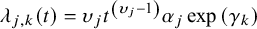 $$\begin{align}{\lambda}_{j,k}(t)={\upsilon}_j{t}^{\left({\upsilon}_j-1\right)}{\alpha}_j\exp \left({\gamma}_k\right)\end{align}$$
and the survivor function is
 $$\begin{align}{S}_{j,k}(t)=\exp \left(-{\alpha}_j\exp \left({\gamma}_k\right){t}^{\upsilon_j}\right),\end{align}$$
where ${\gamma}_1$
= 0, as treatment 1 is the “reference treatment.” As such, each study has a unique baseline hazard function (
${\gamma}_1$
= 0, as treatment 1 is the “reference treatment.” As such, each study has a unique baseline hazard function ( ${\lambda}_{j,1}(t)={\upsilon}_j{t}^{\upsilon_j-1}{\alpha}_j$
) defined by the shape parameter,
${\lambda}_{j,1}(t)={\upsilon}_j{t}^{\upsilon_j-1}{\alpha}_j$
) defined by the shape parameter, ${\upsilon}_j$
, and scale parameter,
${\upsilon}_j$
, and scale parameter, ${\alpha}_j$
, for study j, in 1,…,J. This specification restricts the scale and shape parameters to
${\alpha}_j$
, for study j, in 1,…,J. This specification restricts the scale and shape parameters to ${\alpha}_j$
> 0 and
${\alpha}_j$
> 0 and ${\upsilon}_j$
> 0, for j in 1,…,J, and for k in 1,…,K. It is noteworthy that when the shape parameter,
${\upsilon}_j$
> 0, for j in 1,…,J, and for k in 1,…,K. It is noteworthy that when the shape parameter, ${\upsilon}_j,$
is <1, the hazard rate decreases over time, whereas when
${\upsilon}_j,$
is <1, the hazard rate decreases over time, whereas when ${\upsilon}_j$
is >1, the hazard rate increases over time. When
${\upsilon}_j$
is >1, the hazard rate increases over time. When ${\upsilon}_j=1$
, the hazard rate is constant over time, and the Weibull reduces to the exponential distribution.
${\upsilon}_j=1$
, the hazard rate is constant over time, and the Weibull reduces to the exponential distribution.
The treatment effect is represented by ${\gamma}_k$
, and PhillippoReference Phillippo31 proposes that priors for the model parameters can be specified as
${\gamma}_k$
, and PhillippoReference Phillippo31 proposes that priors for the model parameters can be specified as
 $$\begin{align}\log \left({\unicode{x3b1}}_{\mathrm{j}}\right)\sim \mathrm{Normal}\big(0,{100}^2\big),\mathrm{for}\;{j}\;\mathrm{in}\;1,\dots, {J};\end{align}$$
 $$\begin{align}{\upsilon}_{\mathrm{j}}\sim \mathrm{Uniform}\left(0,+\infty \right),\mathrm{for}\;{j}\;\mathrm{in}\;1,\dots, {J};\mathrm{and}\end{align}$$
 $$\begin{align}{\unicode{x3b3}}_{\mathrm{k}}\sim \mathrm{Normal}\big(0,{100}^2\big),\mathrm{for}\;{k}\;\mathrm{in}\;2,\dots, {K}.\end{align}$$
We extend the PH Weibull model proposed by PhillippoReference Phillippo31 by defining the hazard function as:
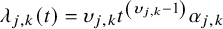 $$\begin{align}{\lambda}_{j,k}(t)={\upsilon}_{j,k}{t}^{\left({\upsilon}_{j,k}-1\right)}{\alpha}_{j,k}\end{align}$$
and the survivor function as
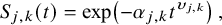 $$\begin{align}{S}_{j,k}(t)=\exp \!\left(-{\alpha}_{j,k}{t}^{\upsilon_{j,k}}\right),\end{align}$$
where ${\alpha}_{j,k}$
is the scale parameter and
${\alpha}_{j,k}$
is the scale parameter and ${\upsilon}_{j,k}$
is the shape parameter for the k-th treatment in the j-th study. An NMA model with an arm-based likelihoodReference Phillippo31 is then specified as
${\upsilon}_{j,k}$
is the shape parameter for the k-th treatment in the j-th study. An NMA model with an arm-based likelihoodReference Phillippo31 is then specified as
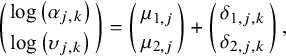 $$\begin{align}\left(\genfrac{}{}{0pt}{}{\log \left({\alpha}_{j,k}\right)}{\log \left({\upsilon}_{j,k}\right)}\right)=\left(\genfrac{}{}{0pt}{}{\mu_{1,j}}{\mu_{2,j}}\right)+\left(\genfrac{}{}{0pt}{}{\delta_{1,j,k}}{\delta_{2,j,k}}\right),\end{align}$$
where ${\delta}_{1,j,1}={\delta}_{2,j,1}=0$
, for j in 1,…,J. It is noteworthy that, in this notation, the first subscript used for
${\delta}_{1,j,1}={\delta}_{2,j,1}=0$
, for j in 1,…,J. It is noteworthy that, in this notation, the first subscript used for $\mu$
and
$\mu$
and $\delta$
differentiates between the shape and scale parameters. Also note that the PH Weibull model from Phillippo31 can be recovered by setting:
$\delta$
differentiates between the shape and scale parameters. Also note that the PH Weibull model from Phillippo31 can be recovered by setting: ${\delta}_{1,j,k}={\gamma}_k$
,
${\delta}_{1,j,k}={\gamma}_k$
, ${\mu}_{1,j}={\alpha}_j$
,
${\mu}_{1,j}={\alpha}_j$
, $\exp \left({\mu}_{2,j}\right)={\upsilon}_j$
, and
$\exp \left({\mu}_{2,j}\right)={\upsilon}_j$
, and $\exp \left({\delta}_{2,j,k}\right)=1.$
A fixed-effect (FE) NMA model sets ${\delta}_{1,j,k}$
=
${\delta}_{1,j,k}$
= ${d}_{1,k}$
and
${d}_{1,k}$
and ${\delta}_{2,j,k}$
=
${\delta}_{2,j,k}$
= ${d}_{2,k}$
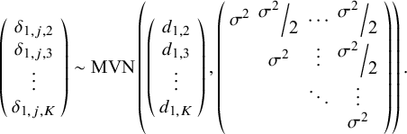
, for k in 1,…,K, so that treatment effects are not study-specific. Alternatively, a random-effects (RE) NMA model is specified with study-specific treatment effects such that, for j in 1,…,J, we define the following multivariate normal distribution:
${d}_{2,k}$
, for k in 1,…,K, so that treatment effects are not study-specific. Alternatively, a random-effects (RE) NMA model is specified with study-specific treatment effects such that, for j in 1,…,J, we define the following multivariate normal distribution:
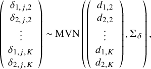 $$\begin{align}\left(\begin{array}{c}{\delta}_{1,j,2}\\ {}{\delta}_{2,j,2}\\ {}\begin{array}{c}\vdots \\ {}{\delta}_{1,j,K}\\ {}{\delta}_{2,j,K}\end{array}\end{array}\right)\sim \mathrm{MVN}\left(\left(\begin{array}{c}{d}_{1,2}\\ {}{d}_{2,2}\\ {}\begin{array}{c}\vdots \\ {}{d}_{1,K}\\ {}{d}_{2,K}\end{array}\end{array}\right),{\Sigma}_{\delta}\right),\end{align}$$
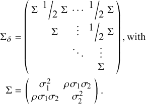
where ${\Sigma}_{\delta }$
, the 2(K−1) by 2(K−1) covariance matrix (following Cope et al.Reference Cope, Chan and Jansen22), is defined as
${\Sigma}_{\delta }$
, the 2(K−1) by 2(K−1) covariance matrix (following Cope et al.Reference Cope, Chan and Jansen22), is defined as
For both the FE and RE models, the ${d}_{1,k}$
and
${d}_{1,k}$
and ${d}_{2,k}$
parameters represent the relative effect of treatment k versus treatment 1 within each of the J study populations (see White et al.Reference White, Turner, Karahalios and Salanti32).
${d}_{2,k}$
parameters represent the relative effect of treatment k versus treatment 1 within each of the J study populations (see White et al.Reference White, Turner, Karahalios and Salanti32).
All Bayesian models require defining priors for all model parameters. For j in 1,…,J, and for k in 2,…,K, wide Normal priors with a mean of 0 and a variance of 1,000 can be specified for ${\mu}_{1,j}$
,
${\mu}_{1,j}$
, ${\mu}_{2,j}$
and for
${\mu}_{2,j}$
and for ${d}_{1,k}$
and
${d}_{1,k}$
and ${d}_{2,k}$
(also following Cope et al.Reference Cope, Chan and Jansen22):
${d}_{2,k}$
(also following Cope et al.Reference Cope, Chan and Jansen22):
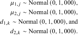 $$\begin{align*}{\mu}_{1,j}\sim \mathrm{Normal}\left(0,\mathrm{1,000}\right)\!,\\{\mu}_{2,j}\sim \mathrm{Normal}\left(0,\mathrm{1,000}\right)\!,\\{d}_{1,k}\sim \mathrm{Normal}\left(0,\mathrm{1,000}\right)\!,\mathrm{and}\\{d}_{2,k}\sim \mathrm{Normal}\left(0,\mathrm{1,000}\right)\!.\end{align*}$$
In the RE NMA, a prior is also needed for $\Sigma$
(or alternatively for the individual
$\Sigma$
(or alternatively for the individual ${\sigma}_1$
,
${\sigma}_1$
, ${\sigma}_2$
, and
${\sigma}_2$
, and $\rho$
parameters). Following Cope et al.Reference Cope, Chan and Jansen22 and Jansen Reference Jansen19 we can define the following Inverse-Wishart prior:
$\rho$
parameters). Following Cope et al.Reference Cope, Chan and Jansen22 and Jansen Reference Jansen19 we can define the following Inverse-Wishart prior:
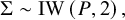 $$\begin{align*}\Sigma \sim \mathrm{IW}\left(P,2\right),\end{align*}$$
where P is a given 2 by 2 scale matrix.
It is noteworthy that, alternatively, a somewhat less complex RE model could be defined whereby RE are specified for only one of the two treatment effect parameters. This simpler model could be useful when there are reasons to believe that one parameter varies between studies while the rest remain relatively constant. For example, a model could define study-specific treatment effects with respect to the scale parameter, while the shape parameter would remain fixed across studies. For instance, one could define, for k in 1, …,K, ${\delta}_{2,j,k}$
=
${\delta}_{2,j,k}$
= ${d}_{2,k}$
, and for j in 1,…, J:
${d}_{2,k}$
, and for j in 1,…, J:
We also note that alternative prior specifications are also possible, and various parameterizations of the variance–covariance matrix specified in equations (11) and (12) could be considered (see Wei and HigginsReference Wei and Higgins33). Our multivariate Weibull NMA model can be easily generalized to other parametric distributions. We outline standard parametric models in Table 1, including the Weibull, Gompertz, log-normal, log-logistic, gamma, and generalized gamma distributions. The generalized gamma distribution is characterized by three parameters and in our NMA model; only two of these three parameters are study- and treatment-specific. The third parameter, Q, is assumed to have the same value for all individuals across all studies and treatments within the network.
Table 1 Survival and hazard functions for standard parametric survival models
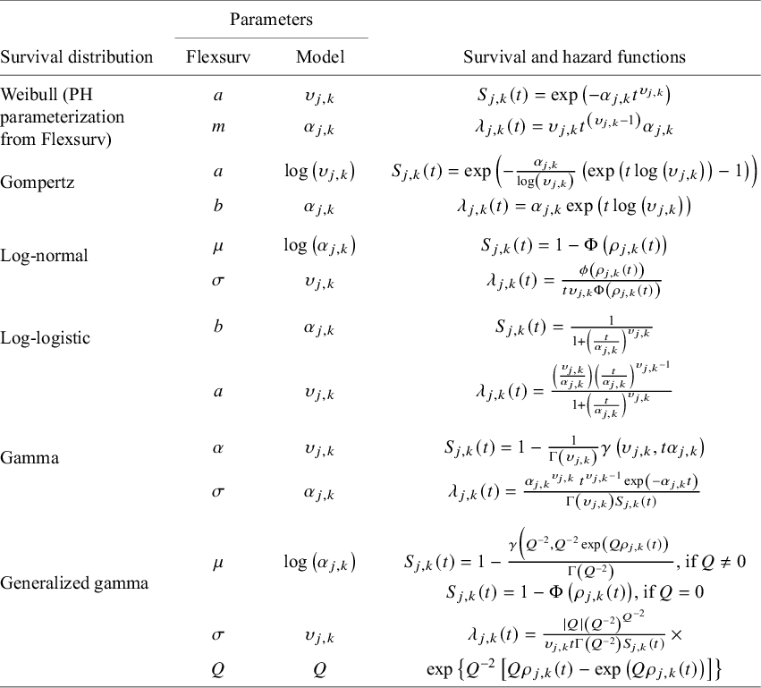
Note: For reference, the parameterization used (“standard parameterization”) corresponds to that used in the flexsurv R packageReference Jackson23 following the equivalences listed in the “Parameters” columns. Recall that our model specification (equation (9)) restricts the scale and shape parameter to be strictly positive (i.e., ${\alpha}_{j,k}$
> 0 and
${\alpha}_{j,k}$
> 0 and ${\upsilon}_{j,k}$
> 0, for j in 1,…,J, and for k in 1,…,K). Note that
${\upsilon}_{j,k}$
> 0, for j in 1,…,J, and for k in 1,…,K). Note that $\phi \left(\bullet \right)$
and
$\phi \left(\bullet \right)$
and $\varPhi \left(\bullet \right)$
denote the probability density function and the cumulative density function of the standard normal distribution, respectively;
$\varPhi \left(\bullet \right)$
denote the probability density function and the cumulative density function of the standard normal distribution, respectively; $\varGamma \left(\bullet \right)$
and
$\varGamma \left(\bullet \right)$
and $\gamma \left(\bullet, \bullet \right)$
denote the gamma function and the incomplete gamma function, respectively; and
$\gamma \left(\bullet, \bullet \right)$
denote the gamma function and the incomplete gamma function, respectively; and ${\rho}_{j,k}(t)=\left[\mathit{\log}(t)-\mathit{\log}\left({\alpha}_{j,k}\right)\right]/{\upsilon}_{j,k}$
.
${\rho}_{j,k}(t)=\left[\mathit{\log}(t)-\mathit{\log}\left({\alpha}_{j,k}\right)\right]/{\upsilon}_{j,k}$
.
3 Simulation study
In this section, we consider a simple simulation study to investigate the validity of the proposed one-step model and compare it to the two-step model. In this simulation study, both the proposed one-step model and two-step model from Cope et al.Reference Cope, Chan and Jansen22 are used to analyze 5,000 simulated datasets, assuming FE with the Weibull distribution. Jackson and WhiteReference Jackson and White29 suggest that a one-step approach may be preferable due to the “hidden normality” assumptions required with a two-step approach, which can, at least in theory, “have serious implications for the accuracy of the resulting statistical inference.” The simulation study is based on the work in Section 7.3 of Phillippo,Reference Phillippo31 where a single simulated dataset is considered consisting of two RCTs: one trial comparing treatments A versus B, and the other trial comparing treatments A versus C. Here, we extend the network to include a third trial comparing treatments C versus D. In the Supplementary Material, additional analyses are presented to demonstrate how the proposed one-step model fits when different distributions are assumed.
3.1 Data-generating mechanism
As illustrated in Figure 1, each artificial dataset includes survival data for three two-arm RCTs: Study j = 1 compares treatment k = 2 to k = 1 (henceforth, “Study AB” comparing intervention B with A); Study j = 2 compares treatment k = 3 to k = 1 (“Study AC”); and Study j = 3 compares treatment k = 4 to k = 3 (“Study CD”). Each study consists of Nstudy individuals randomly assigned (with a 1:1 randomization ratio) to one of the two treatment arms. We considered two scenarios: (1) with Nstudy = 36 and (2) with Nstudy = 100.
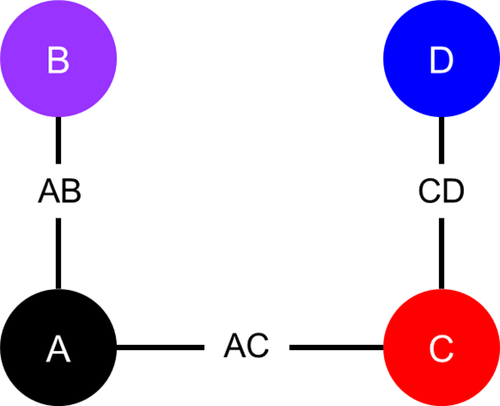
Figure 1 Network diagram of artificial randomized controlled trials.
We simulated survival times to obtain time-varying treatment effects. Specifically, survival times were simulated from Weibull distributions corresponding to the FE Weibull model outlined in equations (7)–(9) using the cumulative distribution function inversion method (as implemented in the R package simsurvReference Brilleman, Wolfe, Moreno-Betancur and Crowther34) with the following parameters: ${\mu}_{1,1}={\mu}_{1,2}={\mu}_{1,3}=1.5$
,
${\mu}_{1,1}={\mu}_{1,2}={\mu}_{1,3}=1.5$
, ${\mu}_{2,1}={\mu}_{2,2}={\mu}_{2,3}=0.5, {d}_{1,2}=1.2$
,
${\mu}_{2,1}={\mu}_{2,2}={\mu}_{2,3}=0.5, {d}_{1,2}=1.2$
, ${d}_{2,2}=0.6,{d}_{1,3}=0.5,$ ${d}_{2,3}=-0.3,{d}_{1,4}=-0.5,$
and
${d}_{2,3}=-0.3,{d}_{1,4}=-0.5,$
and ${d}_{2,4}=-0.7$
.
${d}_{2,4}=-0.7$
.
Potential censoring times were simulated independently of event times from a Uniform(0,1) distribution, and a random 10% of individuals were selected for potential censoring. An individual was ultimately censored if their survival time was greater than their potential censoring time. All individuals who had not experienced an event by 1 year were censored at 1 year. KM plots illustrate the event and censor times for one of the simulated datasets in Figure 2.
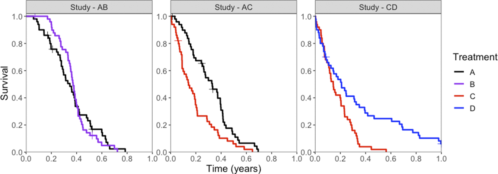
Figure 2 Kaplan–Meier survival curves for simulated event times, for each treatment (colors) in each study (panels). Censored events are marked with a cross (“+”).
3.2 Methods to estimate treatment effects based on the simulated data
The relative treatment effects for the competing interventions based on the artificial RCTs in the network were assessed using a one-step FE IPD-NMA model assuming a Weibull distribution for event times (as outlined in equations (7)–(9)). For comparison, we also fit the data using the two-step approach of Cope et al.,Reference Cope, Chan and Jansen22 also assuming an FE model and a Weibull distribution. Both the one-step and two-step models used the parameterization specified in Table 1. The parameters for these models were estimated using the Markov Chain Monte Carlo (MCMC) method using R (packages: rstan, loo, and flexsurvReference Jackson23) and Stan,Reference Phillippo35– 37 where an initial series of 2,000 iterations from the sampler was discarded (i.e., burn-in) and inferences were based on subsequent 2,000 iterations using four chains.
Results for each dataset were summarized in terms of the posterior medians and 95% credible intervals (CrIs). For each of the two Nstudy scenarios, across all 5,000 datasets, the mean bias, mean credible interval coverage, and mean credible interval width were calculated.
3.3 Results
Results are summarized in Table 2 and suggest that the NMA estimates obtained from both the one-step and two-step models have little to no bias and that both methods provide 95% CrIs with approximately correct coverage (i.e., the 95% CrIs obtained contain the true parameter value ~95% of the time). For almost all parameter estimates, the one-step method appears to be less biased than the two-step method. The average widths of the 95% CrIs are very similar for the one-step and two-step models, suggesting that both approaches are equally efficient. Comparing results from the Nstudy = 36 scenario with those from the Nstudy = 100 scenario, we see that with smaller sample sizes (i.e., with Nstudy = 36), the estimates have larger biases, and the 95% CrIs are perhaps slightly too narrow. Finally, with respect to the computational resources required, the one-step model took about twice as long to fit compared to the two-step model when Nstudy = 36 and about three times as long to fit when Nstudy = 100.
Table 2 Results from the simulation study: for each parameter, the average estimate (averaged over the 2,000 simulated datasets); the bias (average estimate—truth); 95% CrI coverage (proportion of simulation for which the 95% CrI contained the true parameter value); and average 95% CrI width (averaged over the 5,000 simulated datasets)
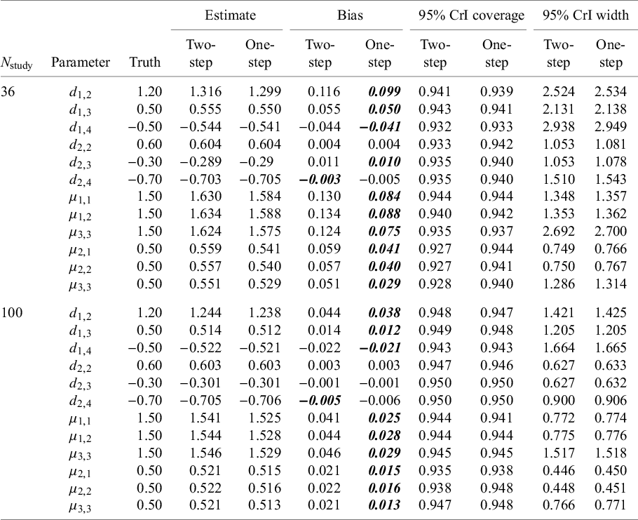
Note: Survival times were simulated from Weibull distributions corresponding to the FE Weibull model with the following parameters: ${\mu}_{1,1}={\mu}_{1,2}={\mu}_{1,3}=1.5$
,
${\mu}_{1,1}={\mu}_{1,2}={\mu}_{1,3}=1.5$
, ${\mu}_{2,1}={\mu}_{2,2}={\mu}_{2,3}=0.5,{d}_{1,2}=1.2$
,
${\mu}_{2,1}={\mu}_{2,2}={\mu}_{2,3}=0.5,{d}_{1,2}=1.2$
, ${d}_{2,2}=0.6,{d}_{1,3}=0.5,$ ${d}_{2,3}=-0.3,{d}_{1,4}=-0.5, \mathrm{and}\; {d}_{2,4}=-0.7$
. Bolded values indicate smaller bias value (comparing two-step vs. one-step).
${d}_{2,3}=-0.3,{d}_{1,4}=-0.5, \mathrm{and}\; {d}_{2,4}=-0.7$
. Bolded values indicate smaller bias value (comparing two-step vs. one-step).
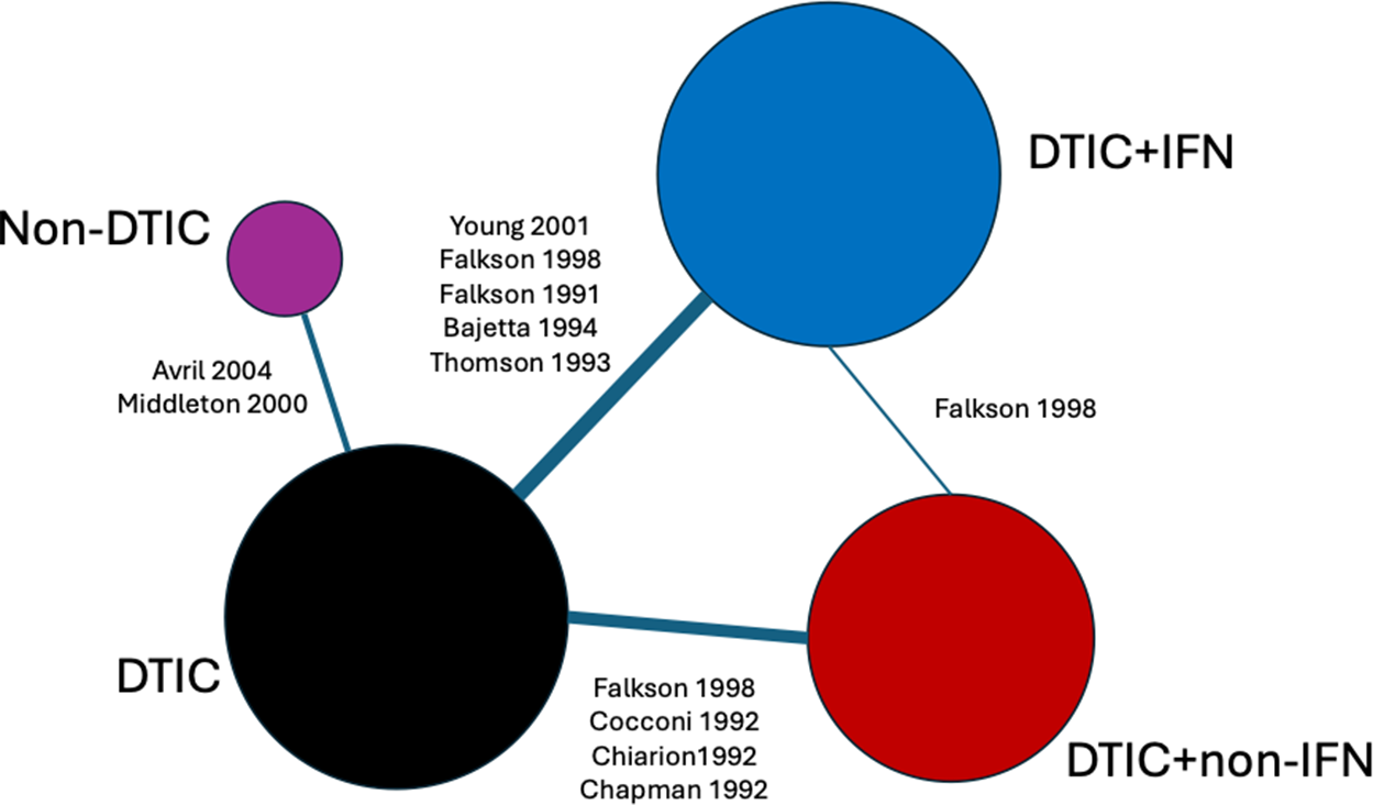
Figure 3 Network of evidence for melanoma randomized controlled trials. Node size and line thickness correspond to the number of studies, including the treatment and the treatment comparison. Abbreviations: DTIC, dacarbazine; IFN, interferon (IFN).
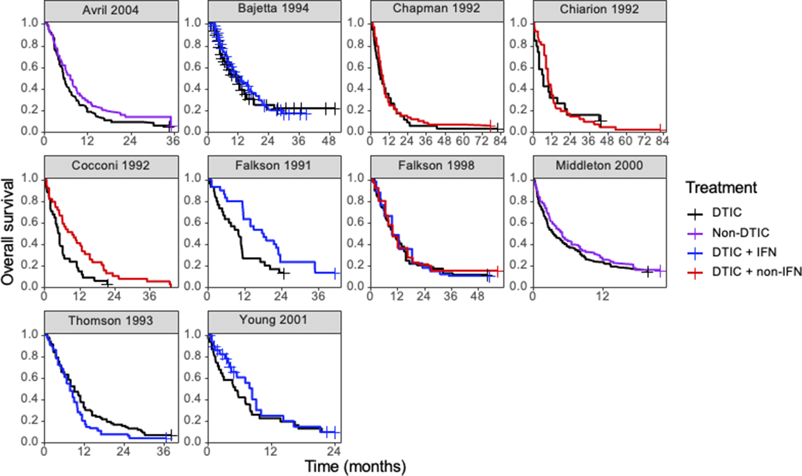
Figure 4 Kaplan–Meier plots of the reconstructed individual event and censoring times obtained for each randomized controlled trial. Abbreviations: DTIC, dacarbazine; IFN, interferon (IFN).
4 Illustrative examples with existing empirical data
The illustrative example was based on a network of studies concerning the treatment of advanced (Stage IIIc or IV) melanoma. Details of the network have been presented previously in Jansen et al. Reference Jansen, Vieira and Cope38 and Cope et al.Reference Cope, Chan and Jansen22 Notably, these studies are somewhat dated, having been published between 1991 and 2004, and we refer readers to Boutros et al.Reference Boutros, Croce and Ferrari39 for a review of the current treatment landscape.
Ten RCTs identified in a systematic literature review formed a connected network, illustrated in Figure 3, evaluating four treatments: dacarbazine (DTIC) monotherapy, DTIC + Interferon (IFN), DTIC + Non-IFN, and Non-DTIC. For each treatment arm in each RCT, the reported KM curves were digitized (DigitizeIt; http://www.digitizeit.de/), and the reconstructed individual event and censoring times were obtained using the Guyot et al.Reference Guyot, Ades, Ouwens and Welton20 algorithm (which was recently recommended by Saluja et al.Reference Saluja, Cheng, delos Santos and Chan40 following an assessment of its reliability, accuracy, and precision) (see Figure 4).
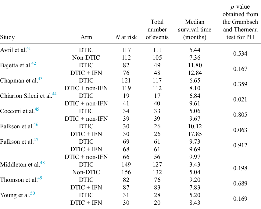
For each of the 10 studies in the melanoma network, Table 3 lists the number of patients per arm, the number of OS events per arm, the median survival time per arm, and the p-value obtained from applying the Grambsch and Therneau test for PH.Reference Grambsch and Therneau51 Notably, there is evidence of non-PH in the Chiarion 1992 study, which compared DTIC and DTIC + non-IFN (p-value = 0.021), and therefore, according to Cope et al.Reference Cope, Chan and Campbell14 and recent guidance (e.g., “if the PH assumption is deemed to be implausible for one or more comparisons in the network, then (network) meta-analysis of HRs should not be carried out”52), a method that does not require the PH assumption should be used for analysis.
Table 3 For each of the 10 studies in the melanoma network: the number of patients per arm, the number of overall survival events per arm, the median survival time per arm, and the p-value obtained from applying the Grambsch and Therneau test for proportional hazard (PH) assumption
4.1 Methods
We fit the one-step and two-step multivariate NMA models with both the fixed and the REs using MCMC with R and StanReference Phillippo35–
37 as described in Section 3. We defined REs on both the shape and scale parameters (following equation (10)) and specified an Inverse-Wishart prior for $\Sigma$
(following equation (11)) with:
$\Sigma$
(following equation (11)) with:
 $$\begin{align*}P=\left(\begin{array}{cc}1/10& 0\\ {}0& 1/10\end{array}\right).\end{align*}$$
Consistent with Cope et al.,Reference Cope, Chan and Jansen22 we considered four different distributions for the likelihood: the Weibull, the Gompertz, the log-normal, and log-logistic. It is noteworthy that, for the two-step approach, the parameterization originally used by Cope et al.Reference Cope, Chan and Jansen22 was based on models originally proposed by Ouwens et al.Reference Ouwens, Philips and Jansen18 In contrast, we fit all models with the more familiar parameterization detailed in Table 1.
The approximate leave-one-out (LOO) information criterion (LOOIC) was used to select the most appropriate model. The LOOIC is similar to the DIC in that smaller values signal better model fit, but, unlike the DIC, it is invariant to parametrization and corresponds to a model’s predictive performance (integrating over the posterior distribution of the parameters) (see Vehtari et al.Reference Vehtari, Gelman and Gabry53). Convergence for each parameter was assessed using the Gelman-Rubin statistic.Reference Gelman and Rubin54, Reference Gelman55 Checks for divergent transitions were also performed (see Betancourt et al.Reference Betancourt and Girolami56).
4.2 Results
All models converged and appeared to fit the data reasonably well (see predicted survival curves in Figures 5 and 6, and MCMC trace plots for the log-logistic models in Figures 7 and 8). However, for all models to successfully converge, the RStan default settings for the “adapt_delta” and “max_treedepth” control variables needed to be changed following current recommendations (see details in code provided in the Supplemental Materials).37 On a laptop computer (Macbook Pro, with M1 chip and 16 GB memory), the two-step models all took less than a minute to fit, whereas the one-step models took between 1 and 188 minutes (with RE models taking about two and a half times longer to fit than FE models; see Table 4).
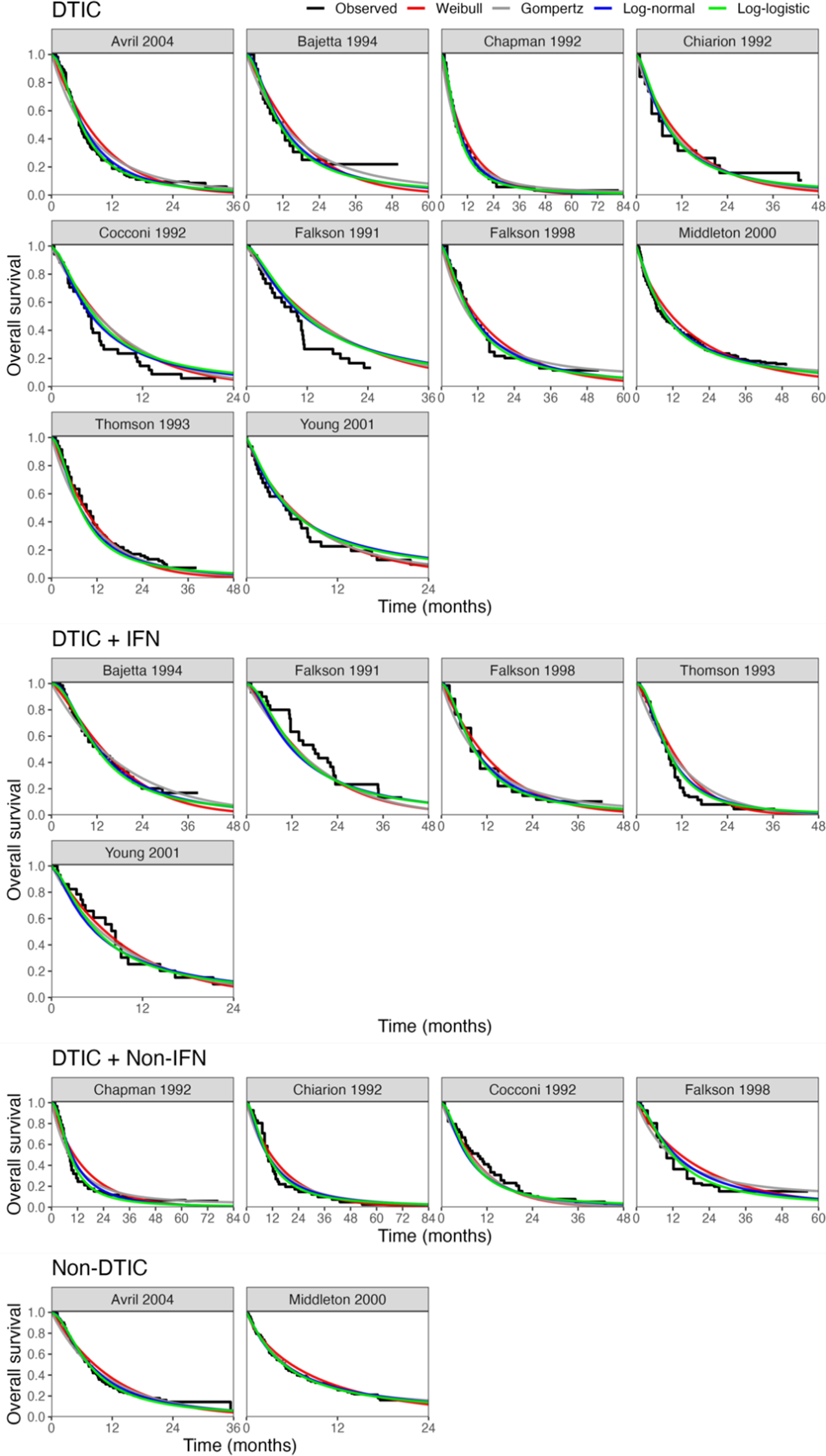
Figure 5 Fitted survival functions for all distributions from FE one-step model (Weibull, Gompertz, log-normal, and log-logistic) and Kaplan–Meier curves by treatment arm. Abbreviations: DTIC, dacarbazine; IFN, interferon (IFN).
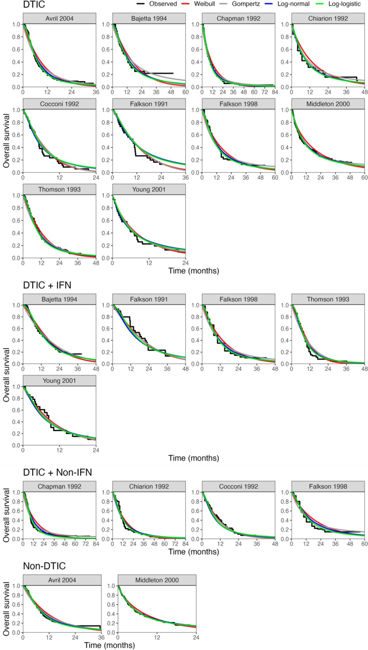
Figure 6
Fitted study-specific survival functions (using study-specific baseline risk [ ${\boldsymbol{\mu}}_{\boldsymbol{1},\boldsymbol{j}}\;\boldsymbol{and}\;{\boldsymbol{\mu}}_{\boldsymbol{1},\boldsymbol{j}}$
] and relative treatment effects [
${\boldsymbol{\mu}}_{\boldsymbol{1},\boldsymbol{j}}\;\boldsymbol{and}\;{\boldsymbol{\mu}}_{\boldsymbol{1},\boldsymbol{j}}$
] and relative treatment effects [ ${\boldsymbol{\delta}}_{\boldsymbol{1},\boldsymbol{j},\boldsymbol{k}}\;\boldsymbol{and}\;{\boldsymbol{\delta}}_{\boldsymbol{2},\boldsymbol{j},\boldsymbol{k}}$
]) for all distributions from the RE one-step model (Weibull, Gompertz, log-normal, and log-logistic) and Kaplan–Meier curves by treatment arm. Abbreviations: DTIC, dacarbazine; IFN, interferon (IFN).
${\boldsymbol{\delta}}_{\boldsymbol{1},\boldsymbol{j},\boldsymbol{k}}\;\boldsymbol{and}\;{\boldsymbol{\delta}}_{\boldsymbol{2},\boldsymbol{j},\boldsymbol{k}}$
]) for all distributions from the RE one-step model (Weibull, Gompertz, log-normal, and log-logistic) and Kaplan–Meier curves by treatment arm. Abbreviations: DTIC, dacarbazine; IFN, interferon (IFN).
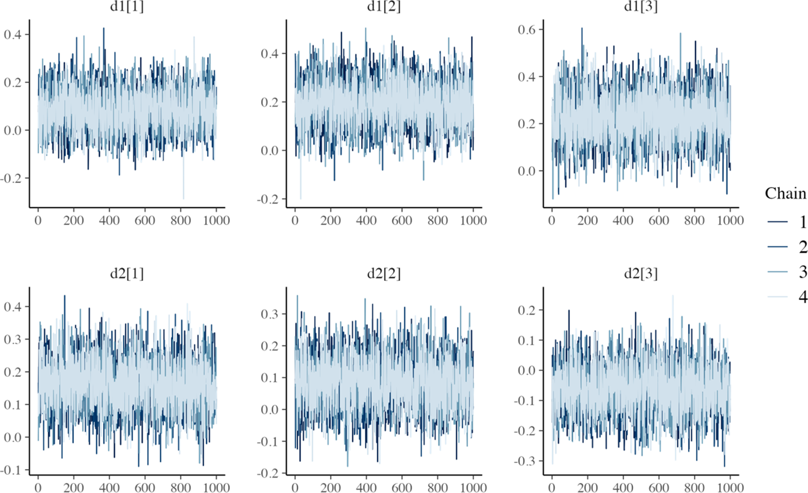
Figure 7 MCMC trace plots for relative treatment effect parameters of the one-step FE log-logistic NMA model.
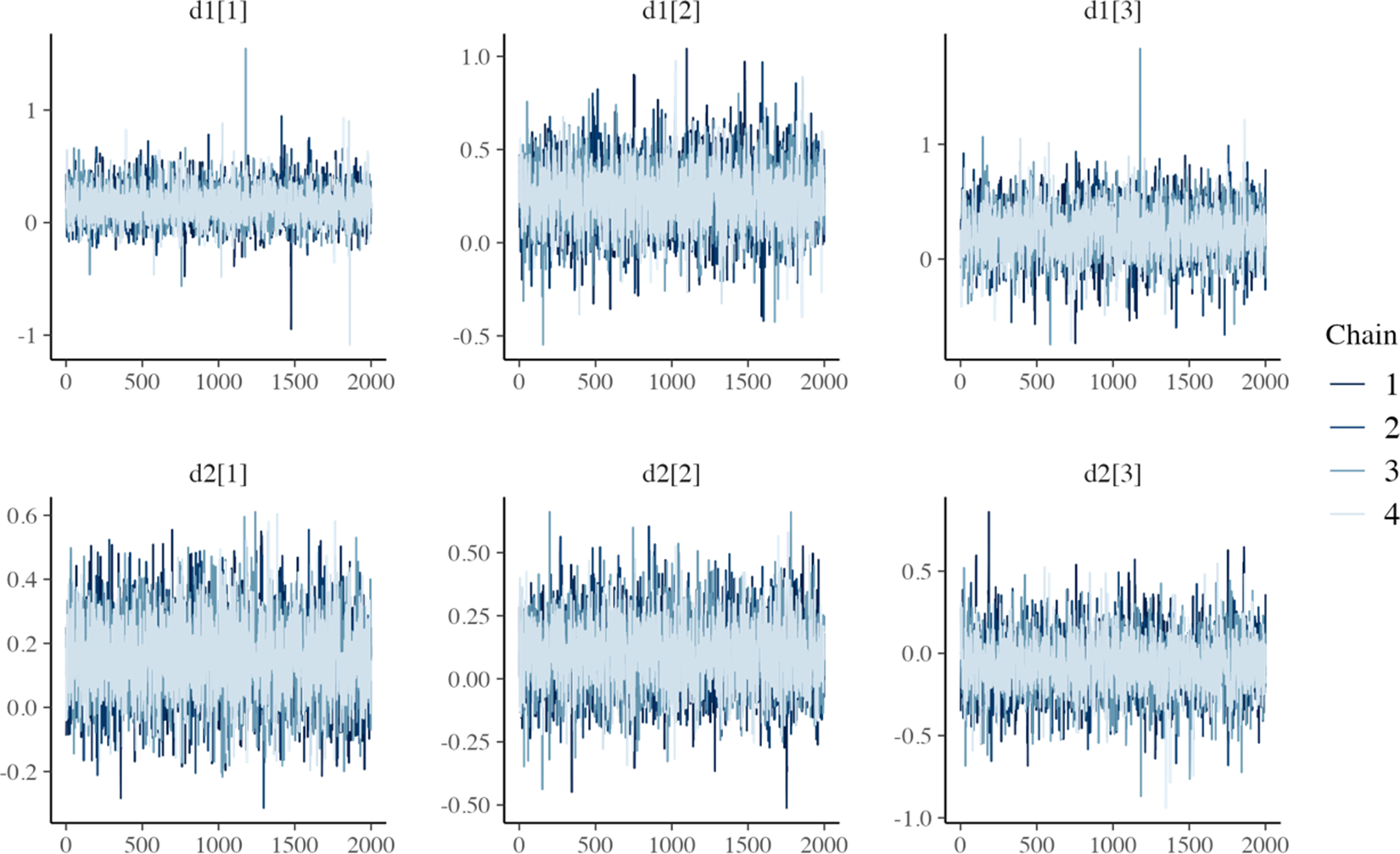
Figure 8 MCMC trace plots for relative treatment effect parameters of the one-step RE log-logistic NMA model.
The LOOIC suggests that the log-logistic distribution was most appropriate (Table 4), which is consistent with findings by Cope et al.Reference Cope, Chan and Jansen22 based on the sum of treatment-arm specific AIC values per distribution in the first step of their analysis. The parameter estimates and 95% CrIs for the one-step log-logistic random-effects (and fixed-effect) model are very similar to those obtained using the two-step NMA method (Table 5). The small discrepancies between the estimates may be explained by the assumptions required in the two-step NMA regarding within-study estimates in terms of normality and standard errors and/or by the different priors required for the one-step and two-step models. These findings were consistent across the alternative distributions for the likelihood evaluated (Table 6), which are summarized in terms of the predicted survivals in Figures 5 and 6.
Figure 9 plots the estimated survival curves from the FE and RE one-step models fit to a population with the same baseline risk as the Avril 2004 study population. Within the first 6 months, survival appears highest for DTIC + non-IFN. However, the DTIC + non-IFN and non-DTIC survival curves cross shortly after 6 months (illustrating the effect of time-varying treatment effects), and among all four treatments, long-term survival appears highest for non-DTIC.
Table 4 Computational sampling time required for each model and leave-one-out information criterion (LOOIC)
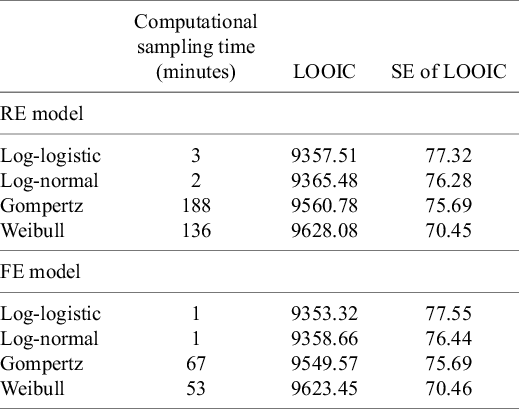
Note: The LOOIC can be used to select the most appropriate model. The distribution with the lowest LOOIC values, the log-logistic in this case (for both random effects [REs] and fixed effect [FE]), is considered the “best” model. Abbreviation: SE, standard error.
Table 5 Parameter estimates (posterior medians and 95% CrIs) obtained with random-effects (REs) and fixed-effect (FE) log-logistic NMA models: (1) two-step multivariate network meta-analysis model (Cope et al.Reference Cope, Chan and Jansen22) versus (2) the proposed one-step IPD NMA
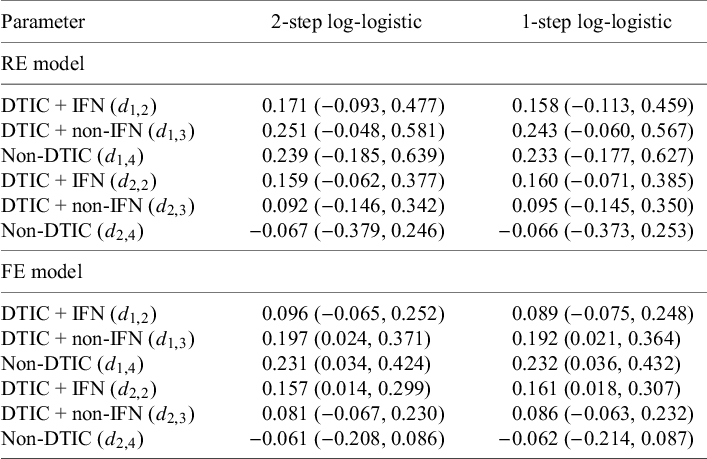
Table 6 Parameter estimates (posterior medians and 95% CrIs) obtained with random-effects (REs) and fixed-effect (FE) NMA models: (1) two-step multivariate network meta-analysis model (Cope et al.Reference Cope, Chan and Jansen22) versus (2) the proposed one-step IPD NMA
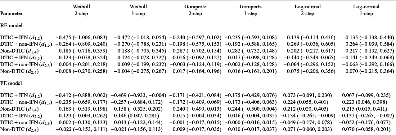
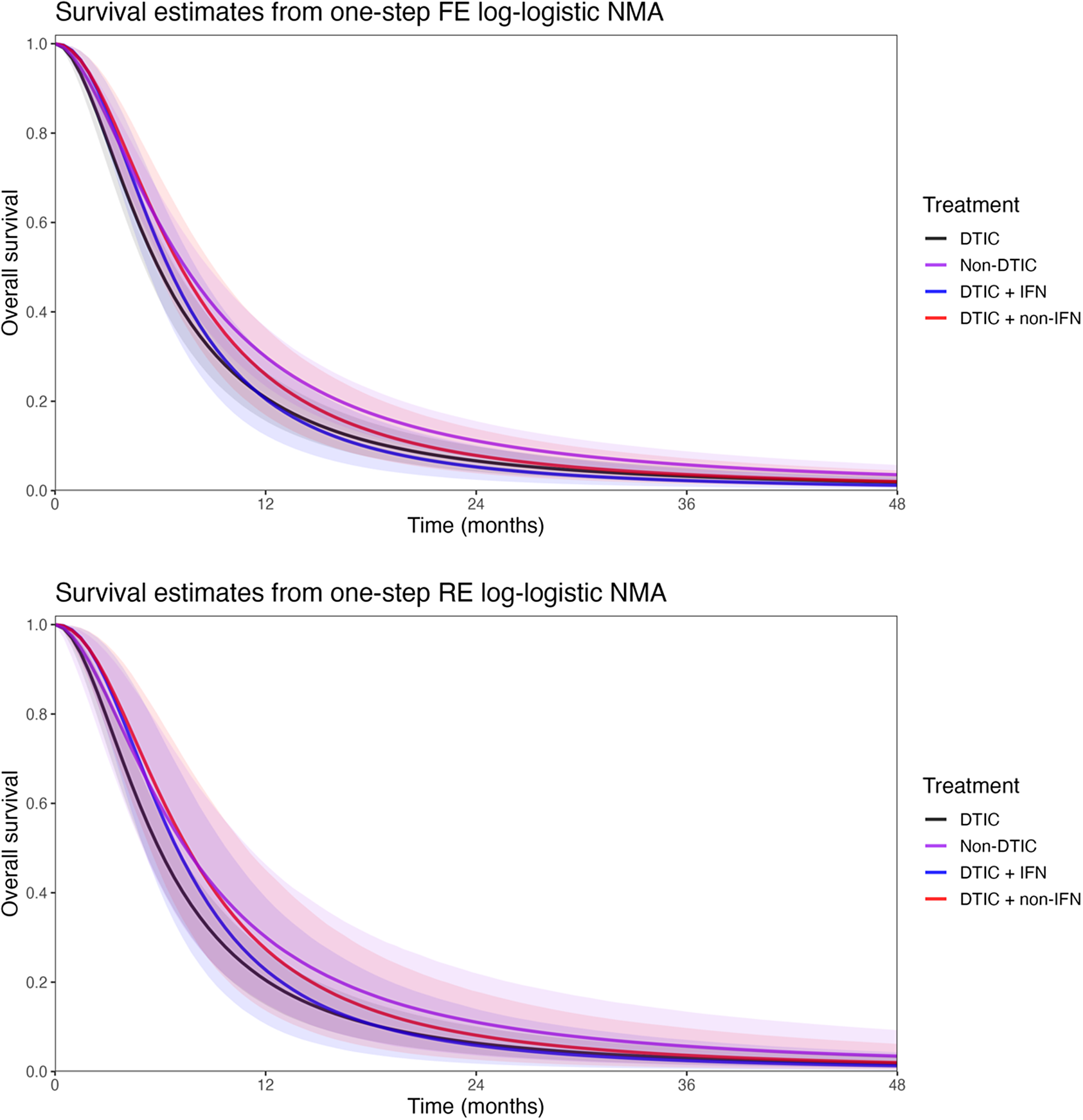
Figure 9 Posterior estimates of overall survival (with shaded 95% CrIs) comparing DTIC, DTIC + IFN, DTIC + non-IFN, and Non-DTIC in the Avril 2004 population from the one-step NMA FE (top panel) and RE (bottom panel) models. Abbreviations: DTIC, dacarbazine; IFN, interferon (IFN).
Table 7 Estimates obtained from the one-step and two-step log-logistic models regarding overall survival at 1 year and at 2 years comparing DTIC + IFN and non-DTIC fit for a population with baseline risk of the Avril 2004 study population
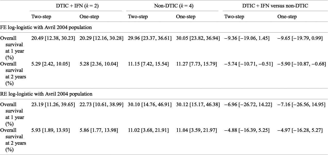
The treatment effect estimates can be summarized in many ways, and Cope and JansenReference Cope and Jansen57 consider how various quantitative summaries compare using the same melanoma network as an illustrative example.Reference Cope and Jansen57 Suppose one was specifically interested in OS at 1 year and at 2 years, and was interested in comparing DTIC + IFN and non-DTIC, a treatment comparison for which there is no direct evidence. Table 7 lists the relevant estimates obtained from the one-step and two-step log-logistic models fit to a population with the same baseline risk as the Avril 2004 study population. Briefly, with the one-step FE log-logistic model, the OS at 1 year with DTIC + IFN is estimated to be 20% (95% CrI: [12%, 30%]), slightly lower than with non-DTIC: 30% (95% CrI: [24%, 37%]). The estimated difference in OS at 1 year is −10% (95% CrI: [−20%, 1%]), and at 2 years is −6% (95% CrI: [−11%, −1%]). These findings were consistent for one-step and two-step models. Credible intervals are notably wider with RE models relative to FE models.
5 Discussion
The proposed multivariate NMA models for TTE outcomes provide a one-step framework that allows for time-varying treatment effects, which leverage exact (or reconstructed) event and censor times for the studies in a connected network of evidence. By using the exact likelihood specification, we avoid the assumptions regarding within-study normality and variance required in the two-step method (Cope et al.Reference Cope, Chan and Jansen22). This allows the entire model to be fit within a Bayesian framework, facilitating straightforward model selection and interpretation. Potential concerns regarding computational burden are mitigated by using Stan software, which provides a more efficient MCMC sampling than previous software (i.e., WinBUGS or JAGS) through the implementation of the Hamiltonian Monte Carlo algorithm (see Monnahan et al.Reference Monnahan, Thorson and Branch58).
While we discussed using the LOOIC for model selection, often, valuable insight regarding the plausibility of different models may also be obtained from clinical expertsReference Latimer59– Reference Latimer61 and observational studies.Reference Ruiz-Morales, Swierkowski and Wells62 Moreover, when there is no reason to believe that treatment effects vary over time, simpler models with fewer parameters may be more appropriate. Cope et al.Reference Cope, Chan and Campbell14 previously proposed a stepwise process exploring standard parametric models with treatment effect on scale alone, followed by models with multivariate treatment effects (scale and shape) for each trial and network (or other more flexible models), which builds upon the process outlined by Latimer et al.Reference Latimer59 for survival analysis of a single RCT in context of cost-effectiveness analysis. The proposed one-step models allow this process to be applied to all the “standard” distributions, now including gamma and generalized gamma. Further, the generalized gamma distribution may be particularly useful to improve fit over other standard distributions to a network of RCTs given the flexibility to model U-shaped hazards with this distributionReference Cox, Chu, Schneider and Munoz63 as well as the nature of its nested distributions (i.e., exponential, Weibull, log-normal, and gamma).
The simulation study in Section 3 found that the proposed one-step method and the previously proposed two-step method provide broadly similar results. When study sample sizes are especially small, the one-step method may be preferred, in line with previous recommendations.Reference Jackson and White29 However, due to finite computational resources, the simulation study was limited in that we were unable to consider fitting RE models and did not consider a wide range of sample sizes and prior specifications. More extensive simulation studies may be helpful to better understand the impact of model misspecification, the differences between fitting FE and RE models, and the differences between using one-step and two-step methods.Reference Heinze, Boulesteix, Kammer, Morris and White64
The illustrative melanoma example highlighted an application to a network of multiple trials, where we demonstrated the feasibility of accounting for between-study heterogeneity in terms of both the shape and the scale parameters. However, simpler random-effect models specified for only one of the two treatment effect parameters may often be sufficient. We advise consulting clinicians to consider whether between-study heterogeneity is most likely to affect the scale versus the shape of the distributions. Future research should consider the merits of using different priors and parameterizations for the variance–covariance matrix,Reference Wang, Lin, Hodges and Chu65, Reference Alvarez, Niemi and Simpson66 potentially based on incorporating external evidence on the between-trial heterogeneity.Reference Turner, Domínguez-Islas, Jackson, Rhodes and White67
It may be of interest to extend the proposed methods to nonparametric IPD-NMA models. While potentially flexible, nonparametric models can be considerably more complex and may not be among the first NMA models to consider when following recommended model selection procedures in the broader cost-effectiveness framework.Reference Latimer59 Nonetheless, there may be utility in extending the current framework to include additional nonparametric methods.
During the development of this publication, Phillippo et al. proposed the extension the ML-NMR framework for TTE data, considering networks in which IPD-level covariate data is only available for a subset of trials within the network (with aggregate-level covariate data available for the remaining studies).Reference Phillippo, Dias, Ades and Welton68 This allows for the adjustment of prognostic factors and effect modifiers when information on these is available. Maciel et al.Reference Maciel, Cope and Towle69 demonstrated the feasibility of applying ML-NMR for TTE outcomes with a univariate treatment effect. The main advantage of NMA models with a multivariate treatment effect as proposed is that they do not rely on a PH assumption across studies and treatment comparisons. This flexibility may be important when there are differences in the survival distributions for the treatments compared, and relative treatment effects need to be extrapolated beyond the available trial data for a cost-effectiveness analysis.
Author contributions
Concept and design: H.C., D.M., K.C., J.J., S.K., K.T., B.M., and S.C.; Statistical analysis: D.M. and H.C.; Analysis and interpretation of results: H.C., D.M., K.C., J.J., S.K., K.T., B.M., and S.C.; Drafting of the manuscript: H.C. and S.C.; Critical revision of the paper for important intellectual content: H.C., D.M., K.C., J.J., S.K., K.T., B.M., and S.C.; Obtaining funding: S.K. and S.C.; Administrative, technical, or logistic support: K.T.; Supervision: S.C.
Competing interest statement
S.K. and B.M. are employees of Bristol Myers Squibb. H.C., D.M., K.C., J.J., K.T., and S.C. are employees of Precision AQ, a consulting firm that received funding from Bristol Myers Squibb for this study.
Data availability statement
We provide Stan code for both the two-step and one-step FE and RE models in the Supplementary Material. Also in the Supplementary Material, R code and data are provided to fit the one-step NMA models to the illustrative melanoma example from Section 4.
Funding statement
Funding for this study was provided by Bristol Myers Squibb.
Supplementary material
To view supplementary material for this article, please visit http://doi.org/10.1017/rsm.2025.21.


 Open access