The single greatest hurdle to the advancement of the scientific understanding of our own species is the difficulty in drawing causal inferences from the methods of study allowed by practical and ethical constraints. Even when such considerations allow one to perform experiments, the informativeness of such studies is often severely constrained by the gap between experimental and real-world conditions. Analyzing real-world data hardly improves the situation, as the use of natural experiments to justify causal inferences typically only advances our understanding so far, not least because of the comparative infrequency of natural experiments occurring in ideal form and being accompanied by effective measurement of the variables of interest.
However, one particular natural experiment was claimed to allow a unique degree of power and flexibility to address causal questions in the study of humans, at least when paired with a particular statistical procedure that could make the most use out of the information provided. The natural experiment in question was the production of twin births of two distinct types (mono and dizygotic), and the method was the direction of causation model. Before reviewing the model in greater detail below, it is worth considering what it aimed to deliver: For any two phenotypic characteristics, the method sought to explain the causal relationship between them, conditional on the characteristics having at least somewhat different modes of inheritance and there being sufficient numbers of twins assessed for the characteristics in question. The self-declared limitations of the method, then, are almost exclusively those pertaining to enrolling participants with an easily identifiable and not particularly rare characteristic (twin births typically occurring in at least 1% of most populations) and assessing them for whatever characteristics are of interest.
However, there has thus far been little critical discussion of the DoC model, and its adoption has been curiously piecemeal. For example, results from the model substantially affect the discussion in one area of our own research interest (concerning personality and politics), whereas researchers of many other topics have yet to be introduced to the method or results deriving from it, despite its apparent relevance and promised utility.
In the present work, we argue against further adoption of the DoC model by highlighting the consequences of one particular limiting assumption of the model that had not previously been closely discussed. This assumption is that of the absence of ‘non-shared confounding.’ Confounding is, of course, always a serious concern for observational research, but as we show, violations of this assumption are particularly devastating for the DoC model. In particular, we show that in a situation where features of the non-shared environment cause two traits to covary even to a relatively small degree, the DoC model dramatically misestimates both the size and direction of causal effects. An illustrative example of such non-shared confounding is provided by Sandewall et al. (Reference Sandewall, Cesarini and Johannesson2014), who found that among identical twins, within-pair differences in intelligence confounded the effect of education on earnings. Here, even though MZ twins are genetically identical and share their upbringing (and, as a result, share most confounders), non-shared confounding can still impair the ability to use twins to draw causal inferences. As we show below, such confounding would have posed a serious problem had the DoC model been applied to attempt to disentangle the causal relationship between education and earnings.
In this way, we show that the set of assumptions underlying the DoC model are even more restrictive than previously held (Heath et al., Reference Heath, Kessler, Neale, Hewitt, Eaves and Kendler1993; Neale & Cardon, Reference Neale and Cardon1992). No previous studies have to our knowledge demonstrated the significance of this restrictive assumption in the context of the DoC model and, more importantly, the implications of even small violations of the assumption. Sandewall et al. (Reference Sandewall, Cesarini and Johannesson2014) estimate a zero-order correlation between intelligence and schooling when they estimate the effect of schooling on earnings. Obviously, this is an overestimate since this is a zero-order correlation, and what we demonstrate below is a partial correlation. Since this confounder is simply one potential confounder among many, our demonstration that an error correlation above .1 is in many cases critical for model selection is thus not particularly high in a realistic setting. Furthermore, we show additional limits to the model, highlighting how even in the absence of non-shared confounding it can be difficult to distinguish between unidirectional and reciprocal causation. Only in quite limited circumstances, can the DoC model therefore be used to examine causal directions.
Because the majority of our argumentation concerning the limitations of the DoC model is conceptual, we will first turn to an extensive discussion of the model and the problematic nature of its assumptions about non-shared confounding. We then turn to simulation studies to more thoroughly demonstrate the impact of non-shared confounding on the results obtained using the model.
Understanding the DoC Model
The DoC model builds off of the basic logic of twin studies, which compare monozygotic twins (MZ; twins born from a single fertilized egg, who share 100% of their segregating genes) with dizygotic twins (DZ; twins born from two eggs and different sperm, who on average only share 50%). These pieces of information can be used to separate the variance of a variable into that which is composed of genetic effects (A), shared environmental effects (C) and non-shared environmental effects (E). More formally,
 $$\eqalign{\sigma_{\rm{P}}^2 = \sigma_{\rm{A}}^2 + \sigma_{\rm{C}}^2 + \sigma_{\rm{E}}^2 \cr {\rm{CO}}{{\rm{V}}_{{\rm{MZ}}}} = \sigma_{\rm{A}}^2 + \sigma_{\rm{C}}^2 \cr {\rm{CO}}{{\rm{V}}_{{\rm{DZ}}}} = 1/2 \sigma_{\rm{A}}^2 + \sigma_{\rm{C}}^2} $$
where  $\sigma^2_{\rm P}$ is the observed phenotypic variance, COVMZ and COVDZ are the observed covariances for MZ and DZ twins and $\sigma^2_{\rm{A}}, \sigma^2_{\rm{C}}, \sigma^2_{\rm{E}}$ are the estimated variance components for A, C and E. The polygenic model from quantitative genetics applied to twin pair samples allows for decomposition of genetic variance into dominant genetic effects (D). However, our results and statements do not depend on this; in fact, they are equally valid in case of a D, and we shall, without loss of generality, treat only the biometric models containing A, C and E components.
The DoC model takes the basic logic of twin studies a step further in that it relies on the so-called bivariate Cholesky decomposition that investigates the variance and covariance of two phenotypes (e.g., education and earnings). This technique can, when using twins, be used to partition the A, C and E variance components into those which are unique to each of the traits and those which are shared.
Because the Cholesky decomposition is a saturated model, it has the best fit that can be achieved for any given model, but it is also the least parsimonious model we can fit to a given covariance matrix (Medland & Hatemi, Reference Medland and Hatemi2009). The fundamental concept of the DoC model is to (attempt to) make the bivariate Cholesky model more parsimonious without significant reduction in fit. Since the DoC model is a submodel of the general Cholesky model, we can test the fit of the DoC model to the general Cholesky model using, for example, chi-squared testing. Figure 1 presents one version of the DoC model: the ‘reciprocal’ DoC model, in which both phenotypic traits causally influence each other. The illustration is a slightly simplified version, that is, without measurement error in the two phenotypes and only with ACE components; see the fuller version presented in Neale and Cardon (Neale & Cardon, Reference Neale and Cardon1992, p. 267).

Fig. 1. Reciprocal DoC model.
The bivariate Cholesky decomposition estimates three parameters (not outlined in the figure), namely parameters that capture the amount of shared A, C and E variance between the traits; see Figure A1 in Appendix B (see Supplementary Material). This is done by estimating paths from the latent A, C and E components for trait X to trait Y, instead of estimating the paths i 1 and i 2; — for example, from AX 1 to Y 1 — and so forth. The DoC model, illustrated in Figure 1, relies on the fact that different directional hypotheses imply different cross-twin, cross-trait correlations.
It can be shown that when the true model is one of unidirectional causation (either of the first two models in Table 1), the additional model parameters of the bivariate Cholesky can be derived using only the parameters from these simpler models (Heath et al., Reference Heath, Kessler, Neale, Hewitt, Eaves and Kendler1993). For the third model from Table 1 (the reciprocal model), the same is not strictly true, as it is not nested in the bivariate Cholesky model (Verhulst & Estabrook, Reference Verhulst and Estabrook2012). However, if the reciprocal causation model has fewer parameters than the Cholesky model, it is nevertheless common to apply likelihood ratio testing (Verhulst & Estabrook, Reference Verhulst and Estabrook2012). In situations where the degrees of freedom in the Cholesky and the reciprocal model are the same, slightly different approaches have been suggested. At times, authors have suggested that only the two unidirectional models could be tested against the Cholesky model (Verhulst et al., Reference Verhulst, Eaves and Hatemi2012), and at other times, it has been suggested that an alternative is to rely on choosing the model having the lowest Akaike Information Criteria (AIC; Verhulst & Estabrook, Reference Verhulst and Estabrook2012). We believe both approaches represent sensible alternatives, and we investigate both approaches in the simulation studies.
Table 1. Directional hypothesis corresponding to different cross-twin, cross-trait correlations

The potential for model fit indices to differentiate between alternative causal models is driven by the differences in the cross-twin, cross-trait covariances between different models when the traits have different modes of inheritance. Generally, the larger the differences in the mode of inheritance, the larger the expected differences in the cross-twin, cross-trait covariances. Consider a situation in which the mode of inheritance for trait X is best described using a CE model, whereas the mode of inheritance for trait Y is best described using an AE model. If X causes Y, the expected cross-twin, cross-trait correlations for both MZ and DZ twins are cX 2i 1; if Y causes X, the expected cross-twin, cross-trait correlations are ay 2i 2 for MZ twins and .5 ay 2i 2 for DZ twins. These different expectations with regard to the cross-twin, cross-trait covariances then enable us to test the direction of causation by attempting to reduce the Cholesky model to the various causal models: for example, if the true model is X → Y, then the Cholesky model can be reduced to this model without a significant reduction in fit, whereas it would exhibit a significant reduction in fit when reduced to the (wrong) Y → X model.
A more complicated case arises if the mode of inheritance for both traits is best described by ACE models (rather than simpler models omitting A or C). In such cases, the cross-twin, cross-trait covariances would both be described by (a 2 + c 2)i i for MZ twins and (0.5 a 2 + c 2)i i for DZ twins. However, so long as there remain sufficient differences in the modes of inheritance between the two traits (i.e., the traits do not have highly similar estimates for both A and C), the DoC model might still be of use, as the relative sizes of the A and C components for the cross-twin, cross-trait covariances should differ under the different causal models.
To sum up, the process of determining the better DoC model is simply one of testing the fit of the simpler models in Table 1 against the saturated Cholesky model in order to see which provides the most parsimonious explanation of the observed variances and covariances. When the alternative causal models are nested within the Cholesky model, this test is done using log-likelihood ratio testing, whereas when the models are not nested within the Cholesky, the use of AIC is advocated (Verhulst & Estabrook, Reference Verhulst and Estabrook2012). If all of the alternative models provide worse fits than the Cholesky model, it is often asserted in the literature on the DoC model that ‘the association between two variables is in part ‘spurious’ … that is, determined by other unmeasured variables’ (Neale & Cardon, Reference Neale and Cardon1992, p. 262). This is, in fact, a conclusion set forth in one of the most prominent recent uses of the DoC model pertaining to the relationship between personality traits and political attitudes: Since the three DoC models in Table 1 often do not provide a satisfactory fit to relationship between personality traits and political attitudes, it is possible that ‘… a common set of genes mutually influences personality traits and political attitudes, implying the relationship between personality and politics is a function of an innate common genetic factor rather than a sequential personality to politics model’ (Verhulst et al., Reference Verhulst, Eaves and Hatemi2012, p. 47). We will primarily focus on the problem of confounding in this article but briefly discuss two other strong assumptions that the DoC model relies on and which have been discussed in the literature so far, namely problems of (random) measurement error and the often weak statistical power in studies applying the DoC model in Appendix D (see Supplementary Material).
How Non-Shared Confounding Should Affect the DoC Model
Confounding
Confounding occurs when X and Y share a common cause that is not included in the model, which therefore leads to omitted variable bias (Elwert, Reference Elwert and Morgan2013). Because many confounders are unknown and/or not readily observed, the often-employed solution of simply conditioning on the confounder is often unavailable. One classic attempt to escape problems of confounding is to use instrumental variables (IV) — and indeed, one of the classic presentations of the DoC model motivates the model such that the DoC ‘may be viewed as a special case of the instrumental variables method, where we are using genetically informative designs to identify the effects of latent instruments’ (Heath et al., Reference Heath, Kessler, Neale, Hewitt, Eaves and Kendler1993, p. 32).
The basic idea in an IV approach is that the instrument should ideally randomly assign the population to one of the two conditions (treatment or control), as this ensures that the only reason for the association between the instrument and the outcome studied is whether they were in the treatment or control condition, thus removing potential confounders (Angrist & Pischke, Reference Angrist and Pischke2009, p. 117). Consider the famous, and much debated, application of an IV technique concerning the effect of schooling on later-in-life earnings (Angrist & Krueger, Reference Angrist and Krueger1991). Simplifying somewhat, the study sought to estimate the effect of educational attainment on later-in-life earnings by using quarter of birth as an instrument for age at school entry. The reasoning is that compulsory school attendance laws, across American states, randomize age at school entry. It was thought that quarter of birth would not be associated with earnings other than through its effect on educational attainment, although this is problematic, as discussed below.
To understand the link between IV techniques and the DOC technique, look at Figure 2. In Figure 2(a), we see the classical IV technique illustrated, where X and Y might represent, for example, educational attainment and earnings, respectively. If we simply used ordinary least squares to estimate the effect of X on Y, we very likely would obtain biased estimates since there are likely unobserved confounders. In Figure 2(a), the effect of these confounders is represented with a covariance path between X and Y.

Fig. 2. The DoC model as an IV technique compared to a more classical IV approach. (a) Classical IV technique. (b) The DoC model as an IV technique.
What IV allow is the use of instrument Z to estimate the actual causal effect of X on Y. Here, Z is only related to Y via its effect on X, and thus uncorrelated with the error term of Y; the causal effect of X on Y, that is, i 1, can thus be obtained by including the error covariance in the model estimation in a structural equation modeling framework (Antonakis et al., Reference Antonakis, Bendahan, Jacquart and Lalive2010).
Figure 2(b) represents the DoC model as a version of an IV model only shown for one twin. Notice that in the figure the only way that the instruments affecting X (Ax, Cx, Ex) connect to Y is through the causal effect of X on Y (i.e., i 1). In this sense, it thus resembles the IV technique above. Or, as put by Neale and Cardon (Reference Neale and Cardon1992): ‘… the association between trait [Y and the] … factors which determine trait [X] … arises solely because of the influence of trait [X] on trait [Y]’ (p. 268). The originators of the DoC approach were thus very much aware that latent confounding is a potential challenge for the model. Until now, most applied cases of the DoC model have however been unaware of just how restrictive this assumption actually is.
Importantly, even small departures from complete exogeneity of the instrument, that is, that the instrument is not randomly assigning subjects into treatment and control, can bias estimates. For instance, Bound et al. (Reference Bound, Jaeger and Baker1995) have demonstrated that family income, which also affects a child’s later-in-life earnings, differs between first and other quarter births by around 2%, which is enough to account for the entire causal return to schooling estimate that was estimated in the study discussed above (Bound et al., Reference Bound, Jaeger and Baker1995). Accordingly, the assumption that the only reason for the instrument to be correlated with the outcome is via the construct of interest — the so-called exclusion restriction (Angrist & Pischke, Reference Angrist and Pischke2009) — obviously needs to be substantively and/or theoretically justified.
How, then, is this crucial requirement is handled in the DoC model? As noted by early critiques of the DoC model, the requirement is handled simply by assumption (Goldberg & Ramakrishnan, Reference Goldberg and Ramakrishnan1994).Footnote 1 Of course, all statistical models obviously rely on a set of assumptions, but this assumption pertaining to causality is far stronger than most statistical assumptions. As the example above illustrated, making this assumption in error can have serious consequences because even small departures from complete exogeneity of the instrument(s) can cause serious problems when trying to estimate causal effects. To further illustrate this point, we will draw on the literature on average causal mediation effects (ACME) to illustrate the impact an unobserved confounder exerts on regression estimates.
The Effect of Confounding on Regression Coefficients
In the literature on ACME, it is now commonplace to consider the effect unobserved confounders have on the mediator–outcome relationship (Bullock et al., Reference Bullock, Green and Ha2010; Imai et al., Reference Imai, Keele and Tingley2010; Imai & Yamamoto, Reference Imai and Yamamoto2013; Muthén, Reference Muthén2011; VanderWeele & Vansteelandt, Reference VanderWeele and Vansteelandt2009). Here, we will use this insight to illustrate the simpler situation of only two variables and a confounder. Consider Figure 3 below, consisting of predictor variable X, an outcome Y and a confounder represented by the error covariance between X and Y.Footnote 2

Fig. 3. Effect of X on Y including an unobserved correlation between X and Y.
Whenever there is an unobserved error correlation between X and Y, estimates of a regression consisting only of the variables X and Y are biased, depending on the nature of the relationship between X and Y. When the relationship between X and Y and the correlation between the errors of X and Y are in the same direction (i.e., positive or negative), we tend to overestimate the effect of X on Y; conversely, when the relationship between X and Y and the correlation between the errors of X and Y are in opposite directions, we tend to underestimate the effect of X on Y (Imai et al., Reference Imai, Keele and Tingley2010). Imai et al. (Reference Imai, Keele and Tingley2010) have therefore suggested that researchers conduct sensitivity analyses to investigate the robustness of their results by varying the level of the unknown error correlation, typically from −1 to 1. This is usually presented as graphs where the effect of interest is illustrated as a function of the error correlation. The fact that it is not uncommon for the effect to become insignificant or even shift signs as the error correlation varies highlights the pronounced potential consequences of unobserved confounding. Importantly, this vulnerability to confounding is not circumvented in the DoC model. In a unidirectional or reciprocal causation model, they are simply based on the variance after the effect of trait X on trait Y is partialled out, or vice versa. In this sense, we are in exactly the same situation as above: If there is an unobserved error correlation between the error terms of trait X and trait Y, we risk estimating a misspecified model. The fact that the variance is transformed into A, C and E components does not change this fact. To make this even clearer, consider Figure 4.

Fig. 4. DOC model including an error correlation between the E components.
This is an illustration of a simple unidirectional DoC model in which X causes Y. However, there is also an error covariance, labelled ρ, between the non-shared environments EX 1, EY 1 and EX 2, EY 2. An error covariance is the same as an unobserved confounder (Pearl, Reference Pearl2009). The diagram illustrates that the cross-twin, cross-trait covariances are potentially misleading since they rely on the effect of i 1, that is, the regression coefficient, but without taking the error covariance into account. In this simple example, the cross-twin, cross-trait covariance for MZ twins is still (${a_X^2} + {c_X^2}$) i 1 as in Table 1. The model-implied covariance between X and Y for MZ twin 1 in the model without confounders is the following, where $\sigma _X^2$ is the variance of X.
 $${\rm{cov}}(X,Y) = (a_x^2 + c_x^2 + e_x^2) \cdot {i_1} = \sigma _X^2 \cdot {i_1}$$
If we solve for i 1, we obtain the following expression:
 $${i_1} = {{{\rm{cov}}(X,Y)} \over {\sigma _X^2}}$$
This is simply the usual formula for a linear regression coefficient of regressing Y on X. In the model including the confounder, the covariance is now transformed into the expression below, where the error covariance is represented by ρ:
 $$\eqalign{\rm{cov}}(X,Y) = ({a_x^2} + {c_x^2} + {e_x^2}) \cdot {i_1} + \rho \cdot {e_X} \cdot {e_Y} \\ = \sigma_X^2 \cdot {i_1} + \rho \cdot {e_X} \cdot {e_Y}$$
The only difference between these two equations for the model-implied covariance of X and Y iscis, ρ · eX · eY. If we solve for i 1, we obtain the following expression:
 $${i_1} = {{{\rm{cov}}(X,Y) - \rho \cdot {e_X} \cdot {e_Y}} \over {\sigma _X^2}}$$
This is obviously problematic since the regression coefficient i 1 is estimated as a function of the shared variance between trait A and trait B without accounting for this shared error covariance, since it is an unobserved confounder. The formula demonstrates that we tend to overestimate the regression coefficient when the error correlation is positive since the (causal) covariance between X and Y is smaller than what the estimated model suggests, and conversely, when the error correlation is negative, we tend to underestimate the (causal) covariance between X and Y. The importance of confounding for estimating regression coefficients in the DoC framework is thus very similar to the impact of confounding for regression coefficients for mediation effects discussed in the ACME literature above.Footnote 3 If the error covariance is larger than the causal effect of interest, the estimated effect size will even shift sign. In the scenarios outlined in Table 1, there are two unidirectional models. In terms of the formula for the regression coefficient, the problem to be solved is identical, except the denominator and the numerator shift, that is, X becomes Y and Y becomes X.
To take a concrete example, let us illustrate what would happen in the face of non-shared confounding for one of the most cited recent studies to use the DoC model. This study concerns the relationship between personality and ideology; one result of interest concerns the relationship between the personality traits psychoticism and social ideology among males (Verhulst et al., Reference Verhulst, Eaves and Hatemi2012). Let us take our point of departure in the standardized coefficients such that the variance of psychoticism is 1, and there is a moderately high degree of non-shared environmental influence of .7 for psychoticism and .6 for social ideology.Footnote 4 If we assume that the true correlation between the two traits is .4 and that the non-shared error correlation is .3, the true causal effect would be  ${i_1} = {{0.4 - 0.3 \cdot 0.7 \cdot 0.6} \over 1} = 0.27$. If we do not take this error correlation into account, we obtain an estimate of the causal effect of ${i_1} = {{0.4 + 0.3 \cdot 0.7 \cdot 0.6} \over 1} = 0.53$.Footnote 5 Thus, a moderate non-shared error correlation leads to an almost doubling in the estimated effect size in this situation.
Things are slightly more complicated in the bidirectional case, where the covariance with and without a non-shared confounder can be expressed like this (‘res’ refers to the residual variance, after allowing for the effect of X on Y and vice versa):
 $$\eqalign{\rm{cov}}(X,Y) = {{{({a_x^2} + {c_x^2} + {e_x^2}) \cdot {i_1} + ({a_y^2} + {c_y^2} + {e_y^2}) \cdot {i_2}} \over {{{({i_2} \cdot {i_1} - 1)}^2}}}} \\ = {{{\sigma _{Xres}^2 \cdot {i_1} + \sigma _{yres}^2 \cdot {i_2}} \over {{{({i_2} \cdot {i_1} - 1)}^2}}}}$$
 $$\eqalign{{\rm{cov}}(X,Y) = {{({a_x^2} + {c_x^2} + {e_x^2}) \cdot {i_1} + ({a_y^2} + {c_y^2} + {e_y^2}) \cdot {i_2} + \rho \cdot {e_X} \cdot {e_Y} + \rho \cdot {e_X} \cdot {e_Y} \cdot {i_2} \cdot {i_1}} \over {{{({i_2} \cdot {i_1} - 1)}^2}}} \\ = {{\sigma _{Xres}^2 \cdot {i_1} + \sigma _{yres}^2 \cdot {i_2} + \rho \cdot {e_X} \cdot {e_Y} \cdot (1 + {i_2} \cdot {i_1})} \over {{{({i_2} \cdot {i_1} - 1)}^2}}}}$$
The primary difference between this situation and the unidirectional case is that in the unidirectional case, the variance of X was in fact identified, whereas neither of the variances in this more complex situation is identified, since both (error) variances are now functions of the non-identified parameters i 1 and i 2.Footnote 6 However, the situation is similar in that there may still be unmeasured confounding not captured by the independent latent traits A and C.
Obviously, estimating biased regression coefficients can be problematic. How this bias affects the model selection procedure will be further discussed below. This is not changed by transforming the variance into A, C and E components and using these to estimate cross-twin, cross-trait covariances as the exposition above should have made clear. In fact, the entire testing of models (1)–(3) in Table 1 relies on having no confounders in the estimation of the regression coefficients. Depending on the strength of the confounding for each of the two constructs, we might end up with quite different results in terms of the direction of causation.
In principle, we could of course conduct a sensitivity analysis, such as in the ACME literature, but this does not change the fact that the DoC model does not provide us with any causal information in itself. Heath et al. (Reference Heath, Kessler, Neale, Hewitt, Eaves and Kendler1993) also acknowledge this fact and argue that it is generally not possible to include an error correlation between the two traits in family data because there is not enough information in the bivariate case using twin data.
But, is it then possible to solve the issue by including more variables, for example, by conducting a trivariate Cholesky, or by including more genetic information, for example, by including additional family members, such as in the extended family design (Keller et al., Reference Keller, Medland and Duncan2010)? The answer is sadly also no. The correlation between the residuals is zero by definition if we use a linear regression framework, as the residuals are exogenous by construction if we have normality of the residuals when we, for example, estimate the reciprocal causation model. Only in very special circumstances can we use the residual correlation to test for exogeneity (Entner et al., Reference Entner, Hoyer and Spirtes2012). One such special situation is the unidirectional AE–CE model studied below in the simulation studies; if we also include the reciprocal model, there would not be enough degrees of freedom. In this very special situation, there would, in fact, be enough degrees of freedom even in twin data to estimate the error correlation between the non-shared environments.
One of the most elaborate discussions of the importance of non-shared confounding in the context of twin studies is the study by Frisell et al. (Reference Frisell, Öberg, Kuja-Halkola and Sjölander2012), who demonstrate analytically that non-shared confounding can severely bias causal estimates from discordant twin pair designs. As noted above, this was then empirically illustrated by Sandewall et al. (Reference Sandewall, Cesarini and Johannesson2014), who used identical twins to study the effect of (within twin-pair) educational differences on earnings. They demonstrated that (within twin-pair differences in) intelligence (IQ) could account for a fair amount of the (purportedly causal) effect on earnings ascribed to education (Sandewall et al., Reference Sandewall, Cesarini and Johannesson2014).Footnote 7
In what follows, we explore how non-shared confounding impacts the DoC study design, finding problems comparable in magnitude to those indicated by Frisell et al. (Reference Frisell, Öberg, Kuja-Halkola and Sjölander2012) for the co-twin control design. Specifically, we conduct simulation studies of the effect of non-shared confounders on the DoC model with an eye toward two issues: (1) Do we end up choosing the correct model in the face of non-shared confounding? (2) If we do choose the correct model, do we obtain parameter estimates of the causal effect of X on Y, which are close to the correct causal estimates? As we demonstrate, non-shared confounding is particularly consequential for the first of these questions.
Method
The core ideas can be demonstrated with simulation models of two general situations. The first is one in which the DoC model ought to perform well, namely when there are very different modes of inheritance and the effect of X on Y is large (Heath et al., Reference Heath, Kessler, Neale, Hewitt, Eaves and Kendler1993). Here, we model X as pure CE and Y as pure AE, with a substantial effect of X on Y (corresponding to a correlation of .5).
The second situation is of a situation more typically encountered in the social sciences, especially in the domain in which DoC results are most actively shaping the contemporary research literature, namely those concerning personality and politics. Here, we use an ACE model for both traits, and the relationship between personality and politics is more modest (Dawes et al., Reference Dawes, Cesarini, Fowler, Johannesson, Magnusson and Oskarsson2014; Oskarsson et al., Reference Oskarsson, Cesarini, Dawes, Fowler, Johannesson, Magnusson and Teorell2014; Verhulst et al., Reference Verhulst, Eaves and Hatemi2012). For example, recent meta-analyses have reported that the strongest Big Five predictor of various sociopolitical attitude measures exhibit correlations of .18 with ideological self-placement (Sibley et al., Reference Sibley, Osborne and Duckitt2012). Results of a very similar magnitude are reported in meta-analyses of the relationship between intelligence and sociopolitical attitudes (Onraet et al., Reference Onraet, Van Hiel, Dhont, Hodson, Schittekatte and De Pauw2015). To reflect this relationship, we set the correlation between the two traits in the ACE–ACE model at .2, corresponding to a regression coefficient of .3 in Figure 5(b). This effect size is obviously slightly smaller than in the ideal situation described above.

Fig. 5. Two reference models for simulation study — shown for only one twin. (a) Ideal model: AE–CE model. (b) Typical model: ACE–ACE model.
Studies usually find that the C component is either small or insignificant for personality traits and intelligence, whereas the C component is usually present in studies on attitudes (Bouchard & McGue, Reference Bouchard and McGue2003). A recent meta-analysis of political attitudes found that the A component accounted for roughly 40% of the variance, the E component for slightly more than 40% of the variance, whereas C accounted for roughly 20% of the variance (Hatemi et al., Reference Hatemi, Klemmensen, Medland, Oskarsson, Littvay, Dawes and Martin2013). We take these values as our point of departure for the X trait; the A, C and E components account for roughly 35%, 46% and 18% of the variance, respectively, in this study. The share of variance attributed to the ACE components for the Y trait is roughly 64%, 7% and 29% to reflect the fact that the C component is usually quite small or insignificant and the A component is usually, although not always, larger than the E for personality traits and intelligence (Bouchard & McGue, Reference Bouchard and McGue2003), which is also often reflected in the applications of these studies to the study of the relationship between personality traits and cognitive abilities on the one hand and political attitudes and behaviours on the other (Oskarsson et al., Reference Oskarsson, Cesarini, Dawes, Fowler, Johannesson, Magnusson and Teorell2014; Verhulst et al., Reference Verhulst, Eaves and Hatemi2012).Footnote 8 The two different situations we study with our simulations are depicted in Figure 5.
We vary the extent of confounding by letting the error correlation vary from −1 to 1. In addition, we vary the sample size from 1000 to 10,000, using an equal number of MZ and DZ twin pairs, to see whether the DoC model performs differently under different sample size situations. In all situations, we use an equal number of MZ and DZ twin pairs and simulate 1000 datasets for each error correlation point. Full information on the simulation set-up and the constraints used to test the models can be found online in the Supplementary Appendices. All models were estimated under the assumption of a multivariate normal distribution. All genetic models that were set up using a traditional path coefficients model were all latent traits are constrained to have a variance of 1 and a mean of 0, whereas all paths are freely estimated (Neale & Cardon, Reference Neale and Cardon1992).
The model depicted in Figure 5(a) is our reference model in which the true population model is one with unidirectional causation running from X to Y. Given the literature highlighting the importance of different modes of inheritance when using the DoC model, based on the differences in the cross-twin, cross-trait correlations (Heath et al., Reference Heath, Kessler, Neale, Hewitt, Eaves and Kendler1993), we would expect the AE–CE model (5a) to outperform the ACE model (5b) in terms of estimating the true parameters and choosing the correct model since this has a very different mode of inheritance and a very strong causal relationship between the traits. The ACE model should provide a more difficult case for the DoC model since the ACE components are only slightly different across traits and the effect size of X on Y is smaller. Accordingly, in the main text, we will only discuss the results from the AE–CE, as it represents the strongest test of the argument: If the DoC model fails in this situation, it has little hope for less ideal contexts. Appendix A (see Supplementary Material) contains the full set of results for the univariate ACE–ACE case. In addition, we also discuss the results for a reciprocal model, where we add a causal path from Y to X of 0.2 in both the ACE–ACE and the AE–CE model. Mplus version 8 was used to set up and run all the models using the MplusAutomation package in R (Hallquist & Wiley, Reference Hallquist and Wiley2017) and plotted using ggplot2 (Wickham, Reference Wickham2009).Footnote 9
Results
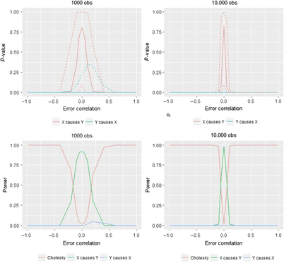
We first focus on whether we end up choosing the correct model using the model testing procedure outlined above — that is, we first estimate the Cholesky modelFootnote 10 and then see whether any of the alternative simpler models can be chosen without a significant reduction in fit as measured by likelihood-ratio tests. When the p value is above .05 for the correct model and the p value is below .05 for the alternative models, we end up selecting the correct model. For each of the values of the error correlation, we calculate the proportion of times the correct model is retained; this is our measure of power. This test can only be conducted in the case of the two unidirectional models (the first two presented in Table 1), as the reciprocal AE–CE model has the same degrees of freedom as the Cholesky AE–CE model. We therefore also compare all models — including the last model presented in Table 1, the reciprocal model — using AIC below, as suggested in the literature (Verhulst & Estabrook, Reference Verhulst and Estabrook2012).
In the results presented in Figure 6, the 95% confidence intervals are quite large in both the ‘small’ (1000 twin pairs) and ‘large’ (10,000 twin pairs) samples. Nonetheless, when there is zero non-shared confounding, we end up choosing the correct model on average for both sample sizes, and as shown in the bottom panels of Figure 6, this correct selection occurs frequently (i.e., power is above .8). However, as the amount of non-shared confounding increases, we very quickly lose the ability to choose the correct model. Instead, even with modest degrees of confounding, we are most likely to reject the true model and therefore to choose the Cholesky model, despite there being a quite strong causal effect of X on Y in this simulated data. This result is reflected in the two lower graphs which illustrate for a given sample size the model’s power, that is, the proportion of the time we select the correct model (i.e., the X → Y model). To gain a more complete understanding of the results, we also show the proportion that the other potential models are selected in these lower two panels of Figure 6. Most notably, when the sample size increases, the range of error-correlation values in which the true model is retained is even more restricted.
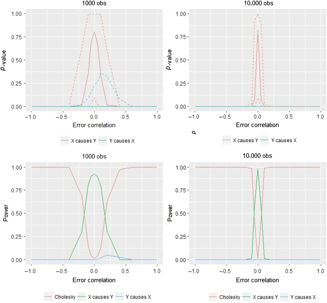
Fig. 6. Comparison of likelihood ratio tests in two sample size situations for AE–CE models and the corresponding power.
The situation is similar to using model chi-square to test the exact fit hypothesis in a classical structural equation modeling context: The larger the sample, the better able are we to detect even small differences between the population covariances (the DoC model instead uses the Cholesky model as its baseline) and the model-implied covariances, which in the DoC model testing framework are the various causal models outlined in Table 1 (Kline, Reference Kline2011). Put differently: When error correlations are non-zero, we are estimating the wrong model and the chi-square test therefore rejects it more quickly when the statistical power is more available to do so.
Numerical comparisons will help demonstrate the two main results of interest in Figure 6, namely the low amount of error correlation needed to affect the model choice and the stark degree to which sample size moderates these effects. As indicated in the lower panels of Figure 6, in a sample size of 1000, positive confounding of .1 or .2 leads to power of .79 and .31, respectively. With a sample of 10,000, these same amounts of positive confounding instead result in power of .01 and .00, respectively.
In cases where we have several alternative models, such as two unidirectional models or a reciprocal model with the same degrees of freedom as the Cholesky model, researchers have suggested using AIC for model selection; as always, the model with the lowest AIC is the preferred model. This is our second measure of power: the proportion of times for each of the values of the error correlation, we choose the correct model, that is, where the correct model has the lowest AIC. We only illustrate the interval [−.2, .2] in terms of confounding since otherwise it is impossible to display the variation in the AIC values across models since the AIC values at extreme amount of confounding decrease quite dramatically for most models, making the visualization difficult, also in the next figures where we present AIC values.Footnote 11 However, because the power graphs (in the lower panels of Figure 7) are still readily visualizable throughout the full range of error correlation values, we do not similarly restrict the range for the lower panels.
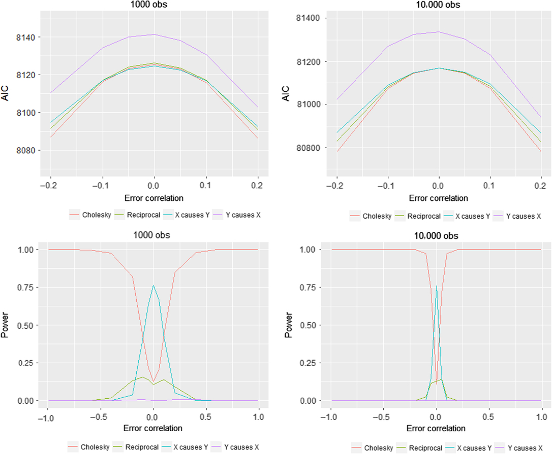
Fig. 7. Comparison of AIC values in two sample size situations for AE–CE models.
Although it is difficult to see in Figure 7, the model with the lowest AIC, both when the sample size is 1000 and 10,000, is the correct causal model where X causes Y. However, the differences between the univariate models and the reciprocal model are in many cases quite small. This is also illustrated by the power graphs. For instance, the power is about .76 when N = 1000 and when N = 10,000 in the case of zero confounding; that is, even under ideal conditions of zero error correlation, the DoC method will select one of the incorrect models a quarter of the time, irrespective of sample size. When the extent of confounding is even slightly different from zero, the Cholesky model has the lowest AIC value in most cases, and we would therefore have to choose this model, particularly when sample sizes are large. These results quite clearly demonstrate that even though there is a causal effect, the effect size is quite substantial, and there are very different modes of inheritance; in most cases, we would probably end up choosing an incorrect model — namely, the Cholesky.
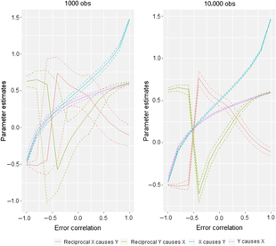
The final piece of the puzzle is the causal parameter estimates obtained from the different models, that is, i 1 and i 2 in Figure 1. This is illustrated in Figure 8. Recall that the true values for the simulation are X causing Y with an effect size of .5. Under conditions of no error correlation, the effect size is accurately estimated in both sample sizes, not only by the X causes Y model but also by the reciprocal model (which estimates an effect of .5 of X on Y and an effect of .0 of Y on X). Increases in the size of the error correlation do cause changes in the parameter estimates, but these might be considered less severe than the effects of error correlation on model selection: Considering the situation where non-shared confounding is −.2 — a situation in which our simulations showed the DoC often fails to select the appropriate model — the estimated median causal effect size in the 1000 observation case is .38. Thus, while the impact of modest to moderate degrees of non-shared confounding is quite destructive to the DoC’s ability to identify select the appropriate causal model, the impact on parameter estimates is closer to what researchers might generally expect in terms of changes in regression coefficients created by omitting relevant control variables.
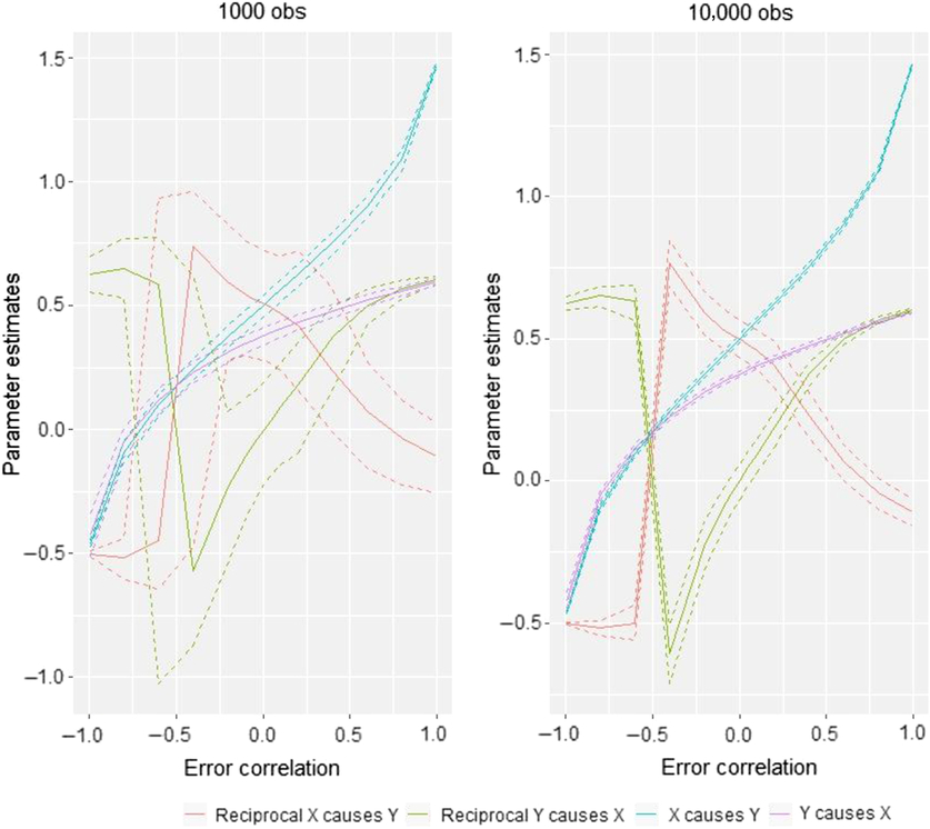
Fig. 8. Comparison of causal parameter estimates in two sample size situations for AE–CE models.
Conclusion and Discussion
The direction of causation model sought to solve one of the most intractable problems facing the scientific study of humans — the determination of causality. The use of the model is uneven across disciplines and research questions, but results on certain topics (such as personality and politics) results from the model are highly influential. The present study highlights how severe limitations in the model challenge its use in this and essentially all other domains.
This study first demonstrated analytically that unobserved non-shared confounding can bias parameter estimates and cross-twin, cross-trait covariances in the DoC model in twin research. We used this insight to conduct a series of simulation studies to investigate the effect non-shared confounding has on (1) choosing the correct causal model and (2) our (causal) parameter estimates. The results clearly demonstrate that in the face of even very small amounts of non-shared confounding, in even the best of situations — having two traits with widely different modes of heritability — the DoC leads to the choice of the wrong causal model. The parameter estimates are quite well recovered in both the models when we have zero confounding and we choose the correct model. However, we diverge from the population values when the extent of confounding increases and we choose the wrong model.
Appendix A (see Supplementary Material) outlines the results for the univariate ACE–ACE models, which closely match the variance components most often seen in the literature on many human characteristics, as well as the results for the corresponding reciprocal models. The details differ slightly from the results presented here, but the overall conclusion remains: In the face of often very slight amounts of non-shared confounding, we end up choosing the wrong model and estimate incorrect effect sizes. In addition, it is very difficult to use chi-squared testing to distinguish between unidirectional and reciprocal causation even in the face of zero confounding and 10,000 observations.
It is noteworthy that our present focus on non-shared confounding is, in fact, not the only way that the DoC could produce incorrect results through similar mechanisms. For example, response styles might represent a mechanism through which studies of self-reported characteristics would introduce an error correlation between the two characteristics under study, with similar consequences as a non-shared confounder. In fact, previous research on personality and politics has demonstrated just such an importance of response styles, further highlighting the challenges of using the technique in this particular domain (Kandler et al., Reference Kandler, Riemann, Spinath and Angleitner2010; Riemann & Kandler, Reference Riemann and Kandler2010). Creating measurement models to account for measurement error, as suggested by some DoC advocates (e.g., Verhulst & Estabrook, Reference Verhulst and Estabrook2012), is unfortunately not a solution to this problem as this approach would only account for random and not systematic measurement error such as that resulting from response styles.
Where does this leave us in terms of the use of using twin and family data for drawing causal inferences? A first thought is that the DoC model should be used cautiously and in limited situations. One appropriate situation for its use might be pure AE–CE models, where there is enough information to estimate the error correlation even in the reciprocal causation case.
Second, although the discordant twin design also suffers from problems of non-shared confounding (Frisell et al., Reference Frisell, Öberg, Kuja-Halkola and Sjölander2012), here, this is more a matter of biasing the parameter estimates rather than choosing the wrong model altogether; the discordant twin design compares MZ twins discordant on some exposure such as, for example, education. Thus, if a theoretical and/or empirical claim can be made with respect to the likelihood of non-shared confounding in a specific research setting, the discordant twin design still represents a strong research design for drawing causal inferences.
Finally, there are also other more advanced research designs that use genetic information to draw causal inferences, such as Mendelian randomization (Davey Smith & Ebrahim, Reference Davey Smith and Ebrahim2003), which is also a type of IV technique and which is arguably a stronger technique than the DoC model. There has been a recent attempt to integrate the DoC model and Mendelian randomization by Minică et al. (Reference Minică, Dolan, Boomsma, de Geus and Neale2018). The Mendelian randomization approach to reducing unobserved confounding is an improvement to DOC modeling. The problem of non-shared confounding is not resolved, however, using this approach, as the authors also note (Minică et al., Reference Minică, Dolan, Boomsma, de Geus and Neale2018). Even if one has a valid instrument, effects accumulating over time (since birth) due to selection are potential sources of latent confounding. Just how sensitive this alternative approach is to non-shared confounding needs to be investigated further.
Supplementary Material
To view supplementary material for this article, please visit https://doi.org/10.1017/thg.2018.67.
Acknowledgment
We would like to thank Asbjørn Sonne Nørgaard, Robert Klemmensen and Matt McGue for support in writing this article.
Financial Support
None.
Conflict of Interest
We have a conflict of interest with Pete Hatemi and Brad Verhulst because of this publication: Ludeke, S. G. & Rasmussen, S. H. R. (2016). Personality correlates of sociopolitical attitudes in the Big Five and Eysenckian models. Personality and Individual Differences, 98, 30–36.
Ethical Standards
The study did not involve human participants or animals and therefore does not require informed consent or compliance with any ethical standards research guidelines.