


1. Introduction
Inertial measurement units (IMUs) have gained significant interest in recent years as a wearable tool for quantifying human movement. These systems are wireless, wearable, noninvasive and can provide real-time data, making them a potential alternative to traditional motion capture methods such as optical systems. This technique is particularly used for monitoring the kinematics of the body’s articulated structures composed of rigid segments (limbs or body parts) connected by joints (articulations). In such applications, one IMU per segment is used for several applications, such as biomechanics, ergonomics, and sports (Baklouti et al., Reference Baklouti, Chaker, Rezgui, Sahbani, Bennour and Laribi2024; Fain et al., Reference Fain, McCarthy, Nindl, Fuller, Wills and Doyle2024; Vigne et al., Reference Vigne, Khoury, Meglio and Petit2020). This approach also comes with several challenges, such as the random nature of movements due to high number of degrees of freedom and variable dynamics, which eliminate the possibility of relying on movement patterns to improve motion estimation.
The fusion of gyroscope, accelerometer, and magnetometer data enables the estimation of joint angles in articulated structures. Data from the magnetometer help to identify the system’s orientation relative to the Earth’s magnetic north, necessitating adequate calibration. Thus, the reliability of joint angle estimation becomes dependent on the magnetometer data and adequate calibration procedures, which limit system versatility. Indoor environments containing ferromagnetic materials and electronic devices can distort the local magnetic field, leading to orientation errors (Fan et al., Reference Fan, Li and Liu2017; Laidig and Seel, Reference Laidig and Seel2023).
Such magnetic disturbances compromise the accuracy and reliability of orientation data, making magnetometer-dependent systems less robust in real-world conditions (Rogers et al., Reference Rogers, Costello, Harkins and Hamaoui2011). Furthermore, magnetometer calibration is a complex and time-consuming process that often requires specialized equipment and procedures. Even after calibration, magnetometer performance remains highly sensitive to prolonged use and variations in the surrounding magnetic environment (Yadav and Bleakley, Reference Yadav and Bleakley2014). This further highlights the need for methods that can provide consistent and accurate orientation estimates without relying on the magnetic field.
To address these challenges, current research has explored sensor fusion techniques that exclude magnetometers. These approaches often employ advanced algorithms to integrate data from multiple gyroscope and accelerometer sensors and estimate orientation accurately. Madgwick et al. (Reference Madgwick, Harrison and Vaidyanathan2011) developed a gradient descent algorithm that uses accelerometer data to correct gyroscope measurements. This is achieved by iteratively minimizing the error between estimated and measured accelerations to refine orientation estimates. In addition, Kim and Golnaraghi (Reference Kim and Golnaraghi2004) present a quaternion-based KF for orientation estimation using only gyroscope and accelerometer data. Their method avoids the use of magnetometers by relying on the relationship between the quaternion representing the platform orientation and the measurements of gravity from the accelerometers, combined with angular rate measurements from the gyros. This approach demonstrated accurate and stable orientation estimates over long periods without the need for magnetometers (Kim and Golnaraghi, Reference Kim and Golnaraghi2004). Similarly, the versatile quaternion-based filter (VQF) algorithm proposed by Laidig and Seel (Reference Laidig and Seel2023) utilizes a quaternion-based orientation estimation algorithm that integrates gyroscope and accelerometer data. This approach includes a novel filtering technique for acceleration measurements and incorporates gyroscope bias estimation to enhance accuracy, outperforming eight other literature methods (Laidig and Seel, Reference Laidig and Seel2023).
Despite these advancements, several critical gaps in orientation estimation methods remain unaddressed. The gradient descent method proposed by Madgwick et al., Reference Madgwick, Harrison and Vaidyanathan2011, for example, relies on initial assumptions that may not hold across various environments. Similarly, the method by Kim and Golnaraghi (Reference Kim and Golnaraghi2004) is based on the premise of stable and predictable motion patterns, which are often not present in dynamic or complex environments, such as human motion analysis. This can lead to significant errors, resulting in unreliable orientation estimates under challenging conditions (Bernal-Polo and Martínez Barberá, Reference Bernal-Polo and Martínez Barberá2017). Additionally, the VQF algorithm, noted for its high accuracy (Laidig and Seel, Reference Laidig and Seel2023), requires meticulous parameter tuning and considerable computational resources. This may hinder its deployment in real-time applications on devices with limited processing power. This algorithm also assumes specific characteristics of magnetic disturbances and motion dynamics, potentially limiting its effectiveness in diverse real-world scenarios. Furthermore, Zihajehzadeh and Park (Reference Zihajehzadeh and Park2017) have highlighted the challenges faced by various magnetometer-free filters, particularly in maintaining long-term stability and accurate yaw estimation. These filters struggle to completely eliminate drift without magnetometer data, impacting their effectiveness. While accelerometers perform well in correcting roll and pitch orientations (Łuczak et al., Reference Łuczak, Zams, Dąbrowski and Kusznierewicz2022), they face difficulties with yaw angle corrections (Kim and Golnaraghi, Reference Kim and Golnaraghi2004). Traditional yaw measurements utilize magnetometers to detect the Earth’s magnetic field direction (Xiaoping et al., Reference Xiaoping, Bachmann and McGhee2008); however, accelerometers, which measure linear acceleration and gravitational forces, do not directly inform about the heading relative to the magnetic field (Halitim et al., Reference Halitim, Bouhedda, Tchoketch-Kebir and Rebouh2023), further complicating accurate orientation estimation using accelerometer data alone.
This study addresses these identified research gaps by developing sensor fusion algorithms adapted to varying environments for human body joint angle estimation with minimal manual calibration. The focus is on an adaptive orientation estimation method that functions effectively across diverse motion directions and dynamics without requiring extensive calibration processes. Moreover, the approach is designed to be robust in environments with fluctuating magnetic fields, ensuring reliable performance even in the presence of magnetic disturbances.
Specifically, the research introduces a novel magnetometer-free approach that uses the Kalman filter to enhance orientation estimation by analyzing the accelerometer’s alignment with the Earth’s frame. This method’s accuracy is assessed against well-known algorithms, such as complementary filters and a DSKF, and benchmarked against a reference sensor solution. Additionally, the study evaluates the practical application of this method in upper limb motion monitoring. Comparisons are made with a standard motion capture system to test the method’s integration and effectiveness in real-world scenarios. Through statistical analysis, the study seeks to identify differences between the systems and determine the factors that impact the accuracy of IMU-based measurements, thereby offering potential improvements in sensor fusion technology for dynamic and complex environments.
2. Methods
2.1. Proposed magnetometer-free orientation estimation approach design
The primary objective of the proposed algorithm is to estimate the orientation of wearable IMUs in environments prone to magnetic interference. Figure 1 showcases a simplified block diagram of the proposed orientation estimation algorithm.
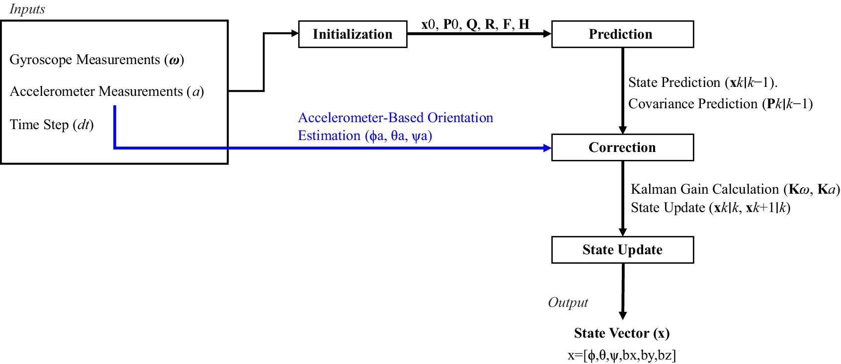
Figure 1. Simplified block diagram of the proposed orientation estimation algorithm for wearable IMUs.
The inputs for the algorithm include:
-
• Gyroscope measurements $ \omega $
, representing angular velocity readings along the three axes (X, Y, Z).
$ \omega $
, representing angular velocity readings along the three axes (X, Y, Z). -
• Accelerometer measurements
$ \mathbf{a} $
, providing acceleration readings along the three axes (X, Y, Z). -
• The time step
$ dt $
, representing the sampling interval between consecutive measurements. -
• The output of the algorithm is the state vector
$ \mathbf{x} $
(Equation 2.1). It includes: -
• Orientation angles (roll
$ \phi $
, pitch
$ \theta $
, yaw
$ \psi $
) relative to the Earth’s frame. -
• Corrected gyroscope biases (
$ {b}_x $
,
$ {b}_y $
,
$ {b}_z $
) along the three axes (X, Y, Z), accounting for errors in gyroscope readings.


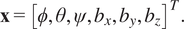 $$ \mathbf{x}={\left[\phi, \theta, \psi, {b}_x,{b}_y,{b}_z\right]}^T. $$
The proposed algorithm utilizes a refined Kalman filter (KF) framework to fuse sensor data in three iterative steps: initialization, prediction, and correction. These steps estimate the orientation angles and correct gyroscope drift.
The algorithm begins by setting the initial values of the parameters, which are empirically tuned based on sensor noise statistics and system requirements:
-
• An initial
$ 6\times 1 $
state vector (
$ {\mathbf{x}}_{\mathbf{0}} $
) that represents the system’s initial orientation (roll ϕ, pitch
$ \theta $
, yaw
$ \psi $
) and gyroscope biases (
$ {b}_x $
,
$ {b}_y $
,
$ {b}_z $
). Initially, all elements of this vector are set to zero, assuming no prior knowledge of the orientation or biases. -
• An initial
$ 6\times 6 $
symmetric state covariance matrix (
$ {\mathbf{P}}_0 $
) that captures the uncertainty in the state estimates. Each entry quantifies the variance or covariance of state variables, derived from the standard deviations (stds) of roll, pitch, yaw, and gyroscope biases. This matrix is initialized based on the expected noise characteristics of the sensors. -
• A
$ 6\times 6 $
process noise covariance matrix (
$ \mathbf{Q} $
) that models uncertainty in the state prediction due to sensor noise characteristics. -
• A
$ 3\times 3 $
diagonal measurement noise covariance matrix (
$ \mathbf{R} $
) that characterizes sensor noise during the correction step. -
• A
$ 6\times 6 $
state transition matrix (
$ \mathbf{F} $
) that models the evolution of the state over time. It incorporates angular velocity integration and gyroscope bias dynamics, with the parameter
$ dt $
representing the sampling interval between measurements. -
• A
$ 3\times 6 $
measurement matrix (
$ \mathbf{H} $
) that maps the state vector to the estimated tilt angles. It extracts the relevant components of the state vector (roll, pitch, and yaw) for comparison with sensor data.


In the prediction step, the state $ \mathbf{x} $
and covariance
$ \mathbf{x} $
and covariance $ \mathbf{P} $
are projected forward using the state transition matrix
$ \mathbf{P} $
are projected forward using the state transition matrix $ \mathbf{F} $
and process noise covariance
$ \mathbf{F} $
and process noise covariance $ \mathbf{Q} $
, as described in Equations (2.2) and (2.3):
$ \mathbf{Q} $
, as described in Equations (2.2) and (2.3):
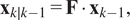 $$ {\mathbf{x}}_{k\mid k-1}=\mathbf{F}\cdot {\mathbf{x}}_{k-1}, $$
 $$ {\mathbf{P}}_{k\mid k-1}=\mathbf{F}\cdot {\mathbf{P}}_{k-1}\cdot {\mathbf{F}}^T+\mathbf{Q}. $$
The proposed method determines orientations from accelerometer data by aligning the sensor frame with the global Cartesian frame (Earth’s frame), enabling the correction of gyroscope drift. When static, accelerometer readings reflect the projection of gravity ( $ \mathbf{g} $
) along its axes. A rotation matrix
$ \mathbf{g} $
) along its axes. A rotation matrix $ {\mathbf{R}}_{\mathrm{align}} $
aligns the sensor frame with the global frame, as given in Equations (2.4) and (2.5):
$ {\mathbf{R}}_{\mathrm{align}} $
aligns the sensor frame with the global frame, as given in Equations (2.4) and (2.5):
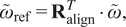 $$ {\tilde{\omega}}_{\mathrm{ref}}={\mathbf{R}}_{\mathrm{align}}^T\cdot \tilde{\omega}, $$
 $$ {\tilde{\mathbf{a}}}_{\mathrm{ref}}={\mathbf{R}}_{\mathrm{align}}^T\cdot \tilde{\mathbf{a}}. $$
Here, $ {\tilde{\omega}}_{\mathrm{ref}} $
and
$ {\tilde{\omega}}_{\mathrm{ref}} $
and $ {\tilde{\mathbf{a}}}_{\mathrm{ref}} $
represent angular velocity and acceleration in the Earth’s reference frame, respectively, while
$ {\tilde{\mathbf{a}}}_{\mathrm{ref}} $
represent angular velocity and acceleration in the Earth’s reference frame, respectively, while $ \tilde{\omega} $
and
$ \tilde{\omega} $
and $ \tilde{\mathbf{a}} $
represent their respective values in the sensor frame.
$ \tilde{\mathbf{a}} $
represent their respective values in the sensor frame.
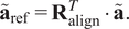
By aligning the IMU sensor frame with the Earth’s reference frame, the algorithm computes the accelerometer’s orientation angles ( $ {\phi}_a $
,
$ {\phi}_a $
, $ {\theta}_a $
,
$ {\theta}_a $
, $ {\psi}_a $
, illustrated in Figure 2) relative to the Earth’s axes:
$ {\psi}_a $
, illustrated in Figure 2) relative to the Earth’s axes:
-
•
$ {\phi}_a $
(roll): Rotation about the Earth’s X-axis. -
•
$ {\theta}_a $
(pitch): Rotation about the Earth’s Y-axis. -
•
$ {\psi}_a $
: Angle between the IMU’s Z-axis and the gravity vector, serving as yaw approximation.


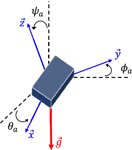
Figure 2. Schematic illustration of the accelerometer-derived inclination angles.
These angles (Eqs. 2.6–2.8) are derived from transformed accelerometer measurements $ {\tilde{\mathbf{a}}}_{\mathrm{ref}}=\left({\tilde{a}}_{\mathrm{ref},x},{\tilde{a}}_{\mathrm{ref},y},{\tilde{a}}_{\mathrm{ref},z}\right) $
(Fisher, Reference Fisher2010; Pedley, Reference Pedley2013). In upper limb motion analysis, this yaw approximation is particularly effective in biomechanically constrained scenarios due to anatomical coupling. Movements such as shoulder elevation or forearm rotation inherently alter the IMU’s inclination relative to gravity, correlating with task-specific orientation changes.
$ {\tilde{\mathbf{a}}}_{\mathrm{ref}}=\left({\tilde{a}}_{\mathrm{ref},x},{\tilde{a}}_{\mathrm{ref},y},{\tilde{a}}_{\mathrm{ref},z}\right) $
(Fisher, Reference Fisher2010; Pedley, Reference Pedley2013). In upper limb motion analysis, this yaw approximation is particularly effective in biomechanically constrained scenarios due to anatomical coupling. Movements such as shoulder elevation or forearm rotation inherently alter the IMU’s inclination relative to gravity, correlating with task-specific orientation changes.
 $$ {\phi}_{\mathrm{a}}=\arctan 2\left(\frac{{\tilde{a}}_{\mathrm{ref},y}}{\sqrt{{\tilde{a}}_{\mathrm{ref},x}^2+{\tilde{a}}_{\mathrm{ref},z}^2}}\right) $$
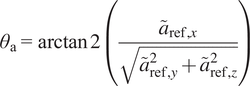 $$ {\theta}_{\mathrm{a}}=\arctan 2\left(\frac{{\tilde{a}}_{\mathrm{ref},x}}{\sqrt{{\tilde{a}}_{\mathrm{ref},y}^2+{\tilde{a}}_{\mathrm{ref},z}^2}}\right) $$
 $$ {\psi}_{\mathrm{a}}=\arctan 2\left(\frac{\sqrt{{\tilde{a}}_{\mathrm{ref},x}^2+{\tilde{a}}_{\mathrm{ref},y}^2}}{{\tilde{a}}_{\mathrm{ref},z}}\right) $$
Following this, an update step refines estimates using gyroscope data, as described in Equations (2.9) and (2.10). Here, $ {\mathbf{H}}_{\omega } $
maps the state vector to gyroscope measurements, and
$ {\mathbf{H}}_{\omega } $
maps the state vector to gyroscope measurements, and $ {\mathbf{R}}_{\omega } $
characterizes gyroscope noise.
$ {\mathbf{R}}_{\omega } $
characterizes gyroscope noise.
 $$ {\mathbf{K}}_{\omega }={\mathbf{P}}_{k\mid k-1}\cdot {\mathbf{H}}_{\omega}^T\cdot {\left({\mathbf{H}}_{\omega}\cdot {\mathbf{P}}_{k\mid k-1}\cdot {\mathbf{H}}_{\omega}^T+{\mathbf{R}}_{\omega}\right)}^{-1} $$
 $$ {\mathbf{x}}_{k\mid k}={\mathbf{x}}_{k\mid k-1}+{\mathbf{K}}_{\omega}\cdot \left({\omega}_k-{\mathbf{H}}_{\omega}\cdot {\mathbf{x}}_{k\mid k-1}\right) $$
Finally, the accelerometer-derived angles correct the state estimate via Equations (2.11) and (2.12). Here, $ {\mathbf{H}}_a $
maps the state vector to accelerometer measurements, and
$ {\mathbf{H}}_a $
maps the state vector to accelerometer measurements, and $ {\mathbf{R}}_a $
characterizes accelerometer noise. By fusing accelerometer-derived angles with gyroscope data, the algorithm corrects gyroscope drift across all three axes.
$ {\mathbf{R}}_a $
characterizes accelerometer noise. By fusing accelerometer-derived angles with gyroscope data, the algorithm corrects gyroscope drift across all three axes.
 $$ {\mathbf{K}}_a={\mathbf{P}}_{k\mid k}\cdot {\mathbf{H}}_a^T\cdot {\left({\mathbf{H}}_a\cdot {\mathbf{P}}_{k\mid k}\cdot {\mathbf{H}}_a^T+{\mathbf{R}}_a\right)}^{-1} $$
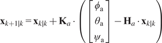 $$ {\mathbf{x}}_{k+1\mid k}={\mathbf{x}}_{k\mid k}+{\mathbf{K}}_a\cdot \left(\left[\begin{array}{c}{\phi}_{\mathrm{a}}\\ {}{\theta}_{\mathrm{a}}\\ {}{\psi}_{\mathrm{a}}\end{array}\right]-{\mathbf{H}}_a\cdot {\mathbf{x}}_{k\mid k}\right) $$
The Kalman gain matrices ( $ {\mathbf{K}}_{\omega } $
and
$ {\mathbf{K}}_{\omega } $
and $ {\mathbf{K}}_a $
) weight the contributions of gyroscope and accelerometer data, ensuring optimal fusion of sensor inputs.
$ {\mathbf{K}}_a $
) weight the contributions of gyroscope and accelerometer data, ensuring optimal fusion of sensor inputs.
2.2. Upper limb kinematics estimation from IMU data
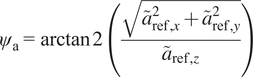
To transform the orientation data from IMU sensors into joint angles, this study models the kinematics of the upper extremity, focusing on the shoulder, elbow, and wrist joints, as illustrated in Figure 3.
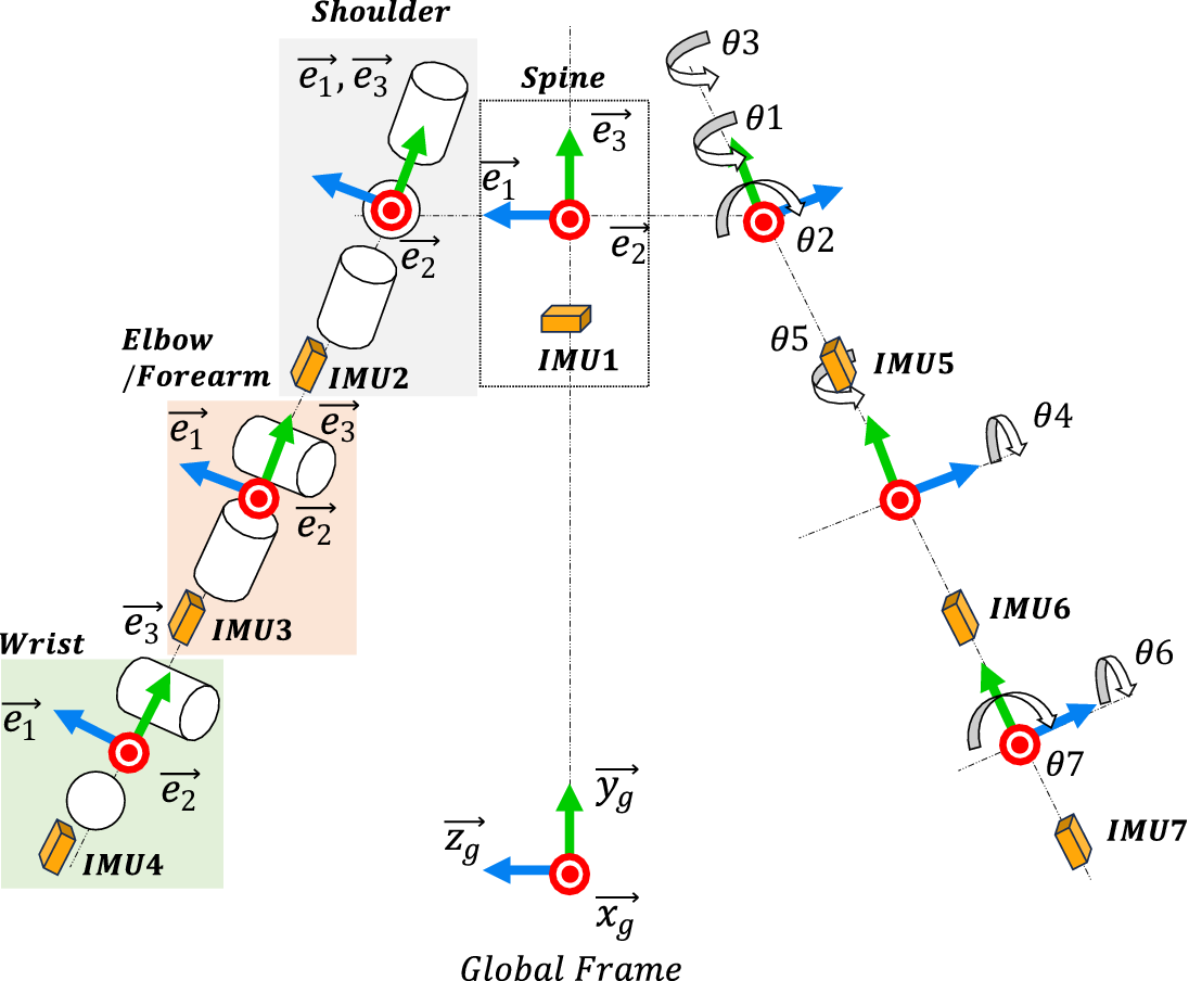
Figure 3. Representation of upper body kinematics, including the spine and upper limbs.
Initially, the IMU sensors are aligned with the Earth frame. This alignment ensures that the sensor frames are consistent with the anatomical frames. The relative quaternion, $ {\mathbf{q}}_{\mathrm{relative}} $
, between two consecutive segments represents joint variations due to movement, as shown in Equation (2.13). Here,
$ {\mathbf{q}}_{\mathrm{relative}} $
, between two consecutive segments represents joint variations due to movement, as shown in Equation (2.13). Here, $ {\mathbf{q}}_1 $
and
$ {\mathbf{q}}_1 $
and $ {\mathbf{q}}_2 $
represent the orientations of the first and second segments, respectively.
$ {\mathbf{q}}_2 $
represent the orientations of the first and second segments, respectively.
 $$ {\mathbf{q}}_{\mathrm{relative}}={\mathbf{q}}_1^{-1}\cdot {\mathbf{q}}_2 $$
The joint angles are defined as rotations around the X, Y, and Z axes. Depending on the rotation sequence, joint angles $ {\theta}_x $
,
$ {\theta}_x $
, $ {\theta}_y $
, and
$ {\theta}_y $
, and $ {\theta}_z $
are estimated from the quaternions. For each joint, quaternions are calculated based on their respective Euler sequences:
$ {\theta}_z $
are estimated from the quaternions. For each joint, quaternions are calculated based on their respective Euler sequences:
-
• For the shoulder joint,
$ {\mathbf{q}}_{\mathrm{shoulder}} $
is computed using the Y-X-Z rotation order, considering the thorax and upper arm segments. -
• For the elbow joint,
$ {\mathbf{q}}_{\mathrm{elbow}} $
is computed using the X-Z-Y rotation order, considering the upper arm and forearm segments. -
• For the wrist joint,
$ {\mathbf{q}}_{\mathrm{wrist}} $
is computed using the X-Y-Z rotation order, considering the forearm and hand segments.


These computations assume the shoulder is initially abducted $ {90}^{\circ } $
in the frontal plane and the forearm is fully pronated.
$ {90}^{\circ } $
in the frontal plane and the forearm is fully pronated.
Given $ {\mathbf{q}}_{\mathrm{relative}}=\left[{q}_w,{q}_x,{q}_y,{q}_z\right] $
, the joint angles are calculated as shown in Equations (2.14)–(2.16). Here,
$ {\mathbf{q}}_{\mathrm{relative}}=\left[{q}_w,{q}_x,{q}_y,{q}_z\right] $
, the joint angles are calculated as shown in Equations (2.14)–(2.16). Here, $ {\theta}_1 $
represents flexion/extension,
$ {\theta}_1 $
represents flexion/extension, $ {\theta}_2 $
represents abduction/adduction, and
$ {\theta}_2 $
represents abduction/adduction, and $ {\theta}_3 $
represents internal/external rotation of the shoulder joint.
$ {\theta}_3 $
represents internal/external rotation of the shoulder joint.
 $$ {\theta}_1=\arcsin \left(2\left({q}_w{q}_x-{q}_y{q}_z\right)\right) $$
 $$ {\theta}_2=\arctan 2\left(2\left({q}_x{q}_z-{q}_w{q}_y\right),\left({q}_w^2-{q}_x^2-{q}_y^2+{q}_z^2\right)\right) $$
 $$ {\theta}_3=\arctan 2\left(2\left({q}_x{q}_y+{q}_w{q}_z\right),\left({q}_w^2-{q}_x^2+{q}_y^2-{q}_z^2\right)\right) $$
For the elbow joint, the joint angles are calculated as shown in Equations (2.17)–(2.18). Here, $ {\theta}_4 $
represents flexion/extension, and
$ {\theta}_4 $
represents flexion/extension, and $ {\theta}_5 $
represents pronation-supination rotation.
$ {\theta}_5 $
represents pronation-supination rotation.
 $$ {\theta}_4=\arctan 2\left(2\left({q}_w{q}_x+{q}_y{q}_z\right),\left({q}_w^2-{q}_x^2+{q}_y^2-{q}_z^2\right)\right) $$
 $$ {\theta}_5=\arctan 2\left(2\left({q}_w{q}_y+{q}_x{q}_z\right),\left({q}_w^2+{q}_x^2-{q}_y^2-{q}_z^2\right)\right) $$
For the wrist joint, the joint angles are calculated as shown in Equations (2.19)–(2.20). Here, $ {\theta}_6 $
represents flexion/extension, and
$ {\theta}_6 $
represents flexion/extension, and $ {\theta}_7 $
represents adduction/abduction.
$ {\theta}_7 $
represents adduction/abduction.
 $$ {\theta}_6=\arctan 2\left(-2\left({q}_y{q}_z-{q}_w{q}_x\right),\left(1-2\left({q}_x^2+{q}_y^2\right)\right)\right) $$
 $$ {\theta}_7=\arctan 2\left(-2\left({q}_x{q}_y-{q}_w{q}_z\right),\left(1-2\left({q}_y^2+{q}_z^2\right)\right)\right) $$
2.3. Experimental setup for the evaluation of the proposed method
The evaluation of the proposed algorithm for sensor orientation estimation is conducted in two distinct phases. In Phase 1, the algorithm’s performance is assessed against renowned sensor fusion algorithms using controlled robotic movements. In Phase 2, the algorithm is tested in a real-world scenario using a wearable IMU-based system for human motion analysis. The 9-degree of freedom (DoF) MPU-9250 micro-electromechanical systems (MEMS)-based IMU used in this study includes: A 3-axis accelerometer ( $ \pm 16\hskip0.1em g $
range), a 3-axis gyroscope (
$ \pm 16\hskip0.1em g $
range), a 3-axis gyroscope ( $ \pm {2000}^{\circ }/\mathrm{s} $
range), and a 3-axis magnetometer (
$ \pm {2000}^{\circ }/\mathrm{s} $
range), and a 3-axis magnetometer ( $ \pm 4800\hskip0.22em \unicode{x03BC} \mathrm{T} $
range). This sensor was employed in both the controlled robotic experiments and the human motion analysis trials.
$ \pm 4800\hskip0.22em \unicode{x03BC} \mathrm{T} $
range). This sensor was employed in both the controlled robotic experiments and the human motion analysis trials.
2.3.1. Phase 1: Controlled environment testing
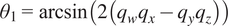
In Phase 1, the 9-DoF IMU is mounted on the end effector of a 5-axis SCORBOT ER-9 PRO robot. The X-, Y-, and Z-axes of the sensor are aligned with those of the robot (Figure 4), ensuring that the IMU’s orientation accurately reflects the rotational motions of the robot’s end effector. The setup, connected to an ARDUINO Mega2560 microcontroller, facilitates the capture of rotation data around the three axes of the sensor. A total of 20 repetitions are performed for each rotational axis to evaluate the algorithm’s accuracy.
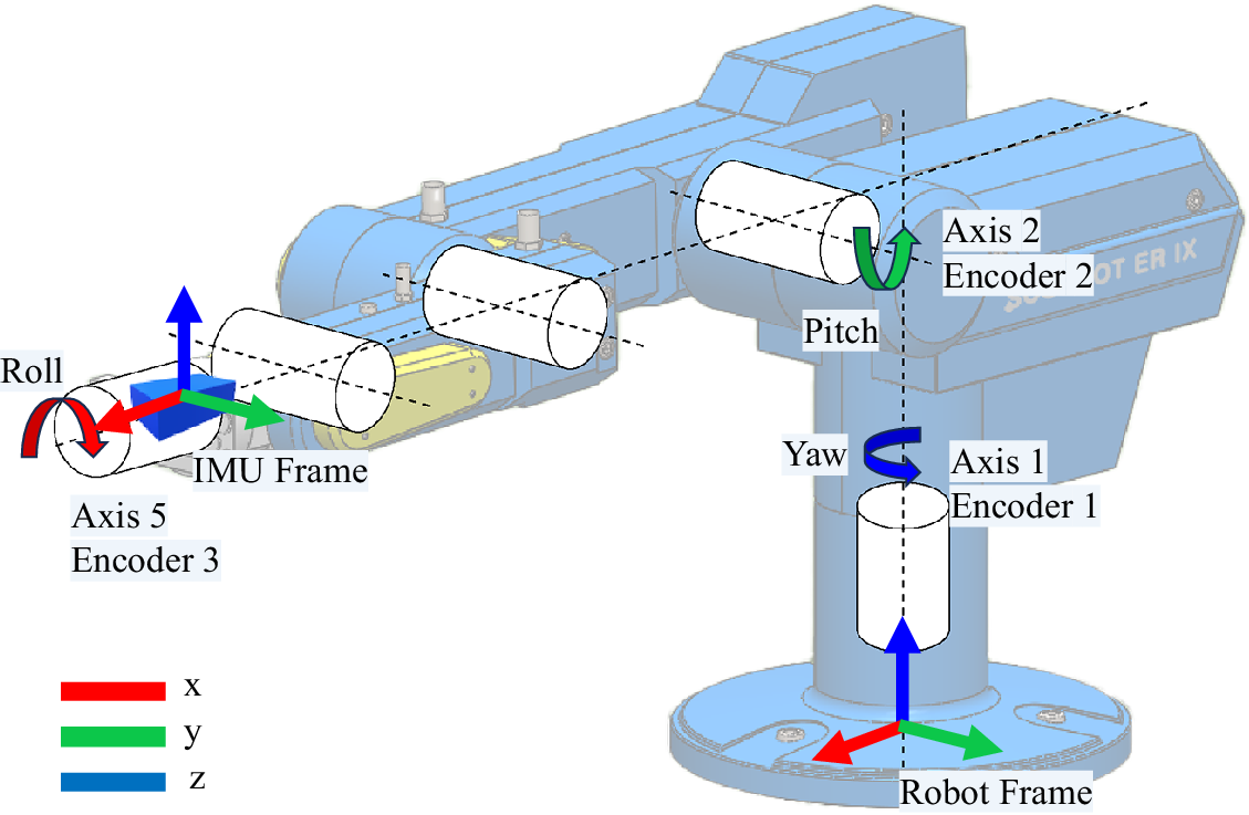
Figure 4. Experimental setup with the MPU-9250 IMU mounted on the SCORBOT ER-9 PRO robot.
2.3.2. Phase 2: Human motion analysis
The second phase involves implementing the algorithm in a wearable IMU-based system for upper limb motion capture. The system comprises seven IMU nodes attached to the upper arm, forearm, and hand segments, operating at a sample rate of $ 10\hskip0.22em \mathrm{Hz} $
. Three healthy female volunteers (age:
$ 10\hskip0.22em \mathrm{Hz} $
. Three healthy female volunteers (age: $ 28\pm 2 $
years; height:
$ 28\pm 2 $
years; height: $ 167\pm 3.5 $
cm; weight:
$ 167\pm 3.5 $
cm; weight: $ 65.5\pm 3 $
kg) participated in the acquisition session. They were equipped with wearable sensors and 28 reflective markers. The 3D trajectories of the markers were collected at
$ 65.5\pm 3 $
kg) participated in the acquisition session. They were equipped with wearable sensors and 28 reflective markers. The 3D trajectories of the markers were collected at $ 100\hskip0.22em \mathrm{Hz} $
using a Vicon Optical Motion Capture (OMC) system with 38 cameras (Vicon, Oxford Metrics Ltd, Oxford, UK).
$ 100\hskip0.22em \mathrm{Hz} $
using a Vicon Optical Motion Capture (OMC) system with 38 cameras (Vicon, Oxford Metrics Ltd, Oxford, UK).
After a 30-s T-pose for calibration, participants performed 10 repetitions of upper body movements representing the key degrees of freedom. These included: 3 movements at the shoulder: $ {\theta}_1 $
(flexion/extension),
$ {\theta}_1 $
(flexion/extension), $ {\theta}_2 $
(abduction/adduction), and
$ {\theta}_2 $
(abduction/adduction), and $ {\theta}_3 $
(internal/external rotation); two movements at the elbow:
$ {\theta}_3 $
(internal/external rotation); two movements at the elbow: $ {\theta}_4 $
(flexion/extension) and
$ {\theta}_4 $
(flexion/extension) and $ {\theta}_5 $
(pronation/supination); and two movements at the wrist:
$ {\theta}_5 $
(pronation/supination); and two movements at the wrist: $ {\theta}_6 $
(flexion/extension) and
$ {\theta}_6 $
(flexion/extension) and $ {\theta}_7 $
(radial/ulnar deviation). The aim was to measure the movements within each DoF individually.
$ {\theta}_7 $
(radial/ulnar deviation). The aim was to measure the movements within each DoF individually.
Data from both systems were compared to assess the validity of the IMU-based system against the gold standard OMC system. The data obtained from the OMC system were processed using the Plugin-Gait (PiG) upper body model for kinematic calculations, as illustrated in Figure 5.
Figure 5. Visual representation of the experimental setup: (a) schematic Illustration and (b) real-life experimental setup of IMU-based and OMC-based systems.
2.4. Data analysis
2.4.1. Error analysis compared to encoders and filtering techniques
IMU sensor calibration, orientation estimation, and encoder measurement calculations were performed according to the study by Baklouti et al. (Reference Baklouti, Rezgui, Chaouch, Chaker, Mefteh, Sahbani, Bennour, Walha, Jarraya, Djemal, Chouchane, Aifaoui, Chaari, Abdennadher, Benamara and Haddar2022). Statistical measures were used to compare the IMU system’s performance against the robot’s reference encoder measurements (considered as the ground truth). Additionally, comparisons were made with the DSKF and complementary filter for orientation estimation around the X, Y, and Z-axes.
The DSKF, as described in Sabatelli et al. (Reference Sabatelli, Galgani, Fanucci and Rocchi2013), employs a two-step correction process for orientation estimation using quaternions. During the first stage, roll and pitch angles are corrected by comparing the expected and measured gravity vectors from the accelerometer. In the second stage, the yaw angle is refined using magnetometer data.
The complementary filter integrates the high-frequency response of gyroscope data with the low-frequency response of accelerometer and magnetometer data. It uses the accelerometer to correct roll and pitch angles and the magnetometer to correct the yaw angle. The filter is formulated as shown in Equation (2.21):
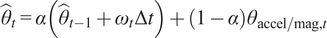 $$ {\hat{\theta}}_t=\alpha \left({\hat{\theta}}_{t-1}+{\omega}_t\Delta t\right)+\left(1-\alpha \right){\theta}_{\mathrm{accel}/\mathrm{mag},t} $$
where $ {\hat{\theta}}_t $
is the estimated orientation at time
$ {\hat{\theta}}_t $
is the estimated orientation at time $ t $
,
$ t $
, $ {\hat{\theta}}_{t-1} $
is the estimated orientation at the previous time step,
$ {\hat{\theta}}_{t-1} $
is the estimated orientation at the previous time step, $ {\omega}_t $
is the angular rate measured by the gyroscope,
$ {\omega}_t $
is the angular rate measured by the gyroscope, $ \Delta t $
is the time step,
$ \Delta t $
is the time step, $ {\theta}_{\mathrm{accel}/\mathrm{mag},t} $
is the orientation calculated from the accelerometer and magnetometer data, and
$ {\theta}_{\mathrm{accel}/\mathrm{mag},t} $
is the orientation calculated from the accelerometer and magnetometer data, and $ \alpha $
is the filter gain, typically chosen to balance the contributions of the gyroscope and accelerometer/magnetometer. In this study,
$ \alpha $
is the filter gain, typically chosen to balance the contributions of the gyroscope and accelerometer/magnetometer. In this study, $ \alpha =0.9 $
.
$ \alpha =0.9 $
.
The metrics utilized included the correlation coefficient $ (r) $
, which indicates the linear relationship strength and direction between the IMU and encoder measurements; the coefficient of determination
$ (r) $
, which indicates the linear relationship strength and direction between the IMU and encoder measurements; the coefficient of determination $ \left({r}^2\right) $
, representing the variance proportion in encoder measurements explained by the IMU data; RMSE, measuring the average magnitude of errors; intra-class correlation coefficient (ICC, two-way mixed effects), assessing the measurement reliability and consistency; lower limit of agreement (LoA), providing the range capturing most differences between IMU and encoder measurements, indicating agreement; mean absolute error (MAE), computing the average absolute differences; and normalized mean bias error (NMBE), reflecting the average bias of the IMU measurements relative to the encoders.
$ \left({r}^2\right) $
, representing the variance proportion in encoder measurements explained by the IMU data; RMSE, measuring the average magnitude of errors; intra-class correlation coefficient (ICC, two-way mixed effects), assessing the measurement reliability and consistency; lower limit of agreement (LoA), providing the range capturing most differences between IMU and encoder measurements, indicating agreement; mean absolute error (MAE), computing the average absolute differences; and normalized mean bias error (NMBE), reflecting the average bias of the IMU measurements relative to the encoders.
2.4.2. Kinematic analysis using statistical parametric mapping
To assess the agreement between IMU and VICON (considered as the ground truth) measurements, a set of metrics was employed, including RMSE, MAE, NMBE, and $ {r}^2 $
. These metrics were further contextualized by considering the ROM for each joint, allowing for a more nuanced interpretation of the error measures. To statistically evaluate potential differences between IMU and VICON measurements for each DoF, a curve analysis was performed using statistical parametric mapping (SPM) with a two-tailed paired t-test (Flandin and Friston, Reference Flandin and Friston2008). This analysis included a two-tailed paired t-test to compare joint angles from both systems, setting a significance level at
$ {r}^2 $
. These metrics were further contextualized by considering the ROM for each joint, allowing for a more nuanced interpretation of the error measures. To statistically evaluate potential differences between IMU and VICON measurements for each DoF, a curve analysis was performed using statistical parametric mapping (SPM) with a two-tailed paired t-test (Flandin and Friston, Reference Flandin and Friston2008). This analysis included a two-tailed paired t-test to compare joint angles from both systems, setting a significance level at $ \alpha =0.05 $
. Data were synchronized and time normalized within MATLAB after aligning to the first movement peak, formatted into 101 data points (0–100%). The SPM{t} statistic was computed at each time node to determine the level of similarity between the curves. Regions where SPM{t} exceeded the critical t-value, indicating statistically significant differences, were identified and analyzed to pinpoint phases in the movement cycle with notable discrepancies.
$ \alpha =0.05 $
. Data were synchronized and time normalized within MATLAB after aligning to the first movement peak, formatted into 101 data points (0–100%). The SPM{t} statistic was computed at each time node to determine the level of similarity between the curves. Regions where SPM{t} exceeded the critical t-value, indicating statistically significant differences, were identified and analyzed to pinpoint phases in the movement cycle with notable discrepancies.
3. Results
3.1. Error analysis results
The performance of sensor fusion methods, double-stage Kalman, complementary, and the proposed filters, was evaluated across different orientations: Roll, pitch, and yaw. Figure 6 shows a sample of the experiment result. The results are summarized in Table 1.
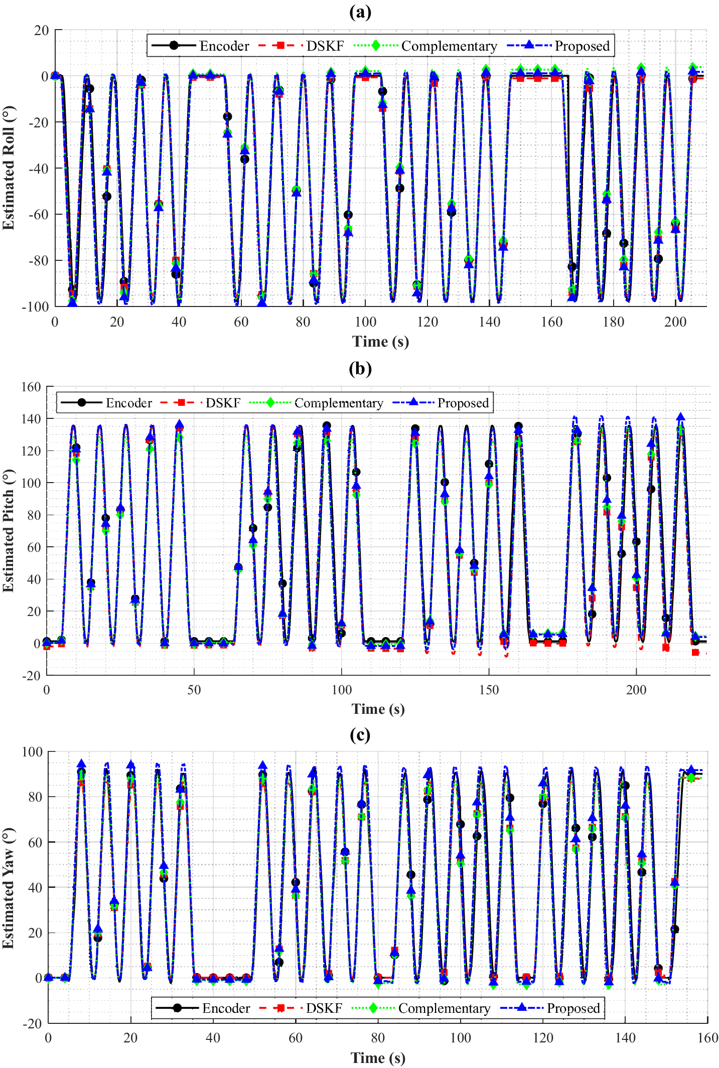
Figure 6. Sample results of orientation estimation for (a) Roll, (b) Pitch, and (c) Yaw trials on a SCORBOT ER-9 Pro robot, comparing the estimates of a double-stage Kalman filter, a complementary filter, and our proposed approach against the robot’s encoder reference measurements.
Table 1. Error analysis of sensor fusion methods: double-stage Kalman, complementary, and proposed filters Across roll, pitch, and yaw orientations
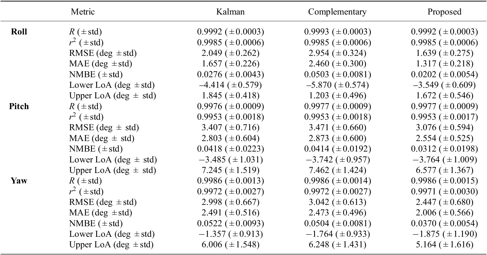
All methods demonstrated very high correlation coefficients ( $ R>0.997 $
) and coefficients of determination (
$ R>0.997 $
) and coefficients of determination ( $ {r}^2>0.995 $
) across all orientations, indicating strong linear relationships and predictive accuracy with the reference data. However, our proposed magnetometer-free method outperformed the other methods in terms of RMSE and MAE, especially in the yaw orientation. This suggests that, in a controlled environment, it provides better accuracy in estimating true values. Additionally, the proposed method exhibited the lowest NMBE across all orientations, indicating less measurement bias relative to the reference. The LoA analysis also highlighted the superior performance of the proposed method. It showed narrower ranges between the lower and upper LoAs, particularly in the yaw orientation, which suggests better agreement with the reference measurements.
$ {r}^2>0.995 $
) across all orientations, indicating strong linear relationships and predictive accuracy with the reference data. However, our proposed magnetometer-free method outperformed the other methods in terms of RMSE and MAE, especially in the yaw orientation. This suggests that, in a controlled environment, it provides better accuracy in estimating true values. Additionally, the proposed method exhibited the lowest NMBE across all orientations, indicating less measurement bias relative to the reference. The LoA analysis also highlighted the superior performance of the proposed method. It showed narrower ranges between the lower and upper LoAs, particularly in the yaw orientation, which suggests better agreement with the reference measurements.
3.2. Validity study results
Figures 7–
9 summarize the results of the data analysis phase comparing IMU-derived measurements to the VICON PiG model. All IMU traces presented in these figures were processed using the proposed approach. The std metrics reported in these figures reflect the variability between subjects and repetitions during the experimental trials. Specifically, it quantifies the differences in joint angle measurements across the volunteers performing ten repetitions of upper limb movements. In the figures, the notation $ {t}^{\ast } $
refers to the critical t-value, which identifies statistically significant differences between the IMU-based and reference VICON systems.
$ {t}^{\ast } $
refers to the critical t-value, which identifies statistically significant differences between the IMU-based and reference VICON systems.
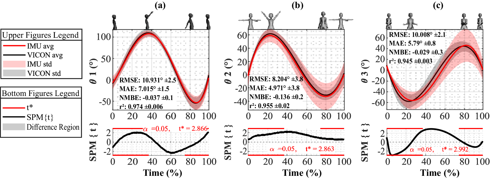
Figure 7. Comparative evaluation of IMU- and OMC-based systems for (a) shoulder flexion-extension $ {\theta}_1 $
, (b) shoulder adduction-abduction
$ {\theta}_1 $
, (b) shoulder adduction-abduction $ {\theta}_2 $
, and (c) shoulder internal-external rotation
$ {\theta}_2 $
, and (c) shoulder internal-external rotation $ {\theta}_3 $
DoF with SPM Analysis.
$ {\theta}_3 $
DoF with SPM Analysis.
The RMSE across all joints varied from 5.352° for wrist adduction-abduction to 12.075° for elbow pronation-supination. The MAE ranged from 3.688° for wrist adduction-abduction to 7.501° for elbow flexion-extension. The NMBE showed a minimal value of −0.839 in wrist flexion-extension, indicating potential underestimation, to a maximum of 0.143 in elbow flexion-extension, suggesting slight overestimation. These error metrics fall within 3–12.4% of the ROM (Namdari et al., Reference Namdari, Yagnik, Ebaugh, Nagda, Ramsey, Williams and Mehta2012; Raiss et al., Reference Raiss, Rettig, Wolf, Loew and Kasten2007) of the studied joints. The $ {r}^2 $
values, reflecting the correlation between the IMU and VICON data, were strongly positive, ranging from 0.890 in wrist adduction-abduction to 0.974 in shoulder flexion-extension.
$ {r}^2 $
values, reflecting the correlation between the IMU and VICON data, were strongly positive, ranging from 0.890 in wrist adduction-abduction to 0.974 in shoulder flexion-extension.
In shoulder joint motion monitoring, the comparative evaluation of IMU- and OMC-based systems across various DoF using SPM analysis is depicted in Figure 7. The analysis shows no significant differences in shoulder DoF $ {\theta}_1 $
,
$ {\theta}_1 $
, $ {\theta}_2 $
, and
$ {\theta}_2 $
, and $ {\theta}_3 $
between the IMU-based and the reference Vicon OMC system across all trials. In elbow joint motion monitoring, Figure 8 shows that there were no significant differences observed in elbow
$ {\theta}_3 $
between the IMU-based and the reference Vicon OMC system across all trials. In elbow joint motion monitoring, Figure 8 shows that there were no significant differences observed in elbow $ {\theta}_4 $
DoF during flexion-extension trials. However, significant differences were found in forearm
$ {\theta}_4 $
DoF during flexion-extension trials. However, significant differences were found in forearm $ {\theta}_5 $
DoF during pronation-supination trials between 44 and 59% of the motion cycles. For the wrist joint motion monitoring, Figure 9 shows that significant differences in
$ {\theta}_5 $
DoF during pronation-supination trials between 44 and 59% of the motion cycles. For the wrist joint motion monitoring, Figure 9 shows that significant differences in $ {\theta}_6 $
DoF were observed between 15 and 33% during flexion-extension, and
$ {\theta}_6 $
DoF were observed between 15 and 33% during flexion-extension, and $ {\theta}_7 $
DoF between 5 and 6.5% and 44 and 57% during adduction-abduction motion cycles.
$ {\theta}_7 $
DoF between 5 and 6.5% and 44 and 57% during adduction-abduction motion cycles.
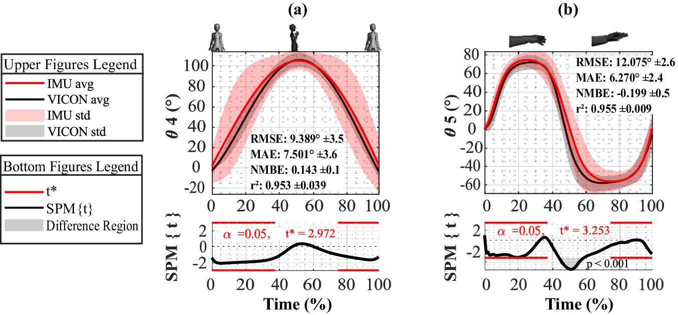
Figure 8. Comparative evaluation of IMU- and OMC-based systems for (a) elbow flexion-extension $ {\theta}_4 $
, and (b) forearm pronation-supination
$ {\theta}_4 $
, and (b) forearm pronation-supination $ {\theta}_5 $
DoF with SPM Analysis.
$ {\theta}_5 $
DoF with SPM Analysis.
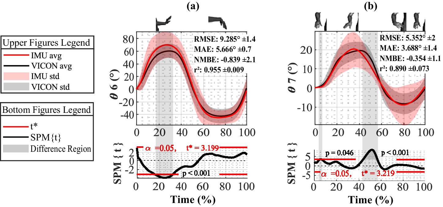
Figure 9. Comparative evaluation of IMU- and OMC-based systems for (a) wrist flexion-extension $ {\theta}_6 $
, and (b) wrist adduction-abduction
$ {\theta}_6 $
, and (b) wrist adduction-abduction $ {\theta}_7 $
DoF with SPM Analysis.
$ {\theta}_7 $
DoF with SPM Analysis.
4. Discussion
In this study, we proposed a novel magnetometer-free approach integrating the refined KF to correct orientation estimation. This approach aligns with clinical biomechanical practices prioritizing relative segment angles (e.g., arm elevation) over absolute heading (Cutti et al., Reference Cutti, Giovanardi, Rocchi, Davalli and Sacchetti2007). While pure yaw about the global vertical axis remains unobservable without magnetometers, studies confirm inclination-based metrics quantify functional ranges (e.g., shoulder abduction) with errors $ {5}^{\circ } $
(Picerno et al., Reference Picerno, Cereatti and Cappozzo2008). The method’s trade-off between sensor limitations and anatomical realities has been validated in applications ranging from stroke rehabilitation to athletic training, demonstrating its effectiveness for upper limb motions characterized by inclination-linked coupled kinematics rather than isolated yaw (Zhou et al., Reference Zhou, Hu and Tao2006).
$ {5}^{\circ } $
(Picerno et al., Reference Picerno, Cereatti and Cappozzo2008). The method’s trade-off between sensor limitations and anatomical realities has been validated in applications ranging from stroke rehabilitation to athletic training, demonstrating its effectiveness for upper limb motions characterized by inclination-linked coupled kinematics rather than isolated yaw (Zhou et al., Reference Zhou, Hu and Tao2006).
While extended Kalman filter (EKF) algorithms are typically preferred for human motion estimation due to their ability to handle nonlinear dynamics (Sabatini, Reference Sabatini2011), our approach employs a standard KF through careful system design. Nonlinear accelerometer-derived orientation angles ( $ {\phi}_a,{\theta}_a,{\psi}_a $
) are precomputed and treated as direct linear measurements within the filter, eliminating the need for EKF-based Jacobian linearization. The measurement matrix
$ {\phi}_a,{\theta}_a,{\psi}_a $
) are precomputed and treated as direct linear measurements within the filter, eliminating the need for EKF-based Jacobian linearization. The measurement matrix $ \mathbf{H} $
directly maps the state vector (containing orientation angles and gyroscope biases) to these preprocessed measurements, as validated in lightweight inertial fusion frameworks (Valenti et al., Reference Valenti, Dryanovski and Xiao2016). The gyroscope-driven prediction step utilizes a first-order kinematic model, which is valid for small
$ \mathbf{H} $
directly maps the state vector (containing orientation angles and gyroscope biases) to these preprocessed measurements, as validated in lightweight inertial fusion frameworks (Valenti et al., Reference Valenti, Dryanovski and Xiao2016). The gyroscope-driven prediction step utilizes a first-order kinematic model, which is valid for small $ \Delta t $
by avoiding nonlinear error growth (Luinge and Veltink, Reference Luinge and Veltink2005). This design reduces computational complexity to
$ \Delta t $
by avoiding nonlinear error growth (Luinge and Veltink, Reference Luinge and Veltink2005). This design reduces computational complexity to $ \mathcal{O}\left({n}^3\right) $
compared to EKF’s
$ \mathcal{O}\left({n}^3\right) $
compared to EKF’s $ \mathcal{O}\left({n}^3\right) $
plus Jacobian calculations, a critical advantage for real-time wearable IMU systems with limited processing resources (Särkkä, Reference Särkkä2013). By decoupling nonlinear operations from the filtering process and including linearized state transitions, our approach ensures sensor orientation estimation while prioritizing computational efficiency.
$ \mathcal{O}\left({n}^3\right) $
plus Jacobian calculations, a critical advantage for real-time wearable IMU systems with limited processing resources (Särkkä, Reference Särkkä2013). By decoupling nonlinear operations from the filtering process and including linearized state transitions, our approach ensures sensor orientation estimation while prioritizing computational efficiency.
In controlled robotic movements, the proposed magnetometer-free orientation estimation approach showed a superior performance, particularly in yaw estimation. This can be attributed to its combination of gyroscope and accelerometer data fusion within a KF framework, along with its direct alignment of the sensor frame with the global frame using accelerometer-derived angles. The proposed method includes the strengths of the gyroscope at capturing short-term dynamic changes in orientation and accelerometer at capturing long-term dynamic changes in orientation (Chen and Rong, Reference Chen and Rong2023; Trinh et al., Reference Trinh, Le, Tran, Cortes, Dario, Hoang, Voand Trong and Tran2020). By fusing these measurements, the algorithm compensates for the inherent limitations of each sensor, such as drift in gyroscope readings and noise in accelerometer data.
The traditional methods, however, rely on magnetometers for yaw correction, making them susceptible to magnetic disturbances (Chen and Rong, Reference Chen and Rong2023). The proposed method’s independence from magnetometer data contribute to more accurate yaw estimates, as evidenced by the lower RMSE, MAE, and NMBE values. This robustness against disturbances makes it suitable for diverse environments, including industrial applications. In addition, in real environments such as human motion, the variability in error metrics for the joints, observed across different movements, was noted to be within 3–12.4% of the joints’ ROM. This variability falls within acceptable limits for various motion capture technologies (Morrow et al., Reference Morrow, Lowndes, Fortune, Kaufman and Hallbeck2017; Schiefer et al., Reference Schiefer, Ellegast, Hermanns, Kraus, Ochsmann, Larue and Plamondon2014; Song et al., Reference Song, Hullfish, Silva, Silbernagel and Baxter2023), though it is unsuitable for applications requiring high precision (Berner et al., Reference Berner, Cockcroft and Louw2020; Nakano et al., Reference Nakano, Sakura, Ueda, Omura, Kimura, Iino, Fukashiro and Yoshioka2020). Additionally, the $ {r}^2 $
values ranged from
$ {r}^2 $
values ranged from $ 0.890 $
to
$ 0.890 $
to $ 0.974 $
, indicating a strong positive correlation and highlighting a high degree of correlation between IMU and VICON data.
$ 0.974 $
, indicating a strong positive correlation and highlighting a high degree of correlation between IMU and VICON data.
The variability in IMU-based system measurements is further demonstrated by the SPM analysis where motion cycle intervals with significant differences are identified. Namely, a significant difference was identified between IMU-based and OMC for the elbow joints motion cycles between 44 and 59% in $ {\theta}_5 $
of the cycles of forearm pronation-supination, corresponding to the return to the neutral position in the pronation phase.
$ {\theta}_5 $
of the cycles of forearm pronation-supination, corresponding to the return to the neutral position in the pronation phase.
Similarly, a significant difference between the two technologies was identified for the wrist joint. This difference is specifically in the wrist joints between 15 and 33% of wrist flexion-extension cycle $ {\theta}_6 $
, corresponding to the maximal flexion.
$ {\theta}_6 $
, corresponding to the maximal flexion.
A significant difference was also identified for the wrist joint in $ {\theta}_7 $
, where the IMU-based system underestimated the joint angle value between 5 and 6.5% of the motion cycle, corresponding to the beginning of the abduction phase, and between 44 and 57% of the motion cycle, corresponding to the end of the abduction phase. This could be related to the inherent nature of IMU as a similar observation has been done by Mittag et al., Reference Mittag, Leiss, Lorenz and Seel2020, who reported that IMU may not always capture the full range of wrist abduction, suggesting underestimation in some cases.
$ {\theta}_7 $
, where the IMU-based system underestimated the joint angle value between 5 and 6.5% of the motion cycle, corresponding to the beginning of the abduction phase, and between 44 and 57% of the motion cycle, corresponding to the end of the abduction phase. This could be related to the inherent nature of IMU as a similar observation has been done by Mittag et al., Reference Mittag, Leiss, Lorenz and Seel2020, who reported that IMU may not always capture the full range of wrist abduction, suggesting underestimation in some cases.
The variations observed among subjects in the precision of the joint measurements using the IMU-based system may be attributed to intersubject variations in sensor placement and movement-induced artifacts stemming from the sensor attachment methodology, as previously established in the literature (Wang et al., Reference Wang, Civillico, Niswander and Kontson2022).
Furthermore, it is noteworthy to mention that the precision of measurements obtained using IMU technology may decrease as the movement speed increases (Cooper et al., Reference Cooper, Sheret, McMillian, Siliverdis, Sha, Hodgins, Kenney and Howard2009). It is important to note that variations between the joint angles obtained using IMU-based and OMC technology are an inherent result of the different definitions of the segment axes and the distinct effects of soft tissue artifacts on the measurements (Cutti et al., Reference Cutti, Giovanardi, Rocchi, Davalli and Sacchetti2007).
While OMC systems have been established to provide reliable ground truth, it is important to acknowledge that, like all noninvasive techniques, OMC systems are subject to soft tissue artifact effects. According to Morrow et al. (Reference Morrow, Kaufman and An2011), the precision of a standard OMC system is within 3° of angular accuracy for human kinematics.
5. Conclusion
This study has addressed the critical challenges in sensor fusion for wearable IMU by proposing a magnetometer-free KF approach for robust and accurate orientation estimation. Traditional IMU-based systems, which often rely on magnetometers, face significant limitations due to magnetic interference and the need for extensive calibration processes. By eliminating the dependency on magnetometers, our approach enhances the versatility and reliability of IMU systems in diverse environments.
The proposed method effectively integrates gyroscope and accelerometer data using a refined KF, aligning the sensor frame with the Earth’s frame. This approach demonstrated superior performance across multiple metrics. In controlled robotic movements, the novel algorithm achieved an RMSE of 2.447° and MAE of 2.006° for yaw orientation, outperforming established techniques. The proposed method also showed the lowest NMBE across all orientations, indicating minimal measurement bias relative to reference data. The LoA analysis confirmed the results of the proposed method, with narrower ranges between the lower and upper LoAs, especially in yaw orientation, suggesting better agreement with reference measurements.
In real-world applications, such as upper limb motion monitoring, the variability in error metrics for joint measurements was within 3–12.4% of the joints’ ROM. This variability is acceptable for many motion capture technologies, although further refinement is needed for high-precision applications. The method demonstrated low error metrics and a strong positive correlation with VICON data, highlighting the high degree of agreement between the IMU-based and the OMC systems.
The SPM analysis further revealed motion cycle intervals with significant differences between the IMU-based system and the OMC system. Short but significant intervals of differences in joint motion cycles were observed in the elbows and wrists. These discrepancies are likely related to the inherent nature of IMU, as they sometimes underestimate or overestimate joint angles, particularly in complex movements.
The proposed magnetometer-free KF approach offers a promising alternative for accurate and reliable orientation estimation in environments with magnetic distortions. By minimizing manual calibration requirements and incorporating detailed algorithmic refinements, this method has significant potential for improving sensor fusion technology in dynamic and complex settings. Future research will focus on optimizing the algorithm for real-time applications on devices with limited processing power and enhancing the method’s accuracy and stability for diverse motion dynamics.
Data availability statement
The datasets collected and analyzed during this study are not publicly available due to confidentiality and ethical restrictions related to human participant data.
Authorship contribution
Conceptualization: S.B. (Souha Baklouti), T.R., and A.C.; Data collection: S.B. (Souha Baklouti); Data curation: S.B. (Souha Baklouti); Formal analysis: S.B. (Souha Baklouti); Funding acquisition: A.S.; Investigation: S.B. (Souha Baklouti) and T.R.; Methodology: S.B. (Souha Baklouti), S.B. (Sami Bennour), T.R., and A.C.; Project administration: S.B. (Sami Bennour) and A.S.; Resources: A.S.; Software development: S.B. (Souha Baklouti); Supervision: S.B. (Sami Bennour) and A.S.; Validation: S.B. (Souha Baklouti), S.B. (Sami Bennour), T.R., and A.C.; Writing–original draft preparation: S.B. (Souha Baklouti); Writing–review and editing: T.R., A.C., S.B. (Sami Bennour), and A.S. All authors have read and agreed to the published version of the manuscript. All authors approved the final submitted draft.
Funding statement
This project is carried out under the MOBIDOC scheme, funded by The Ministry of Higher Education and Scientific Research through the PromEssE project and managed by the ANPR (The National Agency for the advancement of scientific research).
Competing interests
The authors declare no competing interests exist.
Ethical standard
The study was conducted in accordance with the Declaration of Helsinki and approved by the Ethics Committee for Life and Health Sciences Research of the Higher Institute of Biotechnology of Monastir (ISBM) (protocol code CERSVS/ISBM 018/2023).


 Open access