

1. INTRODUCTION
Englacial channels deliver surface meltwater to the interior and base of ice masses (Fountain and Walder, Reference Fountain and Walder1998; Irvine-Fynn and others, Reference Irvine-Fynn, Hodson, Moorman, Vatne and Hubbard2011). This delivery influences glacier mass balance as a result of its close association with ice dynamics (e.g. Iken and Bindschadler, Reference Iken and Bindschadler1986; Zwally and others, Reference Zwally, Abdalati, Herring, K L, Saba and Steffen2002; Mair, Reference Mair2005; Schoof, Reference Schoof2010), water storage (Jansson and others, Reference Jansson, Hock and Schneider2003; Lingle and Fatland, Reference Lingle and Fatland2003) and thermal energy transfer within the glacier system (Phillips and others, Reference Phillips, Rajaram and Steffen2010; Mankoff and Tulaczyk, Reference Mankoff and Tulaczyk2017). Englacial drainage networks have been identified and described in temperate (e.g. Harper and Humphrey, Reference Harper and Humphrey1995; Piccini and others, Reference Piccini, Romeo and Badino2002; Gulley, Reference Gulley2009) and polythermal glaciers (e.g. Pulina, Reference Pulina1984; Holmlund, Reference Holmlund1988; Moorman and Michel, Reference Moorman and Michel2000; Gulley and others, Reference Gulley, Benn, Müller and Luckman2009a), with more recent observations highlighting the existence of englacial conduits in cold ice margins (Vatne, Reference Vatne2001; Benn and others, Reference Benn, Gulley, Luckman, Adamek and Glowacki2009; Gulley and others, Reference Gulley, Benn, Müller and Luckman2009a; Bælum and Benn, Reference Bælum and Benn2011; Naegeli and others, Reference Naegeli, Lovell, Zemp and Benn2014) and ice-sheet settings (Catania and others, Reference Catania, Neumann and Price2008; Das and others, Reference Das2008). However, these conduits are difficult to access directly and, consequently, a process-level understanding of their geometry, formation and evolution remains poorly constrained (Vatne and Irvine-Fynn, Reference Vatne and Irvine-Fynn2016).
To date, knowledge of englacial hydrological systems has been inferred from borehole observations (Harper and Humphrey, Reference Harper and Humphrey1995; Fountain and others, Reference Fountain, Jacobel, Schlichting and Jansson2005), dye-tracing experiments (Willis and others, Reference Willis, Sharp and Richards1990; Nienow and others, Reference Nienow, Sharp and Willis1998; Bingham and others, Reference Bingham, Nienow, Sharp and Boon2005; Irvine-Fynn and others, Reference Irvine-Fynn, Hodson, Kohler, Porter and Vatne2005) and geophysical surveys (Moorman and Michel, Reference Moorman and Michel2000; Stuart, Reference Stuart2003; Catania and others, Reference Catania, Neumann and Price2008) or directly assessed with speleological explorations using traditional cave surveying techniques (Pulina, Reference Pulina1984; Vatne, Reference Vatne2001; Vatne and Refsnes, Reference Vatne and Refsnes2003; Gulley and others, Reference Gulley, Benn, Müller and Luckman2009a,Reference Gulley, Benn, Screaton and Martinb). Although the last provides the only direct observations of the interior of englacial channels, the spatial resolution of these surveys are limited, with dimensional measurements and sketches of cross-section morphology being carried out at changes in channel orientation and inclination (Warild, Reference Warild2007). In englacial channels, the intervals between such changes are typically on the order of several to tens of metres, meaning that such surveys provide sparse coverage over mapped reaches of up to hundreds of metres and, thus, provide little morphological detail. Given that channel morphology can alter over much smaller spatial scales, due to complex feedback mechanisms between morphology and flow dynamics, finer resolution surveys are required for enhancing understanding of englacial channel geometry and its temporal evolution across daily to decadal timescales.
Recent technological development, in the form of terrestrial laser scanning (TLS), provides an opportunity to improve upon these manual measurements of englacial morphology. In geomorphological and industrial settings, TLS is already an established tool for mapping of rock and ice-coated caves (Buchroithner and others, Reference Buchroithner, Gaisecker, Gaisecker and Österreich2009; Cosso and others, Reference Cosso, Ferrando and Orlando2014; Gallay and others, Reference Gallay, Kaňuk, Hochmuth, Meneely and Hofierka2015; Idrees and Pradhan, Reference Idrees and Pradhan2016) and artificial tunnels (Li and others, Reference Li, Youchan and Xianjun2012). TLS enables rapid acquisition (minutes to hours) of high accuracy datasets at millimetre-scale spatial resolution, allowing for detailed retrospective measurements of target features to be made at fine spatial intervals (Lichti and others, Reference Lichti, Gordon and Stewart2002; Pfiefer and Briese, Reference Pfiefer and Briese2007). Within cryospheric research, TLS has been successfully used to recreate 3-D snow and ice surfaces, allowing determination of snow depth distributions (Jörg and others, Reference Jörg, Fromm, Sailer and Schaffhauser2006; Kaasalainen and others, Reference Kaasalainen, Kaartinen and Kukko2008; Osterhuber and others, Reference Osterhuber, Howle and Bawden2008; Prokop, Reference Prokop2008), glacier surface roughness (Smith and others, Reference Smith2016), surface ablation (Gabbud and others, Reference Gabbud, Micheletti and Lane2015) and mass balance (Fischer and others, Reference Fischer, Huss, Kummert and Hoelzle2016). Therefore, TLS could provide an innovative alternative to current glacio-speleological methods of cartography and morphological analysis. To our knowledge, a detailed morphological assessment of an englacial channel using TLS has yet to be undertaken, largely as a result of the challenges presented by the optical and physical properties of ice (Lichti and others, Reference Lichti, Gordon and Stewart2002) and the practicalities of using older TLS instruments in these more rugged environments.
Here, we describe the novel use of TLS technology to reconstruct the internal geometry of an englacial channel in the High Arctic glacier, Austre Brøggerbreen, detailing the practical survey methods and data processing techniques used to recreate and map conduit morphology. The results are used to evaluate the potential of TLS for mapping of ice-walled channels, as an improvement on traditional manual surveying for morphological analyses.
2. FIELD SITE AND DATA ACQUISITION
2.1. Field site
Austre Brøggerbreen is a 5 km long, predominantly cold-based, valley glacier located on the Brøggerhalvoya Peninsula, Svalbard (79° 55′ N, 11° 46′ E; Fig. 1). The glacier extends from ~50 to 600 m a.s.l., covering an area of ~9.4 km2 with an ice thickness of <100 m, and comprising six flow units that feed into a relatively short tongue (Bruland and Hagen, Reference Bruland and Hagen2002; Porter and others, Reference Porter, Vatne, Ng and Irvine-Fynn2010; Jennings and others, Reference Jennings, Hambrey, Glasser, James and Hubbard2015). Low ice surface velocities of <3 m a−1 (Hagen and others, Reference Hagen, LiestøL, Erik and Jørgensen1993), together with recent downwasting and recession (Barrand and others, Reference Barrand, James and Murray2010), have led to the transition of the glacier from a polythermal regime to a cold-based one (cf. Hagen and Sætrang, Reference Hagen and Sætrang1991; Björnsson and others, Reference Björnsson1996; Nowak and Hodson, Reference Nowak and Hodson2014). This change in thermal structure has facilitated the development of an extensive and stable supraglacial drainage network, with several deeply incised surface channels feeding into perennial moulins. Formation of englacial channels through cut-and-closure mechanisms form a substantial part of Austre Brøggerbreen's hydrological system (Vatne, Reference Vatne2001; Stuart, Reference Stuart2003; Vatne and Refsnes, Reference Vatne and Refsnes2003; Vatne and Irvine-Fynn, Reference Vatne and Irvine-Fynn2016), which drains through a main portal at the eastern glacier margin (Porter and others, Reference Porter, Vatne, Ng and Irvine-Fynn2010).
Map of Austre Brøggerbreen. The moulin investigated with TLS is located ~1200 m from the glacier terminus. Numbered flow unit boundaries as identified by Jennings and others (Reference Jennings, Hambrey, Glasser, James and Hubbard2015), and the portal through which englacial drainage exits the glacier, are depicted. The location of Austre Brøggerbreen within Svalbard is highlighted on the inset map.
Since 1998, a persistent englacial conduit on the easternmost flow unit has been repeatedly mapped using traditional cave surveying techniques, in order to characterise its morphological evolution. Over time, the channel has changed from an incised, down-glacier sloping supraglacial stream with many knickpoints, to a vertical moulin descending to a depth of ~50 m below the ice surface, which then feeds a low gradient, meandering englacial system (Myreng, Reference Myreng2015; Vatne and Irvine-Fynn, Reference Vatne and Irvine-Fynn2016).
2.2. Fundamentals of TLS
Numerous detailed reviews of TLS are available (e.g. Heritage and Large, Reference Heritage and Large2009; Vosselman and Maas, Reference Vosselman and Maas2010; Lemmens, Reference Lemmens2011), and we provide a brief overview of the key terms used herein. TLS is an active remote-sensing technique that allows reconstruction of the surface of a feature in 3-D, using the emission and detection of a laser beam from a static point on the ground to calculate the distance between the object and the sensor (Pfiefer and Briese, Reference Pfiefer and Briese2007; Petrie and Toth, Reference Petrie, Toth, Shan and Toth2008; Heritage and Large, Reference Heritage and Large2009). TLS typically uses an infrared wavelength laser beam that can be emitted either continuously (phase-shift method), or as a pulse (time-of-flight or pulse-based method (Petrie and Toth, Reference Petrie, Toth, Shan and Toth2008; Deems and others, Reference Deems, Painter and Finnegan2013)). Each laser beam return creates a 3-D point in relative space around the instrument, producing a point cloud that represents the surface of a scanned object. The density and spacing of points is theoretically dependent on scan resolution, with optimal resolution being a trade-off between the highest number of points required for the project purpose and the scan duration. Resolution is an instrument parameter expressed as a fraction, with higher resolutions requiring greater scanning time. In the case of the FARO® Focus3D X 330 scanner used herein, a maximum resolution of 1/1 takes 30.34 min to complete (LaserscanningEurope, 2015); typical scans using this instrument are carried out at 1/5 to 1/4 resolution, taking 5–10 min.
2.3. TLS field surveying
TLS of the glacier surface surrounding the moulin entrance, the moulin shaft and englacial conduit were carried out over 4 d in March 2016, when the channel was hydrologically inactive. Scans were conducted using a FARO® Focus3D X 330 phase-shift scanner (360° horizontal field-of-view; 300° vertical field-of-view) with a shortwave infrared wavelength of 1550 nm (FARO Technologies Inc., 2013), mounted on a Gitzo™ Mountaineer carbon fibre tripod using a heavy duty 3/8″ camera fast-release mount. An insulation cover for the scanner head was fashioned from 0.8 cm thick foam, with insertion of exothermic hand warmers at the base of the cover to prevent the scanner from becoming inoperable in sub-zero temperatures (Fig. 2). Three scans at 1/4 resolution (point spacing of 6.14 mm at a 10 m range (LaserscanningEurope, 2015)) were completed around the moulin circumference at the glacier surface, using the in-built GPS scanner function. In the absence of GPS signal below the ice, these surface scans provided georeferenced data from which the conduit point clouds were converted to absolute coordinates. Consequently, a higher resolution was used for the surface scans than that used for the conduit. Four spherical fishing buoys (radius: 10.4 cm) mounted on short drainpipe sections were used as targets, with their positions recorded using a portable Trimble Pathfinder® Pro XR differential GPS (dGPS), which were used to further correct surface scans to horizontal and vertical precisions of 0.61 and 1.68 m, respectively. Surface scans were conducted as close to the moulin entrance as safely possible, enabling scanning of the uppermost 3 m of the moulin shaft, relative to which the below-surface scans were co-registered.
The scanner in situ (A) demonstrating the insulation cover and placement of the exothermic hand warmers. Scalloping can be seen on the wall to the left of the scanner. Placement of the checkerboard targets within the conduit (B) on the wall and floor of the channel, with spacing of the latter at ⩾1 m. Longitudinal grooves are visible on the right wall. Both images show the snow, hoar frost, clean glacier ice and sediment-rich ice surfaces present within the channel.
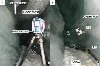
Mapping of the uppermost englacial conduit reach was achieved by conducting 25 laser scans, extending from the base of the moulin to a horizontal distance along the thalweg of 122 m. Scans were carried out at 1/5 resolution (point spacing of 7.67 mm at a 10 m range (LaserscanningEurope, 2015)) and were acquired at horizontal intervals of between 1.75 and 9 m, with the TLS instrument mounted ~1.5 m above the cave floor. This variability in scan spacing depended on the channel sinuosity, with positioning to achieve maximum wall coverage using the minimum number of scans. Similarly, positioning of the scanner within the channel cross-section depended on the conduit morphology, in order to minimise beam shadowing. Double-sided ‘A4’ (29.7 × 21 cm) planar checkerboard targets were attached to ice screws using crocodile clips and inserted at varying heights perpendicular to the conduit walls, with smaller ‘A5’ (21 × 14.8 cm) targets of the same design placed at shorter spatial intervals at floor level (Fig. 2). These targets were positioned to ensure scan coverage of a minimum of three registration tie-points through forward planning of the subsequent two scanner locations, allowing for the likelihood of targets being knocked within the confined space. At each scan location, in situ air temperature and relative humidity were recorded using a Kestrel® 3000 pocket weather meter. Scan validation was accomplished through manual surveying of a 58 m conduit section, using a Leica Disto™ laser range finder and compass, to a survey grade 2/3 C (BCRA, 2017).
2.4. Point cloud processing
The resulting 3-D point clouds were post-processed using FARO® SCENE (FARO Technologies Ltd, 2016) and Rhino3D® (Robert McNeel & Associates, 2017) software. Surface scans were georeferenced and corrected using the dGPS coordinates of the spherical targets to enable below-surface scan registration in absolute coordinates. The conduit scans were relatively positioned, using the common moulin shaft sides and cornices captured in both the surface and below-surface scans. The depth and angular positioning of the conduit scans was corroborated by knowledge of the unloaded abseil rope length, and through examination of 360° photography of the moulin base (Digital Explorer, 2016). Manual registration of conduit scans enabled greater operator control, due to the lack of distinguishable features within the channel from which automatic algorithms could match overlapping areas. Registration of each scan to the preceding scan was conducted to within 6.8 mm positional accuracy, using between three and eight tie-points to achieve the lowest orthogonal mismatches possible.
Using FARO® SCENE, filtering of individual point clouds to remove speckle and edge effect noise was carried out post-registration to allow for retention of tie-points, with application of ‘distance-based’ and ‘stray’ filters removing 14.75 ± 5% of scan points. Filtering thresholds were established to remove visible noise, ensuring minimal compromising of the dataset, which would otherwise prevent mapping of cross-section morphology. Reflectivity percentages were calculated from the dimensionless raw reflectivity values of each point, in order to create a meaningful measure of reflectance from which to interpret the point cloud. Laser beam returns, defined as light reflected back to the scanner to create a point, are expressed as a percentage of the theoretical maximum number of laser returns.
2.5. Extraction of 2-D channel geometry
Digitisation of the filtered point clouds to extract 2-D geometry was completed using Rhino 3D® software with the Veesus Arena4D point cloud plugin, using point cloud slicing in the horizontal and vertical planes. Slicing widths were determined through visual inspection of the point cloud slices, to provide the best representation of a discrete profile while accounting for data losses. Linear representations of these point cloud slices were created by manually drawing lines of best fit through the centre of the points. Manual digitisation allowed for user control, accounting for areas of data exclusion and preventing incorrect mapping of edge effects. The channel planform was digitised at 1 m above the channel floor throughout the conduit. The moulin base was digitised 3 m above the floor, in order to exclude the snow and ice-block infill at the bottom of the shaft. Cross-section geometries were extracted using a 0.2 m width slice at 1 m intervals from the conduit entrance.
3. RESULTS
3.1. Englacial channel morphology
Throughout the conduit, the channel walls comprised clean glacier ice, with evidence of scalloping, tensional veins and continuous sediment bands of reddish-brown and light-grey colour cutting across the walls. Although numerous, these bands did not account for a large surface area. Hoar frost covered the uppermost sections of the conduit wall and ceiling, and snow composed of visibly large, consolidated crystals formed a blocky false floor (Fig. 2). Snow on the order of metres to several tens of metres thick unevenly covered the base of the moulin.
The 25 point clouds comprise over 261 million individual points, from which channel morphology was extracted (Fig. 3). Figure 3A shows that the conduit leads south-west from the base of the moulin, at a depth of 48 m below the ice surface. The channel planform shows regular meanders, with a high sinuosity of 2.7 and a curvature radius of 4 m. Over the mapped reach of 122 m, the channel lowers by 5.65 m, with a step made up of ice breccia covered by winter snowfall observed at the channel entrance accounting for 4.93 m of this (Fig. 3B). From the base of this step, the remainder of the channel remains relatively flat, lowering by only 0.67 m over 116 m length.
(A): The channel planform, with the section used for cross-section analysis in (C) highlighted in black. The numbers correspond with those in (C) to denote cross-section locations; (B) the longitudinal profile – the dip at the base of the moulin shaft denotes the snow-covered moulin floor, with the rise in elevation to the top of the step; (C) channel cross-section morphology at 1 m intervals around the first meander bend blacked out in (A), progressing from left to right. The direction of flow is into the page, with the red dashed line providing a reference plane at 2 m above the floor. The teardrop shape with the presence of grooves and the tilt towards the inside bend can be seen. Discontinuous lines indicate areas without data, as a result of beam shadowing.
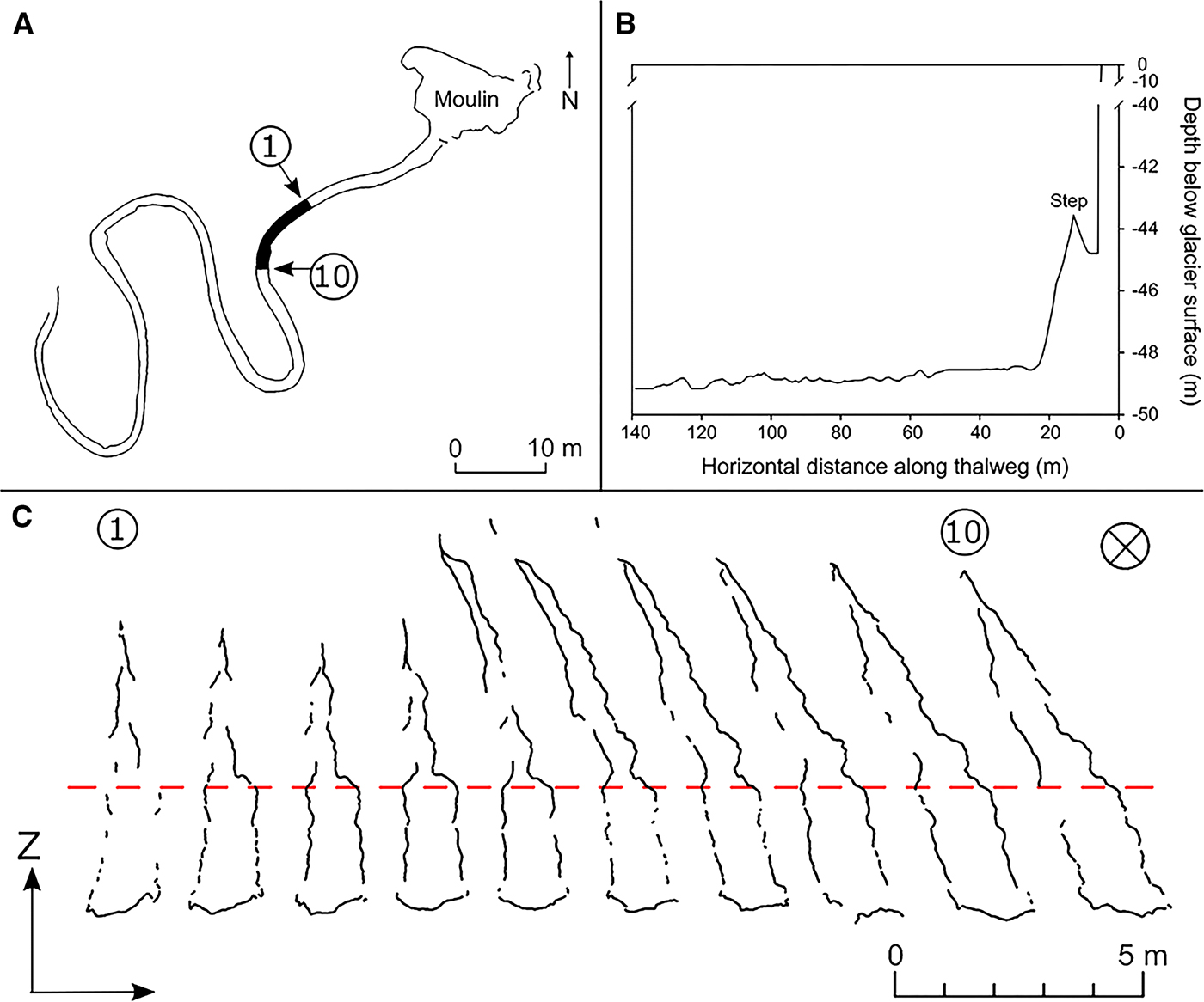
The conduit cross-section morphology is generally teardrop shaped, with tapering walls that meet between 5 and 12 m above the channel floor. Analysis of cross-section change with distance downstream demonstrates that the axis of the teardrop shape becomes increasingly tilted towards the inside bank around meander bend apexes, with a tilt of up to 25° being observed over a 10 m reach (Fig. 3C). Longitudinal grooves run the length of the conduit on either wall, with irregular groove spacing ranging between 0.94 and 2.05 m. The conduit width wall-to-wall is widest at the entrance to the channel (1.97 m), decreasing to <1 m downstream, with the narrowest section (0.68 m) located 6 m from the end of the mapped reach.
3.2. Conduit wall laser returns
Despite the point cloud successfully providing highly detailed 3-D visualisation of the conduit interior at a fine spatial resolution (Fig. 4), the overall laser returns were 38 ± 16%, indicating that nearly two-thirds of the emitted laser beams were not reflected back to the instrument. Several areas of each point cloud are devoid of data, most notably at regular vertical intervals along the channel wall and some sections of the conduit ceiling (Fig. 3C), resulting in ‘holey’ point clouds. The reflectivity percentage of the clean ice walls decreases significantly as the angle of incidence increases (r = −0.47, n = 50, P ⩽ 0.01): incidence angles of <30° exhibit a reflectivity of 31%, compared with 22–25% for angles >30°.
Three-dimensional point cloud visualisation of the moulin shaft and englacial conduit, showing perspective (A), plan (B) and side (C) views to demonstrate the success of the TLS reconstruction. For further visualisation of the TLS survey results in three-dimensions, the reader is directed to the following links for a fly-through video of the moulin and conduit (www.youtube.com/watch?v=o7uOGKb0kwc) and panoramic visualisation of the interior (www.derij.co.uk/images/panos/SV2016/SV2016.html).
Analysis of reflectivity data indicates the presence of four reflectively distinct zones within the conduit. These differences are manifested spatially as contrasts between the channel floor, roof, and walls, with respective reflectivity percentages of 34 ± 4%, 31 ± 5% and 24 ± 5%, with thin linear features of 46 ± 7% reflectivity cutting across the conduit walls (Fig. 5). These variations correspond with snow cover at the base of the channel, hoar frost crystals in the conduit ceiling and the clean ice walls with entrained sediment bands, as validated from colour photographs taken at each scanner location. Results of analysis of variance tests indicate a significant difference between each of these surfaces (P < 0.01). Numerous thin bands of high reflectivity (40 ± 4%) were identified on the scans that were not immediately visible in the optical imagery (Fig. 5B), but through image analysis were found to be associated with sediment inclusions that were not exposed at the ice-wall surface. Similar to ice, a positive relationship between incidence angles and snow reflectivity was found (r = 0.53, n = 50, P ⩽ 0.01).
Colour photograph (A) and greyscale visualisation of scan reflectivity values for the same view (B), demonstrating differences in laser beam return from varying materials. Visible sediment bands cutting across either conduit wall can be seen in both panels, with fine vertical stripes visible on the right wall of (B) showing the thinner sediment bands or fractures that are not exposed at the ice wall; hoar frost can be seen on the upper section of this wall. Wall targets (A4) and floor targets (A5) are visible in both image panels for scale. Additional scale visible just left-of-centre includes a person (panel A) and an ice axe (panel B).

3.3. Accuracy and precision
The registration accuracy has a maximum error of 6.8 mm, with a mean error of 3.3 mm, representing the std dev. of orthogonal registration mismatch between adjacent scans, expressed as cumulative distance offset in the X, Y and Z planes (FARO Technologies Inc., 2015). However, the unclosed traverse from the moulin base to the end of the scanned conduit prevents equal error distribution between scans. This yields a maximum combined absolute error of 73 mm by the end of the traverse, derived from the sum of orthogonal mismatches for the 25 scans.
In order to evaluate the accuracy at which the laser beam identifies the solid ice surface, variance of the point cloud data from a plane of best fit was quantified (linear least squares; n = 50). Although flat 0.05 m2 areas of the conduit wall devoid of sediment inclusions were selected for this analysis, it must be acknowledged that the ice surface is inevitably curved over an area containing sufficient points to enable plane fitting. This method yields an accuracy of ±6.54 mm for detection of the ice walls, compared with a mean error of ±2.19 mm for the solid surface of the checkerboard targets (comparable to the quoted manufacturer's accuracy of ±2 mm (FARO Technologies Inc., 2011)).
Despite the scatter of points around the plane of best fit being within 1 cm of the ice wall surface, the scans reveal numerous individual points located at apparently regular intervals beyond the channel wall (⩽0.61 m). These extraneous points are arranged as a series of linear features parallel to the channel walls, and correspond with the location of the ice screws holding the checkerboard targets in place (Fig. 6). These features are interpreted to be representative of ice fracturing, which occurred perpendicularly around the shaft of the screw during insertion (e.g. Hill, Reference Hill2006).
Plan view of the A4 checkerboard target and the points within the channel wall, interpreted as fracturing of the ice around the ice screw shaft during insertion. The dotted line denotes the ice wall surface. Points surrounding the target are the result of edge effect noise that is visible when presented in plan view.
Assessment of scan precision was achieved through quantification of linear offsets between areas of overlapping scans (n = 50). Planes of best fit were created for areas of point cloud overlap between adjacent scans, with measurement of each individual scan's point cloud deviation from this plane. This provided an overall scan precision of ±10 cm.
3.4. Influence of meteorological conditions
Within the conduit, air temperature varied between −1 and −4.9°C, typically being ~−3.5°C. Relative humidity was between 79 and 97%, compared with an average March atmospheric relative humidity of ~70% for the nearby settlement of Ny-Ålesund at 2 m above ground (Maturilli and others, Reference Maturilli, Herber and König-Langlo2013). The FARO® Focus3D X 330 provided consistent instrumental operation in temperatures as low as −5°C, providing that the scanner temperature remained above 3°C. Insulation of the scanner head maintained instrument temperatures of >17°C throughout the duration of surveying, with air temperature having a negligible effect. However, ceasing of instrument operation for 50 min resulted in a decrease in scanner temperature from 21 to 3°C, with recommencement leading to a temperature rise of 14°C in 20 min, as a result of the scanner generating heat when operating. Although correlations between meteorological conditions and laser beam returns show that higher returns are associated with colder temperatures and lower relative humidity (respectively, r = −0.47; r = 0.2, n = 17), these relationships are not significant (P > 0.05). However, wind chill at the glacier surface lowered air temperatures to −25°C, resulting in scanner shutdown. Cold operating temperatures also slowed the rate at which scan surveys could be conducted, as a result of the logistical impacts of undertaking fieldwork in low-temperature environments.
4. INTERPRETATION AND DISCUSSION
4.1. Channel morphology
The englacial channel's longitudinal profile and planform are consistent with the previous conduit survey conducted in 2014, which demonstrated regular meandering at a constant depth (Myreng, Reference Myreng2015). The development of the vertical moulin shaft and these meanders were first recorded in 2008 (Vatne and Irvine-Fynn, Reference Vatne and Irvine-Fynn2016), indicating that these features may be relatively stable in their general form over annual to inter-annual timescales. As changes in channel bed slope are one of the most efficient ways of dissipating energy (Knighton, Reference Knighton1998), the consistent conduit depth indicates that adequate energy dissipation is achieved by the existing channel morphology. This suggests that the vertical drop of water over the moulin edge acts to efficiently dissipate the majority of the stream's energy (Curran and Wohl, Reference Curran and Wohl2003).
The teardrop cross-section morphology denotes passage closure as a result of ice creep deformation, bringing the two walls into contact to form a sutured canyon indicative of the channel's cut-and-closure origin (Gulley and others, Reference Gulley, Benn, Müller and Luckman2009a). Furthermore, the longitudinal grooves are interpreted to represent fluctuations in, or modes of, meltwater discharge (Vatne and Irvine-Fynn, Reference Vatne and Irvine-Fynn2016), with lateral thermal expansion at times of high discharge and vertical channel incision under reduced flow conditions (Marston, Reference Marston1983).
4.2. Laser returns from clean ice
In the fully enclosed conduit environment, the low percentage of overall returns is likely explained by the properties of the scan surface or the environmental conditions (Smith, Reference Smith, Cook, Clarke and Nield2015). The majority of the scanned surface comprised clean ice, which has a high absorption coefficient in the infrared (~1.6 cm−1) with significant absorption bands around the 1550 nm wavelength of the scanner used herein (Hobbs, Reference Hobbs1974; Warren and Wiscombe, Reference Warren and Wiscombe1981; Warren, Reference Warren1982). The depth to which electromagnetic radiation can penetrate below the surface of a material is one of the primary variables controlling its reflectance (Picard and others, Reference Picard, Libois and Arnaud2016), meaning that clear ice effectively absorbs these wavelengths (Hobbs, Reference Hobbs1974; Lucey and Clark, Reference Lucey, Clark, Klinger, Benest, Dollfus and Smoluchowski1985). This causes photon extinction just below the ice surface, accounting for laser beam losses and low returns. Such losses using infrared wavelengths have also been reported on glacier surface ice, where clean ice exhibited a low percentage of returns and, consequently, sparse data coverage (Hopkinson, Reference Hopkinson2004). Furthermore, the low reflectivity of the smooth, shiny, ice surface at high incidence angles causes laser beam deflection away from the scanner (Jörg and others, Reference Jörg, Fromm, Sailer and Schaffhauser2006; Soudarissanane, Reference Soudarissanane2016), meaning that low amounts of radiation are reflected back to the instrument, resulting in reduced or no measurements (Heritage and Large, Reference Heritage and Large2009). Therefore, distance from the scanner becomes a major limiting factor in scanning oblique ice surfaces, as the incidence angle increases with distance (Soudarissanane and others, Reference Soudarissanane, Lindenbergh and Gorte2008; Heritage and Large, Reference Heritage and Large2009; Pejić, Reference Pejić2013).
The geometric properties of the conduit's ice wall can also influence the existence, location and intensity of a returned laser beam point (Lichti and others, Reference Lichti, Gordon and Stewart2002). The cross-section geometries show that the existence of a point is primarily dependent on the line-of-sight principle, with areas devoid of data coinciding with curved areas of the channel roof and the troughs of longitudinal grooves (Fig. 3C). This indicates laser beam obstruction, resulting in the creation of shadowed areas and, thus, determining the scan features that can be represented within the point cloud. Furthermore, the wall morphology underpins the intensity of the return, with ice surfaces perpendicular to the scanner providing the greatest intensities. This demonstrates that positioning of the scanner in relation to the conduit geometry determines the areas where beam reflectance will be maximised and, subsequently, point cloud density (Soudarissanane and others, Reference Soudarissanane, Lindenbergh, Menenti and Teunissen2011).
As the cool conditions within the englacial channel are considered favourable for laser scanning (Baltsavias, Reference Baltsavias1999), it would be expected that returns would be maximised in this environment. However, as Section 3.4 demonstrates no significant relationship between either air temperature or relative humidity and percentage returns, factors beyond the meteorological conditions reported here exert an influence on laser returns. This assertion is supported by the ability to achieve the instrument's reported accuracy of 2 mm on the target surfaces. Therefore, over these temperature and humidity ranges, the physical and optical properties of the conduit walls and glacier ice have a greater influence on the quality of laser returns in this environment.
4.3. Laser returns from snow, hoar frost and sediment
In the shortwave infrared, the laser returns from snow, hoar frost and sediment are significantly higher than that of the least reflective clean glacier ice herein, with reflectivity values at least 7% greater than the conduit walls. Although the spectral reflectance of snow and hoar frost is low in this wavelength (Foster and others, Reference Foster, Hall and Chang1987; ESA, 2014), their absorption coefficients are lower than that of ice, meaning that they are more reflective (Joseph, Reference Joseph2005), with the higher surface roughness of these materials further increasing their reflectivity (Choudhury and Chang, Reference Choudhury and Chang1981; Schaffhauser and others, Reference Schaffhauser2008). However, the greatest reflectivity is from the sediment bands, indicating the presence of high particle concentrations exposed at the wall surface and in the near-surface ice (Alfoldi, Reference Alfoldi, Johannsen and Sanders1982; Lucey and Clark, Reference Lucey, Clark, Klinger, Benest, Dollfus and Smoluchowski1985; Karabulut and Ceylan, Reference Karabulut and Ceylan2005).
As the scan data detected thinner, discrete sediment bands that were not exposed at the wall surface, this suggests that the laser is able to detect sediment located at depths greater than the ice absorption coefficient. This could be the result of the sediment mineral properties, as the constituent minerals of the red sandstone, limestone and quartz bedrock geology underlying the eastern parts of Austre Brøggerbreen (Nowak and Hodson, Reference Nowak and Hodson2014) have very high reflectance in the infrared, contributing to their detection within the ice substrate (Gibson, Reference Gibson2000; Choudhury and others, Reference Choudhury, Chakrabarti and Choudhury2009). Although the sediment type within such discrete bands cannot be confirmed, the colour of the exposed sediment accords with this bedrock geology. Conversely, this detection may be facilitated by the evidence of below-surface ice fracturing (Fig. 6), which suggests that the laser may either: (i) be reflected from sub-surface structural inhomogeneities, providing a return where homogeneous intact ice does not, and/or (ii) be able to exploit existing structural weaknesses when scanned at certain angles.
4.4. Data quality and methodological considerations
The accuracy assessment demonstrates that TLS can provide high-quality data, accurate at millimetre scale. As the errors seen here for ice surface detection are three times greater than the quoted manufacturer's accuracy, it is reasonable to surmise that this discrepancy is the result of the scanned surface properties (Section 4.2), influencing point distribution and density which ultimately determines spatial accuracy (Höfle and others, Reference Höfle, Geist, Rutzinger and Pfiefer2007; Tedesco, Reference Tedesco and Tedesco2015). This is a notable improvement on previous surveys of ice-walled channels, which typically provide centimetre-scale error (Vatne and Refsnes, Reference Vatne and Refsnes2003; Müller, Reference Müller2007; Gulley and others, Reference Gulley, Benn, Müller and Luckman2009a,Reference Gulley, Benn, Screaton and Martinb; Naegeli and others, Reference Naegeli, Lovell, Zemp and Benn2014). The ability of TLS to yield sub-centimetre measurements demonstrates the potential for investigation of morphological change over shorter timescales than have been previously achievable. As the rate of change observed in supraglacial channels feeding into englacial conduits is on the order of centimetres per day (Gulley and others, Reference Gulley, Benn, Müller and Luckman2009a), traditional surveying is, therefore, limited to identifying change occurring over several months to a year at best, discounting the fact that some englacial channels may only change at a rate of centimetres per year.
The scatter of points recorded around the accuracy assessment plane of best fit is thought to indicate laser beam penetration of the clear ice surface, demonstrating the short photon path length in a material with a high absorption coefficient (Kargel and others, Reference Kargel, Leonard, Bishop, Kääb and Bruce2014). This shows that the depth of penetration for intact ice is small, supporting measurements conducted by Asner and Ollinger (Reference Asner, Ollinger, Warner, Nellis and Foody2009), which ranged from a few millimetres to tens of centimetres for glacier ice. Although the error in detection of the channel walls inevitably influences point cloud precision, introducing additional offset between overlapping scan sections, Section 4.2 demonstrated that the existence and location of an individual point is dependent on the scan geometry and positioning of the TLS instrument relative to the scanned surface. Therefore, the likelihood of obtaining points from adjacent scans that are close to one another in 3-D space is further reduced (Pfiefer and Briese, Reference Pfiefer and Briese2007; Smith, Reference Smith, Cook, Clarke and Nield2015). However, it is not uncommon for actual point precision to be lower than values quoted by the manufacturer, as there are several environmental variables that can degrade this figure such as the surface properties and angle of laser beam incidence, and error introduction in the point cloud processing stages (Buckley and others, Reference Buckley, Howell, Enge and Kurz2008), as demonstrated herein.
Clearly, the challenging nature of the englacial environment and associated variable reflectance properties of the conduit reduce data quality. In theory, certain techniques could be used to reduce ice wall reflectance and provide improved laser returns, such as scraping of the surface to increase roughness or covering the walls with calibrated Spectralon coating (Soudarissanane, Reference Soudarissanane2016). However, such interventions would be both impractical and time-consuming, and would not describe the true geometry or allow distinction of differing surface types.
It must be acknowledged that the use of infrared wavelengths, which are readily absorbed by water, also contribute to the low percentage of laser returns and, thus, influences point cloud coverage. However, although green-wavelength systems may provide better return signals due to being absorbed less by water, these systems are not necessarily more appropriate for this application. Infrared TLS systems use phase-shift technology, which is not only more suited for scanning at short ranges (Gallay and others, Reference Gallay, Kaňuk, Hochmuth, Meneely and Hofierka2015), such as within englacial conduits, but affords faster measurements and increased precision over green-wavelength pulse-based technology (Pfiefer and Briese, Reference Pfiefer and Briese2007; Smith, Reference Smith, Cook, Clarke and Nield2015; Soudarissanane, Reference Soudarissanane2016). Furthermore, the FARO® Focus3D X 330 was selected over other TLS instruments for its practicality within the glacial environment, in that it provides a robust and lightweight, compact instrument (5.2 kg without battery) that has both the speed and internal power necessary for mapping englacial conduits.
4.5. Advantages and potential of TLS in glacio-speleology
Experience from this project demonstrates that TLS provides several advantages for mapping of englacial conduit morphology over traditional cave surveying techniques. Firstly, the fine TLS spatial resolution affords a more detailed insight into smaller-scale morphological features, particularly with respect to channel cross-sections, where traditional surveys tend to identify overall shape and are subject to human perception (e.g. Judson, Reference Judson1974). Secondly, the time frame for acquisition of such high-resolution data is remarkably shortened when compared with that required to obtain equivalent measurement detail using traditional surveying techniques. Despite producing large, storage-heavy point clouds (Petrie and Toth, Reference Petrie, Toth, Shan and Toth2008), analysis of TLS data is increasingly easy to undertake, with several free, open-source, software packages now being available, such as CloudCompare (CloudCompare, 2004) and MeshLab (MeshLab, 2008). Although a TLS system can be expensive, the price of commercial laser scanners has reduced significantly over the last decade (Wehr, Reference Wehr, Li, Chen and Baltsavias2008) and continues to fall. These advantages clearly facilitate opportunities to readily retrieve comparative ‘snapshots’ of the englacial drainage system from which to better identify the nature and rate of conduit morphology change, as has been demonstrated in terrestrial rivers (Resop and Hession, Reference Resop and Hession2010). The results described here highlight how TLS data may provide indications of the interaction between morphology and flow dynamics, and has the potential to provide datasets from which to validate predictive models of hydrological evolution (e.g. Jarosch and Gudmundsson, Reference Jarosch and Gudmundsson2012). Through fully describing englacial hydrological systems at high resolution, it will be possible to explore and advance current understanding of processes operating in poorly characterised hydrological systems.
5. CONCLUSIONS
This study has demonstrated the novel use of TLS within an englacial conduit in a High Arctic, predominantly cold-based glacier. The key findings presented here are:
-
• TLS is a viable method for 3-D reconstruction of ice-walled channels, enabling retrospective millimetre-to-centimetre scale, 2-D mapping of conduit morphology, and extraction of geometric measurements at fine spatial resolutions. This has facilitated the first high-resolution, detailed insight of the cross-section geometry of an englacial channel, revealing teardrop shape morphology with irregularly spaced longitudinal grooves.
-
• Point cloud quality depends on the physical and optical properties of the surfaces within the conduit, herein comprising ice, snow, hoar frost and sediment, with their respective absorption coefficients in the shortwave infrared, reflectance type, and the complex conduit morphology determining point density and distribution. As a result, laser returns within the englacial environment are low, typically <50%.
-
• The ice wall is not detected as a solid surface, with point accuracy of 6.54 mm. Although laser beam penetration into the uppermost ice layers is small, structural weaknesses allow penetration to, and reflection from, depths of ⩽0.6 m.
-
• The scanner used herein (FARO® Focus3D X 330) operated at ambient air temperatures as low as −25°C, when insulated. Although extreme temperature conditions did not impact upon scan quality, they did influence survey efficiency.
In light of these conclusions, the following recommendations are proposed in order to obtain the highest quality results when surveying ice-walled channels:
-
(1) Precautions should be taken to prevent the scanner becoming too cold during transit and operation, with continual scanning once surveying has commenced to safeguard against instrument malfunction.
-
(2) Survey locations should be closely spaced, with scans every few metres to maximise returns at low incidence angles and afford sufficient overlap between adjacent point clouds. Numerous targets should be used to enable high registration accuracy, particularly due to the possibility of targets being knocked by investigators in the confined space.
-
(3) Englacial scanning can be efficiently conducted with a minimum of two investigators, with a third to assist in target setting helping to speed up the surveying process.
In conclusion, TLS is a robust method for high-resolution englacial conduit mapping, providing high-quality data that greatly improve upon the accuracy and detail of morphological analysis currently achieved by traditional cave surveying. The success of this innovative technique within glacio-speleology demonstrates the potential to reveal sub-surface structural fractures, identify sedimentary features and obtain sequential surveys from which to quantify morphological change and network evolution. Application of this method in englacial and, where accessible, subglacial drainage mapping offers a powerful additional tool to yield data that will likely provide a useful input for water flux modelling, and contribute towards an enhanced process-level understanding of hydrological evolution.
ACKNOWLEDGEMENTS
This research is part-funded by the European Social Fund (ESF) through the European Union's Convergence programme (West Wales and the Valleys) administered by the Welsh government: Knowledge Economy Skills Scholarship (KESS) Project AU10003 awarded to TDLI-F and JEK, with support from Deri Jones & Associates Ltd. All authors recognise additional support from Aberystwyth University (DGES). Geir Vatne is thanked for insights relating to the englacial cave and for support with project inception. FARO is gratefully acknowledged for the loan of the scanner and restoration of scan metadata. Support from the UK NERC Arctic Research Station, and Kings Bay AS and associated personnel including Nick Cox was gratefully received. Blair Fyffe, James Wake and Paula O'Sullivan of BAS are thanked for on-site assistance and support in the field. Sille Myreng kindly provided accurate GPS coordinates for the moulin entrance; and helpful comments and insights were gratefully received from Ian Stevens and Emily Parker. The authors thank Rob Bingham and an anonymous reviewer for their comments, which helped improve the manuscript. Data are available on request.
AUTHOR CONTRIBUTIONS
TDLI-F conceived the project idea and designed the research; JEK, JPPJ and SJAJ conducted the research; JEK processed and analysed the data with assistance from JPPJ and PB. JEK wrote the manuscript and all authors edited and revised the paper.


 Open access