


1. Introduction
The underwriting cycle refers to the repetitive patterns of ups and downs in property and casualty insurance. Industry insiders and academics have reported cycles of profitability in various countries and lines of business (Chen et al., Reference Chen, Wong and Lee1999; Cummins & Outreville, Reference Cummins and Outreville1987; Meier & Outreville Reference Meier and Outreville2006; Pentikäinen & Rantala, Reference Pentikäinen and Rantala1982; Stewart et al., Reference Stewart, Stewart and Roddis1991; Venezian, Reference Venezian1985). While existing literature has mostly focused on the causes of cycles (Bruneau & Sghaier, Reference Bruneau and Sghaier2015; Chen et al., Reference Chen, Wong and Lee1999; Choi et al., Reference Choi, Hardigree and Thistle2002; Doherty & Kang, Reference Doherty and Kang1988; Fun et al., Reference Fun, Lai, Patterson and Witt1998; Gron, Reference Gron1994; Higgins & Thistle, Reference Higgins and Thistle2000; Lamm-Tennant & Weiss, Reference Lamm-Tennant and Weiss1997; Niehaus & Terry, Reference Niehaus and Terry1993; Wang & Murdock Reference Wang and Murdock2019; Winter, Reference Winter1988; ), research on the consequences of the cycles is underdeveloped, but it is often argued that they could negatively impact the affordability and availability of policies during the peaks of the cycle and that they could be challenging for policyholders in terms of financial planning. Insurers’ insolvencies are believed to be higher following the troughs of the cycle, and the existence of cycles was shown in Trufin et al. (Reference Trufin, Albrecher and Denuit2009) to have an increasing effect on insolvency risk. Furthermore, since the seminal paper of Taylor (Reference Taylor1986), insurance cycles have gained popularity in the actuarial literature where several contributions have used insights from control theory and game theory to develop pricing models able to produce them (Emms, Reference Emms2012; Malinovskii, Reference Malinovskii2010, Reference Malinovskii2013a, Reference Malinovskiib). Indeed, as noted by Feldblum (Reference Feldblum2001), cycles may not be just an inefficiency of the insurance market, and to the extent that they exist and that they are nurtured by competitive forces, pricing actuaries should incorporate them into their models.
The present study is motivated by the fact that the tools usually applied to detect cyclicality were questioned, raising doubts on the very existence of cycles in the insurance industry. The typical approach in existing studies consists in fitting a second-order autoregressive process (AR(2)), and verifying whether the characteristic equation of the estimated model has complex roots. Boyer et al. (Reference Boyer, Jacquier and Van Norden2012) and Boyer & Owadally (Reference Boyer and Owadally2015) argue that researchers have studied spurious cycles in what could simply be random walks. Specifically, Boyer et al. (Reference Boyer, Jacquier and Van Norden2012) noted that the probability of observing cycles given random distributions of the parameters of an AR(2) process is two-thirds, and they observe that most papers that studied multiple time series of insurance profitability report cycles in about that proportion. Boyer et al. (Reference Boyer, Jacquier and Van Norden2012) conclude that “cycles in property and casualty insurance industry exist only because we expect them to exist.”
The present paper addresses this concern in a simulation study by comparing the performance of AR(p) processes, the $g$
-test for the significance of spectral density, and neural networks (NNs) trained on data simulated from AR(p) processes. The data are simulated either from AR(p) with
$g$
-test for the significance of spectral density, and neural networks (NNs) trained on data simulated from AR(p) processes. The data are simulated either from AR(p) with $p=0,1$
or
$p=0,1$
or $2$
, or from noisy sinusoids, and with different cycle periods, distributions of the error terms, as well as with or without outliers or structural breaks in the mean. This means that the simulation study evaluates the ability of each methodology (
$2$
, or from noisy sinusoids, and with different cycle periods, distributions of the error terms, as well as with or without outliers or structural breaks in the mean. This means that the simulation study evaluates the ability of each methodology ( $g$
-test, AR processes, and NNs) to differentiate between AR(2) and noisy sinusoids, versus AR(1) and AR(0) series. The focus on AR processes in the detection of cycles is motivated by the fact that, besides the few applications of the
$g$
-test, AR processes, and NNs) to differentiate between AR(2) and noisy sinusoids, versus AR(1) and AR(0) series. The focus on AR processes in the detection of cycles is motivated by the fact that, besides the few applications of the $g$
-test, fitting an AR(2) is the most common approach in the literature. That is, in line with the literature on the underwriting cycle, the definition of cyclicality adopted in this paper is whether a time series is better modeled with either a cyclical AR(2) or a noisy sinusoid, rather than an AR(1) or AR(0) process. However, it is worth mentioning that other processes can generate cyclicality, such as AR(p) processes with
$g$
-test, fitting an AR(2) is the most common approach in the literature. That is, in line with the literature on the underwriting cycle, the definition of cyclicality adopted in this paper is whether a time series is better modeled with either a cyclical AR(2) or a noisy sinusoid, rather than an AR(1) or AR(0) process. However, it is worth mentioning that other processes can generate cyclicality, such as AR(p) processes with $p\geq 3$
, but they are not included in this study.
$p\geq 3$
, but they are not included in this study.
The results of the simulation study show that AR(p) processes and the $g$
-test can adequately distinguish between cyclical AR(2) series and non-cyclical AR(1)/AR(0) ones, but their performance deteriorates in the presence of outliers or structural breaks in the mean, which is due to over-rejection of cyclicality. On the other hand, NN models prove to be significantly better in the classification and are more robust to the presence of outliers and structural breaks in the mean. In other words, NNs trained on a mix of AR(1)/AR(0) and cyclical AR(2) are better at identifying the cyclical AR(2) series than a direct estimation of an AR(p) model.
$g$
-test can adequately distinguish between cyclical AR(2) series and non-cyclical AR(1)/AR(0) ones, but their performance deteriorates in the presence of outliers or structural breaks in the mean, which is due to over-rejection of cyclicality. On the other hand, NN models prove to be significantly better in the classification and are more robust to the presence of outliers and structural breaks in the mean. In other words, NNs trained on a mix of AR(1)/AR(0) and cyclical AR(2) are better at identifying the cyclical AR(2) series than a direct estimation of an AR(p) model.
At the core of this analysis is a novel data set from the Brazilian car insurance market. The data set comprises bi-annual time series over 14 years of average market prices for 410 risk profiles segregated by region, sex, and age group. This is a noteworthy novelty, as in most countries, historical data on insurance prices are not publicly available, and insurance companies usually do not report price and quantity separately. This has forced existing studies to focus on accounting data, but little is known about the patterns of prices, which are at the heart of underwriting cycle explanations. The granularity of this data set allows to build stronger and more efficient NNs, as it offers a wider range of parameters for cyclical processes.
The NNs trained on simulated data classify prices of almost all risk profiles as cyclical. The classification of the series using the NN models is in many cases consistent with that of AR processes and the $g$
-test, but the two traditional methods suggest lower proportions of cyclical series. This evidence of cyclicality provided in the present paper is new. More importantly, the prevalence of cyclicality in price indicates that insurance cycles are not only a phenomenon that can affect insurers, but that it can also be experienced by consumers. Thus, taking the results presented here at face value prompts the question of whether price cycles are harmful to consumers; a topic that will be explored in future research.
$g$
-test, but the two traditional methods suggest lower proportions of cyclical series. This evidence of cyclicality provided in the present paper is new. More importantly, the prevalence of cyclicality in price indicates that insurance cycles are not only a phenomenon that can affect insurers, but that it can also be experienced by consumers. Thus, taking the results presented here at face value prompts the question of whether price cycles are harmful to consumers; a topic that will be explored in future research.
Two key considerations must be kept in mind when interpreting the results of the empirical part of the paper. Firstly, the NN models employed are trained to distinguish between cyclical AR(2) and cosine-based series from AR(1)/AR(0), but they do not identify all forms of cyclicality. The simulation study does not explore how NNs would classify series with complex, non-cyclical temporal structures, such as non-cyclical AR(3) models or heteroscedastic series. Nevertheless, preliminary tests generally indicate the absence of heteroscedasticity and i.i.d. residuals from AR(1) or AR(2) models. Furthermore, AR(3) models were estimated, and the results suggest that they only outperformed AR(1) and AR(2) models in a few cases and that they support cyclicality. Secondly, the 14-year data set encompasses only about 3 cycles, making it challenging to identify cyclicality from an econometric perspective. However, the simulation study shows that NNs can detect cyclical AR(2) patterns and noisy sinusoids with the same number of observations as the empirical study, suggesting that the number of observations is not a major concern.
The remainder of the paper is organized as follows. Section 2 provides some background on the Brazilian insurance market and describes the data. Section 3 discusses the methodologies for cycle detection, namely, the $g$
-test, autoregressive processes, and NNs. Section 4 presents the design of the simulation study and its results highlighting the performance of NNs over the competing methods. Section 5 contains the empirical results from the analysis of the Brazilian data on price. Section 6 closes the paper.
$g$
-test, autoregressive processes, and NNs. Section 4 presents the design of the simulation study and its results highlighting the performance of NNs over the competing methods. Section 5 contains the empirical results from the analysis of the Brazilian data on price. Section 6 closes the paper.
2. Data
This section discusses the data used in this paper, with some background on the Brazilian insurance industry, and a description of the data set of premiums.
Insurance in Brazil has witnessed a fast evolution over the past years. The total assets of insurance companies represented 9.5 $\%$
of the country’s GDP in 2010. According to the IMF (2012) report, the Brazilian insurance market is the largest among Latin American countries, with 50
$\%$
of the country’s GDP in 2010. According to the IMF (2012) report, the Brazilian insurance market is the largest among Latin American countries, with 50 $\%$
of the region’s total collected premiums in 2010. Further, the total collected premiums for all insurance lines combined was equivalent to 1.09
$\%$
of the region’s total collected premiums in 2010. Further, the total collected premiums for all insurance lines combined was equivalent to 1.09 $\%$
of the OECD’s total in 2018, which makes it comparable to Australia (1.32
$\%$
of the OECD’s total in 2018, which makes it comparable to Australia (1.32 $\%$
), Spain (1.48
$\%$
), Spain (1.48 $\%$
), the Netherlands (1.64
$\%$
), the Netherlands (1.64 $\%$
) or Canada (1.64
$\%$
) or Canada (1.64 $\%$
) in terms of collected premiums (https://stats.oecd.org/).
$\%$
) in terms of collected premiums (https://stats.oecd.org/).
Insurance in Brazil is regulated by the Superintendency of Private Insurance (Superintendência de Seguros Privados – SUSEP), which is the executive arm of the National Council for Private Insurance, and has jurisdiction over all states (Frazão Reference Frazão2020; IMF, 2012). Motor insurers operating in Brazil are free in setting their premiums (Frazão, Reference Frazão2020). Moreover, entering the market is relatively easy, and insurers are subject to the standard requirements in terms of technical provisions and minimum solvency capital. Thus, the Brazilian motor insurance industry resembles that of most developed economies.
All insurance companies operating in Brazil must comply with SUSEP’s reporting and disclosure rules by submitting statistics conforming to the SUSEP Periodic Information Form. For motor insurance, insurers report their prices, exposure, and insured sums for different risk profiles. Unlike in most countries, the data on premiums per risk profile are freely accessible online, on the AUTOSEG database (see the AUTOSEG database web page). The website also has an active forum where users can request clarification on the data, with high participation and fast responses from the forum’s administrators (see SUSEP’s forum web page).
The AUTOSEG database contains time series for different risk profiles for supplementary motor insurance covering accident, fire, and theft. The variables used in the analysis are the total exposure, the market average premiums, and market average insured sums. The market averages are weighted sums of the relevant quantity across all insurance companies, where the weights are determined from the proportion of policies for each company. The total exposure is a proxy for the number of policies over a given semester and accounts for the fact that some policies may be active only over a fraction of a given time period. The market average premiums represent the average amount paid by policyholders. Whereas this amount varies by region, sex, and age, it also depends on other time-varying factors such as inflation, the value of the car, and the limit applied to the policy. Those time-varying factors are captured in the market average insured sums, which is the maximum amount payable to the policyholder, and can be understood as a monetary amount representing the financial exposure of the insurer. In particular, standardizing the market average premiums by the market average insured sums gives the insurance price for each insured Brazilian Real.
The data set used in this study consists of time series for 410 different risk profiles, which are categorized by region (41 regions), sex (male or female), and age group (18–25, 26–35, 36–45, 46–55 and 55+). The observations are available at a biannual frequency, from July–December 2006 to January–June 2020, which gives a total of 28 observations for each of the 410 risk profiles. This means that each data point on premiums corresponds to the average premium paid by policyholders having a specific risk profile in a given semester.
The time series analyzed here are the ratio between the market average premium and the market average insured sum for each risk profile and each observation time, on a logarithmic scale, which gives the logarithm of the price for each insured Brazilian Real. In particular, as mentioned above, the standardization by the insured sum leads to prices per unit of risk, and hence, allows for a better comparison across the different risk profiles and rules out the effect of other time-varying factors such as inflation. Note that while “price” and “premium” may be used interchangeably in the insurance industry, here the term “premium” refers to the original commercial premium time series, and the term “price” refers to the premiums standardized by the insured sum.
From the Kwiatkowski-Phillips-Schmidt-Shin (KPSS) test of stationarity, time series for some risk profiles have a $p$
-value less than 0.05, which is mostly due to trend non-stationarity. Following Brockwell & Davis (Reference Brockwell and Davis2002), these series are de-trended by fitting individual regressions on time and subtracting the trend line from the original series. As a result, the KPSS test leads to
$p$
-value less than 0.05, which is mostly due to trend non-stationarity. Following Brockwell & Davis (Reference Brockwell and Davis2002), these series are de-trended by fitting individual regressions on time and subtracting the trend line from the original series. As a result, the KPSS test leads to $p$
-values greater than 0.05 for all series. An overall
$p$
-values greater than 0.05 for all series. An overall $p$
-value for all risk profiles can be determined by combining all null hypotheses of stationarity using Hartung (Reference Hartung1999)’s test. The overall
$p$
-value for all risk profiles can be determined by combining all null hypotheses of stationarity using Hartung (Reference Hartung1999)’s test. The overall $p$
-value with the conventional tuning parameter 0.2 equals 0.09374, which suggests that prices are stationary. The ARCH test’s
$p$
-value with the conventional tuning parameter 0.2 equals 0.09374, which suggests that prices are stationary. The ARCH test’s $p$
-values on the de-trended series are above 0.05 for 88.78% of the risk profiles. The ARCH test on the residuals of AR(1) and AR(2) models lead to
$p$
-values on the de-trended series are above 0.05 for 88.78% of the risk profiles. The ARCH test on the residuals of AR(1) and AR(2) models lead to $p$
-values above 0.05 for 93.9% and 96.1% of the risk profiles, respectively, thus rejecting an ARCH effect and suggesting homoscedasticity for most risk profiles. The Ljung-Box test on the de-trended series leads to
$p$
-values above 0.05 for 93.9% and 96.1% of the risk profiles, respectively, thus rejecting an ARCH effect and suggesting homoscedasticity for most risk profiles. The Ljung-Box test on the de-trended series leads to $p$
-values below 0.05 for 98.5% of risk profiles, as well as for 61.65% of risk profiles when the test is performed on the residuals of an AR(1), and for 0.49% of the risk profiles when the test is performed on the residuals of an AR(2) model. In particular, for the AR(2) model, the Ljung-Box test fails to reject the null hypothesis of i.i.d. residuals for all risk profiles except two. These results already suggest that for most risk profiles, it is appropriate to consider AR processes of order 2.
$p$
-values below 0.05 for 98.5% of risk profiles, as well as for 61.65% of risk profiles when the test is performed on the residuals of an AR(1), and for 0.49% of the risk profiles when the test is performed on the residuals of an AR(2) model. In particular, for the AR(2) model, the Ljung-Box test fails to reject the null hypothesis of i.i.d. residuals for all risk profiles except two. These results already suggest that for most risk profiles, it is appropriate to consider AR processes of order 2.
Finally, all series were normalized by removing the means and dividing by the standard deviation. This procedure is recommended when working with NNs.
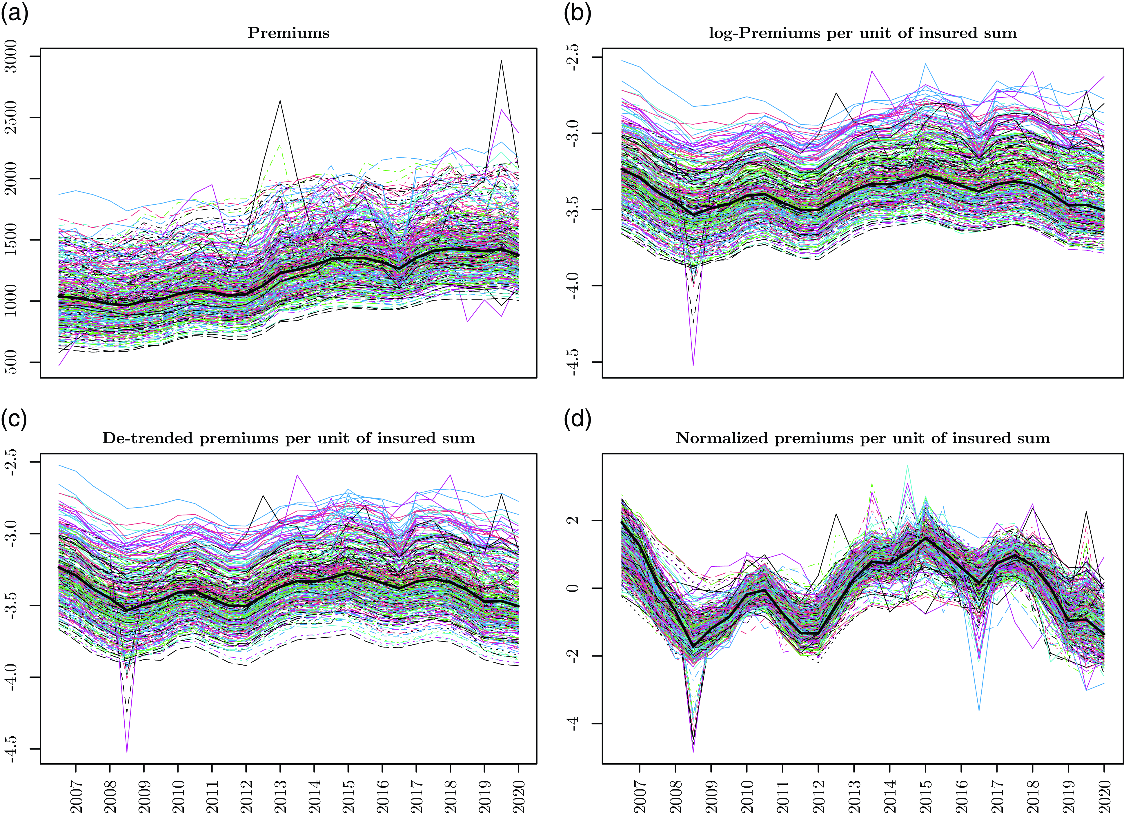
Fig. 1 displays (a) the original market average premiums, (b) the premiums divided by the insured sums (i.e. the price) on a logarithmic scale, (c) the price from (b) de-trended, and (d) the price from (c) normalized. All figures hint at the presence of cycles in the prices for the Brazilian motor insurance market. However, for some risk profiles, the data appears to be rather noisy. For instance, risk profiles from Rio Grande do Sul experienced a sharp drop in prices in the second semester of 2008, and males aged 18-25 from Rio de Janeiro and São Paulo experienced a milder drop in the second semester of 2016. Therefore, a systematic and automated method for cycle detection is required to ascertain the existence of cycles in insurance prices.
Premiums and prices per risk profile over time. Notes: (a) Top-left panel: original average premiums for 410 risk profiles from the AUTOSEG data set. (b) Top-right panel: corresponding premiums per unit of insured sums on a logarithmic scale. (c) Bottom-left panel: corresponding premiums per unit of insured sums (i.e. price) on a logarithmic scale, where prices for some risk profiles were de-trended, after which all time series passed the KPSS test of stationarity. (d) Bottom-right panel: corresponding prices after normalizing with the means and standard deviations.
3. Cycle detection methodologies
In this paper, a time series is considered cyclical if it is better modeled by an AR(2) process with complex roots or by a noisy sinusoid, rather than by an AR(0) or AR(1) process. This definition follows the standard approach in the underwriting cycle literature and is consistent with the methodologies evaluated in this study. Non-standard approaches such as AR processes with orders higher than 2, non-linear time series, or wavelet analysis, are not considered. Furthermore, heteroscedasticity is not accounted for, which is not a major omission for the paper’s application given that the results of the ARCH test do not provide strong support for the presence of heteroscedasticity in the time series.
This section outlines three methodologies used to detect cycles in times series. Subsection 3.1 describes the $g$
-test. Subsection 3.2 describes the methodology based on autoregressive models. Subsection 3.3 describes different NN models. The focus on the
$g$
-test. Subsection 3.2 describes the methodology based on autoregressive models. Subsection 3.3 describes different NN models. The focus on the $g$
-test and the AR models is motivated by the fact that they are the main approaches for cycle detection in the underwriting cycle literature, especially AR processes of orders up to 2.
$g$
-test and the AR models is motivated by the fact that they are the main approaches for cycle detection in the underwriting cycle literature, especially AR processes of orders up to 2.
3.1 Significance test for spectral peaks
One method to detect cyclicality in time series consists in visualizing their spectral densities; see Grace & Hotchkiss (Reference Grace and Hotchkiss1995) and Venezian & Leng (Reference Venezian and Leng2006) for applications in the context of the underwriting cycle. A spectral density function is a projection of the auto-correlation function from the time domain onto the frequency domain and is derived from a representation of time series using combinations of sinusoidal functions (Brockwell & Davis, Reference Brockwell and Davis2002). It is possible to detect cyclicality in time series if the spectral density has a peak at some given frequency.
When performing spectral analysis, a problem that may arise is that a spectral density function may have multiple peaks, and in such cases, it may be hard to draw sensible conclusions. Furthermore, carrying out a graphical analysis for each time series in the present analysis would be too cumbersome and not necessarily accurate. One way to automate the process, and to address the issue of spurious cycle detection, is to test the significance of spectral peaks (Lazar & Denuit, Reference Lazar and Denuit2012; Venezian, Reference Venezian2006). The $g$
-test proposed in Fisher (Reference Fisher1929) is one of the earliest methods applied for cycle detection, and it is still in use; see e.g. Lazar & Denuit (Reference Lazar and Denuit2012) for a review and application to the underwriting cycle.
$g$
-test proposed in Fisher (Reference Fisher1929) is one of the earliest methods applied for cycle detection, and it is still in use; see e.g. Lazar & Denuit (Reference Lazar and Denuit2012) for a review and application to the underwriting cycle.
The point estimate of the $g$
-test statistic is given by:
$g$
-test statistic is given by:
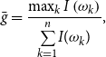 \begin{equation*}\bar {g}=\frac {\max _k I\left (\omega _k\right )}{\underset {k=1}{\overset {n}{\sum }}I(\omega _k)},\end{equation*}
with $n=\lfloor \frac {T-1}{2}\rfloor$
, and
$n=\lfloor \frac {T-1}{2}\rfloor$
, and $T$
is the number of observations, where
$T$
is the number of observations, where $I(\omega _k)$
is the periodogram at the discrete Fourier frequencies
$I(\omega _k)$
is the periodogram at the discrete Fourier frequencies $\omega _k=\frac {2\pi k}{T}$
, for
$\omega _k=\frac {2\pi k}{T}$
, for $k=0,1,\ldots, \lfloor \frac {T}{2}\rfloor$
, such that:
$k=0,1,\ldots, \lfloor \frac {T}{2}\rfloor$
, such that:
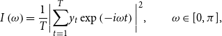 \begin{equation*}I\left (\omega \right ) = \frac {1}{T}\bigg |\underset {t=1}{\overset {T}{\sum }}y_t\exp \left (-i\omega t\right )\bigg |^2, \qquad \omega \in [0,\pi ],\end{equation*}
and $y_t$
is the time series under interest. Under the null hypothesis,
$y_t$
is the time series under interest. Under the null hypothesis, $y_t$
is a Gaussian white noise process. Large values of
$y_t$
is a Gaussian white noise process. Large values of $\bar {g}$
indicate that the highest peak of the spectral density, which is estimated by the periodogram, is significant, and hence lead to the rejection of the null hypothesis. Under the null hypothesis, the exact distribution of the
$\bar {g}$
indicate that the highest peak of the spectral density, which is estimated by the periodogram, is significant, and hence lead to the rejection of the null hypothesis. Under the null hypothesis, the exact distribution of the $g$
-test statistic is given by:
$g$
-test statistic is given by:
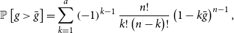 \begin{equation*}\mathbb{P}\left [g\gt \bar {g}\right ] = \underset {k=1}{\overset {a}{\sum }}\left (-1\right )^{k-1} \frac {n!}{k!\left (n-k\right )!}\left (1-k\bar {g}\right )^{n-1},\end{equation*}
where $a$
is the maximum integer less than
$a$
is the maximum integer less than $\frac {1}{\bar {g}}$
.
$\frac {1}{\bar {g}}$
.
3.2 Autoregressive models
Detecting cyclicality using second-order autoregressive processes, or AR(2), is the most common way in studies of the underwriting cycle (Cummins & Outreville, Reference Cummins and Outreville1987; Venezian, Reference Venezian1985). It is also the methodology criticized by Boyer et al. (Reference Boyer, Jacquier and Van Norden2012). In general, autoregressive processes exhibit cyclical behavior, provided the characteristic equation has complex roots. It follows that an autoregressive process of order 1 or less is not cyclical.
An AR(2) process has the following representation:
 \begin{equation} y_t = \phi _0 + \phi _1y_{t-1} + \phi _{2}y_{t-2} + \epsilon _{t}, \end{equation}
where $\epsilon _{t}$
is a white noise. The root of the characteristic equation is
$\epsilon _{t}$
is a white noise. The root of the characteristic equation is $\phi _1^2 + 4\phi _2$
, and hence, the process
$\phi _1^2 + 4\phi _2$
, and hence, the process $y_t$
is cyclical if
$y_t$
is cyclical if $\phi _1^2 + 4\phi _2\lt 0$
. In this case, the period of the cycle is
$\phi _1^2 + 4\phi _2\lt 0$
. In this case, the period of the cycle is $\frac {2\pi }{f}$
, where the expression of the frequency
$\frac {2\pi }{f}$
, where the expression of the frequency $f$
is
$f$
is $\arccos \left (\frac {0.5\phi _1}{\sqrt {-\phi _2}}\right )$
; see Cummins & Outreville (Reference Cummins and Outreville1987).
$\arccos \left (\frac {0.5\phi _1}{\sqrt {-\phi _2}}\right )$
; see Cummins & Outreville (Reference Cummins and Outreville1987).
Based on the properties of the process in (3.1), the classification of the time series into cyclical and non-cyclical premiums is achieved by fitting model (3.1) to the time series of interest, as well as the same model with $\phi _2=0$
or
$\phi _2=0$
or $\phi _2=\phi _1=0$
. The optimal model is chosen according to the value of the corrected Akaike Information Criteria (AICc):
$\phi _2=\phi _1=0$
. The optimal model is chosen according to the value of the corrected Akaike Information Criteria (AICc):
 \begin{equation*}\text{AICc}=T\log \left (\frac {1}{T}\sum \hat {\epsilon }_t^2\right ) + 2(k+1)+ \frac {2(k+1)(k+2)}{T-k-2},\end{equation*}
where $T$
is the number of observations, and
$T$
is the number of observations, and $k$
is the number of free parameters. For a given time series and for AR(p) with
$k$
is the number of free parameters. For a given time series and for AR(p) with $p\leq 2$
, if the model with the lowest AICc is not an AR(2) model, then the series is classified as non-cyclical. Otherwise, if the optimal model is an AR(2), the series is classified as cyclical if
$p\leq 2$
, if the model with the lowest AICc is not an AR(2) model, then the series is classified as non-cyclical. Otherwise, if the optimal model is an AR(2), the series is classified as cyclical if $\phi _1^2 + 4\phi _2\lt 0$
, and as non-cyclical otherwise.
$\phi _1^2 + 4\phi _2\lt 0$
, and as non-cyclical otherwise.
3.3 Neural networks
NNs are computational graphs that can extract mappings between inputs and targets. The extraction of mappings, or learning, occurs when the model is exposed to a sufficiently large amount of input-target pairs. NN models typically operate in layers, where each layer transforms the information distilled by the previous one. Each layer is parameterized by a set of weights, which are estimated during the learning phase. The estimation of the parameters is generally performed through a feedback mechanism, most commonly a gradient-based optimization with backpropagation, to determine the weights that minimize the error between the predictions and the actual targets (Aggrawal, Reference Aggrawal2018; Chollet & Allaire, Reference Chollet and Allaire2018; Rumelhart et al., Reference Rumelhart, Hinto and Williams1986). NNs have proven efficient in many actuarial applications, including forecasting mortality rates and modeling claims in non-life insurance for pricing and reserving (Gabrielli, Reference Gabrielli2020; Hainaut, Reference Hainaut2018; Li, Reference Li2022; Lindholm et al., Reference Lindholm, Richman, Tsanakas and Wüthrich2022; Shi and Shi, Reference Shi and Shi2022). In the present context, the goal is to classify the series as either cyclical or non-cyclical.
NN models need to be trained using data for which both input and output are known before they are applied for predictions, i.e. in situations where the output is unknown. The data for which both input and output are known are used to update the parameters of the model and to tune its hyperparameters (i.e. the set of defining features of the network, including its structure and the way it learns). The next section describes how several data sets are simulated. The simulated data are used to train the NN models, as well as to compare the performance of the three cycle detection methodologies (the $g$
-test, autoregressive processes, and NN models).
$g$
-test, autoregressive processes, and NN models).
Four NN architectures are considered in this study. The architectures are determined using the simulated data described in the next subsection. Hyperparameter tuning is based on standard best-practice methods by monitoring the accuracy of the validation sets. The first model is a fully connected NN (FNN) and consists of fully connected layers only. It has four hidden layers, with number of nodes 512, 512, 64, and 8, and dropout rates of 0.4 at each layer. The second model is a recurrent NN (RNN). It has two identical bidirectional Gated Recurrent Unit (GRU) layers with 256 units each, a dropout rate of 0.1, and a recurrent dropout rate of 0.5. The output of the recurrent base of the network is flattened and then processed through a fully connected layer with 256 units, and a dropout rate of 0.1. The third model is a one-dimensional convolutional NN (CNN). It has two convolution layers with 512 and 256 filters of size 25, respectively. A stride of 2 is used with zero padding. The output of the convolution base is flattened into a first fully connected layer with 128 units and a dropout rate of 0.1, and then a second fully connected layer with 64 units and a dropout rate of 0.2. The fourth model is a hybrid convolutional-recurrent architecture. It starts with a one-dimensional convolution layer with 512 filers with size 20, and a stride of 2 with zero-padding. The convolution layer is followed by a bidirectional GRU layer with 128 units, a dropout rate of 0.1, and a recurrent dropout rate of 0.5. The recurrent layer of the hybrid NN is connected to the final single-node output layer through a fully connected layer with 32 units and a dropout rate of 0.1.
For all architectures, the target function for calibration is binary cross-entropy, which is standard for classification tasks. The output layer consists of a single neuron with a sigmoid activation function, producing a probability score for each series. A threshold of 0.5 is used to classify a series as cyclical or non-cyclical. The input to the NN consists of the full-time series, represented as a vector of 28 observations corresponding to the length of each sample in the data set. Models are trained using the Adam optimizer with early stopping to prevent overfitting, and the number of epochs is set to 30 based on validation performance.
It is worth noting that given the number of parameters in NN models, overfitting is a potential concern. However, several measures are implemented to mitigate this risk. First, dropout regularization, as described above, prevents the networks from relying too heavily on specific neurons. Second, the size of the training set is sufficiently large relative to the number of parameters, with thousands of time series providing diverse patterns for robust learning. Last, the performance of the models is evaluated on completely unseen test data, confirming that improvements in cycle detection are not artifacts of overfitting but rather genuine enhancements in identifying cyclical patterns.
4. Simulation study
The goal of this subsection is to compare the performance of the different methodologies on simulated data. It is structured in three parts. Subsection 4.1 describes the design of the simulation study. Subsection 4.2 provides details on the procedure for simulating different data sets. Subsection 4.3 reports the results of the simulation study. Recall that the simulated data sets serve two purposes. The first purpose of the simulated data sets is to compare the efficacy of all methodologies ( $g$
-test, AR processes, and the four NN models) in cycle detection. The results of this analysis are reported in Subsection 4.3. The second purpose of the simulated data sets is to train the NN models for the empirical application of the paper. Specifically, the NN’s models learn to detect cyclicality in the simulated data before they are applied to the Brazilian data. These latter results are reported in Section 5.
$g$
-test, AR processes, and the four NN models) in cycle detection. The results of this analysis are reported in Subsection 4.3. The second purpose of the simulated data sets is to train the NN models for the empirical application of the paper. Specifically, the NN’s models learn to detect cyclicality in the simulated data before they are applied to the Brazilian data. These latter results are reported in Section 5.
4.1 Design of the simulation
Standard best-practice methods to evaluate the efficacy of NN models prescribe using three different data sets. The training and validation sets, which are used to train and fine-tune the architectures, and the test data set, which is used to compare the performance of the models. In order to ensure that the performance of the NNs on the test data is not due to over-fitting or to the similarity of that data set with the training data, the three data sets should be disjoint.
The simulation study in this paper uses five sets of data generating processes $\mathcal{G}_i$
,
$\mathcal{G}_i$
, $i=1,\ldots, 5$
, to generate five data sets
$i=1,\ldots, 5$
, to generate five data sets $\mathcal{S}_i$
. Each data set
$\mathcal{S}_i$
. Each data set $\mathcal{S}_i$
contains a mix of cyclical AR(2) and non-cyclical AR(1) and AR(0). The series across the different sets
$\mathcal{S}_i$
contains a mix of cyclical AR(2) and non-cyclical AR(1) and AR(0). The series across the different sets $\mathcal{S}_i$
are grouped by the parameters of the AR(p) processes. Namely, each set contains cyclical time series with specific range of values of cycle periods, AR(1) time series with specific range of values of the parameter
$\mathcal{S}_i$
are grouped by the parameters of the AR(p) processes. Namely, each set contains cyclical time series with specific range of values of cycle periods, AR(1) time series with specific range of values of the parameter $\phi _1$
, and AR(0) time-series with specific range of values of standard deviations. In particular,
$\phi _1$
, and AR(0) time-series with specific range of values of standard deviations. In particular, $\mathcal{S}_1$
is associated with “low” values,
$\mathcal{S}_1$
is associated with “low” values, $\mathcal{S}_2$
is associated with “medium-low” values,
$\mathcal{S}_2$
is associated with “medium-low” values, $\mathcal{S}_3$
is associated with “medium-high” values and
$\mathcal{S}_3$
is associated with “medium-high” values and $\mathcal{S}_4$
is associated with “high” values. All intermediary values, as well as “very low” and “very high” values are included in
$\mathcal{S}_4$
is associated with “high” values. All intermediary values, as well as “very low” and “very high” values are included in $\mathcal{S}_5$
. This procedure ensures that the overlap between the sets
$\mathcal{S}_5$
. This procedure ensures that the overlap between the sets $\mathcal{S}_1$
,
$\mathcal{S}_1$
, $\mathcal{S}_2$
,
$\mathcal{S}_2$
, $\mathcal{S}_3$
and
$\mathcal{S}_3$
and $\mathcal{S}_4$
is significantly reduced.
$\mathcal{S}_4$
is significantly reduced.
The first step is to determine the hyperparameters of the NN models (e.g. the number and size of layers). Note that fixing the hyperparameters and estimating the weights of the NN models are two different tasks, and the latter task is referred to here as “training.” In this first step, where the hyperparameters are determined, $\mathcal{S}_1$
and
$\mathcal{S}_1$
and $\mathcal{S}_4$
are used as training data, and
$\mathcal{S}_4$
are used as training data, and $\mathcal{S}_3$
is used as validation data to tune the hyperparameters of the NNs. The second step is to study the performance of all methodologies (
$\mathcal{S}_3$
is used as validation data to tune the hyperparameters of the NNs. The second step is to study the performance of all methodologies ( $g$
-test, autoregressive models, and NNs) in detecting different types of cyclicality. In particular, using the NN architectures obtained from Step 1, the simulation study is structured as follows:
$g$
-test, autoregressive models, and NNs) in detecting different types of cyclicality. In particular, using the NN architectures obtained from Step 1, the simulation study is structured as follows:
-
(a) train the NN models on $\mathcal{S}_2$
,
$\mathcal{S}_3$
and
$\mathcal{S}_4$
, and test all methods on
$\mathcal{S}_1$
(low).
$\mathcal{S}_2$
,
$\mathcal{S}_3$
and
$\mathcal{S}_4$
, and test all methods on
$\mathcal{S}_1$
(low). -
(b) train the NN models on
$\mathcal{S}_1$
,
$\mathcal{S}_3$
and
$\mathcal{S}_4$
and test all methods on
$\mathcal{S}_2$
(medium-low). -
(c) train the NN models on
$\mathcal{S}_1$
,
$\mathcal{S}_2$
and
$\mathcal{S}_4$
and test all methods on
$\mathcal{S}_3$
(medium-high). -
(d) train the NN models on
$\mathcal{S}_1$
,
$\mathcal{S}_2$
and
$\mathcal{S}_3$
and test all methods on
$\mathcal{S}_4$
(high). -
(e) train the NN models on
$\mathcal{S}_1$
,
$\mathcal{S}_2$
,
$\mathcal{S}_3$
and
$\mathcal{S}_4$
and test all methods on
$\mathcal{S}_5$
(intermediary and extreme).


Note again that the architectures of the NN models are determined using $\mathcal{S}_1$
,
$\mathcal{S}_1$
, $\mathcal{S}_3$
and
$\mathcal{S}_3$
and $\mathcal{S}_4$
, but the parameters of each architecture are different for each test and depend on the training data used. Note also that in each test, the data used in the comparison of the methodologies are different from those on which the NN models are trained.
$\mathcal{S}_4$
, but the parameters of each architecture are different for each test and depend on the training data used. Note also that in each test, the data used in the comparison of the methodologies are different from those on which the NN models are trained.
4.2 Simulated data
This subsection explains how the simulated data are obtained. First, a decomposition procedure is applied to the AUTOSEG data to obtain a larger sample of parameters of both cyclical and non-cyclical AR(p) models. This is because the NN models will be applied to detect cyclicality in the Brazilian insurance industry, and a resemblance between the simulated and the available data will increase the reliability of the NNs. Second, the sets of estimated parameters are augmented by fitting a multivariate model to the estimated ones and simulating a large number of new parameters from that multivariate distribution. Third, the data-generating processes are assigned to the sets $\mathcal{G}_i$
using a splitting approach that attempts to avoid overlap between the sets. Fourth, within each of these five sets, the cyclical data-generating processes based on AR(2) models are supplemented with cosine-based models. Fifth, the data are simulated and normalized using the means and standard deviations. The remainder of this subsection provides details on each of these five steps.
$\mathcal{G}_i$
using a splitting approach that attempts to avoid overlap between the sets. Fourth, within each of these five sets, the cyclical data-generating processes based on AR(2) models are supplemented with cosine-based models. Fifth, the data are simulated and normalized using the means and standard deviations. The remainder of this subsection provides details on each of these five steps.
4.2.1 Step 1 – STL decomposition
In order to increase the available data, each of the AUTOSEG time series of prices is filtered using Cleveland et al. (Reference Cleveland, Cleveland, McRae and Terpenning1990) seasonal-trend (STL) procedure to separate the trend and the remainder components. Note that since the data is bi-annual, the seasonal component is insignificant, and hence, the outcome of the STL decomposition for each series of the AUTOSEG is one cyclical series and a remainder non-cyclical series. The autoregressive process in (3.1), as well as the nested models with $\phi _2=0$
or
$\phi _2=0$
or $\phi _2=\phi _1=0$
, are estimated for each series, and the optimal model is selected based on the AICc. All of the 410 trend components series except two are better modeled with AR(2) cyclical processes, whereas all of the 410 remainder components series are better modeled with either AR(1) or AR(0) processes. This results in 818 sets of parameters
$\phi _2=\phi _1=0$
, are estimated for each series, and the optimal model is selected based on the AICc. All of the 410 trend components series except two are better modeled with AR(2) cyclical processes, whereas all of the 410 remainder components series are better modeled with either AR(1) or AR(0) processes. This results in 818 sets of parameters $\left (\hat {\phi }_0,\hat {\phi }_1,\hat {\phi }_2,\hat {\sigma }\right )$
with no duplicates, where
$\left (\hat {\phi }_0,\hat {\phi }_1,\hat {\phi }_2,\hat {\sigma }\right )$
with no duplicates, where $\hat {\sigma }$
is the standard deviation of the residuals, and
$\hat {\sigma }$
is the standard deviation of the residuals, and $\hat {\phi }_2\lt 0$
and
$\hat {\phi }_2\lt 0$
and $\hat {\phi }_1+4\hat {\phi }_2\lt 0$
for all AR(2) processes. Since all series are normalized,
$\hat {\phi }_1+4\hat {\phi }_2\lt 0$
for all AR(2) processes. Since all series are normalized, $\phi _0$
is set to
$\phi _0$
is set to $0$
.
$0$
.
4.2.2 Step 2 – Multivariate distribution for simulating new parameters
The vector $\left (\log \left (\hat {\phi }_1\right ),\log \left (-\hat {\phi }_2\right ),\sqrt {\hat {\sigma }}\right )$
of estimated parameters from the AR(2) processes and its counterpart
$\left (\log \left (\hat {\phi }_1\right ),\log \left (-\hat {\phi }_2\right ),\sqrt {\hat {\sigma }}\right )$
of estimated parameters from the AR(2) processes and its counterpart $\left (\log \left (\hat {\phi }_1\right ),\sqrt {\hat {\sigma }}\right )$
from the AR(1) processes are modeled using a variance gamma for the marginal distributions and a vine copula for the dependence structure. These models are used to generate 10,000 new sets of AR(2) parameters
$\left (\log \left (\hat {\phi }_1\right ),\sqrt {\hat {\sigma }}\right )$
from the AR(1) processes are modeled using a variance gamma for the marginal distributions and a vine copula for the dependence structure. These models are used to generate 10,000 new sets of AR(2) parameters $\left (\tilde {\phi }_1,\tilde {\phi }_2,\tilde {\sigma }\right )$
satisfying the condition of cyclicality, and another 10,000 of AR(1) parameters. For the AR(0) processes, 10,000 parameters
$\left (\tilde {\phi }_1,\tilde {\phi }_2,\tilde {\sigma }\right )$
satisfying the condition of cyclicality, and another 10,000 of AR(1) parameters. For the AR(0) processes, 10,000 parameters $\tilde {\sigma }$
are simulated assuming that the estimated
$\tilde {\sigma }$
are simulated assuming that the estimated $\sqrt {\hat {\sigma }}$
follow a variance gamma distribution. The choice of the marginal distributions and log transformations was based on a visual inspection of the Q-Q plots, and the selection of the copulas is based on a comparison of the AIC.
$\sqrt {\hat {\sigma }}$
follow a variance gamma distribution. The choice of the marginal distributions and log transformations was based on a visual inspection of the Q-Q plots, and the selection of the copulas is based on a comparison of the AIC.
4.2.3 Step 3 – Assignment of the parameters
In order to ensure that the training, validation, and test data are disjoint, the parameters $\left (\tilde {\phi }_1,\tilde {\phi }_2,\tilde {\sigma }\right )$
must be split before the simulations. The typical approach for splitting the data is to randomly assign proportions for each set. In the present context, this approach could assign similar parameters across the three data sets, which would violate the requirement of disjoint sets.
$\left (\tilde {\phi }_1,\tilde {\phi }_2,\tilde {\sigma }\right )$
must be split before the simulations. The typical approach for splitting the data is to randomly assign proportions for each set. In the present context, this approach could assign similar parameters across the three data sets, which would violate the requirement of disjoint sets.
The approach followed here for splitting the data-generating processes attempts to ensure that the sets are disjoint and allows to evaluate the performance of the models in detecting different types of cyclicality (e.g. cycles with low or high periods). For the AR(2) processes, this is achieved by assigning the parameters based on the value of their associated cycle period. Those values are first split into several bins based on their quantile values. The bins are then allocated to the sets $\mathcal{G}_i$
for
$\mathcal{G}_i$
for $i=1,\ldots, 5$
. A similar procedure is performed for the sets of parameters of the non-cyclical processes, where the reference quantities used for the partitioning are the values of
$i=1,\ldots, 5$
. A similar procedure is performed for the sets of parameters of the non-cyclical processes, where the reference quantities used for the partitioning are the values of $\tilde {\phi }_1$
for the AR(1), and
$\tilde {\phi }_1$
for the AR(1), and $\tilde {\sigma }$
for the AR(0).
$\tilde {\sigma }$
for the AR(0).
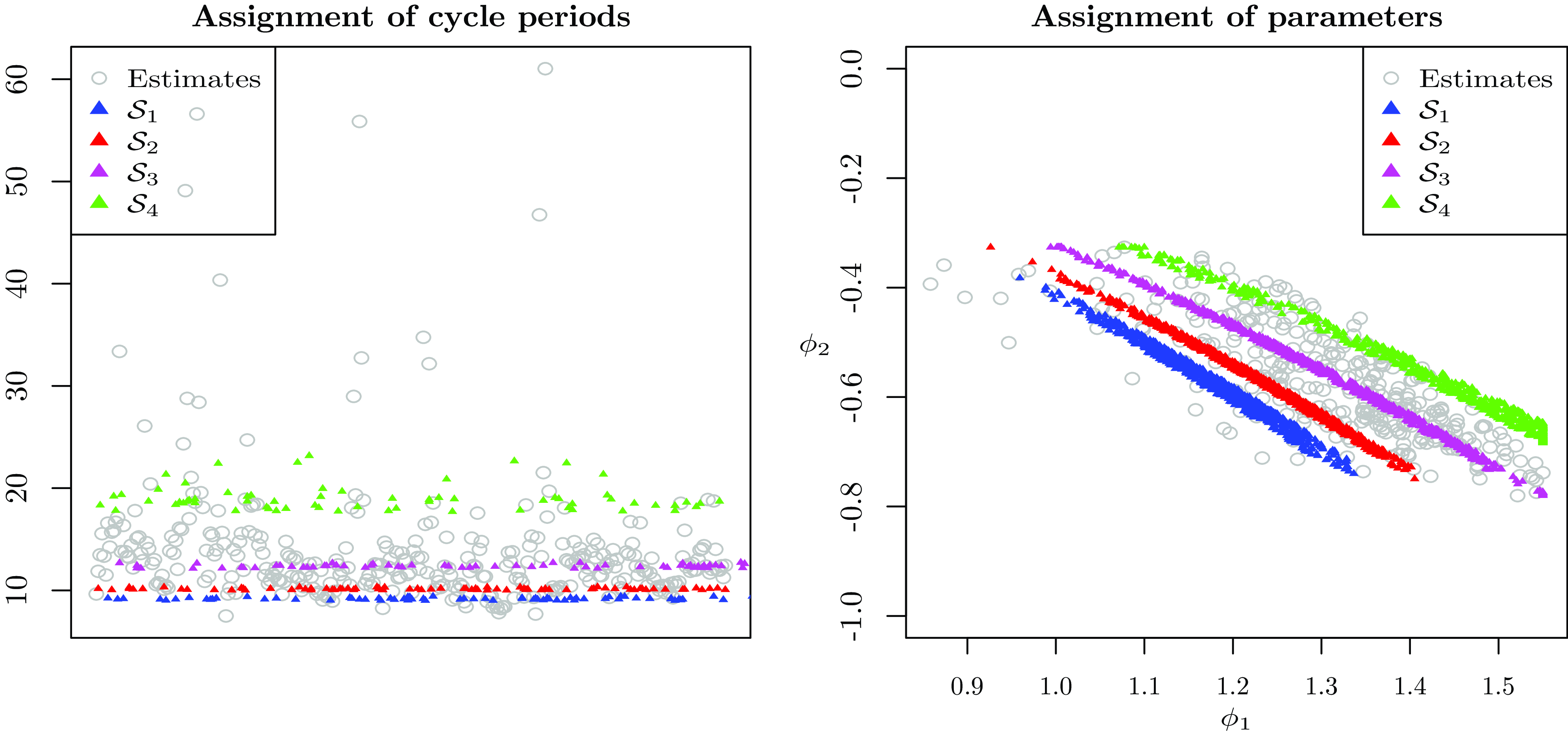
Fig. 2 shows how the partitioning is performed for the AR(2) processes. On the left panel, the figure displays the estimated cycle periods $\frac {2\pi }{\hat {f}}$
(gray circles) and the assignment of the simulated cycle periods
$\frac {2\pi }{\hat {f}}$
(gray circles) and the assignment of the simulated cycle periods $\frac {2\pi }{\tilde {f}}$
into
$\frac {2\pi }{\tilde {f}}$
into $\mathcal{G}_1$
(blue triangles),
$\mathcal{G}_1$
(blue triangles), $\mathcal{G}_2$
(red triangles),
$\mathcal{G}_2$
(red triangles), $\mathcal{G}_3$
(magenta triangles) and
$\mathcal{G}_3$
(magenta triangles) and $\mathcal{G}_4$
(green triangles). On the right panel, the figure displays the corresponding estimated parameters
$\mathcal{G}_4$
(green triangles). On the right panel, the figure displays the corresponding estimated parameters $\left (\hat {\phi }_1,\hat {\phi }_2\right )$
(gray circles) and the assignment of the simulated parameters
$\left (\hat {\phi }_1,\hat {\phi }_2\right )$
(gray circles) and the assignment of the simulated parameters $\mathcal{G}_1$
(blue triangles),
$\mathcal{G}_1$
(blue triangles), $\mathcal{G}_2$
(red triangles),
$\mathcal{G}_2$
(red triangles), $\mathcal{G}_3$
(magenta triangles) and
$\mathcal{G}_3$
(magenta triangles) and $\mathcal{G}_4$
(green triangles). The figure shows that there is no overlap between the sets in terms of cycle periods. The figure also shows that the simulated parameters are consistent with those estimated from the Brazilian data sets.
$\mathcal{G}_4$
(green triangles). The figure shows that there is no overlap between the sets in terms of cycle periods. The figure also shows that the simulated parameters are consistent with those estimated from the Brazilian data sets.
Assignment of parameters for the simulated data. Notes: This figure displays the split of the parameters into $\mathcal{G}_i$
for
$\mathcal{G}_i$
for $i=1,\ldots 4$
. On the left panel, the figure displays the estimated cycle periods
$i=1,\ldots 4$
. On the left panel, the figure displays the estimated cycle periods $\frac {2\pi }{\hat {f}}$
(gray circles) of the cyclical trend components, and the assignment of the simulated cycle periods
$\frac {2\pi }{\hat {f}}$
(gray circles) of the cyclical trend components, and the assignment of the simulated cycle periods $\frac {2\pi }{\tilde {f}}$
into
$\frac {2\pi }{\tilde {f}}$
into $\mathcal{G}_1$
(blue triangles),
$\mathcal{G}_1$
(blue triangles), $\mathcal{G}_2$
(red triangles),
$\mathcal{G}_2$
(red triangles), $\mathcal{G}_3$
(magenta triangles) and
$\mathcal{G}_3$
(magenta triangles) and $\mathcal{G}_4$
(green triangles). On the right panel, the figure displays the corresponding estimated parameters
$\mathcal{G}_4$
(green triangles). On the right panel, the figure displays the corresponding estimated parameters $(\hat {\phi }_1,\hat {\phi }_2)$
(gray circles) and the assignment of the simulated parameters
$(\hat {\phi }_1,\hat {\phi }_2)$
(gray circles) and the assignment of the simulated parameters $(\tilde {\phi }_1,\tilde {\phi }_2)$
into
$(\tilde {\phi }_1,\tilde {\phi }_2)$
into $\mathcal{G}_1$
(blue triangles),
$\mathcal{G}_1$
(blue triangles), $\mathcal{G}_2$
(red triangles),
$\mathcal{G}_2$
(red triangles), $\mathcal{G}_3$
(magenta triangles) and
$\mathcal{G}_3$
(magenta triangles) and $\mathcal{G}_4$
(green triangles).
$\mathcal{G}_4$
(green triangles).
4.2.4 Step 4 – Cyclical data generating processes using cosines
A cyclical data generating process given by $\beta \cos \left (\omega t \right ) + \epsilon _t$
is added, where
$\beta \cos \left (\omega t \right ) + \epsilon _t$
is added, where $\epsilon _t$
has a standard deviation
$\epsilon _t$
has a standard deviation $\tilde {\sigma }$
. The standard deviation
$\tilde {\sigma }$
. The standard deviation $\tilde {\sigma }$
is sampled from those of the AR(2), and
$\tilde {\sigma }$
is sampled from those of the AR(2), and $\beta$
is uniformly drawn from
$\beta$
is uniformly drawn from $[0.5,5.5]$
. The parameter
$[0.5,5.5]$
. The parameter $\omega$
is such that the period
$\omega$
is such that the period $\frac {2\pi }{\omega }$
is consistent with
$\frac {2\pi }{\omega }$
is consistent with $\frac {2\pi }{\tilde {f}}$
from the relevant set
$\frac {2\pi }{\tilde {f}}$
from the relevant set $\mathcal{G}_i$
.
$\mathcal{G}_i$
.
4.2.5 Step 5 – Data simulation
For each set of parameters, several paths are simulated, assuming that $\epsilon _t$
has either a normal distribution with standard deviation
$\epsilon _t$
has either a normal distribution with standard deviation $\tilde {\sigma }$
, or a
$\tilde {\sigma }$
, or a $t$
distribution with degree of freedom
$t$
distribution with degree of freedom $\nu =2.5$
and scaled by
$\nu =2.5$
and scaled by $\frac {\tilde {\sigma }}{\sqrt {5}}$
. Scaling by
$\frac {\tilde {\sigma }}{\sqrt {5}}$
. Scaling by $\frac {\tilde {\sigma }}{\sqrt {5}}$
in case of
$\frac {\tilde {\sigma }}{\sqrt {5}}$
in case of $t$
distributed errors ensures the standard deviation of the process is equal to
$t$
distributed errors ensures the standard deviation of the process is equal to $\tilde {\sigma }$
. For each path, the number of observations is randomly chosen between
$\tilde {\sigma }$
. For each path, the number of observations is randomly chosen between $50$
and
$50$
and $150$
, but only the last 28 observations are selected. This allows us to obtain asynchronous paths. Each data set
$150$
, but only the last 28 observations are selected. This allows us to obtain asynchronous paths. Each data set $\mathcal{S}_i$
for
$\mathcal{S}_i$
for $i=1,\ldots, 5$
contains 2,000 paths from the cyclical AR processes with normally distributed errors, 2,000 paths from the cyclical AR processes with
$i=1,\ldots, 5$
contains 2,000 paths from the cyclical AR processes with normally distributed errors, 2,000 paths from the cyclical AR processes with $t$
distributed errors, 2,000 paths from the cosine process, 3,000 paths from the non-cyclical AR processes (either AR(0) or AR(1)) with normally distributed errors, and 3,000 paths from the non-cyclical AR processes (either AR(0) or AR(1)) with
$t$
distributed errors, 2,000 paths from the cosine process, 3,000 paths from the non-cyclical AR processes (either AR(0) or AR(1)) with normally distributed errors, and 3,000 paths from the non-cyclical AR processes (either AR(0) or AR(1)) with $t$
distributed errors. In particular, each data set contains the same number of time series from each class, namely 6,000 cyclical time series and 6,000 non-cyclical ones. This means that the binary classification problem is balanced (i.e. 50% of series in each class), and hence, that the classification accuracy is an appropriate measure to evaluate the performance of the models. Each simulated path is normalized individually by subtracting its mean and dividing by its standard deviation.
$t$
distributed errors. In particular, each data set contains the same number of time series from each class, namely 6,000 cyclical time series and 6,000 non-cyclical ones. This means that the binary classification problem is balanced (i.e. 50% of series in each class), and hence, that the classification accuracy is an appropriate measure to evaluate the performance of the models. Each simulated path is normalized individually by subtracting its mean and dividing by its standard deviation.
4.2.6 Software use
The analysis is conducted on R using the packages tseries and seasonal for time series analyses, the packages VarianceGamma and rvinecopulib for the multivariate modeling of the parameters, and the packages keras, kerasR and tensorflow for fitting the NNs. The code that supports the findings of this study is available on request from the author.
4.3 Results of the simulation study
4.3.1 Results on the test data sets
Table 1 reports the accuracy rate, the true positive rate (sensitivity), and the true negative rate (specificity) of all methodologies for different levels of cyclicality. Note that when the test data set $\mathcal{S}_j$
for
$\mathcal{S}_j$
for $j=1,\ldots 4$
is evaluated, the training data set for the NN models is
$j=1,\ldots 4$
is evaluated, the training data set for the NN models is $\underset {1\leq i \leq 4}{\cup }\mathcal{S}_i \setminus \mathcal{S}_j$
, whereas when the test data set
$\underset {1\leq i \leq 4}{\cup }\mathcal{S}_i \setminus \mathcal{S}_j$
, whereas when the test data set $\mathcal{S}_5$
is evaluated, the training data set is
$\mathcal{S}_5$
is evaluated, the training data set is $\underset {1\leq i \leq 4}{\cup }\mathcal{S}_i$
. The results for the
$\underset {1\leq i \leq 4}{\cup }\mathcal{S}_i$
. The results for the $g$
-test are reported with and without Bonferroni correction for multiple-comparison, where the threshold for the
$g$
-test are reported with and without Bonferroni correction for multiple-comparison, where the threshold for the $p$
-value is set to the conventional significance level of
$p$
-value is set to the conventional significance level of $0.05$
.
$0.05$
.
Accuracy, sensitivity, and specificity of all methodologies on different simulated test data
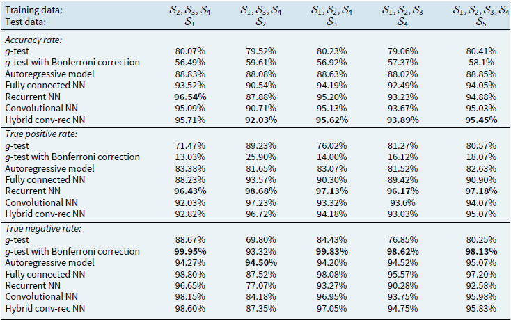
Notes: This table reports the accuracy rate, the true positive rate (sensitivity) and the true negative rate (specificity) of all methodologies on the test data $\mathcal{S}_j$
when the training data set is
$\mathcal{S}_j$
when the training data set is $\cup _{1\leq i \leq 4}\mathcal{S}_i \setminus \mathcal{S}_j$
, for
$\cup _{1\leq i \leq 4}\mathcal{S}_i \setminus \mathcal{S}_j$
, for $j=1,2,3,4$
, as well as the performance on the test data
$j=1,2,3,4$
, as well as the performance on the test data $\mathcal{S}_5$
when the training data set is
$\mathcal{S}_5$
when the training data set is $\cup _{1\leq i \leq 4}\mathcal{S}_i$
. The highest value of each measure and data set across all models is highlighted in bold.
$\cup _{1\leq i \leq 4}\mathcal{S}_i$
. The highest value of each measure and data set across all models is highlighted in bold.
Looking first at the accuracy rate, overall, the four NN models outperform both the $g$
-test and autoregressive processes in terms of cycle detection on all data sets. Furthermore, the hybrid convolutional-recurrent model outperforms the other NN models with higher accuracy on all data sets except for
$g$
-test and autoregressive processes in terms of cycle detection on all data sets. Furthermore, the hybrid convolutional-recurrent model outperforms the other NN models with higher accuracy on all data sets except for $\mathcal{S}_1$
(i.e. low cycle period). The accuracy rates of the top-performing model vary across the data sets, where the lowest value is
$\mathcal{S}_1$
(i.e. low cycle period). The accuracy rates of the top-performing model vary across the data sets, where the lowest value is $92.03\%$
on
$92.03\%$
on $\mathcal{S}_2$
(i.e. medium-low cycle period), and the highest value is
$\mathcal{S}_2$
(i.e. medium-low cycle period), and the highest value is $96.54\%$
on
$96.54\%$
on $\mathcal{S}_1$
(i.e. low cycle period).
$\mathcal{S}_1$
(i.e. low cycle period).
Regarding the $g$
-test and autoregressive processes, two observations are noteworthy. The first observation is that, whereas the
$g$
-test and autoregressive processes, two observations are noteworthy. The first observation is that, whereas the $g$
-test has the lowest accuracy rates, those values tend to decrease significantly when the Bonferroni correction is applied. This result suggests that Bonferroni correction is not necessarily useful in the present context. The second observation is that despite the criticism expressed by Boyer et al. (Reference Boyer, Jacquier and Van Norden2012), the methodology based on AR processes performs satisfactorily with an average accuracy of about
$g$
-test has the lowest accuracy rates, those values tend to decrease significantly when the Bonferroni correction is applied. This result suggests that Bonferroni correction is not necessarily useful in the present context. The second observation is that despite the criticism expressed by Boyer et al. (Reference Boyer, Jacquier and Van Norden2012), the methodology based on AR processes performs satisfactorily with an average accuracy of about $88.5\%$
across the five data sets. Nevertheless, as it is shown later in this section, the performance of the AR(p) model deteriorates significantly when outliers and structural breaks are present in the data.
$88.5\%$
across the five data sets. Nevertheless, as it is shown later in this section, the performance of the AR(p) model deteriorates significantly when outliers and structural breaks are present in the data.
The true positive rate is highest for recurrent NN model, where its performance is closely matched by the convolutional and hybrid networks. That performance is also associated with the lowest true negative rate among the NN models. On the other hand, the true negative rate is highest for the $g$
-test with Bonferroni correction, which is close to 100%, but it comes at the cost of too low true positive rates. This is because the
$g$
-test with Bonferroni correction, which is close to 100%, but it comes at the cost of too low true positive rates. This is because the $g$
-test with Bonferroni correction classifies most series as non-cyclical, which leads to a high specificity but a low sensitivity.
$g$
-test with Bonferroni correction classifies most series as non-cyclical, which leads to a high specificity but a low sensitivity.
The results from Table 1 based on simulated data highlight the high performance of NNs in distinguishing between cosines with noise or AR(2) from AR(1)/AR(0) process, which substantially exceeds that of the $g$
-test and autoregressive models. Furthermore, among the four NN models, the hybrid convolutional-recurrent architecture has a higher efficacy in cycle detection, even though the performance measures of all four architectures are close. Interestingly, the NN models perform better than AR(p) models despite the data being generated from AR(p) and cosine-based models.
$g$
-test and autoregressive models. Furthermore, among the four NN models, the hybrid convolutional-recurrent architecture has a higher efficacy in cycle detection, even though the performance measures of all four architectures are close. Interestingly, the NN models perform better than AR(p) models despite the data being generated from AR(p) and cosine-based models.
4.3.2 Ensembling
An additional test is performed, consisting of fitting a weighted average of the predictions from the $g$
-test, autoregressive processes, and the four NN models. This ensembling is performed for each of the five data sets
$g$
-test, autoregressive processes, and the four NN models. This ensembling is performed for each of the five data sets $\underset {1\leq i \leq 4}{\cup }\mathcal{S}_i \setminus \mathcal{S}_j$
, for
$\underset {1\leq i \leq 4}{\cup }\mathcal{S}_i \setminus \mathcal{S}_j$
, for $j=1,2,3,4$
and
$j=1,2,3,4$
and $\underset {1\leq i \leq 4}{\cup }\mathcal{S}_i$
. The goal is to verify whether combining the different methodologies could help to further improve the detection of cycles. The estimated weights are reported in Table 2, where the values are estimated by minimizing the sum of squared differences between the predictions from the ensemble and the targets from the relevant training set. Note that the ensembling performed using the binary cross-entropy leads to similar conclusions.
$\underset {1\leq i \leq 4}{\cup }\mathcal{S}_i$
. The goal is to verify whether combining the different methodologies could help to further improve the detection of cycles. The estimated weights are reported in Table 2, where the values are estimated by minimizing the sum of squared differences between the predictions from the ensemble and the targets from the relevant training set. Note that the ensembling performed using the binary cross-entropy leads to similar conclusions.
Estimated weights from ensembling all models
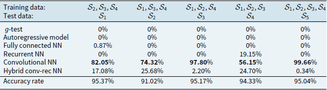
Notes: This table reports the estimated weights on each method ( $g$
-test, autoregressive model, and NN’s) obtained by minimizing the sum of squared differences between the predictions from the ensemble and the targets from the relevant training set
$g$
-test, autoregressive model, and NN’s) obtained by minimizing the sum of squared differences between the predictions from the ensemble and the targets from the relevant training set $\cup _{1\leq i \leq 4}\mathcal{S}_i \setminus \mathcal{S}_j$
, for
$\cup _{1\leq i \leq 4}\mathcal{S}_i \setminus \mathcal{S}_j$
, for $j=1,2,3,4$
, and
$j=1,2,3,4$
, and $\cup _{1\leq i \leq 4}\mathcal{S}_i$
.
$\cup _{1\leq i \leq 4}\mathcal{S}_i$
.
The first observation from Table 2 is that for all data sets, the $g$
-test and the autoregressive model are assigned weights of
$g$
-test and the autoregressive model are assigned weights of $0\%$
. This suggests that not only are the NN models able to detect cyclicality with high accuracy, but that additional input from the
$0\%$
. This suggests that not only are the NN models able to detect cyclicality with high accuracy, but that additional input from the $g$
-test and autoregressive processes is not necessary on the training data. The second observation is that, among the NN models, the convolutional NN is assigned the highest weight on all training data sets. The hybrid model comes second, and the recurrent NN comes third, where it is assigned a positive weight for one data set only. The FNN is not used at all.
$g$
-test and autoregressive processes is not necessary on the training data. The second observation is that, among the NN models, the convolutional NN is assigned the highest weight on all training data sets. The hybrid model comes second, and the recurrent NN comes third, where it is assigned a positive weight for one data set only. The FNN is not used at all.
It is worth mentioning that these weights are determined using the training data, and hence, this result does not necessarily mean that the convolutional NN is the best model on the unseen test data. Indeed, as discussed in the previous subsection, Table 1 shows that the hybrid convolutional-recurrent NN outperforms the other models on 4 out of the 5 test data sets, whereas the recurrent NN outperforms the other models on the remaining data set. In Table 2, the accuracy rates on the test data show that the ensembles outperform the convolutional NN, but the accuracy rates are still lower compared to those of the hybrid convolutional-recurrent NN.
4.3.3 Performance in the presence of outliers and structural breaks
In order to provide deeper understanding of the differences between the methodologies in terms of cycle detection, this subsection investigates the cycle detection power of all methodologies when the time series contain either outliers or structural breaks in the mean. Understanding the cycle detection ability of all models in such cases is important, as Fig. 1 suggests that some time series exhibit those features.
Let $y_t$
be a simulated time series from any of the data sets
$y_t$
be a simulated time series from any of the data sets $\mathcal{S}_i$
. Recall that the series were standardized, such that their mean is 0 and their standard deviation is 1. The corresponding time series
$\mathcal{S}_i$
. Recall that the series were standardized, such that their mean is 0 and their standard deviation is 1. The corresponding time series $y_t^{outlier}(s,\delta )$
is the transformation of
$y_t^{outlier}(s,\delta )$
is the transformation of $y_t$
with an outlier at a unique time
$y_t$
with an outlier at a unique time $s\in \{1,\ldots, T\}$
and size
$s\in \{1,\ldots, T\}$
and size $\delta$
, such that:
$\delta$
, such that:
 \begin{equation*}y_t^{outlier}(s,\delta ) = y_t + \delta \times P\times \mathbb{I}_{[t=s]}.\end{equation*}
where $P$
is equal to either
$P$
is equal to either $-1$
or
$-1$
or $1$
each with probability 0.5, and
$1$
each with probability 0.5, and $\mathbb{I}_{[t=s]}$
is equal to 1 at time
$\mathbb{I}_{[t=s]}$
is equal to 1 at time $t=s$
. The value of
$t=s$
. The value of $s$
is sampled from
$s$
is sampled from $\{1,\ldots, T\}$
with equal probability. Analogously,
$\{1,\ldots, T\}$
with equal probability. Analogously, $y_t^{break}(s,\delta )$
is the transformation of
$y_t^{break}(s,\delta )$
is the transformation of $y_t$
with a structural break in the mean that occurs at a unique time
$y_t$
with a structural break in the mean that occurs at a unique time $s\in \{3,\ldots, T-2\}$
and size
$s\in \{3,\ldots, T-2\}$
and size $\delta$
, such that:
$\delta$
, such that:
 \begin{equation*}y_t^{break}(s,\delta ) = y_t + \delta \times P \times \mathbb{I}_{[t\geq s]},\end{equation*}
where $P$
is again equal to either
$P$
is again equal to either $-1$
or
$-1$
or $1$
each with probability 0.5, and
$1$
each with probability 0.5, and $\mathbb{I}_{[t \geq s]}$
is equal to 1 at times
$\mathbb{I}_{[t \geq s]}$
is equal to 1 at times $t\geq s$
. The value of
$t\geq s$
. The value of $s$
for structural breaks is sampled from
$s$
for structural breaks is sampled from $\{3,\ldots, T-2\}$
with equal probability. Note that
$\{3,\ldots, T-2\}$
with equal probability. Note that $s$
is not sampled from
$s$
is not sampled from $\{1,2,T-1, T\}$
to avoid redundancy. For instance, for
$\{1,2,T-1, T\}$
to avoid redundancy. For instance, for $s=1$
, there are no structural breaks, and
$s=1$
, there are no structural breaks, and $s=2$
leads to series with an outlier at time
$s=2$
leads to series with an outlier at time $1$
.
$1$
.
To conclude, each time series $y_t^{outlier}$
has a single outlier. Half of the time series
$y_t^{outlier}$
has a single outlier. Half of the time series $y_t^{outlier}$
has positive outliers, and the other half has negative ones. Among the
$y_t^{outlier}$
has positive outliers, and the other half has negative ones. Among the $y_t^{outlier}$
’s,
$y_t^{outlier}$
’s, $\frac {1}{T}$
of the time series has an outlier at the
$\frac {1}{T}$
of the time series has an outlier at the $s$
-th observation for
$s$
-th observation for $s\in \{1,\ldots, T\}$
. Analogously, each time series
$s\in \{1,\ldots, T\}$
. Analogously, each time series $y_t^{break}$
has a single structural break. Half of the time series
$y_t^{break}$
has a single structural break. Half of the time series $y_t^{break}$
has positive breaks, and the other half has negative ones. Among the
$y_t^{break}$
has positive breaks, and the other half has negative ones. Among the $y_t^{break}$
’s,
$y_t^{break}$
’s, $\frac {1}{T-4}$
of the time series has a structural break from time
$\frac {1}{T-4}$
of the time series has a structural break from time $s\in \{3,\ldots, T-2\}$
. The size of the outlier or the break is equal to
$s\in \{3,\ldots, T-2\}$
. The size of the outlier or the break is equal to $\delta$
, where
$\delta$
, where $\delta =0$
(i.e. no outliers or structural breaks) or
$\delta =0$
(i.e. no outliers or structural breaks) or $\delta \in \{1,\ldots, 5\}$
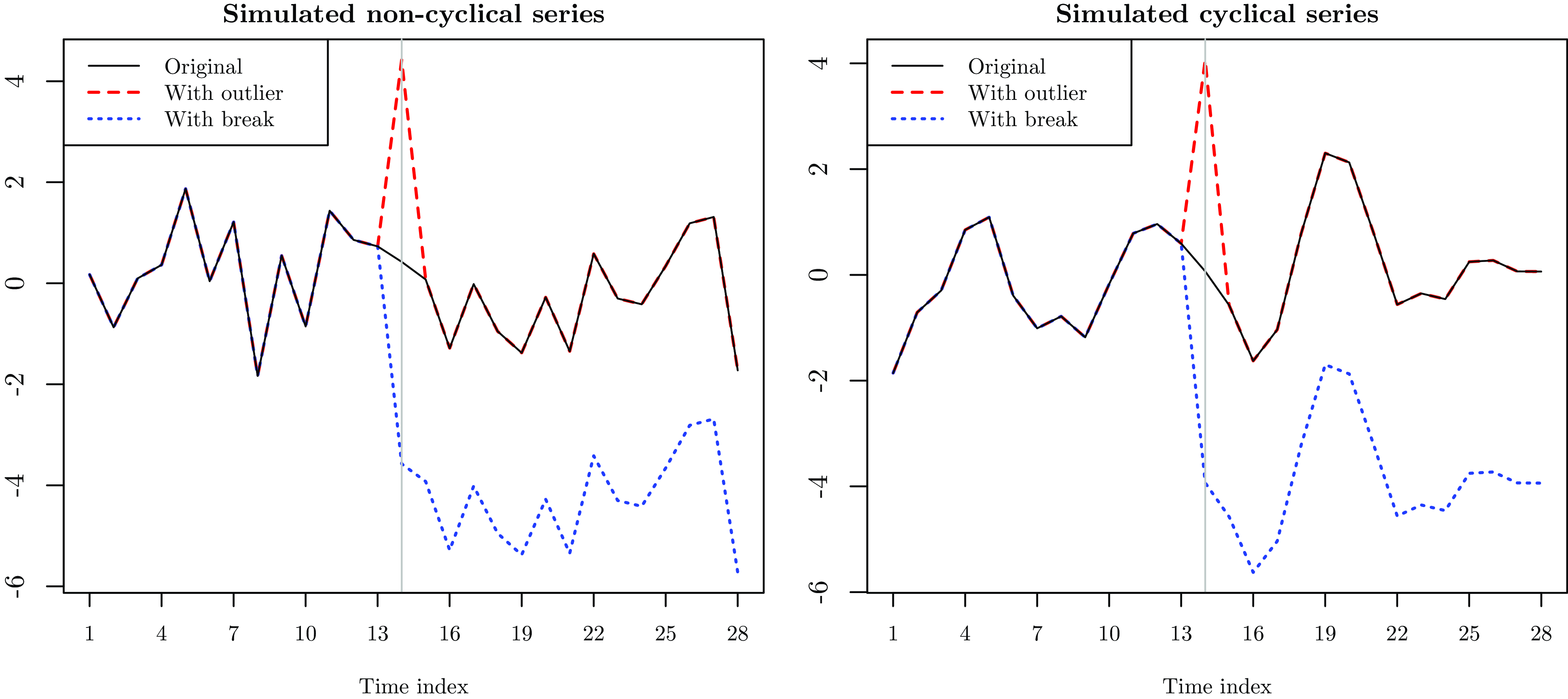
. Fig. 3 displays an example of the transformation for a non-cyclical and a cyclical time series from the data set
$\delta \in \{1,\ldots, 5\}$
. Fig. 3 displays an example of the transformation for a non-cyclical and a cyclical time series from the data set $\mathcal{S}_1$
.
$\mathcal{S}_1$
.
Cyclical and non-cyclical series with and without an outlier and a break. Notes: This figure displays two simulated paths from $\mathcal{S}_1$
, where one is non-cyclical and the other is cyclical. The original simulations are given by the straight black lines. The dashed red lines correspond to their transformation where an outlier with size
$\mathcal{S}_1$
, where one is non-cyclical and the other is cyclical. The original simulations are given by the straight black lines. The dashed red lines correspond to their transformation where an outlier with size $\delta =4$
occurs at time
$\delta =4$
occurs at time $s=14$
. The dotted blue lines correspond to the transformation where a structural break with size
$s=14$
. The dotted blue lines correspond to the transformation where a structural break with size $\delta =4$
occurs at time
$\delta =4$
occurs at time $s=14$
.
$s=14$
.
When the NN models are trained using data containing outliers or structural breaks, the training sets include series with $\delta \in \{0,1,2,3\}$
but not with
$\delta \in \{0,1,2,3\}$
but not with $\delta \in \{4,5\}$
. However, the testing data sets include series with all values of
$\delta \in \{4,5\}$
. However, the testing data sets include series with all values of $\delta$
, i.e.
$\delta$
, i.e. $\delta \in \{0,\ldots, 5\}$
. This allows us to determine how the NN models generalize their detection of cycles in the presence of outliers and breaks on which they were not trained, and in particular to
$\delta \in \{0,\ldots, 5\}$
. This allows us to determine how the NN models generalize their detection of cycles in the presence of outliers and breaks on which they were not trained, and in particular to $\delta =4$
or
$\delta =4$
or $5$
. In the remainder of this section, a data set
$5$
. In the remainder of this section, a data set $\mathcal{S}_i$
to which outliers and structural breaks were added is denoted by
$\mathcal{S}_i$
to which outliers and structural breaks were added is denoted by $\mathcal{S}_i^{\star }$
. The set
$\mathcal{S}_i^{\star }$
. The set $\mathcal{S}_i^{\star }$
includes a balanced mix of the original time series and the time series with either outliers or structural breaks at different times
$\mathcal{S}_i^{\star }$
includes a balanced mix of the original time series and the time series with either outliers or structural breaks at different times $s$
and different values of
$s$
and different values of $\delta \in \{0,1,2,3\}$
. Note that the data sets
$\delta \in \{0,1,2,3\}$
. Note that the data sets $\mathcal{S}_i^{\star }$
and
$\mathcal{S}_i^{\star }$
and $\mathcal{S}_j^{\star }$
for
$\mathcal{S}_j^{\star }$
for $i\neq j$
still differ in the length of the cycle period.
$i\neq j$
still differ in the length of the cycle period.
Figs. 4, 5, 6, and 7 display the performance measures with accuracy rates on the left columns, true positive rates on the middle columns, and true negative rates on the right columns. Figs. 4 and 5 focus on outliers, where the results in Fig. 4 are such that the NNs are trained on data without outliers, whereas in Fig. 5 the NNs are trained with outliers. Analogously, Figs. 6 and 7 focus on structural breaks, where the results in Fig. 6 are such that the NNs are trained on data without breaks, whereas in Fig. 7 the NNs are trained with breaks. In particular, the test data sets are $\mathcal{S}_j^{\star }$
,
$\mathcal{S}_j^{\star }$
, $j=1,\ldots, 5$
, and in Figs. 4 and 6 the NN models are trained on
$j=1,\ldots, 5$
, and in Figs. 4 and 6 the NN models are trained on $\cup _{1\leq i \leq 4}\mathcal{S}_i \setminus \mathcal{S}_j$
for
$\cup _{1\leq i \leq 4}\mathcal{S}_i \setminus \mathcal{S}_j$
for $j=1,\ldots, 4$
and
$j=1,\ldots, 4$
and $\cup _{1\leq i \leq 4}\mathcal{S}_i$
, respectively, whereas in Figs. 5 and 7 the NN models are trained on
$\cup _{1\leq i \leq 4}\mathcal{S}_i$
, respectively, whereas in Figs. 5 and 7 the NN models are trained on $\cup _{1\leq i \leq 4}\mathcal{S}_i^{\star } \setminus \mathcal{S}_j^{\star }$
for
$\cup _{1\leq i \leq 4}\mathcal{S}_i^{\star } \setminus \mathcal{S}_j^{\star }$
for $j=1,\ldots, 4$
and
$j=1,\ldots, 4$
and $\cup _{1\leq i \leq 4}\mathcal{S}_i^{\star }$
, respectively. The results are broken down by length of cycle periods in each row of the figures, i.e., the test data sets
$\cup _{1\leq i \leq 4}\mathcal{S}_i^{\star }$
, respectively. The results are broken down by length of cycle periods in each row of the figures, i.e., the test data sets $\mathcal{S}_j^{\star }$
for
$\mathcal{S}_j^{\star }$
for $j=1,\ldots, 5$
.
$j=1,\ldots, 5$
.
Accuracy, sensitivity, and specificity of all methodologies in the presence of outliers where the NN models are trained on data without outliers. Notes: This figure displays the accuracy rates (left columns), the true positive rates (middle columns) and the true negative rates (right columns) in function of the size of the outliers $\delta =0$
,
$\delta =0$
, $1$
,
$1$
, $2$
,
$2$
, $3$
,
$3$
, $4$
and
$4$
and $5$
for all methodologies on the test data
$5$
for all methodologies on the test data $\mathcal{S}_j^{\star }$
when the training data set is
$\mathcal{S}_j^{\star }$
when the training data set is $\cup _{1\leq i \leq 4}\mathcal{S}_i \setminus \mathcal{S}_j$
, for
$\cup _{1\leq i \leq 4}\mathcal{S}_i \setminus \mathcal{S}_j$
, for $j=1,2,3,4$
, as well as the performance on the test data
$j=1,2,3,4$
, as well as the performance on the test data $\mathcal{S}_5^{\star }$
when the training data set is
$\mathcal{S}_5^{\star }$
when the training data set is $\cup _{1\leq i \leq 4}\mathcal{S}_i$
, i.e. the training data sets do not contain outliers. The results from the autoregressive models and the
$\cup _{1\leq i \leq 4}\mathcal{S}_i$
, i.e. the training data sets do not contain outliers. The results from the autoregressive models and the $g$
-test with
$g$
-test with $p$
-value threshold
$p$
-value threshold $0.05$
with and without Bonferroni correction are given by the dashed lines. The results from the neural networks are given by the straight lines.
$0.05$
with and without Bonferroni correction are given by the dashed lines. The results from the neural networks are given by the straight lines.
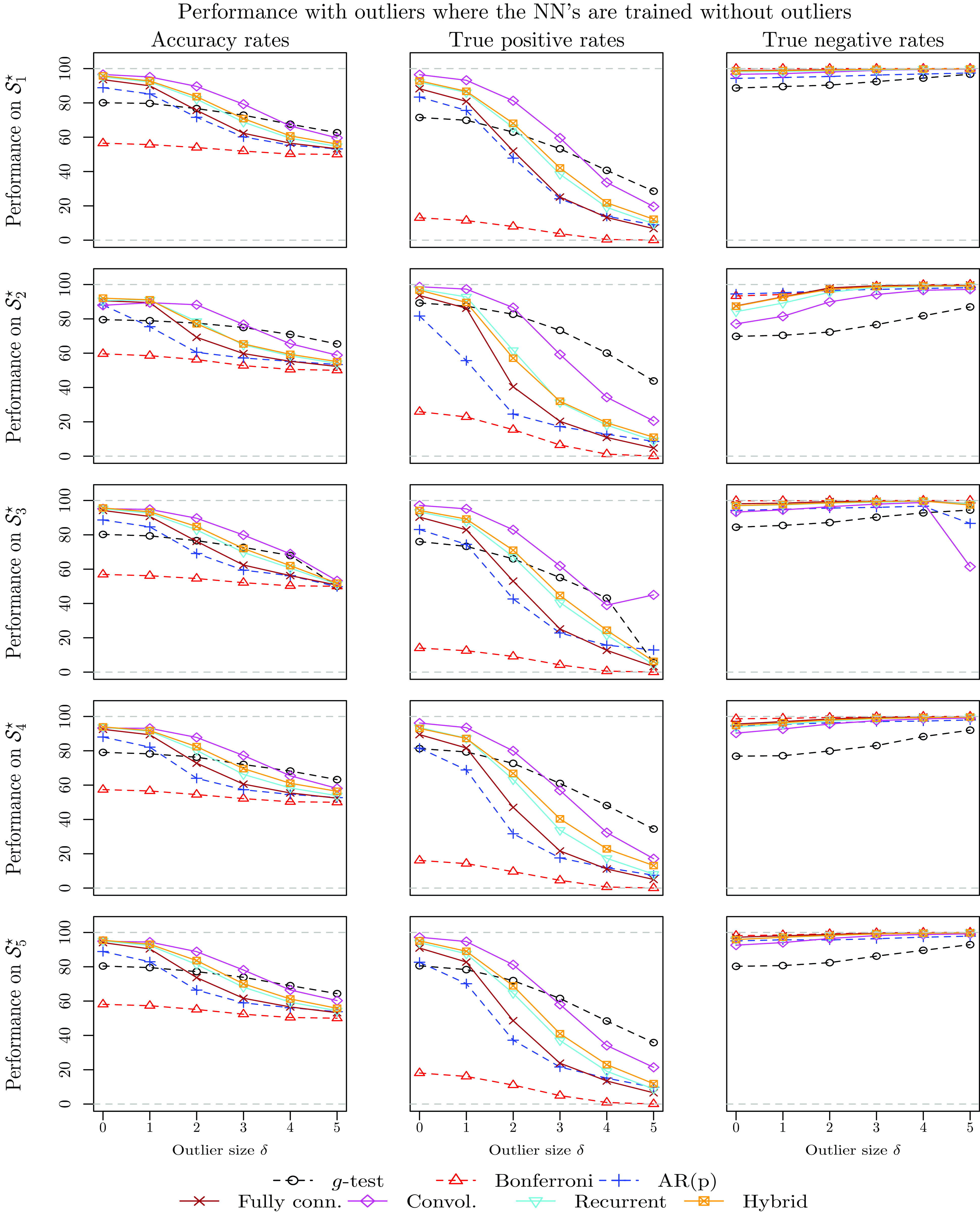
Accuracy, sensitivity, and specificity of all methodologies in the presence of outliers where the NN models are trained on data with outliers. Notes: This figure displays the accuracy rates (left columns), the true positive rates (middle columns), and the true negative rates (right columns) in function of the size of the outliers $\delta =0$
,
$\delta =0$
, $1$
,
$1$
, $2$
,
$2$
, $3$
,
$3$
, $4$
and
$4$
and $5$
for all methodologies on the test data
$5$
for all methodologies on the test data $\mathcal{S}_j^{\star }$
when the training data set is
$\mathcal{S}_j^{\star }$
when the training data set is $\cup _{1\leq i \leq 4}\mathcal{S}^{\star }_i \setminus \mathcal{S}^{\star }_j$
, for
$\cup _{1\leq i \leq 4}\mathcal{S}^{\star }_i \setminus \mathcal{S}^{\star }_j$
, for $j=1,2,3,4$
, as well as the performance on the test data
$j=1,2,3,4$
, as well as the performance on the test data $\mathcal{S}_5^{\star }$
when the training data set is
$\mathcal{S}_5^{\star }$
when the training data set is $\cup _{1\leq i \leq 4}\mathcal{S}_i^{\star }$
, i.e. the training data sets contain outliers. The results from the autoregressive models and the
$\cup _{1\leq i \leq 4}\mathcal{S}_i^{\star }$
, i.e. the training data sets contain outliers. The results from the autoregressive models and the $g$
-test with
$g$
-test with $p$
-value threshold
$p$
-value threshold $0.05$
with and without Bonferroni correction are given by the dashed lines. The results from the neural networks are given by the straight lines.
$0.05$
with and without Bonferroni correction are given by the dashed lines. The results from the neural networks are given by the straight lines.

Accuracy, sensitivity, and specificity of all methodologies in the presence of structural breaks in the mean where the NN models are trained on data without breaks. Notes: This figure displays the accuracy rates (left columns), the true positive rates (middle columns) and the true negative rates (right columns) in function of the size of the break $\delta =0$
,
$\delta =0$
, $1$
,
$1$
, $2$
,
$2$
, $3$
,
$3$
, $4$
and
$4$
and $5$
for all methodologies on the test data
$5$
for all methodologies on the test data $\mathcal{S}_j^{\star }$
when the training data set is
$\mathcal{S}_j^{\star }$
when the training data set is $\cup _{1\leq i \leq 4}\mathcal{S}_i \setminus \mathcal{S}_j$
, for
$\cup _{1\leq i \leq 4}\mathcal{S}_i \setminus \mathcal{S}_j$
, for $j=1,2,3,4$
, as well as the performance on the test data
$j=1,2,3,4$
, as well as the performance on the test data $\mathcal{S}_5^{\star }$
when the training data set is
$\mathcal{S}_5^{\star }$
when the training data set is $\cup _{1\leq i \leq 4}\mathcal{S}_i$
, i.e. the training data sets do not contain breaks. The results from the autoregressive models and the
$\cup _{1\leq i \leq 4}\mathcal{S}_i$
, i.e. the training data sets do not contain breaks. The results from the autoregressive models and the $g$
-test with
$g$
-test with $p$
-value threshold
$p$
-value threshold $0.05$
with and without Bonferroni correction are given by the dashed lines. The results from the neural networks are given by the straight lines.
$0.05$
with and without Bonferroni correction are given by the dashed lines. The results from the neural networks are given by the straight lines.
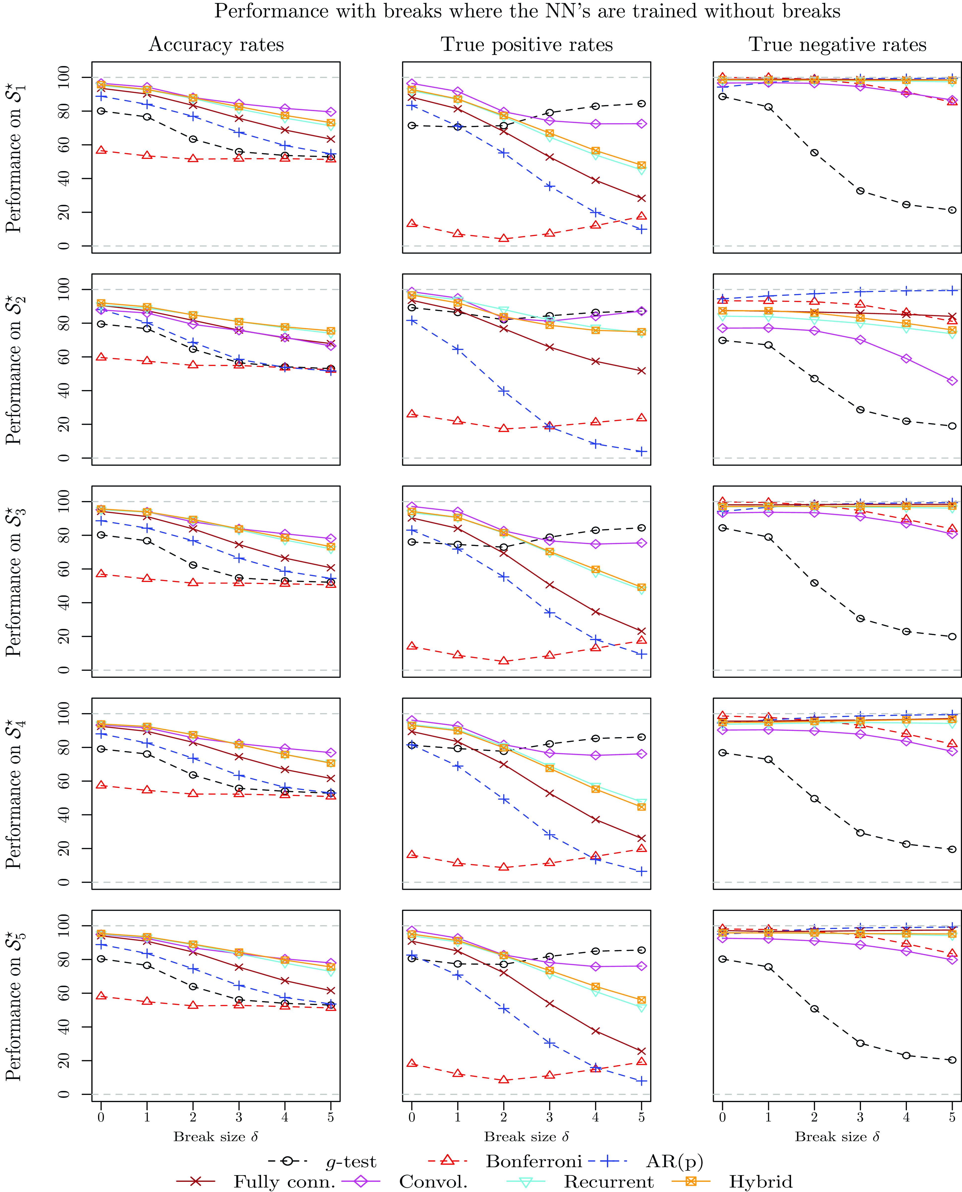
Accuracy, sensitivity, and specificity of all methodologies in the presence of structural breaks in the mean where the NN models are trained on data with breaks. Notes: This figure displays the accuracy rates (left columns), the true positive rates (middle columns), and the true negative rates (right columns) in function of the size of the break $\delta =0$
,
$\delta =0$
, $1$
,
$1$
, $2$
,
$2$
, $3$
,
$3$
, $4$
and
$4$
and $5$
for all methodologies on the test data
$5$
for all methodologies on the test data $\mathcal{S}_j^{\star }$
when the training data set is
$\mathcal{S}_j^{\star }$
when the training data set is $\cup _{1\leq i \leq 4}\mathcal{S}_i^{\star } \setminus \mathcal{S}_j^{\star }$
, for
$\cup _{1\leq i \leq 4}\mathcal{S}_i^{\star } \setminus \mathcal{S}_j^{\star }$
, for $j=1,2,3,4$
, as well as the performance on the test data
$j=1,2,3,4$
, as well as the performance on the test data $\mathcal{S}_5^{\star }$
when the training data set is
$\mathcal{S}_5^{\star }$
when the training data set is $\cup _{1\leq i \leq 4}\mathcal{S}_i^{\star }$
, i.e. the training data sets contain breaks. The results from the autoregressive models and the
$\cup _{1\leq i \leq 4}\mathcal{S}_i^{\star }$
, i.e. the training data sets contain breaks. The results from the autoregressive models and the $g$
-test with
$g$
-test with $p$
-value threshold
$p$
-value threshold $0.05$
with and without Bonferroni correction are given by the dashed lines. The results from the neural networks are given by the straight lines.
$0.05$
with and without Bonferroni correction are given by the dashed lines. The results from the neural networks are given by the straight lines.
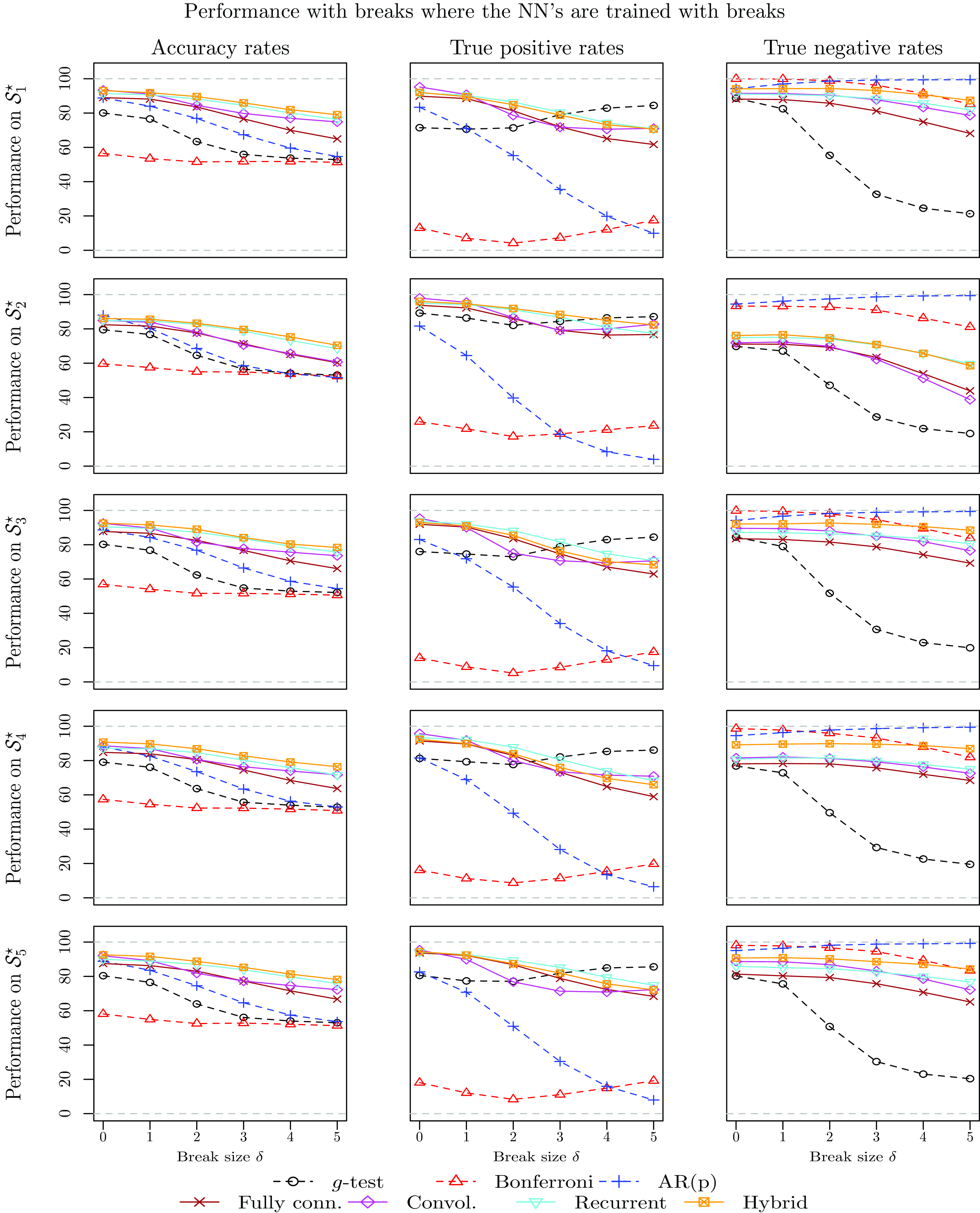
The left columns of Fig. 4 show that the performance of all methodologies deteriorates with the size of the outliers in all test data sets. The accuracy rate of the AR(p) models falls quickly at $\delta =2$
below that of the uncorrected
$\delta =2$
below that of the uncorrected $g$
-test. Interestingly, the
$g$
-test. Interestingly, the $g$
-test without Bonferroni correction is the least impacted by the size of the outlier except on the test data
$g$
-test without Bonferroni correction is the least impacted by the size of the outlier except on the test data $\mathcal{S}_3^{\star }$
. In particular, in most cases, the
$\mathcal{S}_3^{\star }$
. In particular, in most cases, the $g$
-test gives the highest accuracy rate from
$g$
-test gives the highest accuracy rate from $\delta =4$
. Among the NN models, the architecture that is most robust to outliers is the convolutional NN, which has an accuracy rate consistently above that of the other architectures. However, as with all other methods except the uncorrected
$\delta =4$
. Among the NN models, the architecture that is most robust to outliers is the convolutional NN, which has an accuracy rate consistently above that of the other architectures. However, as with all other methods except the uncorrected $g$
-test, its accuracy rate drops near 60% for large outliers. From the middle and right columns of Fig. 4, the deterioration of the performance of all models appears to be due to a high rejection rate of cyclicality leading to poor true positive rates, while true negative rates are close to 100%. Shifting now the focus towards Fig. 5, it turns out that training the NN models on data with outliers significantly improves their performance, except for
$g$
-test, its accuracy rate drops near 60% for large outliers. From the middle and right columns of Fig. 4, the deterioration of the performance of all models appears to be due to a high rejection rate of cyclicality leading to poor true positive rates, while true negative rates are close to 100%. Shifting now the focus towards Fig. 5, it turns out that training the NN models on data with outliers significantly improves their performance, except for $\delta =5$
on the test data
$\delta =5$
on the test data $\mathcal{S}_3^{\star }$
. Discounting that exception, the accuracy rates of the convolutional, the recurrent, and the hybrid architectures retain levels of accuracy close to their levels without outliers (i.e.
$\mathcal{S}_3^{\star }$
. Discounting that exception, the accuracy rates of the convolutional, the recurrent, and the hybrid architectures retain levels of accuracy close to their levels without outliers (i.e. $\delta =0$
). However, the accuracy rates of the fully connected NN architecture fall towards those of the uncorrected
$\delta =0$
). However, the accuracy rates of the fully connected NN architecture fall towards those of the uncorrected $g$
-test despite being trained on data with outliers. Overall, the figures suggest that once trained on data containing series with outliers, the top-performing model is the hybrid NN, closely followed by the convolutional or the recurrent models. The methodologies based on the FNN, AR(p), and the
$g$
-test despite being trained on data with outliers. Overall, the figures suggest that once trained on data containing series with outliers, the top-performing model is the hybrid NN, closely followed by the convolutional or the recurrent models. The methodologies based on the FNN, AR(p), and the $g$
-test are too sensitive to the presence of outliers compared to the CNN, RNN, and the hybrid NN.
$g$
-test are too sensitive to the presence of outliers compared to the CNN, RNN, and the hybrid NN.
The left columns on Fig. 6 show that the accuracy rates of all models are also decreasing with the size of the structural break. Nevertheless, the figure suggests that the accuracy rates of NN models are less sensitive to the presence of structural breaks than outliers, with the exception of the fully connected NN whose accuracy rates fall near those of the AR(p) and the $g$
-test. The reasonable performance of the convolutional, the recurrent, and the hybrid architectures seems to be associated with a mild decrease in the true positive rate compared to the case with outliers. Furthermore, Fig. 7 shows that training the NN models on data containing structural breaks improves their accuracy rate and the true positive rates, but the improvement is less noticeable than in the case of data with outliers. Where the NN models are trained with data that include structural breaks (i.e. Fig. 7), the top-performing model is again the hybrid architecture.
$g$
-test. The reasonable performance of the convolutional, the recurrent, and the hybrid architectures seems to be associated with a mild decrease in the true positive rate compared to the case with outliers. Furthermore, Fig. 7 shows that training the NN models on data containing structural breaks improves their accuracy rate and the true positive rates, but the improvement is less noticeable than in the case of data with outliers. Where the NN models are trained with data that include structural breaks (i.e. Fig. 7), the top-performing model is again the hybrid architecture.
The superior performance of NN models in the presence of outliers and structural breaks can be attributed to their ability to learn from diverse training data and extract underlying patterns rather than relying on parametric assumptions. Traditional AR models estimate coefficients that are directly impacted by sudden changes in the mean or extreme observations, leading to instability in cycle classification. In contrast, NN architectures learn representations that emphasize recurrent patterns while de-emphasizing transient distortions. By training NN models on both “clean” and “perturbed” series, they develop robustness to irregularities that would otherwise bias AR-based detection methods.
Overall, the analysis suggests that for a training data set without outliers, the hybrid architecture outperforms all other models when there are no outliers or structural breaks, but that performance is sensitive to the presence of such features, and the least sensitive architecture is the convolutional NN. However, once trained on data that contain outliers or structural breaks, the hybrid architecture is to be preferred. The methodologies based on AR(p) or the $g$
-test are too sensitive to the presence of outliers and structural breaks, and their performance deteriorates with the size of the outlier and the break, especially for the AR(p). Of course, it is worth noting that the performance of the AR(p) and
$g$
-test are too sensitive to the presence of outliers and structural breaks, and their performance deteriorates with the size of the outlier and the break, especially for the AR(p). Of course, it is worth noting that the performance of the AR(p) and $g$
-test could possibly be improved using an appropriate method to correct the time series for the outliers and structural breaks. Such corrections were not used here as they are not common in the literature on the underwriting cycle.
$g$
-test could possibly be improved using an appropriate method to correct the time series for the outliers and structural breaks. Such corrections were not used here as they are not common in the literature on the underwriting cycle.
5. Empirical study
This section reports the results of the classification of the AUTOSEG data of prices. Recall that based on the simulation study in the previous section, the NN models stand out as the most accurate on the test data for cycle detection, especially the hybrid architecture trained on data with outliers or structural breaks in the means. Nevertheless, for the sake of completeness, this section reports the classification outcome of all methods. Note that in this section, the NN models were trained using all simulated data, namely either on $\cup _{1\leq i\leq 5}\mathcal{S}_i$
for the models trained on data without outliers and breaks, or on
$\cup _{1\leq i\leq 5}\mathcal{S}_i$
for the models trained on data without outliers and breaks, or on $\cup _{1\leq i\leq 5}\mathcal{S}_i^{\star }$
for the models trained on data with outliers and breaks.
$\cup _{1\leq i\leq 5}\mathcal{S}_i^{\star }$
for the models trained on data with outliers and breaks.
The classification outcome from all methods is reported in Table 3, containing the proportions of price time series classified as cyclical in the middle column, where the classification is performed per risk profile, as well as the classification outcome at the aggregate level in the right column, using average market price across all risk profiles weighted by the exposure.
Analysis of price cycles
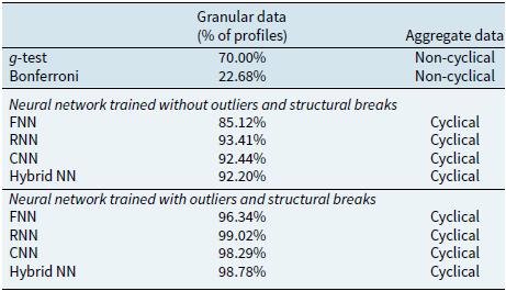
Notes: The middle column of this table reports the proportion of cyclical time series of prices from the classification of all models. The right column reports the outcome of the classification of all models for the data aggregated at the market level, i.e. the average market price where the average is weighted by the exposure. The neural network models were trained using either all simulated data $\cup _{1\leq i\leq 5}\mathcal{S}_i$
without outliers and structural breaks or all simulated data
$\cup _{1\leq i\leq 5}\mathcal{S}_i$
without outliers and structural breaks or all simulated data $\cup _{1\leq i\leq 5}\mathcal{S}_i^{\star }$
with outliers and structural breaks.
$\cup _{1\leq i\leq 5}\mathcal{S}_i^{\star }$
with outliers and structural breaks.
The findings provide strong evidence that insurance prices for almost all risk profiles exhibit cyclical behavior. The AR(p) methodology typically used in the literature detects cyclicality in 79.51% of risk profiles, while the $g$
-test without correction detects it in 70%. The
$g$
-test without correction detects it in 70%. The $g$
-test with Bonferroni correction detects cyclicality in 20.68%, but as demonstrated in the simulation study, this correction leads to over-rejection of cyclicality. The NN models identify cyclicality in proportions exceeding 90%, with the hybrid architecture trained on data with outliers and breaks (i.e. the top-performing model in the simulation study) detecting cyclicality in 98.78% of the time series, or 405 out of 410 risk profiles. The classification of aggregate prices is consistent with that of the granular data, where all methodologies classify the average market price as cyclical, except for the
$g$
-test with Bonferroni correction detects cyclicality in 20.68%, but as demonstrated in the simulation study, this correction leads to over-rejection of cyclicality. The NN models identify cyclicality in proportions exceeding 90%, with the hybrid architecture trained on data with outliers and breaks (i.e. the top-performing model in the simulation study) detecting cyclicality in 98.78% of the time series, or 405 out of 410 risk profiles. The classification of aggregate prices is consistent with that of the granular data, where all methodologies classify the average market price as cyclical, except for the $g$
-tests. To the best of my knowledge, this is the first paper that provides evidence of cyclicality in insurance prices, and at this level of granularity.
$g$
-tests. To the best of my knowledge, this is the first paper that provides evidence of cyclicality in insurance prices, and at this level of granularity.
The interpretation of the above results can be subject to two important criticisms.
The first one is that, strictly speaking, the NN models employed in this paper are trained to distinguish between cyclical AR(2) and cosine-based series from AR(1)/AR(0), and do not necessarily identify all types of cyclicality. The simulation study, although comprehensive in the treatment of the standard processes considered in the literature, does not investigate how NN models would classify series with complex but not cyclical temporal structure. In particular, the simulation study in Section 4 does not address the performance of NNs trained on noisy sinusoids and AR(p) with $p\leq 2$
when the series to be classified are e.g. non-cyclical AR(3) models, heteroscedastic, and/or exhibiting both outliers and structural breaks. Nevertheless, the preliminary tests performed on the data suggest absence of heteroscedasticity, and i.i.d. residuals when the series are modeled using AR(1) or AR(2) models. In a separate analysis, an AR(3) was estimated for all series, but it outperforms the AR(1) and AR(2) in only a few instances, namely for 20 series of price. For all these series, the condition of AR(3) cyclicality was investigated numerically by verifying whether the characteristic equation of the process has a pair of complex roots, and both AR(3) and AR(2) suggest cyclicality.
$p\leq 2$
when the series to be classified are e.g. non-cyclical AR(3) models, heteroscedastic, and/or exhibiting both outliers and structural breaks. Nevertheless, the preliminary tests performed on the data suggest absence of heteroscedasticity, and i.i.d. residuals when the series are modeled using AR(1) or AR(2) models. In a separate analysis, an AR(3) was estimated for all series, but it outperforms the AR(1) and AR(2) in only a few instances, namely for 20 series of price. For all these series, the condition of AR(3) cyclicality was investigated numerically by verifying whether the characteristic equation of the process has a pair of complex roots, and both AR(3) and AR(2) suggest cyclicality.
The second criticism of this study is that the data set encompasses only 14 years (approximately 3 cycles based on the estimation of the AR(2) on aggregate premiums), making it challenging to identify cyclicality from an econometric perspective. However, the simulation study demonstrates that NNs were able to detect cyclical AR(2) patterns and noisy sinusoids across various cycle lengths with the same number of observations as the empirical study. Therefore, based on the simulation study results, the number of observations in the empirical analysis is not a significant concern.
6. Conclusion
The present paper addresses the methodological issue of cycle detection in the insurance industry using NNs. The efficacy of NNs is demonstrated on simulated data and compared to that of traditional methods. The simulation study highlights the performance of NN models in cycle detection under various settings, including when the data contain outliers and structural breaks. The NN-based methodology is then applied to a novel granular data set from the Brazilian insurance industry of prices per risk profile. The application shows that, despite the skepticism expressed in the literature, insurance cycles exist, and they manifest themselves in prices of almost all risk profiles.
While this study focuses on NNs, other machine learning techniques, such as gradient boosting, could also be considered for cycle detection. Tree-based methods have shown strong classification performance in various applications and could, therefore, also perform well in contexts where temporal dependencies in time series have to be taken into account. Nevertheless, NN architectures, particularly convolutional and recurrent models, are designed to capture sequential patterns, making them well-suited for this task. Future research could explore the performance of alternative machine learning methods, but the findings presented here highlight the advantages of NNs in cycle detection.
The results of this study raise several avenues for future research. First, the high classification accuracy of NNs suggests that they could be adapted to detect other time-series characteristics, such as stationarity, autocorrelation, or seasonality. Extending the current methodology to a broader set of time-series properties could provide further insights into insurance market dynamics, and it would also be relevant more generally in the context of time-series analysis. Second, a natural extension is to develop methods for identifying cycle peaks and troughs, which could assist actuaries in designing more responsive pricing strategies. This could involve integrating NN-based cycle detection with change-point detection techniques or state-space models. Third, Fig. 1 suggests that insurance prices for different risk profiles exhibit a degree of synchronization. Future research could investigate whether this synchronicity is driven by common macroeconomic factors, regulatory changes, or market competition. This could be explored using multivariate models or causal inference techniques to better understand the interdependencies between risk profiles.
Data availability statement
The code that supports the findings of this study is available on request from the author. The data source is provided in the main text.
Funding statement
This work was supported by Fundación MAPFRE, grant Ignacio H. de Larramendi for insurance and social protection.
Competing interests
The author declares none.


 Open access