


1 Introduction
In the past, psychological research has traditionally emphasized questionnaire assessments, often overlooking the study of actual behavior (Funder, Reference Funder2009). While investigating behavior in the field was previously challenging due to factors like high costs, time constraints, and intrusiveness (Baumeister et al., Reference Baumeister, Vohs and Funder2007), it is now facilitated by the rise of digital devices. Using off-the-shelf electronics such as smartphones and smartwatches, researchers can automatically gather behavioral (and situational) data from people’s everyday lives through mobile sensing. More specifically, mobile sensing enables the passive collection of data from system logs and native sensors present in these devices via designated research apps (for an introduction to the method, see Mehl et al., Reference Mehl, Eid, Wrzus, Harari, Ebner-Priemer and Insel2024). These sensing apps can be installed on participants’ own devices, making data collection less intrusive and more financially economical and environmentally friendly compared to predecessors like portable cameras or audio recorders (Miller, Reference Miller2012; Schoedel & Mehl, Reference Schoedel, Mehl, Reis, West and Judd2024). As a result, sensing data can be collected over extended periods in longitudinal study designs.
For a long time, mobile sensing has primarily been implemented on smartphones, as these devices are widespread in the Western world (GSMA, 2025) and are with their users most of the time (Dey et al., Reference Dey, Wac, Ferreira, Tassini, Hong and Ramos2011). While smartwatches and other wearables are now becoming increasingly important—especially for collecting physiological and movement-related data (Fuller et al., Reference Fuller, Colwell, Low, Orychock, Tobin, Simango, Buote, Van Heerden, Luan, Cullen, Logan Slade and Taylor2020; Wac, Reference Wac2018)—smartphones still play a central role in mobile-sensing research. Their ability to combine passive sensing with active data collection through ecological momentary assessments (EMAs; Wrzus & Neubauer, Reference Wrzus and Neubauer2023) makes them especially useful for capturing behavioral data alongside participants’ momentary subjective experiences (Conner & Mehl, Reference Conner, Mehl and Kosslyn2015).
Drawing on the unprecedented accessibility and variety of behavioral data collected from smartphones or other sensing devices, researchers have started to explore a range of psychological phenomena in everyday life, for example, personality traits (Stachl, Au, et al., Reference Stachl, Au, Schoedel, Gosling, Harari, Buschek, Völkel, Schuwerk, Oldemeier, Ullmann, Hussmann, Bischl and Bühner2020), sociability (Harari, Müller, et al., Reference Harari, Müller, Stachl, Wang, Wang, Bühner, Rentfrow, Campbell and Gosling2020), mood states (Spathis et al., Reference Spathis, Servia-Rodriguez, Farrahi, Mascolo and Rentfrow2019), chronotype (Schoedel et al., Reference Schoedel, Pargent, Au, Völkel, Schuwerk, Bühner and Stachl2020), and symptoms of depression and anxiety (Moshe et al., Reference Moshe, Terhorst, Opoku Asare, Sander, Ferreira, Baumeister, Mohr and Pulkki-Råback2021). Thereby, new terms have emerged to describe this line of research, including Psychoinformatics in psychometrics (Markowetz et al., Reference Markowetz, Błaszkiewicz, Montag, Switala and Schlaepfer2014), Personality Sensing in the differential context (Harari, Vaid, et al., Reference Harari, Vaid, Müller, Stachl, Marrero, Schoedel, Bühner and Gosling2020), and Digital Phenotyping in mental health research (Insel, Reference Insel2017).
While mobile sensing holds great promise for providing valuable insights from everyday life into psychological phenomena, it also poses considerable methodological challenges that researchers must overcome. The data generated by sensing apps are highly complex (i.e., timestamped event data), arrive in large volumes (i.e., dozens of events per second), and encompass various modalities (e.g., usage logs, text data, and GPS coordinates). Furthermore, they often contain inconsistencies due to logging errors or discrepancies between devices. Consequently, unlike item responses from self-report questionnaires, these high-dimensional data require extensive preprocessing efforts to derive meaningful behavioral variables that are suitable for studying the phenomena of interest. However, most psychologists lack training in handling mobile-sensing data and are often left without methodological guidance (Wrzus & Schoedel, Reference Wrzus and Schoedel2023). As a result, the field often relies on conventional analysis strategies. These approaches could be complemented by emerging methods that allow researchers to more fully leverage the rich potential of these data and thereby enhance both theoretical and empirical insights.
To advance mobile-sensing research, we begin by summarizing the current state of data processing and then present three use cases that go beyond current practices to demonstrate more advanced methods. For this purpose, we use app usage logs as an exemplary starting point for extracting behavioral variables. We systematically report our preprocessing efforts, focusing on two key dimensions: data enrichment, which reflects the extend to which raw sensing data are combined with contextual information, and data aggregation, which captures how variables are summarized across individual data points.
2 Data collection
To illustrate our preprocessing pipelines and use cases, we use an exemplary dataset collected in the Smartphone Sensing Panel Study (SSPS; Schoedel & Oldemeier, Reference Schoedel and Oldemeier2020). This study was part of the interdisciplinary PhoneStudy research project at LMU Munich and was conducted in collaboration with the Leibniz Institute for Psychology (ZPID). The aim of the SSPS was to create a benchmark dataset for the research community, comprising longitudinal and high-dimensional sensing data, along with self-report data about a wide range of psychological phenomena. The data collection was comprised of mobile sensing, EMAs, and online surveys, but here, we mostly concentrate our report on the unique sensing data. Additional procedures can be found in our preregistered study protocol (Schoedel & Oldemeier, Reference Schoedel and Oldemeier2020) and initial publications by große Deters and Schoedel (Reference große Deters and Schoedel2024), Reiter and Schoedel (Reference Reiter and Schoedel2024), and Schoedel et al. (Reference Schoedel, Kunz, Bergmann, Bemmann, Bühner and Sust2023).
2.1 Transparency and openness statement
All procedures of the SSPS received approval from the responsible ethics committee at LMU Munich and complied with the General Data Protection Regulation (GDPR). Before data collection, all participants provided their informed consent, which they could withdraw at any point during the study without giving a reason.
The analyses presented in this manuscript are purely exploratory and only serve illustrative purposes for the preprocessing pipelines proposed here. We also provide an OSF repository with our online supplemental materials (OSMs) and the code for data preprocessing and analysis. All analyses were conducted in the statistical software R (version 4.2.1 for the basic preprocessing and data enrichment steps; version 4.4.1 for data aggregation steps; R Core Team, 2024). For reproducibility purposes, we utilized the package management tool groundhog (Simonsohn & Gruson, Reference Simonsohn and Gruson2024). While the data privacy prevents us from sharing the raw sensing data, we provide the set of aggregated variables extracted here in our repository.
2.2 Study procedures
The SSPS took place between May and November 2020 for either three or six months, depending on random group assignment. All data were collected using our custom research app, PhoneStudy, which participants installed on their personal smartphones at study onset. Subsequently, the app began to continuously log various mobile-sensing data (see the next section). In addition, the app administered—depending on the group assignment—three to six monthly online surveys (approx. 30 minutes) and one or two 14-day EMA waves, collecting self-reports on various psychological constructs (see Schoedel & Oldemeier, Reference Schoedel and Oldemeier2020 for an overview of instruments).
The total sample of the SSPS comprised data from 850 participants, collected according to quotas that represented the German population in terms of age, gender, education, income, religion, and relationship status in 2020. Only persons between 18 and 65 years could participate. Furthermore, participants had been required to be the sole users of a smartphone running on the Android operating system (version 5 or higher) due to technical reasons.
In this manuscript, we used only a fraction of the complete data set, specifically the demographics from the first survey (May 2020), as well as the sensing data collected during the first and second EMA waves (07/27/2020–08/09/2020; 09/21/2020–10/04/2020) and the corresponding EMAs (situation perception and sleep diary). We only included participants with at least three sensing days and who answered at least 10 EMAs in wave 1. These components of the SSPS exhibited a sample size of N = 538, from which 473 participants provided their demographic information: ages ranged from 18 to 65, with an average of 41 years (SD = 12.6). Additionally, 45.7% (n = 216) of participants identified as female, while 54.3% identified as male (n = 257).
2.3 Data structure
The PhoneStudy app continuously collected data from participants’ personal smartphones and spanned 13 distinct sensing modalities, including screen status, notifications, usage logs (for phone, apps, keyboard, and music player), connectivity reports (power and headphone plug, WiFi, Bluetooth, and flight mode), and sensor data (GPS and physical activity). Data were logged as timestamped entries and, depending on the sensing modality, stored with varying specifications (see Table 1). Beyond sensing, the app administered EMAs and stored the corresponding self-reports and their timestamps in a separate table.
Exemplary logs of screen status, app usage, and GPS sensors

Table 1 Long description
The table contains seven columns: Timestamp, Activity, Event, Name, Package name, Latitude, and Longitude.
* The log begins at 2020-07-27 21:40:02 with a G P S activity at latitude 48.150509 and longitude 11.580299.
* At 21:50:07, the screen status changes to O N underscore L O C K E D, followed by a second G P S log at 21:50:09 (latitude 48.155722, longitude 11.582963).
* At 21:50:11, the screen is O N underscore U N L O C K E D.
* From 21:50:13 to 21:53:55, multiple A P P S activities are logged for Facebook (com dot facebook dot katana), showing a sequence of activity resumed, paused, and finally stopped.
* At 21:53:50, a brief background process for com dot android dot pacprocessor occurs.
* At 21:53:51, B B C news (bbc dot mobile dot news dot w w) resumes, then pauses at 21:57:40.
* At 21:57:41, the screen status is O F F underscore L O C K E D.
* A later G P S log at 22:20:02 shows the same coordinates as the 21:50:09 entry.
* The log concludes at 23:45:12 with WhatsApp (com dot whatsapp) resuming after the screen was unlocked at 23:45:09.
Note: Timestamp sorted logs of screen status, app usage, and GPS location from an Android smartphone, collected with the PhoneStudy mobile-sensing app. This is artificially generated data that has been simplified for illustrative purposes (e.g., removal of other recording modalities and adjustment of variable values).
To illustrate different cases of sensing data analysis, we will concentrate on the app usage logs, which provide rich behavioral information and allow for extracting variables at different levels of granularity (Sust, Talaifar, et al., Reference Sust, Talaifar, Stachl, Mehl, Eid, Wrzus, Harari and Ebner-Priemer2023). In addition, to further contextualize app usage, we will incorporate data from GPS sensors as well as self-report data from EMAs. We describe these sensing modalities in more detail below, but refrain from reporting on any other modalities and refer interested readers to the methods section of Schoedel et al. (Reference Schoedel, Kunz, Bergmann, Bemmann, Bühner and Sust2023).
2.3.1 App usage logs
App usage was logged in an event-based manner, meaning the PhoneStudy app captured data points whenever they occurred, specifically, whenever an app was used. The resulting logsFootnote 1 contain timestamped information regarding the package names of the used apps and event types (see Table 1). Package names serve as unique identifiers for each app (e.g., com.facebook.katana for Facebook or bbc.mobile.news.ww for BBC News) on distribution platforms such as the Google Play Store or on the devices where they are installed. Event types are defined by Android’s accessibility services (see Parry & Toth, Reference Parry and Toth2025 for a complete documentation) and encompass a variety of actions, including launch (type 1: activity resumed), transition to background (type 2: activity paused), or closure (type 23: activity stopped). As illustrated in Table 1, using a single app—for instance, opening, navigating within, and then closing the app Facebook—produces a sequence of recorded app events. Below, we discuss how these raw logs can be aggregated to behavioral variables on app usage.
2.3.2 GPS sensor data
GPS sensor data were logged via three different logging modes to provide an accurate representation of the user’s environment while conserving battery life. In particular, they were logged (a) at fixed intervals (e.g., every 10–60 minutes, depending on the smartphone model), (b) based on changes (i.e., whenever the coordinates altered significantly) using the Google Fence application programming interface (API), and (c) at the precise moment when EMAs were opened using the Google Snapshot API. The resulting sensing logs contain timestamped GPS coordinates, specifying (among other parameters) the latitude and longitude through the Fused Location Provider API (see Table 1). In Section 4.1, we use these data to provide context for app usage and present one (out of many possible) approaches to preprocess mobile-sensed GPS coordinates.
2.3.3 EMA data
EMAs were scheduled in a pseudo-randomized manner, with two to four questionnaires presented in one of four equally sized sections of the day (from 7 a.m. to 10 p.m. on weekdays and from 9 a.m. to 11 p.m. on weekends), while ensuring a minimum of 60 minutes between samplings. Questionnaires were prompted via a notification as soon as participants first used their smartphones actively after the scheduled time, to avoid provoking artificial smartphone usage (van Berkel et al., Reference van Berkel, Goncalves, Lovén, Ferreira, Hosio and Kostakos2019). The EMAs contained a varying number of short questions about participants’ current mood and situation, as well as sleep-related questions (only in the first EMA per day). While analyzing stand-alone EMA data falls outside the scope of our manuscript, these data are often combined with mobile-sensing data to connect subjective experiences with objective behavioral or situational information at the momentary level (e.g., Elmer et al., Reference Elmer, Fernández, Stadel, Kas and Langener2025; Schoedel et al., Reference Schoedel, Kunz, Bergmann, Bemmann, Bühner and Sust2023). Hence, we will incorporate EMA data into our preprocessing pipelines in Sections 4.2 and 4.3.
3 State-of-the-art preprocessing
Building on the app usage logs, we now explore current approaches to extracting variables from mobile-sensing data. We begin by introducing basic preprocessing steps and then review the current state of the art—that is, the methods most commonly used by researchers to analyze such data to date (see Parry & Toth, Reference Parry and Toth2025).
3.1 Data cleaning and preparation
The event sequences in Table 1 reveal several issues related to the sensing of app usage events, which we needed to consider before getting into further preprocessing. Specifically, app usage events usually exhibit ambiguous patterns, particularly due to multiple launch events (type 1) being recorded within one sequence when users navigate within the components (e.g., menu levels) of an app (Parry & Toth, Reference Parry and Toth2025). When counting the Facebook app launches in Table 1, it may appear as if the app was used three times instead of only once. Furthermore, there are often delays when logging closure events (type 23) after the app has not been actively used for a while (Parry & Toth, Reference Parry and Toth2025). At first glance, the raw sensing data in Table 1 may imply that the app Facebook is being closed at 21:53:55, even though the user started engaging with another app a few seconds prior. The complexity of these logging sequences is further exacerbated by system apps (e.g., com.android.pacprocessor), which generate logs without active user interaction through background processes like battery optimization tasks or network management (see also Parry & Toth, Reference Parry and Toth2025; Schoedel et al., Reference Schoedel, Oldemeier, Bonauer and Sust2022). Because of these ambiguous patterns, it is not possible to extract app usage variables by simply counting certain event types without some initial data cleaning.
Instead, it is essential first to define consecutive app usage sessions and to label the data patterns corresponding to one session. Only after this basic cleaning procedure can we derive meaningful variables on app usage behaviors. Here, as a first step, we removed app events created by system apps that are not produced through active user engagement and may have occurred during the usage session of a proper app. Then, consistent with standard practices in mobile-sensing research (Parry & Toth, Reference Parry and Toth2025), we defined the start time of an usage session as the first event when an app A was launched (type 1) and the end time as the app’s last logging event, before the launch of another app B (type 1) or the screen turning off. To implement this rationale, we developed a rule-based function to detect and label smartphone usage patterns within the dataset. This function first labeled all app events that occurred within the same smartphone usage session, that is, between the onset and offset of the phone’s screen, and assigned them a unique identifier. Within each smartphone session, the function then labeled all app events that occurred within the same app usage session, that is, between the launch (type 1) of an app A and either the launch of another app B (type 1) or the end of the smartphone usage session. Again, all events belonging to one app usage session obtained a unique identifier. Finally, based on these labeled data, we grouped the raw logs by unique app usage session identifier. We generated a new summary table with one entry per app usage session, stating its start and end times and the corresponding package name. This new table of app usage events then served as the starting point for all further preprocessing steps outlined below (see Table 2).
Summary table of individual app usage sessions after basic preprocessing of app usage logs

Table 2 Long description
The table contains nine columns: I D, Package name, Start, End, Duration, App category, Location category, E M A I D, and Bedtime I D.
* I D 34: com dot google dot android dot apps dot maps, 2020-07-27 19:00:42 to 19:05:14, duration 4.53, Orientation, Not at home.
* I D 35: com dot whatsapp, 2020-07-27 19:05:15 to 19:08:13, duration 2.97, Communication, Not at home.
* I D 36: com dot whatsapp, 2020-07-27 20:11:23 to 20:14:44, duration 3.35, Communication, Not at home, Bedtime I D 12.
* I D 37: com dot facebook dot katana, 2020-07-27 20:14:45 to 20:16:36, duration 1.85, Social Media, Not at home, E M A I D 25, Bedtime I D 12.
* I D 38: com dot whatsapp, 2020-07-27 20:16:37 to 20:22:00, duration 5.38, Communication, Not at home, E M A I D 25, Bedtime I D 12.
* I D 39: bbc dot mobile dot news dot w w, 2020-07-27 20:52:08 to 20:58:24, duration 6.27, News, Not at home, E M A I D 25, Bedtime I D 12.
* I D 40: com dot facebook dot katana, 2020-07-27 21:50:13 to 21:53:50, duration 3.62, Social Media, At home, Bedtime I D 12.
* I D 41: bbc dot mobile dot news dot w w, 2020-07-27 21:53:51 to 21:57:40, duration 3.82, News, At home, Bedtime I D 12.
* I D 42: com dot whatsapp, 2020-07-27 23:45:12 to 23:46:05, duration 0.88, Communication, At home.
* I D 43: com dot google dot android dot deskclock, 2020-07-28 06:52:05 to 06:52:35, duration 0.50, Time, At home.
Note: Each individual app usage session includes the app’s package name, start and end times, duration, and various labels introduced in our preprocessing pipelines. In Case 1, app sessions were linked to location information. Sessions were labeled with an EMA ID if they occurred within 60 minutes of an EMA questionnaire and with a Bedtime ID if they fell within the 3-hour window before the participants’ self-reported sleep time on a given day. The gray-shaded area is a summary of the raw app logs presented in Table 1.
It should be noted that, for the sake of brevity, we have presented a simplified version of our app usage session labeling approach in this article. We have not delved into the specifics of how we handled logging anomalies, which can vary depending on the smartphone or operating system versions. For a more comprehensive understanding of our custom labeling function, we direct readers to the annotated preprocessing R scripts in our OSM. Moreover, for additional details on the preprocessing procedures used to extract screen and app usage sessions, we encourage readers to consult the thorough introduction provided by Parry and Toth (Reference Parry and Toth2025).
3.2 Current preprocessing approaches
After labeling usage sessions, we can now identify which app was used at each point in time. By calculating the duration of each session as the interval between its start and end times, we can also determine how long each app was used (Table 2). However, to move from this still relatively raw sensing data to psychologically meaningful variables, additional preprocessing is necessary. The strategies commonly used for this purpose vary along the key dimensions of data enrichment and data aggregation. In the following sections, we explore both dimensions in more detail using our example of app usage logs.
3.2.1 Data enrichment
The app sessions in Table 2 allow us to focus either on individual apps, such as Facebook, Instagram, or TikTok (see the first three rows in Table 3), or to group apps based on their functional similarities to reduce dimensionality. To create such groups, we need external information on the apps’ similarities, which we can obtain through data enrichment.
Summary statistics for different usage quantities

Table 3 Long description
The table consists of four columns and nine data rows. The columns are labeled: Category, Number of app users n, Average daily number of app usage M (S D), and Average daily duration of app usage M (S D).
* Facebook: 319 users, 7.25 (10.22) average daily usage, 25.91 (33.24) average daily duration.
* Instagram: 273 users, 6.02 (8.46) average daily usage, 16.29 (22.49) average daily duration.
* TikTok: 55 users, 2.37 (4.54) average daily usage, 33.61 (41.71) average daily duration.
* Social media: 418 users, 11.68 (16.40) average daily usage, 37.01 (46.28) average daily duration.
- At home: 362 users, 7.08 (12.48) average daily usage, 29.92 (38.63) average daily duration.
- Not at home: 362 users, 3.45 (8.00) average daily usage, 10.89 (15.48) average daily duration.
* Communication: 538 users, 29.47 (26.07) average daily usage, 30.26 (28.87) average daily duration.
- At home: 466 users, 15.22 (16.91) average daily usage, 20.24 (24.05) average daily duration.
- Not at home: 466 users, 11.39 (16.41) average daily usage, 12.02 (15.02) average daily duration.
A note at the bottom states the overall sample size N equals 538.
Note: Overall sample size N = 538.
In our example, we used the open-source categorization proposed by Schoedel et al. (Reference Schoedel, Oldemeier, Bonauer and Sust2022) and assigned each package name one category (see the column App Category in Table 2). This category system was specifically designed for psychological research. The authors developed and validated a taxonomy of 26 behaviorally grounded, unambiguous categories (e.g., Audio Entertainment, Career, and Food) and manually classified over 3,000 commonly used Android smartphone apps through an iterative process. In the examples of this manuscript (see Table 3), we first focus on Schoedel et al., Reference Schoedel, Oldemeier, Bonauer and Sust2022 two categories social media and communication, which showed inter-rater agreements of 0.63 and 0.71 and summarize 21 and 66 apps, respectively.
Another common source for enriching app usage logs is the default categorization provided by commercial app distribution platforms, such as the Google Play Store (see Böhmer et al., Reference Böhmer, Hecht, Schöning, Krüger and Bauer2011) or the App Store (see Gordon et al., Reference Gordon, Gatys, Guestrin, Bigham, Trister and Patel2019). Both manual and default category systems have advantages and drawbacks. Manually created taxonomies often only cover the most common apps used in a given sample (as in Schoedel et al., Reference Schoedel, Oldemeier, Bonauer and Sust2022), so the aggregated variables tend to systematically underrepresent less common apps, leading to measurement error (see Sust, Talaifar, et al., Reference Sust, Talaifar, Stachl, Mehl, Eid, Wrzus, Harari and Ebner-Priemer2023). While default categorizations avoid this issue, they are designed with marketing in mind and may not offer optimal groupings based on app functionality (see Sust, Talaifar, et al., Reference Sust, Talaifar, Stachl, Mehl, Eid, Wrzus, Harari and Ebner-Priemer2023).
Although no studies, to our knowledge, have systematically investigated and compared different app categorization approaches based on their psychometric properties, enriching app usage logs through categories offers some advantages over analyzing individual apps. First, examining the use of single apps is only meaningful if most participants in the sample use that specific app (Sust, Talaifar, et al., Reference Sust, Talaifar, Stachl, Mehl, Eid, Wrzus, Harari and Ebner-Priemer2023). However, with over two million apps available in the Google Play Store (44matters, 2025), it is unlikely that any single app is universally used across samples. Our example in Table 3 illustrates this point. Only about half of the participants used popular social media apps like Facebook (59.3%) and Instagram (50.7%), resulting in sparse data. Here, the enrichment through external data helped summarize detailed technical events into broader behavioral units, reducing data sparsity and allowing us to capture more behavioral occurrences (Sust, Talaifar, et al., Reference Sust, Talaifar, Stachl, Mehl, Eid, Wrzus, Harari and Ebner-Priemer2023). In Table 3, 78% of the sample used at least one social media app and, compared to Facebook users, the most popular single social media app in our example, category-wise aggregation produced nearly 100 additional observations. A second advantage of using categories is that category labels improve psychological interpretability by summarizing app functionalities, making it easier to connect app use to specific behavioral tendencies like socializing (Sust, Talaifar, et al., Reference Sust, Talaifar, Stachl, Mehl, Eid, Wrzus, Harari and Ebner-Priemer2023). Conversely, analyzing individual apps has limited psychological relevance since researchers usually focus on the behaviors these apps facilitate—essentially their functionalities—which often overlap (Sust, Talaifar, et al., Reference Sust, Talaifar, Stachl, Mehl, Eid, Wrzus, Harari and Ebner-Priemer2023). Third, app categories are less susceptible to shifts in meaning than individual apps because they include various apps and can grow as new apps enter the market. The popularity and functionality of each app can change over time, leading to shifts in usage patterns that can affect the reliability of research results based on a single app. For example, using TikTok might have been seen as innovative in early 2020 in Germany (as shown by the low adoption numbers in Table 3), but it may now be considered quite mainstream and could become outdated in a few years.
To put this into context, it is important to note that whether to apply data enrichment depends on the type of sensing data. As mentioned earlier, in the case of app usage logs, there are several benefits to enriching logs with categories. However, variables based on individual apps remain psychologically interpretable and are still valuable for research. Similarly, some types of sensing data do not require enrichment because their data points are inherently meaningful and sparsity is not an issue. For example, screen status (such as the number of smartphone usage sessions) or call logs (like the duration of outgoing calls) fall into this category. Conversely, other types of mobile-sensing data, such as those from GPS sensors listed in Table 1, cannot be easily interpreted on their own and are not useful without further enrichment. Like app categorizations above, data from external sources can be used for enrichment in these cases. For instance, the timestamped GPS data points in Table 1 can be supplemented with information from weather databases, external map providers that detail types of places (e.g., restaurants, cafés, or shops), or census databases containing population statistics for specific regions or countries (Müller et al., Reference Müller, Bayer, Ross, Mount, Stachl, Harari, Chang and Le2022).
Regardless of sensing modality, the process of enriching sensing data with external information can vary greatly in complexity depending on whether the external data are provided in a ready-to-use format (like default app categorizations or types of places from map providers) or need additional preprocessing before enrichment. As an example, consider music player logs that record the titles of played songs and can be enriched with song-level information to develop music preference variables. Song-level data, such as genres or audio features, can be directly obtained from third-party providers like Spotify (Anderson et al., Reference Anderson, Gil, Gibson, Wolf, Shapiro, Semerci and Greenberg2021). In contrast, song titles can also be enriched using textual features of their lyrics, as shown by Sust, Stachl, et al. (Reference Sust, Stachl, Kudchadker, Bühner and Schoedel2023). They first obtained the lyrics for the songs in their smartphone-sensed music logs and then used natural language processing techniques, such as latent Dirichlet allocation (Blei et al., Reference Blei, Ng and Jordan2003), to identify thematic labels. Assigning these labels to the corresponding music logs allowed for the calculation of lyrics-based preference variables. Pipelines that include preprocessing of external data for enrichment can also be applied to app usage logs (such as text descriptions of the apps) and other modalities.
3.2.2 Data aggregation
While it is theoretically possible to work directly with the (enriched) session-wise app usage data (e.g., relating them to time of day), psychologists usually aggregate them to derive more interpretable variables. For this purpose, the usage sessions in Table 2 can be combined either at the individual level or by app category. This process of quantifying app usage behavior involves two considerations, which we outline below.
On the one hand, we need to determine a time frame for data aggregation. This time frame can range from hourly to daily, weekly, or over the entire study period. For our example in Table 3, we used a common approach by first aggregating session-wise data per day. We defined the boundaries of a day based on waking hours (from 6:00 a.m. to 5:59 a.m.) instead of calendar days to better reflect human behavior. Then, we averaged these daily metrics across each participant’s study days to obtain person-level variables. We decided to first aggregate data at the daily level before aggregating at the person-level to allow for additional data quality checks (e.g., verifying valid study days and technical completeness of app logging). Overall, the choice of an appropriate time frame depends on the research question and should be carefully considered, as it can influence the results and conclusions of the study (Langener, Stulp, et al., Reference Langener, Stulp, Jacobson, Costanzo, Jagesar, Kas and Bringmann2024; Schoedel et al., Reference Schoedel, Pargent, Au, Völkel, Schuwerk, Bühner and Stachl2020).
On the other hand, we have to choose an aggregation method. Typically, researchers usually quantify the frequency or duration of app usage within a predefined time frame using basic summary metrics. In our example, we calculated person-level metrics by averaging the number and duration of daily app usage across individual apps and app categories over the available study days (see Table 3). We used the median as a measure of central tendency because it is more robust to outliers, which can occur due to logging and labeling errors in the sensing data, than the arithmetic mean. Of course, many alternative approaches exist for aggregating app usage sessions. Besides frequency and duration, more advanced quantifiers like the ratio of a specific app’s usage to total app usage can also be used (e.g., Schoedel et al., Reference Schoedel, Au, Völkel, Lehmann, Becker, Bühner, Bischl, Hussmann and Stachl2018). As shown in our example, variables defined differently (such as frequency versus duration) can display different patterns and may reflect different aspects of app usage behavior. Additionally, summary metrics can extend beyond central tendency to include measures of dispersion (e.g., variability and range), density, and robust alternatives such as the Huber mean (e.g., Stachl, Au, et al., Reference Stachl, Au, Schoedel, Gosling, Harari, Buschek, Völkel, Schuwerk, Oldemeier, Ullmann, Hussmann, Bischl and Bühner2020).
When selecting their aggregation procedure, researchers also need to decide how to handle missing values in the sensing data. Importantly, missingness must be considered at every aggregation step, such as when summarizing daily frequencies or durations and when combining them to person averages across study days. At the lower level, when summarizing app usage sessions, it is crucial to carefully determine whether data were unavailable (for example, due to technical logging failures) or whether participants simply did not exhibit the target behavior (such as not using apps of a certain category). Once logging errors are ruled out through plausibility checks, missing data can be recorded as zeros in the respective behavioral aggregates. Consequently, in our example, days without any sessions from the apps or app categories in Table 3 were assigned a zero. At the higher level, when aggregating daily values for each person, researchers actively control the number of missing values by setting a minimum threshold for study days to be included. In our example, we calculated person-level medians across all study days with available sensing data. In doing so, the median could have been derived from just one study day or from multiple study days, depending on participants’ data availability. Alternatively, we could have set a minimum number of study days required to compute the average, and if that threshold was not met, recorded a missing value. In this context, it is crucial to balance the amount of missing data in a variable with the number of data points (or study days) needed to accurately assess average behavioral tendencies.
All of these considerations regarding the selection of an appropriate aggregation method apply not only to app usage logs but also to other sensing modalities. Apart from the basic aggregation described here, more complex methods can be applied, as seen in our use cases below.
3.2.3 Data enrichment and aggregation in practice
When selecting preprocessing strategies, there is no universally correct solution for data enrichment or aggregation—appropriate choices depend on the specific research question and data characteristics. As a result, researchers face considerable degrees of freedom when preprocessing raw sensing data.
In this context, it should also be recognized that these two dimensions introduced above cannot always be viewed as separate, sequential, and independent steps in the data preprocessing workflow. Instead, they are sometimes performed in a reverse order (see our Case 1) and can even overlap often (see our Case 2 and Case 3). For example, suppose researchers want to find each participant’s most visited place—such as a restaurant, café, or outdoor area—over the study period. In that case, they would first identify the most frequently visited location using aggregation methods and then enhance this GPS position with an external map database.
4 Preprocessing use cases
Building on the state-of-the-art approaches outlined above, we now present three preprocessing use cases that extend the concepts of data enrichment and aggregation to more complex solutions for extracting variables from mobile-sensing data. Each case demonstrates how contextualizing variables through the integration of multiple data modalities—specifically, GPS and EMA—can yield more insightful variables. The aggregation applied in these cases expands to new temporal scopes (i.e., hourly windows around EMA prompts) and progresses from basic summarization to statistical and predictive modeling, thereby enabling more nuanced, within-person analyses. As the complexity grows, the boundaries between enrichment and aggregation become less distinct. For each case, we outline an exemplary research question, the detailed preprocessing pipeline, and ideas for additional research questions and preprocessing approaches. Importantly, although some analyses may be interesting on their own, they mainly serve preprocessing purposes here. Their primary goal is to generate variables that can be used later for formal modeling in psychology.
4.1 Case 1: Data integration
In the state-of-the-art preprocessing described above, we enriched raw sensing data using external information (on app categories). However, another powerful approach to enrichment involves leveraging internal data—specifically, by integrating different sensing modalities to derive more contextualized and nuanced variables. As outlined in Section 2.3, our mobile-sensing app collected various types of data concurrently, including usage logs and sensor data. By combining these modalities, we can enrich behavioral variables with additional contextual information—such as temporal, physical, spatial, social, or digital context (Harari & Gosling, Reference Harari and Gosling2023). In Case 1, we demonstrate this internal enrichment by integrating data from two sensing modalities: we enhance category-wise app usage metrics with location labels derived from GPS data.
4.1.1 Exemplary research question
To illustrate how app usage can be further contextualized through data from additional sensing modalities, we extract variables that capture social media and communication app usage across different locations—specifically, comparing behavior when participants are at home versus away. These context-aware variables not only reveal location-based differences in app use but can also be analyzed in relation to psychological outcomes, such as symptoms of mental illness, well-being, or personality traits. For instance, higher social media use at home may be linked to lower well-being, since both frequent social media activity (e.g., Valkenburg, Reference Valkenburg2022) and more time at home have been connected to reduced psychological well-being (e.g., Müller et al., Reference Müller, Peters, Matz, Wang and Harari2020).
4.1.2 Preprocessing approach
To enrich app usage sessions with location information, we first needed to preprocess the raw GPS sensor data, which often contains noise. In our experience, the accuracy of GPS logs depends on technical differences between smartphone manufacturers (hardware) and Android versions (software). Specifically, GPS data points are frequently scattered around participants’ exact locations (e.g., at home) even if they did not move (Müller et al., Reference Müller, Bayer, Ross, Mount, Stachl, Harari, Chang and Le2022). To address this scattering, researchers should first identify key locations and then label the raw GPS data points based on their distance to these locations. (We recommend Müller et al. (Reference Müller, Bayer, Ross, Mount, Stachl, Harari, Chang and Le2022), for a comprehensive introduction to working with GPS data in psychological research.)
To identify key locations, we began by calculating a distance metric between GPS data points (longitude and latitude) using the Haversine metric (
$(d_\textit{Haversine} = 2r\cdot \textit{arcsin}(\scriptstyle \sqrt{sin^2(\frac{\phi_2 - \phi_1}{2}) + cos(\phi_1) \cdot cos(\phi_2) \cdot sin^2(\frac{\lambda_2 - \lambda_1}{2})})$
 ), with ϕ
i
representing the latitude of a location i, λ
i
being the longitude of that location, and r = 6, 378.137km serving as the radius of a spherical approximation of Earth) using the geosphere package (Hijmans, Reference Hijmans2024). We then applied the density-based spatial clustering of applications with noise (DBSCAN) algorithm, as implemented in the R package of the same name by Hahsler et al. (Reference Hahsler, Piekenbrock and Doran2019). Originally proposed by Ester et al. (Reference Ester, Kriegel, Sander and Xu1996), this unsupervised machine-learning algorithm identifies clusters in spatial data (here: two-dimensional data) without the need to specify the number of clusters in advance. In more detail, DBSCAN identifies clusters by grouping nearby data points while marking points in low-density regions as noise. The algorithm requires two key parameters: the radius of the neighborhood (
$\epsilon $
), with ϕ
i
representing the latitude of a location i, λ
i
being the longitude of that location, and r = 6, 378.137km serving as the radius of a spherical approximation of Earth) using the geosphere package (Hijmans, Reference Hijmans2024). We then applied the density-based spatial clustering of applications with noise (DBSCAN) algorithm, as implemented in the R package of the same name by Hahsler et al. (Reference Hahsler, Piekenbrock and Doran2019). Originally proposed by Ester et al. (Reference Ester, Kriegel, Sander and Xu1996), this unsupervised machine-learning algorithm identifies clusters in spatial data (here: two-dimensional data) without the need to specify the number of clusters in advance. In more detail, DBSCAN identifies clusters by grouping nearby data points while marking points in low-density regions as noise. The algorithm requires two key parameters: the radius of the neighborhood (
$\epsilon $
 ) and the minimum number of points required to form a dense region (MinPts). In other words, it has to be determined how far apart spatial data points can be and how many spatial data points are necessary to form a cluster. A point is classified as a core point if its neighborhood contains at least the specified number of MinPts points and otherwise as a border or noise point. DBSCAN iteratively expands clusters of the core points by merging the original clusters of core points when they are within the specified distance
$\epsilon $
) and the minimum number of points required to form a dense region (MinPts). In other words, it has to be determined how far apart spatial data points can be and how many spatial data points are necessary to form a cluster. A point is classified as a core point if its neighborhood contains at least the specified number of MinPts points and otherwise as a border or noise point. DBSCAN iteratively expands clusters of the core points by merging the original clusters of core points when they are within the specified distance
$\epsilon $
 of each other. The resulting output includes various clusters (i.e., key locations) and any points outside these clusters are considered noise points (see Hahsler et al., Reference Hahsler, Piekenbrock and Doran2019).
Our analyses were based on one of the two 14-day EMA waves within the SSPS (compare Section 2.2). However, to identify key locations, we used all GPS data points collected over the entire three- to six-month study period to ensure a larger dataset and facilitate the identification of more robust clusters. To reduce computational costs, we randomly sampled up to 5,000 GPS data points per participant if more data were available.
The key location of interest in our analysis was home. Similar to previous studies (Müller et al., Reference Müller, Bayer, Ross, Mount, Stachl, Harari, Chang and Le2022; Saeb et al., Reference Saeb, Zhang, Kwasny, Karr, Kording and Mohr2015), we defined home as the place where participants spent most of their time between 1:00 a.m. and 5:00 a.m. For each participant, we filtered all GPS data points recorded during this nighttime window and then applied the distance metric and the DBSCAN clustering algorithm (
$\epsilon $
 = 30 [meters]; MinPts = 3 [data points]) as described above. We selected the hyperparameters (
$\epsilon = 30$
= 30 [meters]; MinPts = 3 [data points]) as described above. We selected the hyperparameters (
$\epsilon = 30$
 meters, MinPts = 3) based on prior experience with similar GPS datasets (Schoedel et al., Reference Schoedel, Kunz, Bergmann, Bemmann, Bühner and Sust2023). While these parameters produced meaningful clusters in our data, alternative settings may also be appropriate depending on GPS sampling rate, accuracy, and point density (Müller et al., Reference Müller, Bayer, Ross, Mount, Stachl, Harari, Chang and Le2022). Researchers may adjust these values to optimize cluster detection for their own data and ensure robustness of results. While manually optimizing the hyperparameters of DBSCAN arguably makes the most sense in typical psychological research settings, researchers can also perform systematic hyperparameter tuning or even rely on automated procedures (e.g., utilizing reinforcement learning, Zhang et al., Reference Zhang, Peng, Dou, Wu, Sun, Li, Zhang and Yu2022) if the computational resources and sample size allow it. In this case, based on the hyperparameters specified above, we performed DBSCAN without extensive hyperparameter tuning, selected the cluster visited most frequently during that time window, and calculated its center to determine the home location for each participant.
Afterward, we revisited the raw sensing data (see Table 1) and calculated the distance between each GPS point and the identified home cluster using the Haversine metric. Data points within a radius of
$\epsilon $
 = 30 meters were labeled as at home, while all others were labeled as not at home. Since GPS data in this study were not just collected at regular intervals but also in response to location changes (see Section 2.3.2), we extended the respective label to all sensing data points recorded between two consecutive GPS logs.
To extract the usage quantities of interest (i.e., social media and communication app usage at home and not the home), we used the summary table (see Table 2) as a starting point. As described in Section 3.2, we enriched the app usage sessions by their respective app category. Additionally, we incorporated the previously assigned GPS labels from the raw sensing data and added them as a new column in Table 2 (see column Location Category). When more than one GPS label was assigned to a single app usage session (e.g., when participants moved locations while app use), we used the GPS label corresponding to the location where the app was initially opened. However, such cases were very rare due to the typically short duration of app usage sessions.
Next, we filtered the data to include only app usage sessions from the social media and communication categories and grouped them by location. In line with state-of-the-art procedures, we calculated the average (i.e., median) daily total number and duration of app usage sessions per category and location across study days (see Table 3).
4.1.3 Final variables
The lower part in Table 3 provides an overview of summary statistics by app category and location. Due to GPS data availability, location-dependent app usage could only be extracted for a part of the sample, with social media app usage recorded for 67.3% of participants and communication app usage for 86.6%. Both app categories were used more frequently and for longer periods when participants were at home, with these discrepancies being especially pronounced for social media apps, which were, on average, used twice as often and three times as long at home compared to other locations. Social media apps were used less frequently than communication apps, regardless of location. This descriptive finding is illustrated in Figure 1, which shows the average daily number of social media and communication app sessions, grouped by participants’ home locations across Germany. In subsequent formal analyses, these location-dependent app usage variables could be related to various person-level variables, as suggested in Section 4.1.1.
Average daily number of uses of social media and communication apps by GPS-based home location, across all participants recruited in Germany.

Figure 1 Long description
A two-panel geographical map display. At the bottom center, a shared color scale titled Average Number of Usage Sessions per Day ranges from 0 in bright yellow to 40 in dark purple.
Panel A, Social Media Apps. The map of Germany is populated with semi-transparent square markers. Bright yellow squares (low usage) are densely concentrated in the West near Cologne and the East near Berlin. Scattered purple squares (higher usage) appear in the North near Hamburg and the South near Munich. Overall, the map is dominated by yellow and light orange tones, indicating lower average daily sessions compared to communication apps.
Panel B, Communication Apps. This map uses the same G P S anchors but shows a significant shift toward darker colors. Dark purple and brown squares (high usage) are prominent in the North near Hamburg, the West near Cologne, and the South near Munich. Berlin in the East shows a mix of yellow and purple. The higher density of dark purple squares across the entire country indicates a higher average number of daily usage sessions for communication apps relative to social media apps.
4.1.4 Outlook
In Case 1, we demonstrated how raw sensing data can be enriched internally by integrating different sensing modalities. Specifically, we used spatial context derived from GPS data to transform general app usage metrics—commonly applied in psychological research—into more nuanced, contextualized variables. While the aggregation approach remained basic (see Section 3.2), the enrichment process was more sophisticated: rather than relying on external sources, we drew on internal data, which first required preprocessing steps such as identifying participants’ home locations. This integration of data streams enables researchers to capture everyday behaviors within meaningful situational contexts, thereby offering deeper insights for addressing specific psychological research questions.
There are, of course, various ways to combine app usage with GPS data beyond the pipeline from our example. For instance, GPS data points recorded outside the home could be further categorized by location types (e.g., restaurants and shops) if they are first enriched with external data (see Müller et al., Reference Müller, Bayer, Ross, Mount, Stachl, Harari, Chang and Le2022 and Section 3.2). Additionally, app usage logs could be integrated with other sensing modalities as long as the contextual data are logged simultaneously during app use (e.g., sensor data and connectivity reports). For example, Do et al. (Reference Do, Blom and Gatica-Perez2011) utilized logs of nearby Bluetooth devices to distinguish between app usage when users were alone versus when others were nearby, and Böhmer et al. (Reference Böhmer, Hecht, Schöning, Krüger and Bauer2011) used accelerometer data (from physical smartphone sensors) to examine app usage during different physical activities. Similarly, different types of contextual sensing data can also be combined for a more detailed picture. For example, Rüegger et al. (Reference Rüegger, Stieger, Nißen, Allemand, Fleisch and Kowatsch2020) merged Bluetooth and GPS logs to infer participants’ social contexts. They classified anonymized Bluetooth signals based on location (e.g., home or workplace) to label them concerning social interaction partners. Devices detected at home were assumed to represent close contacts, such as family or partners, while those at work were linked to less emotionally supportive contacts, like colleagues. Beyond different sensing modalities, sensing data may also be integrated with information from other sources such as self-reports (see Section 4.2). Finally, another promising direction is the integration of sensing data across devices, as wearables like fitness trackers and smartwatches become more accessible for research (Schoedel & Mehl, Reference Schoedel, Mehl, Reis, West and Judd2024). Combining physiological data from wearables with smartphone screen time, app usage, or music logs could offer rich, contextual behavioral insights for psychological research. Despite its great potential, data integration remains underexplored in current mobile-sensing research, offering promising opportunities for future studies.
It should, however, be noted that increasing the information density in variables generally comes with costs. On the one side, different sensing modalities require unique handling during preprocessing—whether due to different logging modes (e.g., event-based, change-based, or interval-based) or the modality-specific information involved (e.g., app package names versus GPS coordinates). As a result, preprocessing pipelines become more complicated, with different steps for each sensing modality. This makes the pipelines longer and requires more analytical decisions, ultimately introducing additional degrees of freedom for researchers. On the other side, combining multiple sensing modalities involves a balance between the richness of the variables and data sparsity. While multiple data modalities enable the observation of more specific behaviors, they also depend on data being available across modalities, reducing the number of observations for certain analyses. Compared to the broader app usage variables in our advanced preprocessing example, the sample size shrank when focusing on more location-specific variables because some participants had few GPS data points, which were not enough to identify home clusters. In summary, researchers need to decide whether adding sensing modalities will provide enough data points for their analysis.
4.2 Case 2: Data integration via statistical modeling
In our state-of-the-art example and Case 1 presented in Section 4.1, sensing data were first enriched and then aggregated at the person level using simple metrics such as the median. Alternatively, researchers aiming to integrate data across modalities may develop more sophisticated variables that directly reflect the relationships between the different data types. In doing so, enrichment and aggregation become intertwined, which is most effective when applied to data at a detailed, moment-to-moment level. While establishing relationships through (bivariate) covariances or correlations is possible, more complex statistical models can offer advantages for several reasons, including (a) condensing information, (b) correcting for data dependencies (e.g., in longitudinal data), and (c) identifying outliers or high-leverage cases. In Case 2, we present a relatively simple example of how data from different modalities can be combined through statistical modeling to create variables for subsequent formal analysis. We again use categorized app usage sessions but incorporate them with self-reports from our EMA data. Specifically, we model multivariate relationships between app usage and self-reports using (semi-)parametric models and extract model information at the observation level (i.e., individual model parameters) as final variables. Along with a traditional nomothetic approach, we also employ an idiographic approach, which is gaining popularity in psychology (e.g., Beck & Jackson, Reference Beck and Jackson2022; Bringmann et al., Reference Bringmann, Hamaker, Vigo, Aubert, Borsboom and Tuerlinckx2017; Wright et al., Reference Wright, Gates, Arizmendi, Lane, Woods and Edershile2019).
4.2.1 Exemplary research question
To demonstrate how relationships modeled among different sensing modalities can generate input variables for further formal modeling, we draw on an example from situation research. In this field, scholars often examine how individuals subjectively perceive situations and how individual differences in these perceptions relate to person-level characteristics such as personality traits (e.g., Kritzler et al., Reference Kritzler, Krasko and Luhmann2020). Staying within the scope of our app usage example, we focus on perceptions of sociality in the context of social media and communication app use—specifically, how participants interpret the social nature of situations in which they use apps from these categories. To investigate this, we extract variables that capture both the direction and strength of the association between app usage (by category) and participants’ momentary perceptions of sociality as reported in EMA responses. These variables reflect individual differences in social reactivity—that is, how a person’s perception of sociality varies in relation to their app usage. Of course, this is an interesting analysis on its own. However, in the context of this manuscript, such person-level indicators of (social) reactivity can be used in subsequent analyses to explore broader psychological questions, such as whether stronger associations between social app use and perceived sociality are linked to loneliness. Beyond such nomothetic considerations, we also extract variables from autoregressive effects, representing the stability of perceived sociality across situations. As situation perception is linked to affective states (Horstmann & Ziegler, Reference Horstmann and Ziegler2019), stronger stability could, for example, indicate persistent negative affect patterns or even mental health issues. In sum, such associations within app usage and self-reported sociality could be interesting variables for research in social, personality, and clinical psychology.
4.2.2 Preprocessing approach
To model the relationship between app usage and concurrent perceptions of sociality, we needed to extract sensing variables at a momentary level (rather than the person-level variables considered so far) and in a timely relation to EMA instances. Since app usage data result from interactions with the respective app, they cannot be generated while completing the EMA questionnaire. Therefore, we could not extract app sessions at the exact moment of the EMA; instead, we had to aggregate them over a time window surrounding the EMA instance (see Schoedel et al., Reference Schoedel, Kunz, Bergmann, Bemmann, Bühner and Sust2023). The choice of the time frame length is somewhat arbitrary and lacks clear guidance in current mobile-sensing research. Hence, we selected 60 minutes (30 minutes before and after the EMA) based on practical considerations: this duration was enough to capture multiple app usage sessions while remaining short enough to prevent overlap between consecutive EMA instances (which could occur 60 minutes apart). EMA data were stored in a separate data table. We developed a rule-based function that extracted the EMA start times from this table and then labeled all app usage sessions in Table 2 occurring within a 60-minute time frame around these start times with a unique identifier. This approach allowed us to match all app usage sessions linked to the same EMA with the respective self-reports. Within each EMA time frame, we calculated the total duration of app usage sessions for the social media and communication categories.
Regarding the EMA data, we selected a dichotomous item adapted from the S8-I scale that assesses situation perception in terms of the situational eight DIAMONDS (Rauthmann & Sherman, Reference Rauthmann and Sherman2015). This item reflected participants’ self-reported perception of sociality, meaning they indicated whether they believed their current situation allowed for or required social interactions.
To integrate these two sources of information, we modeled the relationship between perceived sociality and app usage durations from social media and communication categories across various situations using both a nomothetic and an idiographic approach. In both models, we used sociality self-reports as the criterion variable and aimed to estimate model parameters as new person-level variables.
As a nomothetic approach, we employed a classical binomial generalized linear mixed model (GLMM; e.g., Bolker et al., Reference Bolker, Brooks, Clark, Geange, Poulsen, Stevens and White2009) with a logit-link due to our dichotomous outcome variable. We ran this model based on a sample including all participants with at least 10 EMA instances. We utilized the lme4 package (Bates et al., Reference Bates, Mächler, Bolker and Walker2015) and accounted for between-participant heterogeneity in the GLMM by incorporating a random intercept and random slopes (see Equation (1)). This mixed model quantifies, inter alia, inter-individual differences in the strength of association between communication and social media app use, and sociality:

with
$g()$
 being the logit link to account for the binary response variable,
$Y_{ij}$
being the logit link to account for the binary response variable,
$Y_{ij}$
 being the perceived sociality of person j in instance i,
$SM$
being the perceived sociality of person j in instance i,
$SM$
 and
$Com$
and
$Com$
 being the duration of social media and communication app usage, respectively, and
$\beta $
being the duration of social media and communication app usage, respectively, and
$\beta $
 describing the fixed and b the random effects.
This model considers the effects of individual participants (i.e., the random intercept and slopes), but does not explicitly account for temporal correlations. We decided not to include autoregressive effects per default in our nomothetic modeling procedure for Case 2 for several reasons. First, the distances between measurement occasions varied both within and between participants. Second, observations per participant were relatively few, and, third, high stability of perceived sociality over time was unlikely (see also the discussion below). However, we (a) performed a sensitivity analysis with an autoregressive effect (see Equation (2)) to check the latter assumption and to address potential temporal effects and (b) conducted individual regression analyses for each participant to illustrate how autoregressive effects could serve as person-specific variables in an idiographic modeling approach:

with
$\beta _{AR}$
 quantifying the autoregressive effect using a lag1-variable
$Y_{i-1,j}$
quantifying the autoregressive effect using a lag1-variable
$Y_{i-1,j}$
 that describes the perceived sociality of the previous instance
$i-1$
that describes the perceived sociality of the previous instance
$i-1$
 .
.
Instead of explicitly modeling temporal correlations through autoregressive effects as in Equation (2), researchers could also incorporate these effects using temporal correlation models (e.g., Ver Hoef et al., Reference Ver Hoef, London and Boveng2010). These pseudo GLMMs enable to account for temporal correlations across residuals and heteroscedastic data structures, rather than assuming residuals are independent when controlling for clustering with random effects. For example, the R-package nlme (Pinheiro & Bates, Reference Pinheiro and Bates2000) allows researchers to easily include such temporal correlations. To address issues with non-equidistant measurement occasions that impact discrete-time modeling of autoregressive effects, continuous-time models can also be employed (e.g., Driver et al., Reference Driver, Oud and Voelkle2017).
As an idiographic approach, we fit person-specific models with autoregressive effects to examine intra-individual trajectories while incorporating sensing and EMA data (see Equation (3) for such a model with social media app usage as a predictor and a lag1-variable to quantify an autoregressive effect):

with
$Y_i$
 being a participant’s perceived sociality at measurement occasion i,
$Y_{i-1}$
being a participant’s perceived sociality at measurement occasion i,
$Y_{i-1}$
 being the lag1-variable indicating the perceived sociality of the previous time point, and
$\beta _{SM}$
being the lag1-variable indicating the perceived sociality of the previous time point, and
$\beta _{SM}$
 and
$\beta _{AR}$
and
$\beta _{AR}$
 being the effect of social media app usage and the autoregressive effect, respectively.
4.2.3 Final variables
At the nomothetic level, our mixed logistic regression model was fit to a sample of 421 participants, with a total of 8,887 situations, of which 57.2% were perceived as social. The model identified a significantFootnote
2
fixed effect for social media app usage (
$\hat {\beta }_{SM} = -0.046$
 ,
$p < 0.001$
,
$p < 0.001$
 ), whereas the duration of communication app usage was not related to the perceived sociality of situations (
$p = 0.608$
), whereas the duration of communication app usage was not related to the perceived sociality of situations (
$p = 0.608$
 ). Since the random effect variance was also higher for social media app usage (
$\hat {\tau }_{SM} = 0.00173$
). Since the random effect variance was also higher for social media app usage (
$\hat {\tau }_{SM} = 0.00173$
 vs.
$\hat {\tau }_{Com} = 0.00120$
vs.
$\hat {\tau }_{Com} = 0.00120$
 ),Footnote
3
we focus on inter-individual differences regarding how social media app usage relates to perceived sociality across situations. Panel (a) in Figure 2 illustrates a notable level of inter-individual variation among participants, with two individuals exhibiting an association in the opposite direction (see dotted lines).Footnote
4
The individual slopes from this model could now be used as variables in subsequent formal analyses, for example, to explore how individual differences in perceiving sociality during social media usage connect to person-level outcomes (see Section 4.2.1).
),Footnote
3
we focus on inter-individual differences regarding how social media app usage relates to perceived sociality across situations. Panel (a) in Figure 2 illustrates a notable level of inter-individual variation among participants, with two individuals exhibiting an association in the opposite direction (see dotted lines).Footnote
4
The individual slopes from this model could now be used as variables in subsequent formal analyses, for example, to explore how individual differences in perceiving sociality during social media usage connect to person-level outcomes (see Section 4.2.1).
(a) GLMM predictions for all participants given average communication app usage. The solid dark line represents the fixed effect, while the dashed lines illustrate participants with inverse relationships. (b) Time series of Participant 377 and the predicted sociality perception based on an individual logistic regression model with an autoregressive effect.

Figure 2 Long description
Panel a, titled Nomothetic Approach, features a line graph with the x-axis labeled Social Media App Usage in minutes from 0 to 60 and the y-axis labeled Predicted Probability Perceived Sociality from 0.00 to 1.00. A thick solid black line shows a downward sigmoidal curve, starting near 0.62 and ending near 0.10. Numerous thin light gray lines represent individual participants, mostly following the downward trend. Three dashed gray lines show outliers with a slight upward linear trend.
Panel b, titled Idiographic Approach, features a time series for Participant 377. The x-axis is labeled Measurements from 0 to 30 and the y-axis is labeled Perceived Sociality from 0.00 to 1.00. A jagged gray line fluctuates primarily between 0.75 and 1.00, with sharp drops to 0.50, 0.30, and 0.10. Along the top and bottom of the plot, circular data points are shaded according to a legend on the right titled Social Media App Usage in minutes, where dark black represents 0 and light white represents 20. Most points are clustered at the 1.00 level, with a few at the 0.00 level.
To model these associations in an idiographic manner, we fitted the individual logistic regression with autoregressive effects to the sensing and EMA data of one exemplary participant with many observations (user ID: 377). However, this individual still exhibited only 28 non-equidistant measurements, which may reduce the statistical power of our significance tests and the accuracy of the parameter estimates. Therefore, the following results should be interpreted with caution. The model showed that the duration of social media app use was negatively associated with the perceived sociality of a situation (
$\hat {\beta }_{SM-377} = -0.269$
 ,
$p = 0.011$
,
$p = 0.011$
 ), and the lag variable was not significantly related (
$p = 0.422$
), and the lag variable was not significantly related (
$p = 0.422$
 ), indicating low stability of perceived sociality across situations for this participant. Panel (b) in Figure 2 depicts the model predictions for this example individual. Similar to the nomothetic approach, a participant’s slope parameter (e.g.,
$\hat {\beta }_{SM-377}$
), indicating low stability of perceived sociality across situations for this participant. Panel (b) in Figure 2 depicts the model predictions for this example individual. Similar to the nomothetic approach, a participant’s slope parameter (e.g.,
$\hat {\beta }_{SM-377}$
 ) could serve as a predictor for a specific outcome in subsequent formal analyses. Depending on the research question, the autoregressive effect (i.e., the estimated coefficient from the logistic regression) may also be a useful variable. While perceptions of sociality varied widely across different daily situations for our exemplary participant, the autoregressive effect may look different in other contexts.
4.2.4 Outlook
Case 2 expands on our previous example from Section 4.1 on both preprocessing dimensions. While also enriching data internally, this time we combined different data sources instead of just two sensing modalities, specifically mobile-sensing and EMA data. To achieve this, we modified our aggregation methods in two ways. First, we introduced a new time frame for data aggregation so that sensing data were aggregated not at the daily or person level, but at the level of (i.e., in timely correspondence to) EMA instances. Second, to identify variables that represent the relationship between these two data sources, we used statistical models at the intra-individual observation level. This more advanced approach combined data enrichment and aggregation into a single step, allowing researchers to capture highly contextualized variables that merge behavior and perception. By leveraging statistical model parameters for data aggregation, this use case illustrates how researchers can move beyond simple behavioral metrics to derive complex variables suited for addressing more nuanced psychological research questions.
Depending on the research question, hypotheses, and available dataset, the preprocessing pipeline in Case 2 can vary considerably in complexity, as different statistical modeling approaches may be employed. In our example above, we used relatively simple linear models and compared a nomothetic approach with an idiographic one. When choosing between the two, it should be noted that person-specific models are most effective when extensive longitudinal data with multiple measurements per individual are available. Conversely, when fewer measurement occasions are present, mixed models help distinguish within- and between-person variability, enabling the creation of person-specific variables (e.g., by considering random effect terms) while reducing outliers and sampling errors caused by small sample sizes at the within-person level through regularization. Expanding beyond linearity, researchers might also explore non-linear effects using a GAMLSS (Stasinopoulos et al., Reference Stasinopoulos, Rigby and Bastiani2018) or other semi-parametric methods to derive both person-specific means and individual variances as variables. Since the purpose of this statistical modeling step is to generate new variables for further analysis, interpretability may take priority when selecting a model. Therefore, researchers must carefully choose a modeling strategy that adequately captures key data features while providing interpretable values at the desired level (e.g., person-specific scores that can be used to examine psychological outcomes).
Variables capturing relationships within the collected data can be derived not only between EMA self-reports and various sensing modalities but also across different sensing modalities or even within a single modality. For example, this approach may be useful when studying sequences of app usage, such as by applying Markov models (e.g., Zhang et al., Reference Zhang, Wang, Li, Zhu, Shi and Wang2016). While, technically, all types of self-report and sensing modalities can be integrated, the chosen data sources might limit the model options if certain assumptions are violated. For instance, EMAs are frequently collected only a few times per day and at non-fixed intervals (Wrzus & Neubauer, Reference Wrzus and Neubauer2023) and often have systematically missing data (Reiter & Schoedel, Reference Reiter and Schoedel2024), making them unsuitable for modeling person-specific effects in discrete-time models and requiring continuous-time modeling (see, e.g., Driver et al., Reference Driver, Oud and Voelkle2017; Koch et al., Reference Koch, Voelkle and Driver2023; Voelkle et al., Reference Voelkle, Oud, Davidov and Schmidt2012). Likewise, most sensing modalities, such as app usage, are not recorded in an interval-based way but depend on active user engagement. Therefore, the data structure must be taken into account when choosing a statistical model for variable extraction.
4.3 Case 3: Data substitution via predictive modeling
Building on Case 2, preprocessing can extend beyond modeling relationships between data sources to substituting data instances based on these associations. This approach mainly targets the substitution of EMA responses, which impose a significant burden on participants in large-scale longitudinal studies (Wrzus & Neubauer, Reference Wrzus and Neubauer2023). EMA responses can be predicted from passively collected sensing data, which would be helpful if not all participants answer the EMAs or if EMAs are only collected during certain periods of the study. In Case 3, we demonstrate how EMA and mobile-sensing data can be integrated to address this challenge. Similar to Case 2, enrichment and aggregation become intertwined—only here, we use machine learning instead of statistical modeling to establish relationships within the data. Additionally, instead of estimating parameters for each participant, our goal is to train a supervised machine-learning model capable of predicting single instances of behaviors or experiences. These predictions can then serve as stand-ins for variables of interest in subsequent analyses, especially when data points are missing by design or at random. In this way, researchers could develop machine-learning-based prediction models in one study and apply these models in follow-up studies to drop EMAs and substitute future instances with model predictions based on the mobile-sensing data (Wiernik et al., Reference Wiernik, Ones, Marlin, Giordano, Dilchert, Mercado, Stanek, Birkland, Wang, Ellis, Yazar, Kostal, Kumar, Hnat, Ertin, Sano, Ganesan, Choudhoury and Al'absi2020). In our example, we train a basic random forest model to predict EMA self-reports based on various app usage quantities and evaluate its performance to see how well our model can estimate unseen data points for future formal analyses.
4.3.1 Exemplary research question
To illustrate our substitution approach and predict self-reports in EMAs from mobile-sensing data, we focus on an example from sleep research. Besides wearables like fitness trackers, smartphones can also serve as “sleep sensors.” Accordingly, there are early empirical hints that evening app use may be a relevant predictor for sleep outcomes (Pillion et al., Reference Pillion, Gradisar, Bartel, Whittall and Kahn2022). Two key outcomes here are sleep duration and morning relaxation, both of which are typically measured via self-reports in field studies (Carney et al., Reference Carney, Buysse, Ancoli-Israel, Edinger, Krystal, Lichstein and Morin2012). In this study, we use app usage data before going to bed to infer these outcomes from passively sensed app usage. Our goal is to see if these predicted values can reliably replace EMAs. If they can, we could use the prediction model in a new study to reduce the need for repeated sleep self-reports. This approach would facilitate long-term studies of sleep patterns and their variations in real-world settings by passively tracking sensing data, removing the burden of daily EMAs on participants.
4.3.2 Preprocessing approach
To predict self-reported sleep outcomes based on app usage before bedtime, we needed to extract our sensing variables during the period before participants went to sleep each day. For this purpose, we applied a similar timely aggregation procedure as in Case 2 and as described in große Deters et al. (Reference große Deters, Reiter and Schoedelunder review). That is, we developed a rule-based function to extract self-reported times of falling asleep from EMAs and labeled all app usage sessions in Table 2 occurring within a 3-hour window before this sleep time with a unique identifier. Next, we aggregated the total number and duration of app usage sessions across these 3 hours for different app categories. This time, we not only included the social media and communication categories but extracted app usage for all 25 categories (excluding system apps) from Schoedel et al. (Reference Schoedel, Oldemeier, Bonauer and Sust2022). These categories included, for example, audio entertainment (e.g., music apps), finance (e.g., banking apps), gaming, internet, and shopping.
To determine sleep outcomes, we used four items from the Consensus Sleep Diary (Carney et al., Reference Carney, Buysse, Ancoli-Israel, Edinger, Krystal, Lichstein and Morin2012), which were collected during the first EMA instance each day. First, to assess sleep duration, we selected three items that asked participants to report their time of attempting to fall asleep at night, the time it took to fall asleep, and the time of waking up in the morning. We only included days where the reported sleep time was after 7 p.m. and before 3 a.m, and we calculated the time offset between going to sleep and waking up. As a second sleep outcome, we used an item on morning relaxation, where participants indicated how rested or refreshed they felt upon waking (6-point Likert scale, from 1 [“not rested at all”] to 6 [“very rested”]). Observations with missing values in either of the outcome variables were removed in a list-wise manner.
In the final enrichment and aggregation step, we predicted the two sleep outcomes of sleep duration and morning relaxation based on app usage numbers and durations across various categories before going to sleep using two random forest models (Breiman, Reference Breiman2001). Random forests were selected as a representative state-of-the-art machine-learning approach that performs well “off the shelf” and typically requires no extensive hyperparameter tuning, thus reducing computational costs for our small use case (e.g., Sterner et al., Reference Sterner, Goretzko and Pargent2023). We employed 10-fold cross-validation to detect overfitting. Since our goal was to develop a model that could be applied to sensing data in a new study (i.e., to replace EMA-based sleep outcome measures), we split data instances by participant to avoid information leakage between training and testing sets. This means that all instances belonging to the same participant were either in the training set or the test set together. For performance evaluation, we used the proportion of explained variance (
$R^2$
 ) and the root mean squared error (RMSE).
4.3.3 Final variables
We trained and evaluated our random forest models on a sample of 534 participants, with a total of 8,429 daysFootnote 5 with complete sleep outcome data, averaging 16 days per participant (range: 1–24 days).
For both outcomes, the random forest models showed a poor prediction performance. For sleep duration, the average performance across 10 cross-validation test sets was
$R^2 = -0.05$
 and
$RMSE = 2.52$
and
$RMSE = 2.52$
 . For morning relaxation, the cross-validated performance was
$R^2 = -0.04$
. For morning relaxation, the cross-validated performance was
$R^2 = -0.04$
 and
$RMSE = 1.16$
and
$RMSE = 1.16$
 . The negative coefficients of determination indicate that the models performed worse than the baseline constant model, which, in this case, simply predicted the mean of the respective outcome variable.
Had we been able to predict sleep outcomes from app usage data with satisfactory performance, we could have used the random forests to generate predictions for new samples, replacing the time-consuming EMA with sensing-based proxy variables. For this purpose, we would have re-trained the random forest models on the full available dataset and used these final models for making predictions. In our OSM, we provide the R code for the complete use case. However, as both random forest models failed to learn meaningful relationships between sleep outcomes and evening app usage, we refrain from executing these steps here. A more detailed description of a typical machine-learning modeling pipeline is provided by Pargent et al. (Reference Pargent, Schoedel and Stachl2023) and Sterner et al. (Reference Sterner, Goretzko and Pargent2023).
4.3.4 Outlook
Our final case adopted a predictive modeling approach to combine two data sources, extending Case 2 by further enhancing both enrichment and aggregation at the same time. Like before, this case merged mobile sensing with EMA data, but this time not to create a new person-level variable. Instead, we meant to substitute (unseen) self-reported data points with model predictions from passive sensing data, which would be especially useful for obtaining proxies for EMAs, which are burdensome to collect (see also Reiter & Schoedel, Reference Reiter and Schoedel2024). However, for this method to produce predictions that can be used as data points in subsequent analyses, the data involved must show a substantial relationship that the chosen model can detect. Unfortunately, in our example above, that was not the case, as the two self-reported sleep outcomes could not be successfully predicted from mobile-sensed app usage. Therefore, Case 3 can be viewed more as a vision for the future and a source of inspiration.
We identified several common challenges in predicting EMA self-reports from sensing data that likely contributed to the poor predictive performance of the random forest models. First, self-reports often contain substantial measurement error (in the sense of reduced reliability), which can diminish the predictive performance of machine-learning models, especially when capturing non-linear relationships (Jacobucci & Grimm, Reference Jacobucci and Grimm2020). This issue is especially problematic for EMA self-reports, which often consist of single-item measures that make it difficult to assess and model measurement error (for example, by estimating a latent variable model). Therefore, if researchers aim to develop prediction models using EMA data, they should gather psychometrically sound self-report measures to obtain more reliable results. Second, sensing data exhibit a sparsity problem (see Section 3.2) that becomes more noticeable when considering event-based modalities (such as app usage) in relation to randomly timed EMA instances. For example, the 3-hour window before sleep often lacked any app usage sessions from categories like finance or dating. This sparsity limits the ability of random forests to learn systematic relationships between the predictor variables and outcomes. Additionally, it is important to note that the strength of random forest models is in their capacity to learn from many predictor variables at once. In Case 3, we only used app usage variables to stay within this outlet’s scope, but it might be more effective to combine different sensing modalities, with thousands of potential sensing variables to consider (e.g., Stachl, Au, et al., Reference Stachl, Au, Schoedel, Gosling, Harari, Buschek, Völkel, Schuwerk, Oldemeier, Ullmann, Hussmann, Bischl and Bühner2020). Third, it is difficult to identify the best algorithm and hyperparameter settings to effectively capture relationships in the given data. In our example, we chose a simple random forest because it can handle high-dimensional feature spaces (in our case, 50 features, but often more with sensing data, see Stachl, Au, et al., Reference Stachl, Au, Schoedel, Gosling, Harari, Buschek, Völkel, Schuwerk, Oldemeier, Ullmann, Hussmann, Bischl and Bühner2020), while keeping computational costs low by being not very sensitive to hyperparameter tuning (Goretzko & Ruscio, Reference Goretzko and Ruscio2024; Probst, Boulesteix, et al., Reference Probst, Boulesteix and Bischl2019; Probst, Wright, et al., Reference Probst, Wright and Boulesteix2019). Alternatively, we could have used other types of algorithms capable of handling high-dimensional feature spaces, such as boosting algorithms, penalized regression models, or neural networks. Combining more advanced models, like gradient boosting machines (e.g., the XGBoost; Chen & Guestrin, Reference Chen and Guestrin2016), with more complex tuning, could produce better prediction results.
Beyond these general considerations of predictive modeling, the data substitution approach raises questions of generalizability—particularly in relation to evaluation strategies and model selection. In our example, we adopted a conservative evaluation strategy by applying a cross-validation scheme to the entire dataset and splitting the dataset by participants to prevent data leakage from repeated measures. We did this to achieve realistic performance estimates for applying the model to new participants in a different study, which aligns with the practical goal of using such predictions as proxies for EMA responses in samples with sensing data but no EMA. Alternatively, we could have trained our models on data from the first few study days and tested them on the remaining days. This approach would likely have yielded better predictions but would have resulted in a model specifically tailored to the participants in our sample. However, this method would be sufficient when planning to collect EMA data during the initial days of a longer sensing study and to build a study-specific prediction model to replace EMA instances for the rest of the study. Such a model could also be useful if participants miss individual EMAs during the study or for planned missing data designs. The predictive performance of this latter approach could be further improved by using more advanced machine-learning models explicitly designed to consider the nested structure of longitudinal data (i.e., repeated measures of participants). Since our goal above was to predict new observations from new participants, only fixed effects mattered in our example, and new observations would have received the random effects’ expected value of zero. However, when aiming to predict new observations for participants included during model development—meaning when the model is not intended to generalize to new participants—adding random effects to handle correlated data could potentially enhance predictive performance. For this purpose, the advanced implementations of random forest models specifically for longitudinal data described in Hu and Szymczak (Reference Hu and Szymczak2023) could be used. Alternatively, researchers might apply the general mixed effects approach to machine learning explained in Kilian et al. (Reference Kilian, Ye and Kelava2023), which combines random effects modeling with various machine-learning models in a model-agnostic way. However, it should be noted that mixed effects models can be computationally expensive, and researchers should carefully consider whether this type of model is appropriate for their preprocessing needs based on their specific research goals and the availability of time and computational resources.
Even if researchers take these considerations seriously and achieve stronger predictive performance, several challenges remain. First, they must decide when their predictions are accurate enough to replace self-reported data in future formal analyses. This threshold likely depends on the specific research question and its practical implications, and it may not align with the established standards for evaluating prediction performance. Additionally, researchers need to define the conditions under which their predictions remain useful, as relationships in the data may change between study contexts or over time (e.g., due to seasonal effects; Wiernik et al., Reference Wiernik, Ones, Marlin, Giordano, Dilchert, Mercado, Stanek, Birkland, Wang, Ellis, Yazar, Kostal, Kumar, Hnat, Ertin, Sano, Ganesan, Choudhoury and Al'absi2020). Second, researchers should recognize that the predictions inherit the reliability issues associated with the self-reports used to train the model (Wiernik et al., Reference Wiernik, Ones, Marlin, Giordano, Dilchert, Mercado, Stanek, Birkland, Wang, Ellis, Yazar, Kostal, Kumar, Hnat, Ertin, Sano, Ganesan, Choudhoury and Al'absi2020). For example, the ground truth in our example, self-reported sleep duration, has been shown to be biased by systematic over-reporting (Lauderdale et al., Reference Lauderdale, Knutson, Yan, Liu and Rathouz2008), so the same will likely apply to our predictions. Third, when replacing self-reports with machine-learning predictions, the question of whether these predictions represent psychological measurements arises (Stachl, Pargent, et al., Reference Stachl, Pargent, Hilbert, Harari, Schoedel, Vaid, Gosling and Bühner2020). One initial obstacle in this context may be that the discriminant validity of sensor-based predictions has often been found to be problematic in the past (Wiernik et al., Reference Wiernik, Ones, Marlin, Giordano, Dilchert, Mercado, Stanek, Birkland, Wang, Ellis, Yazar, Kostal, Kumar, Hnat, Ertin, Sano, Ganesan, Choudhoury and Al'absi2020). Finally, researchers should be aware of circularity issues when using sensing-based predictions (e.g., sleep duration predicted from app usage) for subsequent analyses if those also include (parts of) the same data (e.g., social media app usage in the evening) used to generate predictions. Due to these open questions, the preprocessing pipeline from Case 3 requires more conceptual development before it becomes a feasible approach in research practice.
5 Discussion
This manuscript presents three exemplary use cases for preprocessing mobile-sensing data that go beyond the current state of the art and expand on data enrichment and aggregation to develop more advanced solutions for variable extraction. Importantly, while some analyses in these use cases may serve as interesting research questions on their own, they primarily aim to generate new variables for formal modeling in psychological research here. Each case provides a detailed discussion of methodological decisions, opportunities, challenges, and potential extensions beyond the specific example. Therefore, we conclude with some overall considerations for choosing preprocessing approaches and offer an outlook on future directions for preprocessing mobile-sensing data.
5.1 Practical considerations
As illustrated across the case-specific outlooks above, researchers must consider several factors when selecting an appropriate preprocessing pipeline for their sensing data.
First, all of our preprocessing cases focus on mobile-sensing data collected from smartphones, specifically through Android-based logging. Hence, the data structure and preprocessing steps described throughout this manuscript are tailored to the exemplary dataset used here. However, the methodological strategies and considerations discussed above and below also apply to sensing data from other platforms, including iOS devices, smartwatches, fitness trackers, and, to some extent, digital footprints from online platforms (e.g., Facebook likes and Tweets; Stier et al., Reference Stier, Breuer, Siegers and Thorson2020). Of course, researchers will need to adapt specific preprocessing steps based on the technical characteristics and constraints of their specific sensing platform or data source.
Second, our three cases illustrate several trade-offs associated with different levels of complexity in data enrichment and aggregation. These include balancing factors such as sparsity, interpretability, and information density of the resulting variables on one side, against the required methodological skills, time, and computational costs for implementation on the other. For example, the straightforward state-of-the-art preprocessing to extract variables from single apps is easy to implement, yet it produces sparse variables that lack clear psychological meaning. In contrast, external enrichment through app categories involves additional considerations but results in variables that are less sparse and more interpretable. Going further, Case 1 produces contextualized variables by combining sensing modalities but requires extra steps to preprocess different modalities, which can, in turn, increase sparsity again. Case 2 demands significantly higher computational effort and advanced methodological expertise to model relationships within the data and extract the model parameters as new variables, providing a high level of detailed, temporally specific information. Lastly, Case 3 could even substitute data points entirely, offering practical utility in replacing burdensome EMAs, but it remains vulnerable to failure despite considerable methodological and computational efforts. Comparing all approaches highlights the trade-offs inherent in selecting more or less complex preprocessing strategies. The optimal level of complexity will mainly depend on the specific research question and study design.
Third, besides these trade-offs, increased complexity in preprocessing always comes with more researcher degrees of freedom as more preprocessing steps are added. However, the number of preprocessing decisions can also vary greatly within each case, depending on factors like how app categories are created (e.g., manually versus default categories, see Section 3.2) or which model is chosen for integrating data (see Case 2). Previous research has shown that variations in preprocessing pipeline design can significantly affect study results, revealing researcher degrees of freedom as a threat to reproducibility in mobile-sensing research (Langener, Stulp, et al., Reference Langener, Stulp, Jacobson, Costanzo, Jagesar, Kas and Bringmann2024; Schoedel et al., Reference Schoedel, Pargent, Au, Völkel, Schuwerk, Bühner and Stachl2020). To address this and avoid questionable research practices, preprocessing decisions should ideally be preregistered in as much detail as possible (Langener, Siepe, et al., Reference Langener, Siepe, Elsherif, Niemeijer, Andresen, Akre, Bringmann, Cohen, Choukas, Drexl, Fassi, Green, Hoffmann, Jagesar, Kas, Kurten, Schoedel, Stulp, Turner and Jacobson2024). However, due to the complexity of preprocessing mobile-sensing data, not all decisions can be predicted, especially when unexpected problems, such as missing or mislogged data, occur despite careful piloting. This underscores the need for transparent and thorough reporting of preprocessing pipelines to ensure reproducibility (Wrzus & Schoedel, Reference Wrzus and Schoedel2023). In this context, mobile-sensing researchers should begin to incorporate existing data quality frameworks (e.g., ISO 8000 and FAIR) as structured guides for transparent reporting (for an overview, see Miller et al., Reference Miller, Chan, Whelan and Gregório2025).
5.2 General outlook
Beyond the case-specific extensions discussed above, two important characteristics of mobile-sensing data remain underexplored in our cases but may offer valuable directions for future preprocessing approaches.
One critical characteristic of mobile-sensing data that our preprocessing cases only superficially addressed is their temporal resolution. In Figure 3, we illustrate category-wise app usage sessions, with temporal resolution measured in seconds across several study days for two randomly selected participants. Our preprocessing examples approached these temporal dynamics by aggregating sensing data over different time frames. In the state-of-the-art preprocessing and Case 1, we first generated daily measures and then combined them across study days to produce person-level variables, which may be used in subsequent formal analyses at the inter-individual level. Such an approach was, for example, employed to explore the relationship between smartphone usage and personality traits (Stachl, Au, et al., Reference Stachl, Au, Schoedel, Gosling, Harari, Buschek, Völkel, Schuwerk, Oldemeier, Ullmann, Hussmann, Bischl and Bühner2020). In contrast, the same variables can be obtained as state-level observations (e.g., daily or hourly) to explore intra-individual questions (Rüegger et al., Reference Rüegger, Stieger, Nißen, Allemand, Fleisch and Kowatsch2020). Additionally, sensing data can be aggregated over more specific time frames related to certain events. Conversely, in Case 2, we extracted variables within 60 minutes surrounding EMA instances, and in Case 3, we concentrated on the 3 hours before sleep. Overall, in all our cases, single events (such as app usage sessions) were aggregated—albeit over different time frames—simplifying the complex temporal structure of the mobile-sensing data. To better exploit the temporal resolution shown in Figure 3, researchers could consider preprocessing methods that enable a more detailed mapping of individual behavioral trajectories, such time-varying autoregressive models (e.g., Bringmann et al., Reference Bringmann, Hamaker, Vigo, Aubert, Borsboom and Tuerlinckx2017), non-linear latent growth curve models for individually spaced time intervals (e.g., Sterba, Reference Sterba2014), or continuous-time models (e.g., de Haan-Rietdijk et al., Reference de Haan-Rietdijk, Voelkle, Keijsers and Hamaker2017; Driver et al., Reference Driver, Oud and Voelkle2017).
App usage patterns by category over several study days for two randomly selected participants.

Figure 3 Long description
A multi-panel plot with two stacked horizontal timelines. The x-axis represents the Date from 2020-08-03 to 2020-08-07. Vertical colored bars indicate app usage events.
* Legend: App categories are color-coded. Yellow for Audio_Entertainment, olive for Communication, peach for Dating, orange for Finance, pink for Food, red for Gaming, dark red for Health, teal for Internet, dark teal for Knowledge, light pink for Orientation, purple for Photo, light green for Security, dark green for Settings, light blue for Shopping, medium blue for Social_Media, dark blue for Time, navy for Tools, light gray for Visual_Entertainment, and dark gray for Weather.
* User I D 1266 (Top Panel): Shows high-density usage clusters. Dominant colors are teal (Internet) and medium blue (Social_Media). Large blocks of teal appear on August 4 and August 5. Usage is frequent and sustained throughout the day.
* User I D 1328 (Bottom Panel): Shows lower-density, more sporadic usage compared to the first user. Bars are thinner and more spread out. Notable categories include olive (Communication), dark red (Health), and medium blue (Social_Media). A small cluster of various categories appears midday on August 5.
Another important extension involves the high dimensionality of mobile-sensing data. While raw sensing data are inherently high-dimensional (i.e., comprising large volumes of event-level data), this characteristic was not fully addressed in our preprocessing cases. That is, because our approach to variable extraction was guided by theory, prioritizing interpretable variables that align with content-related psychological research questions—for example, investigating whether the social reactivity to app usage from Case 2 is linked to loneliness. This theory-driven strategy limited our use of fully bottom-up, data-driven preprocessing techniques, which often generate less interpretable features. Nonetheless, we briefly touched on more data-driven methods in Case 1, where we used unsupervised clustering of GPS data as a form of dimensionality reduction. In principle, the structure of mobile-sensing data allows for more data-driven approaches—for example, applying reduction techniques such as principal component analysis or clustering to identify (latent) patterns in app usage behavior. While these methods treat the data as static multivariate vectors, functional data analysis—recently reviewed in the context of wearable sensor data (Acar-Denizli & Delicado, Reference Acar-Denizli and Delicado2024)—offers a complementary perspective by modeling data as continuous functions over time, thus capturing temporal dynamics more naturally. Following this idea, functional principal component analysis (e.g., Shang, Reference Shang2014) can perform dimensionality reduction on time-dependent processes and therefore could potentially be used with (intensive) sensing data. Addressing the sequentiality of (mobile) sensing data, Peters et al. (Reference Peters, Bayer, Matz, Chi, Vaid and Harari2024) recently applied neural network architectures to capture patterns in raw app usage events and estimated intra-individual predictability of social media app use, which could also be adapted for variable extraction. In our three use cases, we intentionally adopted a theory-driven preprocessing strategy, which we believe is well-suited for addressing traditional psychological research questions. However, more data-driven approaches may become increasingly important when the goal is to maximize predictive accuracy—for example, in clinical applications such as depression detection (Squires et al., Reference Squires, Tao, Elangovan, Gururajan, Zhou, Acharya and Li2023) or suicide prediction (Linthicum et al., Reference Linthicum, Schafer and Ribeiro2019). Ultimately, the choice of preprocessing strategy depends on whether the resulting variables should reflect theoretically-derived behaviors and whether the format and dimensionality of the resulting variables are suitable for subsequent formal modeling (e.g., inferential vs. predictive modeling).
To conclude, this manuscript first summarized the current state of data preprocessing in mobile-sensing research and then presented three use cases that go beyond common practices. These preprocessing cases demonstrate the rich potential of mobile-sensing data for extracting nuanced behavioral variables and aim to inspire the development of more sophisticated, theory-driven research questions. While the presented preprocessing pipelines represent only a small subset of the many possible approaches, they highlight the variation in complexity along the dimensions of data enrichment and aggregation. As methodological standards for mobile sensing in psychological research are still emerging (Schoedel & Mehl, Reference Schoedel, Mehl, Reis, West and Judd2024), future work will need to address unresolved conceptual and analytical challenges and may develop even more advanced preprocessing strategies. Our use cases offer a starting point for researchers seeking guidance on selecting an appropriate level of complexity for their own preprocessing pipelines.
Data availability statement
We cannot share the raw smartphone sensing data to preserve individuals’ privacy under the European General Data Protection Regulation. However, we provide the datasets with the aggregated variables that were generated during preprocessing for this article and the corresponding preprocessing R code. All the analyses reported in this article are based on these datasets. The aggregated data and all materials are available in the project’s OSF-repository: https://osf.io/tmuhe.
Acknowledgements
We thank the PhoneStudy team for their diligent work on the PhoneStudy App and the panel study. For data collection in the context of the Smartphone Sensing Panel Study, our special thanks go to our cooperation partners, the Leibniz Institute of Psychology (ZPID).
Author contributions
R.S. and L.S. shared first authorship and contributed equally to this work.
Funding statement
The Smartphone Sensing Panel Study, which produced the dataset used in this article, is a joint project of LMU Munich and the Leibniz Institute for Psychology (ZPID). ZPID provided most of the funding for the implementation of the described panel study. This work was supported by the German Research Foundation under Grant No. 516600480.
Competing interests
The authors declare none.
Statement on the use of AI tools
During the preparation of this manuscript, the authors used ChatGPT 4o to improve the readability of the text and to correct language errors (January 2025). After using this tool, the authors reviewed and edited the content of the publication for which they take full responsibility.

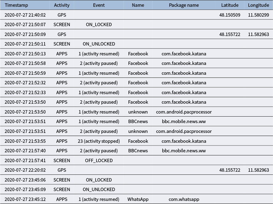
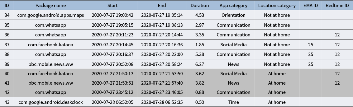
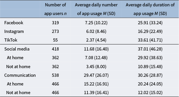


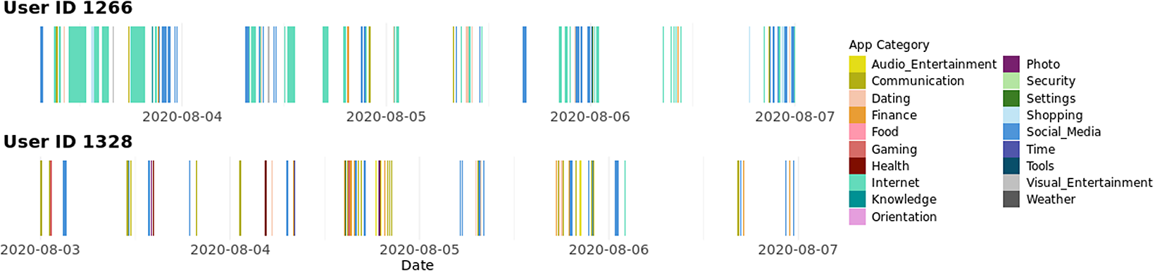

 Open access