


1. Introduction
The pandemic crisis brought lockdowns, elevated morbidity and death rates and increased public health costs worldwide. At their core, these constituted a supply-side shock that was unprecedented in scale and scope. It resulted in deep recessions in both advanced and developing regions, which left behind numerous impediments to future economic progress, including slower capital accumulation, human capital hysteresis and the impairment of “just in time” trade and supply chain linkages (Kose et al., Reference Kose, Nagle, Ohnsorge and Sugawara2020; World Bank, Reference Bank2020). Notwithstanding historically high levels of sovereign debt, very low policy interest rates appeared supportive of the substantial fiscal and monetary expansions that ensued in response.Footnote 1 This paper provides a theoretical and empirical analysis of the fiscal and monetary origins of the post-pandemic inflationary surge. We develop a theoretical framework in which both outside and inside money are treated as produced financial assets with portfolio and transaction demand. We empirically test this theory using panel data for 17 advanced economies from 1870 to 2016, as well as the years surrounding World War II (WWII). Empirically, we find that fiscal expansions that increase public debt are often accompanied by monetary expansions and inflation.
Conventional theory suggests that the combination of supply contractions and responsive fiscal and monetary expansions should not only raise sovereign debt overhangs but also bolster inflationary forces (Goodhart and Pradhan, Reference Goodhart and Pradhan2020; Ha et al., Reference Ha, Kose and Ohnsorge2021). Yet, while the pandemic raged, spokespeople for treasuries and central banks rarely offered future inflation as a stated concern.Footnote 2 While an established literature had suggested that at least some inflation was very likely in response to the fiscal expansions of the time (Omeokwe, Reference Omeokwe2020), especially given central bank purchases of newly issued government debt, there was clearly misdiagnosis (Koch & Noureldin, Reference Koch and Noureldin2024). This is explained by Reis (Reference Reis2022) as a welcoming by central banks of a return to modest inflation after decades of fighting deflationary forces. Reis asserts that inflation arose because central banks allowed it to, facing severe policy uncertainty and incorrectly assuming that inflation expectations were firmly anchored within target bands.Footnote 3
The hyperinflations in Europe in the 1930s, in Latin America in the 1970s and 80s and in the former Soviet Union in 1990 are prominent examples of monetised fiscal expansions in the face of negative shocks, economic interest in which goes back to Fisher (Reference Fisher1933). Such bursts of inflation do appear to have occurred with declining ferocity, in the advanced economies at least, following the commodity crises of the 1970s, the Asian financial crisis of the late 1990s (Azwar and Tyers, Reference Azwar and Tyers2020), and the global financial crisis of 2008 (Reinhart and Rogoff, Reference Reinhart and Rogoff2009). Nonetheless, temporary and substantial inflation accompanied the recovery from the crises of the 1970s and 1990s, both in advanced economies and in Asia and Latin America. While improved coordination between the central banks of the advanced economies during the “great moderation” period was a stabilising influence, as Reinhart & Rogoff indicate, the post-pandemic inflation surge should not have come as a surprise.
Moreover, to the extent that sovereign debt might have been the major concern, Kose et al. (Reference Kose, Nagle, Ohnsorge and Sugawara2020), in a survey, identified three “waves” of global debt that occurred following the demise of the Bretton Woods system and before the pandemic. Each wave ended in a financial crisis. Yet, in an influential pre-pandemic paper, Blanchard (Reference Blanchard2019) concluded that sovereign debt could be “grown out of” so long as the real growth rate were to exceed the real interest rate on long maturity debt.
In an earlier policy environment, responses to the pandemic might have included “financial repression” and price controls, which had characterised the recoveries from WWII in Europe and the US. Government bond yields were then regulated to sustain the demand for government debt, as were product price increases.Footnote 4 Indeed, as the subsequent reviews by Reinhart and Rogoff (Reference Reinhart and Rogoff2009, Reference Reinhart and Rogoff2010, Reference Reinhart and Rogoff2011, Reference Reinhart and Rogoff2013, Reference Reinhart and Rogoff2014) establish, recoveries from such crises in the past had moderated inflation via mixes of financial repression, public and private debt restructuring, capital controls and product price controls. Modern, open democracies are not well equipped for such interventions, making the eventual emergence of inflation seem inevitable.
Research on the policy responses emerged quickly after the pandemic had begun. Goodhart and Pradhan (Reference Goodhart and Pradhan2020) confirmed that the pandemic induced a negative supply shock, describing it as the dividing line between the deflationary forces of the previous three decades and the anticipated resurgence of inflation over the next two decades. McKibbin and Fernando (Reference McKibbin and Fernando2020) were among those who analysed the global economic consequences, focusing on the real output effects of the pandemic rather than the policy response. Since then, much of the related research has concerned the Phillips Curve and the associated responsiveness of inflation to labour market tightness.Footnote 5
Harding et al. (Reference Harding, Linde and Trabandt2023) build on these approaches, showing that imperfect competition creates a kink in the Phillips Curve, leading to a better fit with the data. Ball et al. (Reference Ball, Leigh and Mishra2022) and di Giovanni et al. (Reference di Giovanni, Kalemli-Özcan, Silva and Yıldırım2023), also focus on supply side shocks, but include energy-specific shocks and supply chain restrictions. Bernanke and Blanchard (Reference Bernanke and Blanchard2025) offer an analysis that rejects tight labour markets as the principal source of the inflation surge, identifying its origin as rises in “prices given wages”. Strong as this literature is in addressing the recessionary consequences of the pandemic, it tends to overlook the deflationary experience of prior decades and the sudden transition to inflation. Our paper sheds light on these omissions.Footnote 6
We begin by applying some elemental theory to the fundamental determinants of inflation. Drawing on Tobin’s (Reference Tobin1969) “general equilibrium” theory of monetary economics, our analysis treats both outside and inside money as central bank-monopoly-supplied financial assets facing portfolio and transaction demand.Footnote 7 Following Patinkin (Reference Patinkin1965), we allow portfolio demand to respond to relative expansions of wealth and explicitly account for the monetisation of fiscal deficits and the cost of sovereign debt. Unconventional monetary policy (UMP) is included, given the period’s proximity of short yields to zero lower bounds, along with demand repression, real wage changes, financial volatility and expectations over future inflation, output and capital returns. The analytical results indicate that inflation forces, while complex, were elevated by the pandemic’s supply contractions, and by the expansionary monetary and fiscal policies adopted in response.
We then focus on those determinants from this analysis that are historically observable, re-examining the relationships between supply and demand side shocks, debt, and inflation, using a panel vector autoregression (PVAR) of 17 advanced economies. In our long run analysis we consider the period from 1870 to 2016. As an event study, we also examine the years surrounding WWII. We find that, over a century, as well as more recently, episodes of fiscal expansions that raise public debt have typically been associated with accommodative monetary expansions and subsequent inflation. Indeed, following the pandemic, both private and sovereign debt reached historically high levels, and barring further negative shocks and associated pessimism, rising inflation would have been difficult to avoid during recovery.
Our analysis highlights that while fostering growth to control sovereign debt may have been appropriate during the two decades preceding the pandemic, it was a less viable response in the fraught economic environment that followed the pandemic. Indeed, the timing and immediate consequences of the Ukraine War and the subsequent turmoil in the Middle East presaged supply restrictions, particularly for energy and agricultural commodities. These extended the pandemic-initiated contractionary forces and forestalled the option for accelerated growth. In any case, the emergent policy responses emphasised monetary and fiscal stimulants that are not in themselves the foundations for long-run growth (Woo and Kumar Reference Woo and Kumar2015).
The rest of the paper is organised as follows. The following section uses a theoretical model to assess the short run consequences of the combined shocks that constituted the pandemic. Section 3 then describes our econometric investigation of the links between inflation and its contributing forces following negative historical shocks to selected advanced economies. Section 4 concludes.
2. Elemental theory
Here, we construct an elemental demand-side model that includes explicit treatment of portfolio money, UMP and the monetisation of fiscal expansions, along with other supply and demand-side determinants of inflation. By contrast with recent literature on the fiscal theory of inflation (Cochrane, Reference Cochrane2023), we explicitly track the quantity of money following Tobin’s (Reference Tobin1969) general equilibrium theory and the subsequent work of Sargent and Wallace (Reference Sargent and Wallace1981), among others. As in this literature, we also allow for monetary expansions as a means of addressing fiscal deficits through seignorage.Footnote 8
The importance of the quantity of money and its role in private portfolios is also consistent with the recent work of Brunemeier and Sannikov (Reference Brunnermeier and Sannikov2016), who treat money as a safe asset in a risky economy, sourced “inside” through liquid private debt instruments and “outside” by central banks.Footnote 9 In the context of this riskiness, we seek to identify links to immediate inflation outcomes, for which it is sufficient to consider single realisations of shocks to the many risky variables involved. Thus, while we include expectations over real output, the real rate of return on investment and the inflation rate, along with ambient volatility, our analytics are deterministic.
We consider a static, demand-side model of the global, closed macroeconomy with government. This economy supplies two things: goods and a commodity called “money” which comprises both conventional, outside, and “inside” variants. These forms of money are real assets by virtue of their tradability with goods at an exchange rate indicated by the price level and, as per Patinkin, Tobin and Brunnermeier et al., they are key elements of the wealth portfolio. The outside money component is the monetary base, which is supplied by a stylised central bank, and the inside money component is supplied by qualified financial institutions operating independently of government.Footnote 10
Conventionally, this money not only plays the role of “safe asset” in the wealth portfolio but its central purpose is to serve a “cash in advance” constraint on all transactions. Its quantity is supplied at zero fixed cost and negligible marginal cost and, thus, the period increment to its supply, ${\unicode{x0394}} M^{S}$
, is added to nominal factor income as seignorage accruing to the central bank and financial institutions.
${\unicode{x0394}} M^{S}$
, is added to nominal factor income as seignorage accruing to the central bank and financial institutions.
The real value of newly issued money, ${\unicode{x0394}} m^{S}$
, must therefore be added to the net output of goods and services to yield the economy’s real GDP,
${\unicode{x0394}} m^{S}$
, must therefore be added to the net output of goods and services to yield the economy’s real GDP, $RGDP=y+{\unicode{x0394}} m^{S}$
. If the exchange rate between that money and goods (the price level) is P, so that
$RGDP=y+{\unicode{x0394}} m^{S}$
. If the exchange rate between that money and goods (the price level) is P, so that ${\unicode{x0394}} M^{S}=P\,{\unicode{x0394}} m^{S}$
, and the volume of goods and services supplied is y, we have that
${\unicode{x0394}} M^{S}=P\,{\unicode{x0394}} m^{S}$
, and the volume of goods and services supplied is y, we have that $GDP=P y+{\unicode{x0394}} M^{S}$
.Footnote
11
We assume that the private sector manages an endogenously constructed portfolio comprising long-maturity private assets, money and government debt, while the real output of products and the government’s fiscal position are exogenous, with government deficits indicating the issuance of new long-maturity government bonds.
$GDP=P y+{\unicode{x0394}} M^{S}$
.Footnote
11
We assume that the private sector manages an endogenously constructed portfolio comprising long-maturity private assets, money and government debt, while the real output of products and the government’s fiscal position are exogenous, with government deficits indicating the issuance of new long-maturity government bonds.
Unconventional monetary policy dominates in that the central bank prints money in exchange for at least a portion of the period’s newly issued, long maturity government bonds. The model determines a list of endogenous demand side variables that include the price level, P, real investment expenditure on physical capital i, the collective household’s real private saving, s H , the increment to real money balances, Δm S , the corresponding increment to real portfolio money holdings Δm P , the increment to the government’s real indebtedness to the private household, Δd GP , the real yield on the collective portfolio, r P ,Footnote 12 and the nominal yield on government debt, R G .
All coefficients, a, in our linear formulations are defined positive. Endogenous variables with zero subscripts indicate carry-in values from the previous period. Unless otherwise indicated, upper case variables are nominal, measured in money, while lower case variables are real, measured in units of output.
2.1 Institutional balances
For the collective private household, H, at the current price level, P, nominal saving, Ps H , covers gross nominal investment, Pi, the holding of all newly supplied central bank issue, ΔM B , and the increment to the privately held portion of newly issued government debt, ΔD GP .
 \begin{align} P s^{H}=Pi+{\unicode{x0394}} M^{B}+{\unicode{x0394}} D^{GP}. \end{align} ${\unicode{x0394}} M^{B}$
is the period change in the monetary base. On the income side, H earns nominal, net factor income, Py, where y is the net volume of output of products. It also earns income from the creation of liquid assets, or money, by the private financial sector, which is the difference between the changes in money supply and the monetary base:
${\unicode{x0394}} M^{B}$
is the period change in the monetary base. On the income side, H earns nominal, net factor income, Py, where y is the net volume of output of products. It also earns income from the creation of liquid assets, or money, by the private financial sector, which is the difference between the changes in money supply and the monetary base: ${\unicode{x0394}} M^{S}-{\unicode{x0394}} M^{B}$
. Finally, it earns debt service from the government at long maturity nominal yield
${\unicode{x0394}} M^{S}-{\unicode{x0394}} M^{B}$
. Finally, it earns debt service from the government at long maturity nominal yield $R^{G}$
. So H’s total nominal income must balance with H’s expenditures on consumption, assets and tax:
$R^{G}$
. So H’s total nominal income must balance with H’s expenditures on consumption, assets and tax:
 \begin{align} P y+\left({\unicode{x0394}} M^{S}-{\unicode{x0394}} M^{B}\right)+R^{G}D_{0}^{GP}=P c+P s^{H}+T=P c+\left(P i+{\unicode{x0394}} M^{B}+{\unicode{x0394}} D^{GP}\right)+T \end{align}
To complete the corresponding balance from the perspective of the government we need its incomings, which include overall debt increases (the sale of bonds to both the private sector and the central bank), ΔD
G
= ΔD
GP
+ΔD
GCB
, and central bank profits. We assume the central bank’s activities, including its money printing, incur negligible fixed and marginal cost. Its accounting profits, $\sqcap ^{CB}$
, therefore include seigniorage and central bank portfolio earnings, which here include only government bond returns:
$\sqcap ^{CB}$
, therefore include seigniorage and central bank portfolio earnings, which here include only government bond returns: $\sqcap ^{CB}={\unicode{x0394}} M^{B}+R^{G}D_{0}^{GCB}$
.
$\sqcap ^{CB}={\unicode{x0394}} M^{B}+R^{G}D_{0}^{GCB}$
.
Government outgoings comprise spending on products, G, and debt service at nominal yield R G . Equating incomings with outgoings we have:
 \begin{align} {\unicode{x0394}} D^{G}+\left({\unicode{x0394}} M^{B}+R^{G}D_{0}^{GCB}\right)+T=G+R^{G}D_{0}^{G}. \end{align}
Note, first, that ΔD
G
−ΔD
GCB
= ΔD
GP
in (3). Assume that the central bank implements “unconventional monetary policy” or quantitative easing, and so it prints money to acquire (without necessarily monopolising) government debt ( ${\unicode{x0394}} D^{GCB}={\unicode{x0394}} M^{B}$
). These modifications allow us to substitute the adapted (3) for ΔD
GP
, in (2), with the result that:
${\unicode{x0394}} D^{GCB}={\unicode{x0394}} M^{B}$
). These modifications allow us to substitute the adapted (3) for ΔD
GP
, in (2), with the result that:
 \begin{equation*} P y+({\unicode{x0394}} M^{S}-{\unicode{x0394}} M^{B})+R^{G}D_{0}^{GP}=P c+P i+T+{\unicode{x0394}} M^{B}+(G-T)+R^{G}D_{0}^{GP}-{\unicode{x0394}} M^{B}-{\unicode{x0394}} M^{B}. \end{equation*}
Eliminating internal exchanges, this simplifies to the expenditure identity in nominal terms, which equates nominal income, from the supply of products and new money, to total expenditure:
 \begin{align} P y+{\unicode{x0394}} M^{S}=GDP=P c+P i+G .\end{align}
2.2 Financial equilibrium
From (1) and (2) the source and distribution of nominal private saving is:
 \begin{align} P s^{H}=P y+\left({\unicode{x0394}} M^{S}-{\unicode{x0394}} M^{B}\right)+R^{G}D_{0}^{GP}-T-P c=P i+{\unicode{x0394}} M^{B}+{\unicode{x0394}} D^{GP} .\end{align}
But real private consumption, c, and real investment, i, are both behavioural. Real private consumption is linked, in turn, to real private saving, which is what we formulate here. It depends on current, real private income, y, expected future real income, $y^{e}$
, the increment to the real wealth of the lower 90% of households by income,
$y^{e}$
, the increment to the real wealth of the lower 90% of households by income, ${\unicode{x0394}} w^{L}$
, and the real, long maturity rate of return on portfolio assets,
${\unicode{x0394}} w^{L}$
, and the real, long maturity rate of return on portfolio assets, $r^{P}$
Footnote
13
:
$r^{P}$
Footnote
13
:
 \begin{align} s^{H}=\left(a_{0}^{S}+\rho ^{S}\right)+a_{1}^{S}\,\left(y_{0}+{\unicode{x0394}} y\right)-a_{2}^{S}\,y^{e}-a_{3}^{S}{\unicode{x0394}} w^{L}+a_{4}^{S}\,r^{P}\, ,\end{align}
where ρ S is a shifter to represent the extent to which consumption is restricted by pandemic shutdowns and therefore real saving may be temporarily enlarged. The emphasis on the change in real wealth of the lower 90% of households reflects the fact that these households’ dominant asset is illiquid property. When the wealth embodied in this property rises it is well established that their consumption rises and their saving from disposable income declines. Very high-income households manage more liquid and diversified portfolios with smoothed consumption less affected by portfolio value changes (Luc et al., Reference Luc, Lamarche and Savignac2015). As we assume in the next section, a rise in their wealth, Δw H , affects their portfolio demand for money.Footnote 14
Real, net investment requires the issuance of private, long maturity, debt instruments. It depends positively on the expected real rate of return on capital net of depreciation, $r^{Ke}$
, and negatively on the real rate of return on long maturity assets in the collective portfolio, r
P
:
$r^{Ke}$
, and negatively on the real rate of return on long maturity assets in the collective portfolio, r
P
:
 \begin{align} i=a_{0}^{i}+a_{1}^{i}\,r^{Ke}-a_{2}^{i}\,r^{P}\,\hspace{0pt} \end{align}
From (4) nominal government saving is equal to its debt retirement, and private saving is from (5). Total nominal saving by source in the current period then emerges as nominal GDP (= Py + ΔM S ) less private consumption and government expenditure:
 \begin{align} P\left(s^{H}+s^{G}\right)& =\left[P y+\left({\unicode{x0394}} M^{S}-{\unicode{x0394}} M^{B}\right)+R^{G}D_{0}^{GP}-T-P c\right]+\left[-{\unicode{x0394}} D^{G}\right] \nonumber\\& =\left[P y+\left({\unicode{x0394}} M^{S}-{\unicode{x0394}} M^{B}\right)+R^{G}D_{0}^{GP}-T-P c\right]+\left[\left(T-G\right)+{\unicode{x0394}} M^{B}-R^{G}D_{0}^{GP}\right] \nonumber\\& =\left(P y+{\unicode{x0394}} M^{S}\right)-P c-G .\end{align}
The total saving on its LHS must be equal to the distribution of this saving—private acquisitions of physical capital (Pi), newly printed money (ΔM B ) and government debt, as well as government saving that takes the form of retiring its own debt:
 \begin{align} P\left(s^{H}+s^{G}\right)=\left(P y+{\unicode{x0394}} M^{S}\right)-P c-G=P i+{\unicode{x0394}} M^{B}-{\unicode{x0394}} D^{GCB}=Pi .\end{align}
Since the monetary expansion finances only the non-exclusive purchase by the central bank of newly issued government debt, we have, as in the previous section, ΔM
B
= ΔD
GCB
, and so (9) simplifies to the expenditure identity (4). From (2) we have that investment and consumption sum to disposable income, or the disposal identity for the private household: $P y+({\unicode{x0394}} M^{S}-{\unicode{x0394}} M^{B})+R^{G}D_{0}^{GP}=P c+P s^{H}+T$
. Using this to substitute for Pc in (9), we have:
$P y+({\unicode{x0394}} M^{S}-{\unicode{x0394}} M^{B})+R^{G}D_{0}^{GP}=P c+P s^{H}+T$
. Using this to substitute for Pc in (9), we have:
 \begin{equation*} P s^{H}-P i=G-T-{\unicode{x0394}} M^{B}+R^{G}D_{0}^{GP}=-P s^{G}={\unicode{x0394}} D^{G}. \end{equation*}
Then substituting the behavioural relationships for saving and investment on the LHS we have the financial market equilibrium condition:
 \begin{equation*} \begin{array}{l} P\left[\left(a_{0}^{S}+\rho ^{S}\right)+a_{1}^{S}\,\left(y_{0}+{\unicode{x0394}} y\right)-a_{2}^{S}\,y^{e}-a_{3}^{S}{\unicode{x0394}} w^{L}+a_{4}^{S}\,r^{P}\right]-P\left[a_{0}^{i}+a_{1}^{i}\,r^{Ke}-a_{2}^{i}\,r^{P}\,\right]\\ \quad =G-T-{\unicode{x0394}} M^{B}+R^{G}D_{0}^{GP} \end{array} \end{equation*}
from which we can solve for the real yield on the private portfolio. Before doing so, however, we need to link the nominal yield on government debt to the real private portfolio yield. These differ by the safe asset discount factor, γ<1, and expected inflation, so that
 \begin{align}R^G = \gamma r^P + \pi^e.\end{align}
With this substituted in the final term we can divide through by the price level and express real variables in lower case. We can then place the two sources of saving on the LHS and investment on the RHS, expressing financial market equilibrium condition $s^{H}+s^{G}=i$
in terms of exogenous variables:
$s^{H}+s^{G}=i$
in terms of exogenous variables:
 \begin{align} & \left[\left(a_{0}^{S}+\rho ^{S}\right)+a_{1}^{S}\,\left(y_{0}+{\unicode{x0394}} y\right)-a_{2}^{S}\,y^{e}-a_{3}^{S}{\unicode{x0394}} w^{L}+a_{4}^{S}\,r^{P}\right]+\left[t-g+{\unicode{x0394}} m^{B}-d_{0}^{GP}\gamma r^{P}-d_{0}^{GP}\pi ^{e}\right] \nonumber\\& \quad =\left[a_{0}^{i}+a_{1}^{i}\,r^{Ke}-a_{2}^{i}\,r^{P}\,\right] \end{align}
An algebraic solution for the real portfolio yield, r P , is readily obtained in terms of all the exogenous variables and the change in the real value of the monetary base, Δm B . We offer this in an Appendix. Before interpreting this relationship, however, we note our intention that the change in the real monetary base should be endogenous, and so we require behaviour for it.
2.3 The market for money
The period increment to the real money supply, Δm S , must equal the increment to the demand to hold real money balances, Δm D , which meet both portfolio and transactions demand:
 \begin{align} {\unicode{x0394}} m^{D}={\unicode{x0394}} m^{P}+{\unicode{x0394}} m^{T}={\unicode{x0394}} m^{S} .\end{align}
Here real transaction demand, m
T
, is proportional to nominal output, ${\unicode{x0394}} m^{T}\approx \phi {\unicode{x0394}} y$
, so the nominal equivalent is
${\unicode{x0394}} m^{T}\approx \phi {\unicode{x0394}} y$
, so the nominal equivalent is ${\unicode{x0394}} M^{T}=\phi (Py-P_{0}y_{0})$
. We then require behaviour for the increment to portfolio money demand, Δm
P
. For this, we posit that the share of money in portfolios depends positively on the level of general volatility, v. This dependence arises from the well-known tendency for portfolios to rebalance toward safe assets, usually cash and short maturity government bonds, the more risky higher-returning, private assets become. Portfolio money holdings also depend on the change in the size of the high-income wealth portfolio, Δw
H
, measured as its purchasing power over goods, and the real yield spread between money and productive assets:
${\unicode{x0394}} M^{T}=\phi (Py-P_{0}y_{0})$
. We then require behaviour for the increment to portfolio money demand, Δm
P
. For this, we posit that the share of money in portfolios depends positively on the level of general volatility, v. This dependence arises from the well-known tendency for portfolios to rebalance toward safe assets, usually cash and short maturity government bonds, the more risky higher-returning, private assets become. Portfolio money holdings also depend on the change in the size of the high-income wealth portfolio, Δw
H
, measured as its purchasing power over goods, and the real yield spread between money and productive assets: $r^{Me}-r^{P}$
, where the expected real yield on money is
$r^{Me}-r^{P}$
, where the expected real yield on money is $r^{Me}=P/P^{e}-1=-\pi ^{e}$
.
$r^{Me}=P/P^{e}-1=-\pi ^{e}$
.
The dependence on real wealth is here intended to capture the difference in recent decades between the growth rates of real output and the purchasing power of the high-income real wealth portfolio at consumer product prices. A shock to real high-income wealth, w H , in the absence of a corresponding shock to real output and low-income wealth, w L , is therefore suggestive of a shift to greater inequality. It is our assumption that, where the wealth shock advantages high-income earners, it suggests a larger sized wealth portfolio and hence increased need for portfolio money to balance the liquid share (Agarwal et al., Reference Agarwal, Chua, Ghosh and Song2020; Lenza and Slacalek, Reference Lenza and Slacalek2019; Wei et al., Reference Wei, Wu and Zhang2019; Jawadi et al., Reference Jawadi, Sousa and Traverso2017).
To represent these behaviours in the portfolio money equation we adopt terms in general volatility, high-income real wealth and the spread between the real rates of return on money and returning assets:
 \begin{align} {\unicode{x0394}} m^{P}& =a_{0}^{P}+a_{1}^{P}v+a_{2}^{P}{\unicode{x0394}} w^{H}+a_{3}^{P}\left(r^{Me}-r^{P}\right)=a_{0}^{P}+a_{1}^{P}v+a_{2}^{P}{\unicode{x0394}} w^{H}-a_{3}^{P}\left(r^{P}+\pi ^{e}\right) \nonumber\\& =a_{0}^{P}+a_{1}^{P}v+a_{2}^{P}{\unicode{x0394}} w^{H}-a_{3}^{P}R^{P} ,\end{align}
where R P is the nominal yield on long maturity assets. Thus, we have the conventional dependence of the demand for real money balances on the nominal yield.Footnote 15 We can therefore write the change in the real money supply that meets demand as:
 \begin{align} {\unicode{x0394}} m^{D}={\unicode{x0394}} m^{S}=a_{0}^{P}+a_{1}^{P}v+a_{2}^{P}{\unicode{x0394}} w^{H}-a_{3}^{P}\left(r^{P}+\pi ^{e}\right)+\phi {\unicode{x0394}} y \end{align}
To complete the determination of the real equilibrium yield, r
P
, we require an expression for the change in the real monetary base, Δm
B
, to substitute into (11). This is the real value of period central bank purchases $(M^{B}/P-M_{0}^{B}/P_{0})\approx {\unicode{x0394}} M^{B}/P={\unicode{x0394}} m^{B}$
, where M
B
and m
B
are the nominal and real measures. The corresponding totals of safe, liquid assets available are the money supplies, M
S
and m
S
, which are traditionally larger than the monetary base by a factor equal to the money multiplier. This factor depends negatively on private cash holdings relative to deposits, and commercial bank liquidity reserves, both of which tend to rise when there is an increase in general financial market volatility, v. Here we achieve this effect linearly:
$(M^{B}/P-M_{0}^{B}/P_{0})\approx {\unicode{x0394}} M^{B}/P={\unicode{x0394}} m^{B}$
, where M
B
and m
B
are the nominal and real measures. The corresponding totals of safe, liquid assets available are the money supplies, M
S
and m
S
, which are traditionally larger than the monetary base by a factor equal to the money multiplier. This factor depends negatively on private cash holdings relative to deposits, and commercial bank liquidity reserves, both of which tend to rise when there is an increase in general financial market volatility, v. Here we achieve this effect linearly:
 \begin{align} {\unicode{x0394}} m^{S}-{\unicode{x0394}} m^{B}=a_{0}^{M}-a_{1}^{M}\nu,\ \text{so that}\ {\unicode{x0394}} m^{B}={\unicode{x0394}} m^{S}-a_{0}^{M}+a_{1}^{M}\nu .\end{align}
Expanding for Δm S from (14) then yields:
 \begin{align} {\unicode{x0394}} m^{B} & ={\unicode{x0394}} m^{P}+{\unicode{x0394}} m^{T}-a_{0}^{M}+a^{M}v=a_{0}^{P}+a_{1}^{P}v+a_{2}^{P}{\unicode{x0394}} w^{H}-a_{3}^{P}\left(r^{P}+\pi ^{e}\right)+\phi {\unicode{x0394}} y-a_{0}^{M}+a_{1}^{M}v \nonumber\\& =\left(a_{0}^{P}-a_{0}^{M}\right)+\left(a_{1}^{P}+a_{1}^{M}\right)v+a_{2}^{P}{\unicode{x0394}} w^{H}-a_{3}^{P}\left(r^{P}+\pi ^{e}\right)+\phi {\unicode{x0394}} y .\end{align}
Substituting this for Δm B in (11), yields the equilibrium real private portfolio rate of return, as detailed in the Appendix. The signs of the coefficients indicate that this relationship has the following structure:Footnote 16
 \begin{align} \begin{array}{rcccccccc} - & - & + & + & -& -& +& +& +\\ r^{P}=r^{P} [{\unicode{x0394}} y, & \rho ^{S}, & \left(g-t\right), &{\unicode{x0394}} w^{L}, & {\unicode{x0394}} w^{H},&v,& \pi ^{e}, & y^{e}, & r^{Ke} ] \end{array} .\end{align}
Bearing in mind that we seek the effects on the endogenous real yield of changing one exogenous variable while keeping all the others constant, we can readily explain the signs of these coefficients. The first, the real output shock, is negative because more real income shifts saving to the right and reduces the equilibrium yield. The second, a boost to saving because of consumption restrictions or taste changes, is negative because it shifts saving supply so as also to reduce the equilibrium yield. The third, the fiscal response indicated by the size of the fiscal deficit, is positive because of the usual crowding out effect of increased government expenditure raises $r^{P}$
. The fourth indicates that a positive shock to the real wealth of the lower 90% of households raises consumption, reduces saving and therefore raises the real yield. The fifth concerns the real wealth of the top 10% of households. Their restoration of liquidity balance requires a rise in portfolio money, which constrains investment in returning assets and therefore reduces the issue of assets, raises their prices and reduces their yields.
$r^{P}$
. The fourth indicates that a positive shock to the real wealth of the lower 90% of households raises consumption, reduces saving and therefore raises the real yield. The fifth concerns the real wealth of the top 10% of households. Their restoration of liquidity balance requires a rise in portfolio money, which constrains investment in returning assets and therefore reduces the issue of assets, raises their prices and reduces their yields.
The sixth, which is general financial volatility, affects the real yield negatively, by two mechanisms. First, since it induces a retreat from investment in returning assets that reduces bond or equity issues, it raises asset prices and reduces the real yield. Second, by inducing cash holding, increased volatility raises the real monetary base relative to the chosen level of overall real money balances, which implies greater cash accumulation by commercial banks and households and hence less investment, reducing the real yield. The seventh, the expected rate of inflation, affects the real yield positively, again via two mechanisms. First, greater expected inflation raises the government’s nominal debt service burden and so reduces its own saving or raises the fiscal deficit. Second, greater expected inflation raises the opportunity cost of holding portfolio money, raising investment in physical capital and hence the demand for loanable funds. The eighth, the level of expected future real income, $y^{e}$
, is positive because a consumption-smoothing household reduces saving if expected future income rises. And the ninth, the effect of an increment to the expected real net yield on physical capital is to raise investment in such capital, which therefore raises the market real yield.
$y^{e}$
, is positive because a consumption-smoothing household reduces saving if expected future income rises. And the ninth, the effect of an increment to the expected real net yield on physical capital is to raise investment in such capital, which therefore raises the market real yield.
Global financial and money markets with a UMP money Shock.
Note: An unconventional (UMP) monetary expansion is represented. The saving, investment and money demand expressions are from (11) and (14) in the text, which have the following behaviour:
 \begin{align*} \begin{array}{rcccc} +&+&-&-&+ \\ s^{D}=s^{H}(\rho ^{S},& {\unicode{x0394}} y,&y^{e},&{\unicode{x0394}} w^{L},&r^{P}) \end{array} \begin{array}{rcccc} +&-&+&-&- \\ +s^{G}(t,&g,&{\unicode{x0394}} m^{B},&\pi ^{e},&r^{P}) \end{array}\begin{array}{rcccccccc} +&+&-&-&+&-&+&-&+\\ =s^{D}(\rho ^{S},& {\unicode{x0394}} y,&y^{e},&{\unicode{x0394}} w^{L},&t,&g,&{\unicode{x0394}} m^{B},&\pi ^{e},&r^{P}) , \end{array}\begin{array}{rc} +&-\\ i=i(r^{Ke},&r^{P}) , \end{array} \end{align*}
 \begin{align*} \begin{array}{rcccc} +&+&+&-&-\\ m^{D}=m_{0}^{D}+{\unicode{x0394}} m^{D}({\unicode{x0394}} y,&{\unicode{x0394}} w^{H},&v,&\pi ^{e},&r^{P}). \end{array} \end{align*}
The rightward shift in the saving curve is here due to the central bank’s acquisitions, which reduce the long maturity yield and raise real money balances, $m^{S}\uparrow$
. These acquisitions are financed by a nominal monetary expansion,
$m^{S}\uparrow$
. These acquisitions are financed by a nominal monetary expansion, $M^{B}\uparrow$
. From this shock alone, inflation only results if
$M^{B}\uparrow$
. From this shock alone, inflation only results if $\hat{P}=\hat{M}^{B}+\hat{\mu }-\hat{m}^{S}\gt 0$
, where μ is the money multiplier—that is, if the nominal expansion exceeds that in real money balances.
$\hat{P}=\hat{M}^{B}+\hat{\mu }-\hat{m}^{S}\gt 0$
, where μ is the money multiplier—that is, if the nominal expansion exceeds that in real money balances.

2.4 An almost conventional graphical representation
The financial equilibrium condition (11) suggests a conventional, graphical depiction of the financial market, or the market for loanable funds. The money market equilibrium condition (14) also suggests a graphical representation. Both are included in Figure 1, which depicts two interdependent asset markets: the global market for long-maturity assets and the corresponding global market for liquid assets that we call money. The vertical axis in both diagrams represents the real yield on the private, collective portfolio of primarily long maturity assets, $r^{P}$
, while the horizontal axes represent the levels of real saving, real investment and real money balances. In the market for money, we represent expected inflation as one of a number of shifters of the money demand curve, so that the two vertical axes are common.
$r^{P}$
, while the horizontal axes represent the levels of real saving, real investment and real money balances. In the market for money, we represent expected inflation as one of a number of shifters of the money demand curve, so that the two vertical axes are common.
In considering the effects of shocks graphically, it is best to begin with displacements of the two financial market curves, as indicated by the shifters noted below the diagram. These result in a changed real yield on the collective asset portfolio, $r^{P}$
, which then represents the opportunity cost of holding money in that portfolio. Real money balances then emerge from the level of this yield and the real money demand function. The figure illustrates a UMP expansion from which a resulting inflation is likely but not guaranteed. The ambiguity stems from the central bank’s acquisition of long maturity assets raising their price and suppressing their yield, causing a rise in the demand for real money balances. For an inflation to eventuate the associated nominal monetary expansion that finances the bond purchases must be proportionally larger.
$r^{P}$
, which then represents the opportunity cost of holding money in that portfolio. Real money balances then emerge from the level of this yield and the real money demand function. The figure illustrates a UMP expansion from which a resulting inflation is likely but not guaranteed. The ambiguity stems from the central bank’s acquisition of long maturity assets raising their price and suppressing their yield, causing a rise in the demand for real money balances. For an inflation to eventuate the associated nominal monetary expansion that finances the bond purchases must be proportionally larger.
Of course, we can imagine many other shocks to the shifting variables indicated at the foot of the diagram. One of these shocks is to inflation expectations. If agents expect deflation it further weighs against the monetary expansion, making deflation more likely in spite of it. To quantify this represented behaviour, and to see its effect on actual inflation, we require a corresponding formulation for real money balances.
2.5 The increment to the real monetary base
The period addition to the level of the real monetary base, given the exogenous conditions, is readily constructed by substituting (17) for $r^{P}$
into (16). We offer the complete solution in the Appendix. Its determinants can be signed as:
$r^{P}$
into (16). We offer the complete solution in the Appendix. Its determinants can be signed as:
 \begin{align} \begin{array}{rcccccccc} +& +& -& -& +& +& -& -& -\\ {\unicode{x0394}} m^{B}= [{\unicode{x0394}} y, & \rho ^{S}, & \left(g-t\right), & {\unicode{x0394}} w^{L}, &{\unicode{x0394}} w^{H}, & v,& \pi ^{e},&y^{e},&r^{Ke}] \end{array} .\end{align}
Most significantly, relative to the corresponding expression for real, full money balances, this expression has a stronger positive response to general volatility.
Again, we can explain the emerging signs of the coefficients.Footnote 17 That of Δy is positive, since a rise in output also raises saving and reduces the real yield, which accommodates higher real money balances. A rise in the level of real transactions demand for money relative to real income bolsters this effect. That of consumption restriction, and therefore a rise in the saving shifter, ρ S , is also positive, since this also reduces the real yield and hence the opportunity cost of holding money. That of the fiscal deficit is negative. If the government deficit increases, the real yield rises, raising the opportunity cost of holding money and so implying decreased real money balances. A positive shock to the real wealth of the lower 90% of households raises consumption, reduces saving and therefore raises the real yield, raising the opportunity cost of holding money and reducing real money balances. A corresponding shock to the real wealth of the top 10% of households requires the restoration of their portfolio’s liquidity balance and therefore a rise in portfolio money. This constrains investment in returning assets and therefore reduces the issue of new debt or equity, raising their prices and reducing their yields.Footnote 18
That of general volatility, v, is positive. This reflects both the effect of volatility in discouraging investment and so reducing real yields and its direct effect on portfolio management that takes for form of a retreat to money holding. In the case of the period change to the real monetary base, it also reflects the tendency for worker households to hold more cash and commercial banks to hold greater liquidity reserves. That of $\pi ^{e}$
is negative. Beyond the effect on the real yield discussed previously, a positive shock to expected inflation increases the opportunity cost of holding money, causing a leftward shift in Figure 1’s real money demand curve. That of
$\pi ^{e}$
is negative. Beyond the effect on the real yield discussed previously, a positive shock to expected inflation increases the opportunity cost of holding money, causing a leftward shift in Figure 1’s real money demand curve. That of $y^{e}$
is negative, since if higher future income is expected, current saving decreases and the real yield rises, implying reduced real money balances. Finally, that of
$y^{e}$
is negative, since if higher future income is expected, current saving decreases and the real yield rises, implying reduced real money balances. Finally, that of $r^{Ke}$
is negative, since investment optimism raises real investment demand. If current output stays constant, there is a higher real yield and this requires reduced real money balances. We can now assess the implications of these analytical results for future inflation rates.
$r^{Ke}$
is negative, since investment optimism raises real investment demand. If current output stays constant, there is a higher real yield and this requires reduced real money balances. We can now assess the implications of these analytical results for future inflation rates.
2.6 The determinants of inflation
From (17) and (18) we have the signed determinants of the real long rate and the period change in the real monetary base. These pin down the real variables that represent the purchasing power of the monetary base over products. However, the actual rate of inflation, π, depends on the path of the nominal money supply, M
S
, and from a policy standpoint, on the path of the nominal monetary base, M
B
. By definition, $M^{S}=P m^{S}$
, but also
$M^{S}=P m^{S}$
, but also $M^{B}=P m^{B}$
, so that
$M^{B}=P m^{B}$
, so that $\pi =\hat{P}=\hat{M}^{B}-\hat{m}^{B}$
. Central banks can only affect
$\pi =\hat{P}=\hat{M}^{B}-\hat{m}^{B}$
. Central banks can only affect $\hat{M}^{B}$
, and the period increment to the real monetary base is endogenous, from (18). Thus inflation depends on the rate of exogenous monetary expansion,
$\hat{M}^{B}$
, and the period increment to the real monetary base is endogenous, from (18). Thus inflation depends on the rate of exogenous monetary expansion, $\hat{M}^{B}$
, and the endogenous change in the real monetary base:
$\hat{M}^{B}$
, and the endogenous change in the real monetary base:
 \begin{align*} \pi \cong \frac{{\unicode{x0394}} P}{P_{0}}=\frac{{\unicode{x0394}} M^{B}}{M_{0}^{B}}-\frac{{\unicode{x0394}} m^{B}}{m_{0}^{B}}\cong \hat{M}^{B}-\hat{m}^{B}\left({\unicode{x0394}} y,\rho ^{S},\left(g-t\right),{\unicode{x0394}} w^{L},{\unicode{x0394}} w^{H},\,v,\, \pi ^{e},y^{e},r^{Ke}\right) .\end{align*}
This allows the consolidation and signing of determinants as:
 \begin{align} \begin{array}{rcccccccc} +\quad +\quad -& -& +& -& -& +& +& +\\ \pi =\hat{P}[\hat{M}^{B},\left(g-t\right),&{\unicode{x0394}} y,&\rho ^{S},&{\unicode{x0394}} w^{L},&{\unicode{x0394}} w^{H},&v,&\pi ^{e},&y^{e},&r^{Ke} ]\, \end{array} ,\end{align}
making clear that fiscal and monetary expansions are unambiguously inflationary as is a supply side contraction. Offsetting deflationary forces include a low-skill real wage decline, associated, for example, with technical change disadvantaging the low-skilled, and a similarly sourced high-skill wage increase. But then, the relaxation of demand restrictions, and declining output volatility would add to inflation, as would a return to optimism about future inflation, output and rates of return.Footnote 19
Apart from output recovery and the trend toward declines in real, low-skill wages, most of these deflationary drivers have not been observed for periods long enough for empirical testing. The global trend toward slower productivity and the widening of the real wage gap between the skilled and the low-skilled, has surely been a factor in the tendency to deflation in the years prior to the pandemic.Footnote 20 Our focus here, however, is on the investigation of the relative strengths of the dependencies on monetised fiscal expansions and short run output changes, which are addressed in Section 3.
2.7 Implications of the shutdown and macro policy shocks for real yields and inflation
Consider the implications of combined fiscal and monetary expansions experienced worldwide during the COVID-19 epidemic. Unfortunately, ambiguity is pervasive. Even the primary shutdown shocks are ambiguous for inflation. The health policy response to the pandemic restricts both output and consumption, so the inflationary effects of output restrictions are offset, at least to some extent, by associated consumption restrictions:
 \begin{equation*} \begin{array}{c} \,\qquad- \qquad-\\ \pi =\hat{P}[{\unicode{x0394}} y\downarrow ,\rho ^{S}\uparrow ] \end{array} .\end{equation*}
The effects of the pandemic on wealth and its distribution tend to suggest, at least thus far, that general housing wealth has declined while high-income portfolio wealth has increased, as suggested by persistently high equity prices. These are both deflationary forces, the first because less housing wealth causes less consumption and the second because increased portfolio wealth raises the demand for money holding and hence real money balances. By further opposing the inflationary effects of the supply shock, these additions therefore do nothing to address the ambiguity. Indeed, the outcome is made even murkier by the addition of a likely increase in general financial volatility, due possibly to the weakened accuracy of forecasts during the pandemic. This acts to cause a private retreat to money holding and conservative prudential behaviour by commercial banks, all of which is also deflationary:
 \begin{equation*} \begin{array}{ccccc}\qquad -&\!\!\!\! -&\!\!\!\! +&\!\!\!\! -&\!\!\!\! -\\ \pi =\hat{P}[{\unicode{x0394}} y\downarrow ,&\rho ^{S}\uparrow , &{\unicode{x0394}} w^{L}\downarrow ,&{\unicode{x0394}} w^{H}\uparrow ,&v\uparrow ] \end{array} .\end{equation*}
When we add the macro policy changes, which include historically large fiscal and monetary expansions, since these both contribute to inflation, it is more likely that the net outcome includes some inflation, though ambiguity persists:
 \begin{equation*} \begin{array}{ccccccc} \qquad+& \!\!\!\! +&\!\!\!\! -&\!\!\!\! +&\!\!\!\! -&\!\!\!\! -&\!\!\!\! -\\ \pi =\hat{P}[\hat{M}^{B}\uparrow ,&(g-t)\uparrow ,&{\unicode{x0394}} y\downarrow ,&{\unicode{x0394}} w^{L}\downarrow ,&{\unicode{x0394}} w^{H}\uparrow ,&\rho ^{S}\uparrow ,&v\uparrow ] \end{array} .\end{equation*}
Yet, key determining factors are whether expectations over inflation, future output and future returns are optimistic or pessimistic. If they remain pessimistic, they could cause deflation pressure that could, at least in theory, be large enough to offset the monetary and fiscal expansions:
 \begin{equation*} \begin{array}{ccc} \qquad +&\!\!\!\! +& \!\!\!\! + \\ \pi \downarrow =\hat{P}[\pi ^{e}\downarrow ,&y^{e}\downarrow ,&r^{Ke}\downarrow ] \end{array} .\end{equation*}
Thus, inflation depends not only on the rate of expansion of the nominal monetary base, but also on the extent to which the primary shocks and their consequences for the wealth distribution and volatility, and the macro policy responses, have a net tendency to reduce real money balances. This leaves the scale of any inflationary response to pandemic shocks indeterminate, at least without numerical analysis.Footnote 21,22
3. The empirics of historical monetary and fiscal effects
While all the determinants of inflation identified in our theory have not been observed over sufficient time to make them readily amenable to empirical testing, there are good long term records of monetary, fiscal and output changes for the advanced economies. We use data from the “Jordà-Schularick-Taylor Macrohistory Database” (release R.4), which contains macroeconomic data for 17 advanced economies over the period 1870–2016 (Jordà et al., Reference Jordà, Schularick, Taylor, Jordà, Schularick and Taylor2016). It shows clearly the inflations of the post WWI, post WWII, and 1970s energy/commodity crisis periods and it makes it possible to observe the relationship between macro performance in these episodes and prior fiscal and monetary policy.Footnote 23
In particular, we use these data to assess the relative strengths of the key fiscal and monetary determinants of inflation in the long run, with some emphasis on extraordinary events that parallel the pandemic. For this we turn to an empirical analysis of long-term associations over a century and a half, and an event study of the World War II period. In doing so, we highlight the particular dependence of inflationary episodes on fiscal expansions that increase sovereign debt and their accommodation by corresponding monetary expansions.
The objective of this empirical exercise is to document the historical relationship between public debt, money growth, and inflation. Other determinants of inflation are undoubtedly present across the sample of countries, and a comprehensive quantification and decomposition of these factors is an important direction for future research. Such an analysis could, for instance, employ a Markov-switching model as in Chen and Semmler (Reference Chen and Semmler2025). While we view this as a valuable avenue, we leave it for future work.
3.1 The econometric model
We estimate a structural panel vector auto-regression model using data from the Jordà-Schularick-Taylor Macrohistory Database, which suits our purpose because it covers a long time horizon that includes substantial shocks and associated fiscal policy changes. Indeed, during WWII many advanced economies experienced increases in sovereign debt that were of a similar magnitude to those during the recent pandemic.
The data over the entire period, since 1870, are illustrated in Figure 2. There are three particularly striking cases: Japan, Australia and the United States. For Japan, the public debt to GDP ratio exceeded two at the height of WWII and this coincided with a significant increase in broad money growth. By contrast, in the latter part of the sample, the mid-2000s saw Japan’s debt to GDP ratio approach 2.5, without any corresponding monetary expansion.Footnote 24 By 2020, however, Japan’s broad money was expanding rapidly. In that year it grew 7.3%: approximately five percentage points higher than the rise in the previous year.Footnote 25 A similar pattern is seen for the United States, where both the debt-to-GDP ratio and the growth rate of the broad money supply spiked during WWII. In 2020, the US money supply grew by 17.2%, an unprecedented rate since the 1940s. For Australia, debt levels rose both before and during WWII, whereas the broad money stock grew significantly during, but not immediately after, the war. Together, these patterns highlight the particular relevance of the 1940s as a reference period for our assessment of the post-pandemic recovery. Our empirical exercise uses the inflationary outcomes of the WWII period to infer likely changes associated with the recent pandemic, given similarities in the macroeconomic environments of many advanced economies in the two periods.
Pattern of real GDP growth, public debt to GDP ratio, broad money ratio and inflation in Australia, Japan and the US, (1870–2016).
Source: Constructed based on data from “Jordà-Schularick-Taylor Macrohistory Database”. The shaded bars indicate periods with output shocks: 1914–1918 (World War I), 1937–1950 (World War II), and 1973–1973 (1973 Oil Crisis).

The empirical model we employ is designed to test the relative strengths of the key determinants of inflation considered in the previous section, as summarised in equation (19). Given data limitations, we estimate a reduced system containing six variables from the microhistory database: real GDP, government revenue, public debt, private debt, broad money, and consumer price inflation. The use of a structural vector autoregression (SVAR) allows for the endogenous treatment of the inflation rate and an assessment of the role played by the key inflation drivers identified in (19). It also allows for the quantification of dynamic effects of shocks in system variables.Footnote 26
In what follows, i indexes the countries in the sample and t indexes time (all data is at the annual frequency). The countries included in the database are Australia, Belgium, Canada, Denmark, Finland, France, Germany, Italy, Japan, Netherlands, Norway, Portugal, Spain, Sweden, Switzerland, UK, and USA. We first generate impulse response functions for the entire sample period (1870–2016) and then focus our attention on the WWII period. While the patterns we uncover are present for both sample periods, the magnitude of the effects are typically larger for the WWII period. Formally, the reduced-form model we estimate is
 \begin{align} y_{it}=a_{0}+A_{1}y_{i,t-1}+A_{2}y_{i,t-2}+\gamma _{i}+u_{i,t} ,\end{align}
where the matrices $A_{1}$
and
$A_{1}$
and $A_{2}$
comprise the estimated parameters of the system,
$A_{2}$
comprise the estimated parameters of the system, $a_{0}$
is a vector of constants,
$a_{0}$
is a vector of constants, $\gamma _{i}$
is a vector of country fixed effects and
$\gamma _{i}$
is a vector of country fixed effects and $u_{i,t}$
is a vector of reduced-form errors (which are linear combinations of the structural errors). The dependent variable,
$u_{i,t}$
is a vector of reduced-form errors (which are linear combinations of the structural errors). The dependent variable, $y_{i,t}$
, is a vector of endogenous variables for country i at time t. Specifically,
$y_{i,t}$
, is a vector of endogenous variables for country i at time t. Specifically,
 \begin{align} y_{i,t}=\left[g_{i,t}^{Y},g_{i,t}^{G},d_{i,t}^{G},d_{i,t}^{P},g_{i,t}^{M},\pi _{i,t}\right] ,\end{align}
where $g_{i,t}^{Y}$
is the real GDP growth rate,
$g_{i,t}^{Y}$
is the real GDP growth rate, $g_{i,t}^{G}$
is the government revenue growth rate,
$g_{i,t}^{G}$
is the government revenue growth rate, $d_{i,t}^{G}$
is the growth rate of government debt,
$d_{i,t}^{G}$
is the growth rate of government debt, $d_{i,t}^{P}$
is the growth rate of private debt,
$d_{i,t}^{P}$
is the growth rate of private debt, $g_{i,t}^{M}$
is the growth rate of broad money and
$g_{i,t}^{M}$
is the growth rate of broad money and $\pi _{i,t}$
is the CPI inflation rate. All variables in
$\pi _{i,t}$
is the CPI inflation rate. All variables in $y_{i,t}$
are computed as year-on-year growth rates.
$y_{i,t}$
are computed as year-on-year growth rates.
We assess the stationarity of the variables in the system via unit root tests, including the Augmented Dickey-Fuller Test, Im-Pesaran-Shin Test, Levin-Lin-Chu Test, and Phillips–Perron Test. For each variable, the null hypothesis of non-stationarity is rejected at the 1% significance level, suggesting that all variables in the SVAR model are stationary.Footnote 27
We estimate this model on the balanced panel of 17 countries for the two aforementioned sample periods. Our final dataset contains growth rates of the macroeconomic variables in equation (21) across the 17 countries spanning the years 1870–2016. These countries have always been amongst the world’s most advanced, and so have had similar institutional structures and macro behaviour. The advantage of estimating a multi-country SVAR is therefore that it provides a significantly larger sample size compared to estimating the model using data from a single country, thereby increasing the precision of our estimates.Footnote 28 The model’s lag order is selected using the Schwarz Information Selection Criterion (SIC), which yields a specification with two lags.
To identify the parameters of the SVAR, we impose a series of exclusion restrictions on the variables in the system. We rely on the theory in Section 2 to synthesise these identification restrictions.Footnote 29 Specifically, following shocks to real GDP growth, government revenue growth adjusts simultaneously due to associated changes in tax revenue that occur on stable tax bases. Additionally, public debt and broad money growth also change simultaneously, reflecting the monetary financing of fiscal deficits. Inflation rates, public debt growth rates, and private debt growth rates also respond to changes in all other variables with a one-year lag. Under this set of identification assumptions, we estimate the Orthogonalized Impulse Response functions (OIRs) that identify the dynamic effects of shocks to one variable on the other variables in the system.Footnote 30
3.2 The long term results
The interdependencies amongst real GDP growth rates, the public debt growth rates (which are proxies for fiscal expansions), broad money growth rates and inflation rates in Australia, Japan, and the US, have been noted previously from Figure 2. The positive correlation between public debt growth and broad money growth is further seen in Figure 3 where, for each country, the two variables are plotted against each other and a linear regression line is estimated on each country’s data. The linear regressions all show positive slopes, thus indicating the positive correlation between public debt growth and broad money growth.
Nominal public debt growth vs. nominal broad money growth.
Source: Constructed based on data from “Jordà-Schularick-Taylor Macrohistory Database”.

Moving to the formal estimation results, we first present the OIRs for the entire period of 1870–2016 (T = 147) in Figure 4. These show that, when real GDP contracts, government revenues decline, and both public and private debt levels rise. Broad money and inflation both rise when public debt rises, and so inflation rates increase when broad money growth accelerates. When real GDP growth rates fall, there are declines in both broad money growth rates and inflation rates, likely because of long run changes in the transactions demand for money. Superficially, this contrasts with our very short run theoretical analysis in the previous section, where greater product supply relative to the money stock tends to reduce the price level. But it occurs because money growth declines as well, and our theoretical result in (19) is ambiguous when both output and money grow simultaneously. The bottom line, however, is that in the long run inflation has tended to move in the same direction as real GDP growth.Footnote 31
Orthogonalized impulse response functions for the full sample period (1870–2016), with 95% confidence intervals.
Note: Each panel shows the orthogonalized impulse response (OIR) function over a ten-year period following a one standard deviation (positive) structural innovation to variables in the SVAR. The blue lines show the impulse response, while the shaded bands represent 95% confidence intervals.
Source: Authors’ estimation of the SVAR model using 1870–2016 data.

3.3 The WWII period
The long run patterns are found to prevail (and are exacerbated) if we limit our attention to the WWII period, during which the volatility levels of the variables in the system were much greater. To explore differences in the dynamics during this period, we re-estimate the model for the period 1937–1950 (T = 14). The OIRs of the SVAR for the WWII period (1937–1950) are presented in Figure 5.Footnote 32 They reveal similar relationships between the macroeconomic variables. In particular, a one standard deviation (SD) increase in the rate of public debt growth is associated with an approximately 0.2 SD increase in the rate of inflation after three years. Interestingly, inflation only seems to increase after two years, suggesting a considerable time lag between the initial public debt shock and the inflation response. Notably, this pattern is similar to the post-pandemic recovery period, during which the stimulus at the onset of the crisis seems only to have materialised in inflation statistics two years later.
Orthogonalized impulse response functions for the WWII period (1937–1950), with 95% confidence intervals.
Note: Each panel shows the orthogonalized impulse response (OIR) function over a ten-year period following a one standard deviation (positive) structural innovation to variables in the SVAR. The blue lines show the impulse response, while the shaded bands represent 95% confidence intervals.
Source: Authors’ estimation of the SVAR model using 1937–1950 data.

Another key result is the persistence of inflation for about eight years after the initial shock, suggesting that government intervention, while essential to avert a deep recession at the outset, may still cast a long shadow during the recovery period. Also notable is the amplified response of inflation to a one SD broad money growth shock. When the model is estimated on the full sample, innovations to broad money growth register approximately as a 0.15 SD increase in inflation after two years. When we focus on the WWII period, this rises to a 0.5 SD inflation increase. Taken together, the historical evidence shows that, consistent with our analysis in Section 2, when real GDP contracts, there are fiscal expansions so that public debt rises, and broad money supply rises as well. There is then upward pressure on the inflation rate. This relationship is of a greater magnitude during the WWII period compared with the entire period (1870–2016), suggesting greater strength when shocks are large and episodic.Footnote 33
3.4 Forecasting based on the full sample
We conduct three sets of forecasts using the SVAR model estimated from the long-run sample. The three scenarios are: first, a baseline forecast using the estimated model without shocks; second, a forecast that incorporates the real GDP growth rate shocks due to the COVID-19 pandemic crisis; and third, a forecast that incorporates both the real GDP growth rate shocks and the public debt growth rate shocks due to the COVID-19 pandemic crisis. Drawing from the IMF’s forecasts of growth in advanced economies (IMF, 2021a), we specify the real GDP growth rate shocks as −7.1 percentage points, 2.1 percentage points, and 0.9 percentage points, for the years 2020, 2021, and 2022, respectively. Using information from the IMF’s Fiscal Monitor (IMF, 2021b), we specify the associated public debt growth rate shocks as 18 percentage points, 10 percentage points, and 5 percentage points, for the years 2020, 2021, and 2022, respectively.
Inflation rate, actual and forecast, various economies (actual: 2020–2019, forecast: 2020–2026). continued. Inflation rate, actual and forecast, various economies (actual: 2000–2019, forecast: 2020–2026). continued. Inflation rate, actual and forecast, various economies (actual: 2000–2019, forecast: 2020–2026).
Source: Authors’ forecasts based on estimated SVAR model using 1870–2016 data.

Figure 6 presents the inflation forecasts under the three scenarios for each of the 17 countries in our sample. We see that, when an economy experiences both a downturn in its real GDP growth rate and a rise in its public debt growth rate, inflation first declines and then increases to high levels before eventually reverting to the baseline levels. When there is a negative real GDP growth rate shock only, inflation declines significantly but converges back to the baseline trajectory without experiencing a strong pickup. These results suggest that it is mainly the rise in the public debt growth rate, accommodated by monetary expansions (its monetisation), that drives the observed post-crisis inflation surges. This offers strong evidence that monetary and fiscal shocks are comparatively powerful in generating subsequent inflation and that they have been important in driving the observed post-pandemic inflation surge.Footnote 34
4. Conclusion
To address the determinants of inflation following the global pandemic we first construct a theoretical model that tracks the short run determinants of yields and the price level in response to monetary and fiscal expansions, output shocks, changes to real wages, consumption constraints, asset market volatility and expectations over future inflation, output growth and capital returns. Monetary and fiscal expansions and real low-skill wage growth emerge as conventional stimulants to inflation, as do output contractions (relative to the money stock).
Realistic changes to the other determinants can be deflationary and therefore offsetting. Lock-down demand restrictions counterbalance the effects of output declines and high-skill wage rises raise portfolio money holding and so boost money demand and are therefore deflationary. Asset price volatility can cause the wealthy to retreat to money holding, which is also deflationary, as is pessimism about future inflation, future output or future capital returns. Thus, while previously established ambiguities are supported, the positive effects of monetary and fiscal expansions, other things equal, emerge strongly.
Our next step is an empirical assessment of the historical strength of these signature determinants of inflation. While all the determinants we identify in theory have not been observed over sufficient time to make them readily amenable to empirical testing in the post-pandemic period, we take advantage of high quality records that are available for some advanced economies, of monetary, fiscal and output changes over more than a century. These data are used to assess the relative strengths of the key determinants, both in the long run and through WWII, which we see as one extraordinary event that, at least with respect to its money financed fiscal expansions, parallels the pandemic. We estimate a structural panel vector auto-regression model across 17 advanced economies, first over the period 1870–2016 and subsequently over the WWII period.
First, we note the positive correlation between monetary and fiscal expansions that occurs historically and during the WWII period. As during the pandemic, both forms of macro policy are expansionary and associated with subsequent inflation. In the very long run, public debt and broad money tend to expand together. At the same time, when real GDP growth falls, in the long run broad money growth and the inflation rate tend to track with it.
When we focus only on the WWII period, during which asset price volatility was comparatively high, we find that, on average a one standard deviation (SD) increase in the rate of public debt growth is associated with an approximate 0.2 SD increase in the rate of inflation after three years. Inflation occurs with a lag of about two years, which parallels the lag experienced between stimulus and inflation around the pandemic. Beyond this, however, inflation appears to persist for about eight years after the initial shock, suggesting that government intervention, while essential to avert a deep recession at the onset, may still cast a long shadow during the recovery period.
Overall, the historical evidence shows that, consistent with our theoretical analysis, when real GDP contracts, there are fiscal and monetary expansions that, in combination, place upward pressure on inflation rates that is stronger when shocks are large and episodic, such as during signature crises like WWII and the pandemic.
Finally, we use our econometric model to forecast the effects on inflation of the pandemic shock. When an economy experiences both a downturn in real GDP growth rate and a rise in its public debt growth rate, after a brief lag, inflation in the economy shoots up to high levels before reverting to baseline levels. When there is a negative real GDP growth rate shock only, without policy stimulus, inflation declines but returns to the baseline trajectory without experiencing a strong pickup. These results suggest that it is mainly fiscal expansions, and their monetisation, that drive the observed post-crisis inflation surges.
Thus, we offer strong evidence that monetary and fiscal shocks are comparatively powerful in generating subsequent inflation. While their power is consistent with conventional understandings of their effects, in the lead-up to the pandemic the major central banks had been fighting global deflationary forces since the 1990s. These forces included, for example, China’s relative output expansion and the West’s technology-induced stagnation of low-skill labour demand. The growth in Chinese output exceeded that in its consumption, which created an expanding global excess supply of goods. But this expansion had slowed since 2010 and it contracted during the pandemic, lifting a major part of the weight on global price levels. With more focus on global monetary and output changes, additional to their scrutiny of domestic labour market conditions, central banks might have been expected to anticipate the inflationary effects of accommodating the pandemic era’s substantial fiscal stimuli.
Supplementary material
The supplementary material for this article can be found at https://doi.org/10.1017/S1365100525100758.
Acknowledgements
We are grateful to Leandro Magnusson for advice on the econometric methods, to Warwick McKibbin for valuable comments on the fundamental ideas incorporated, and to Apphia Jin for useful comments on our analytics. We also thank the editor and two anonymous reviewers for important suggestions that have greatly improved the paper. In the development stage, useful commentary was also received from participants at seminars at the University of Western Australia and the Australian National University.
Appendix
Solutions to the Elemental Model
From Section 2.2 of the text, we here express the equilibrium condition, (11), for the real yield on the private portfolio, r P , in terms of real (lower case) variables:
 \begin{align*} & a_{0}^{S}+a_{1}^{S}\,(y_{0}+{\unicode{x0394}} y)-a_{2}^{S}\,y^{e}-a_{3}^{S}{\unicode{x0394}} w^{L}+a_{4}^{S}\,r^{P}-a_{0}^{i}-a_{1}^{i}\,r^{Ke}+a_{2}^{i}\,r^{P} \\& =g-t-{\unicode{x0394}} m^{B}+(\gamma r^{P}+\pi ^{e})d_{0}^{GP} \end{align*}
from which we can derive the financial market’s portfolio yield as:
 \begin{align} r^{P}=\frac{\left(a_{0}^{i}-a_{0}^{S}-a_{1}^{S}y_{0}\right)-\rho ^{S}+\left(g-t\right)-{\unicode{x0394}} m^{B}+\pi ^{e}d_{0}^{GP}+-a_{1}^{S}{\unicode{x0394}} y+a_{2}^{S}y^{e}+a_{3}^{S}{\unicode{x0394}} w^{L}+a_{1}^{i}r^{Ke}}{\left(a_{4}^{S}+a_{2}^{i}-\gamma d_{0}^{GP}\right)} \end{align}
Signing the coefficients depends on the likely event that $a_{4}^{S}+a_{2}^{i}\gt \gamma d_{0}^{GP}$
.Footnote
35
As in the text, however, the endogeneity of Δm
B
suggests moving on to a reformulation of the expression, before we interpret the signs.
$a_{4}^{S}+a_{2}^{i}\gt \gamma d_{0}^{GP}$
.Footnote
35
As in the text, however, the endogeneity of Δm
B
suggests moving on to a reformulation of the expression, before we interpret the signs.
The money market equilibrium condition, from (14) in the text, yields the following expression for the change in the monetary base:
 \begin{align} {\unicode{x0394}} m^{B}=(a_{0}^{P}-a_{0}^{M})+(a_{1}^{P}+a_{1}^{M})v+a_{2}^{P}{\unicode{x0394}} w^{H}-a_{3}^{P}(r^{P}+\pi ^{e})+\phi {\unicode{x0394}} y \end{align}
Substituting this in (A1), after some manipulation, we obtain:
 \begin{align} r^{P}& =\frac{a_{0}^{i}-a_{0}^{S}-a_{0}^{P}+a_{0}^{M}-a_{1}^{S}y_{0}}{a_{4}^{S}+a_{2}^{i}-\gamma d_{0}^{GP}-a_{3}^{P}}-\rho ^{S}\frac{1}{a_{4}^{S}+a_{2}^{i}-\gamma d_{0}^{GP}-a_{3}^{P}}\nonumber\\&\qquad -{\unicode{x0394}} y\frac{\left(a_{1}^{S}+\phi \right)}{a_{4}^{S}+a_{2}^{i}-\gamma d_{0}^{GP}-a_{3}^{P}}+\left(g-t\right)\frac{1}{a_{4}^{S}+a_{2}^{i}-\gamma d_{0}^{GP}-a_{3}^{P}}\nonumber\\&\qquad+{\unicode{x0394}} w^{L}\frac{a_{3}^{S}}{a_{4}^{S}+a_{2}^{i}-\gamma d_{0}^{GP}-a_{3}^{P}}-{\unicode{x0394}} w^{H}\frac{a_{2}^{P}}{a_{4}^{S}+a_{2}^{i}-\gamma d_{0}^{GP}-a_{3}^{P}}\nonumber\\&\qquad-v\frac{\left(a_{1}^{P}+a_{1}^{M}\right)}{a_{4}^{S}+a_{2}^{i}-\gamma d_{0}^{GP}-a_{3}^{P}}+\pi ^{e}\frac{\left(d_{0}^{GP}+a_{3}^{P}\right)}{a_{4}^{S}+a_{2}^{i}-\gamma d_{0}^{GP}-a_{3}^{P}}\nonumber\\&\qquad+y^{e}\frac{a_{2}^{S}}{a_{4}^{S}+a_{2}^{i}-\gamma d_{0}^{GP}-a_{3}^{P}}+r^{Ke}\frac{a_{1}^{i}}{a_{4}^{S}+a_{2}^{i}-\gamma d_{0}^{GP}-a_{3}^{P}} \end{align}
We can also evaluate the period change in the real monetary base, Δm B , that is chosen by the private sector, as indicated in the text. By substituting (A3) into (A2) we have:
 \begin{align} \,{\unicode{x0394}} m^{B} &=\left(a_{0}^{P}-a_{0}^{M}\right)+\left(a_{1}^{P}+a_{1}^{M}\right)v+a_{2}^{P}{\unicode{x0394}} w^{H}-a_{3}^{P}\pi ^{e}+\phi {\unicode{x0394}} y \nonumber \\ &\quad-\dfrac{a_{3}^{P}}{a_{4}^{S}+a_{2}^{i}-\gamma d_{0}^{GP}-a_{3}^{P}}\left[\begin{array}{l} \left(a_{0}^{i}-a_{0}^{S}-a_{0}^{P}+a_{0}^{M}-a_{1}^{S}y_{0}\right)-\rho ^{S}-{\unicode{x0394}} y\left(a_{1}^{S}+\phi \right)\\ +\left(g-t\right)+{\unicode{x0394}} w^{L}a_{3}^{S}-{\unicode{x0394}} w^{H}a_{2}^{P}-v\left(a_{1}^{P}+a_{1}^{M}\right)\\ +\pi ^{e}\left(d_{0}^{GP}+a_{3}^{P}\right)+y^{e}a_{2}^{S}+r^{Ke}a_{1}^{i} \end{array}\right]. \end{align}
Collecting terms yields:
 \begin{align} {\unicode{x0394}} m^{B}& =\left(a_{0}^{P}-a_{0}^{M}\right)-\frac{a_{3}^{P}\left(a_{0}^{i}-a_{0}^{S}-a_{0}^{P}+a_{0}^{M}-a_{1}^{S}y_{0}\right)}{a_{4}^{S}+a_{2}^{i}-\gamma d_{0}^{GP}-a_{3}^{P}}\nonumber\\&\quad+{\unicode{x0394}} y\frac{a_{3}^{P}\left(a_{1}^{S}+\phi \right)+\phi \left[a_{4}^{S}+a_{2}^{i}-\gamma d_{0}^{GP}+a_{3}^{P}\right]}{a_{4}^{S}+a_{2}^{i}-\gamma d_{0}^{GP}-a_{3}^{P}}+\rho ^{S}\frac{a_{3}^{P}}{a_{4}^{S}+a_{2}^{i}-\gamma d_{0}^{GP}-a_{3}^{P}}\nonumber\\&\quad-\left(g-t\right)\frac{a_{3}^{P}}{a_{4}^{S}+a_{2}^{i}-\gamma d_{0}^{GP}-a_{3}^{P}}+{\unicode{x0394}} w^{H}\left[a_{2}^{P}+\frac{a_{2}^{P}a_{3}^{P}}{a_{4}^{S}+a_{2}^{i}-\gamma d_{0}^{GP}-a_{3}^{P}}\right]\nonumber\\&\quad-{\unicode{x0394}} w^{L}\frac{a_{2}^{P}a_{3}^{S}}{a_{4}^{S}+a_{2}^{i}-\gamma d_{0}^{GP}-a_{3}^{P}}+v\left[\left(a_{1}^{P}+a_{1}^{M}\right)+\frac{a_{3}^{P}\left(a_{1}^{P}+a_{1}^{M}\right)}{a_{4}^{S}+a_{2}^{i}-\gamma d_{0}^{GP}-a_{3}^{P}}\right]\nonumber\\&\quad-\pi ^{e}a_{3}^{P}\left[1+\frac{d_{0}^{GP}+a_{3}^{P}}{a_{4}^{S}+a_{2}^{i}-\gamma d_{0}^{GP}-a_{3}^{P}}\right]-y^{e}\frac{a_{3}^{P}a_{2}^{S}}{a_{4}^{S}+a_{2}^{i}-\gamma d_{0}^{GP}-a_{3}^{P}}\nonumber\\&\quad-r^{Ke}\frac{a_{3}^{P}a_{1}^{i}}{a_{4}^{S}+a_{2}^{i}-\gamma d_{0}^{GP}-a_{3}^{P}} . \end{align}
The rate of inflation depends on the expansion of the monetary base, and any associated change in the money multiplier, as they influence the period change in real money balances. Critically, it depends on the difference between the proportional changes in the money multiplier, μ, and real money balances:
 \begin{align} \pi =\frac{{\unicode{x0394}} P}{P_{0}}=\frac{{\unicode{x0394}} M^{B}}{M_{0}^{B}}+\frac{{\unicode{x0394}} \mu }{\mu _{0}}-\frac{{\unicode{x0394}} m^{S}}{m_{0}^{S}} \end{align}
We can sign the determinants of the final two terms from our workings above, but there is a more direct route, since we have a formulation for the period change in the real monetary base. Since inflation affects the nominal to real ratio of the monetary base by the same proportion as that of overall money balances, it is simpler to write:
 \begin{align} \pi =\frac{{\unicode{x0394}} P}{P_{0}}=\frac{{\unicode{x0394}} M^{B}}{M_{0}^{B}}-\frac{{\unicode{x0394}} m^{B}}{m_{0}^{B}} \end{align}
This yields the signage offered for the determinants of inflation in the text.


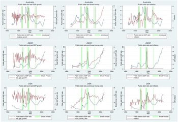
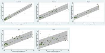
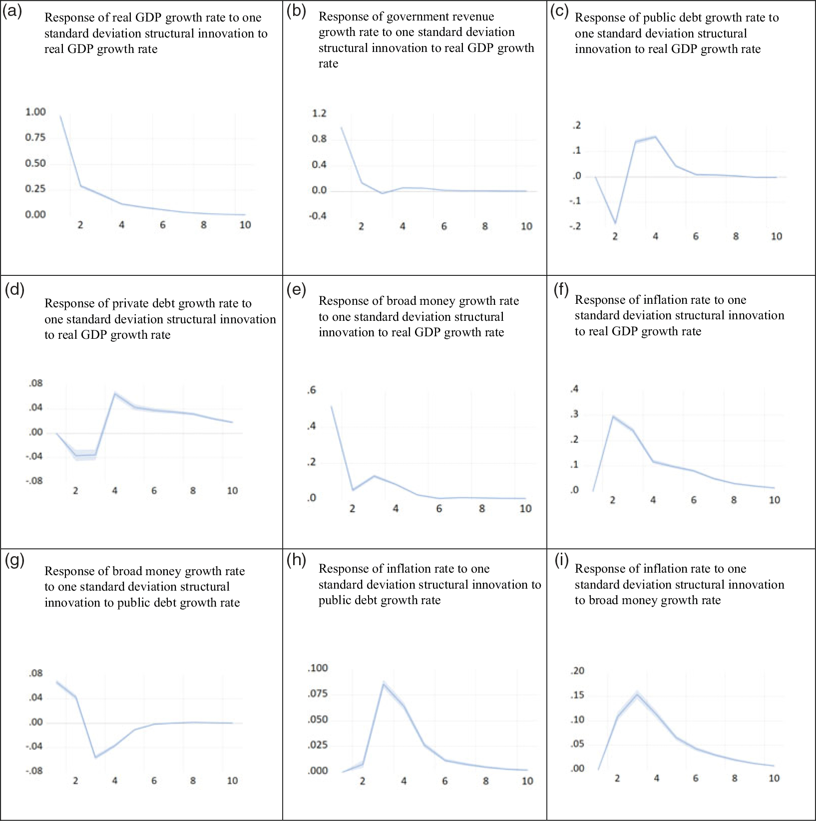
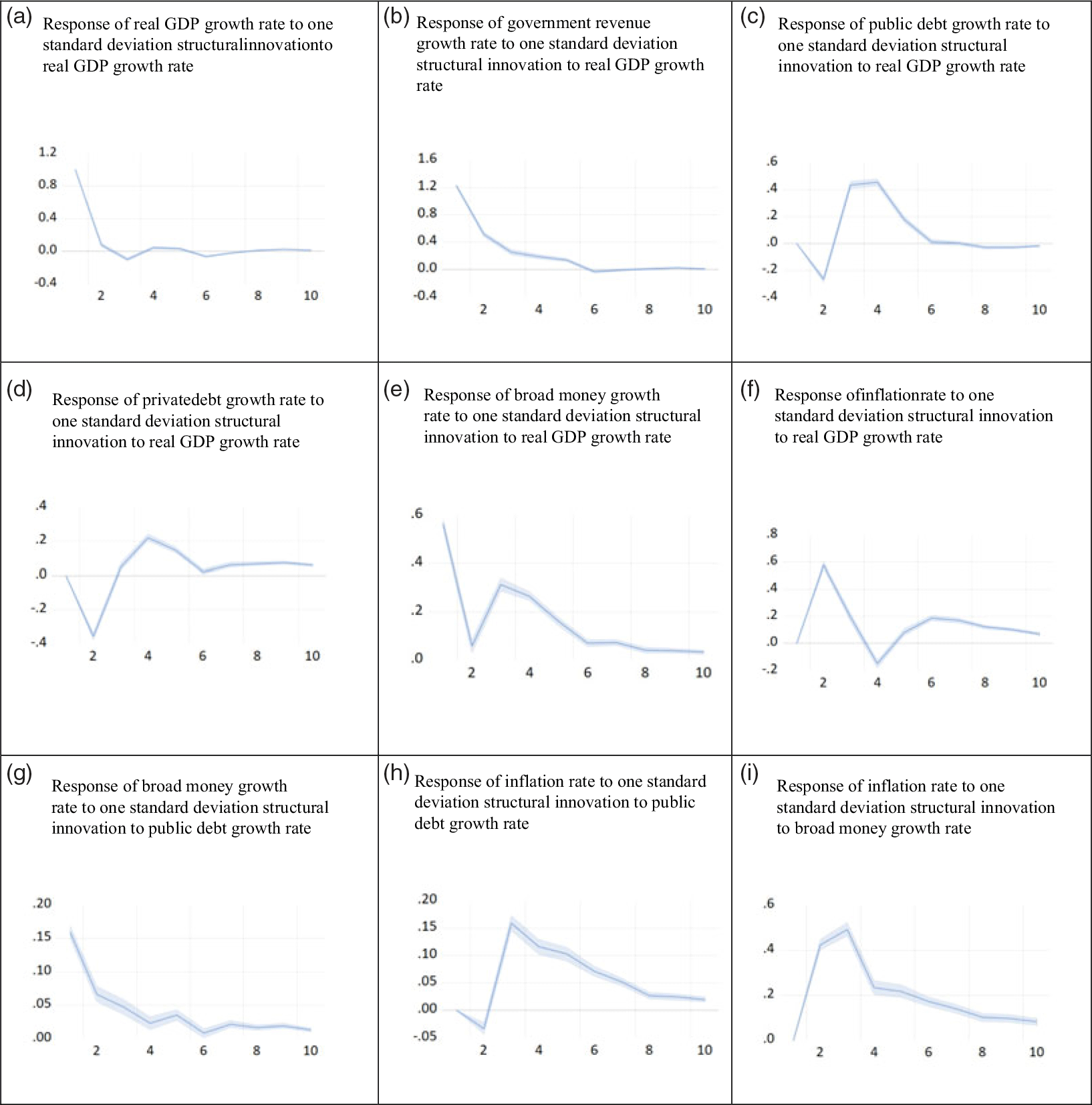
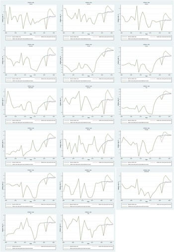


 Open access