
Introduction
The promise of electric deregulation has long eluded dinner-table conversation in the American household. However, although it is uncommon discussion fodder for residential consumers at home, electric deregulation policy is much debated by legislators and regulators. This is partly because of its potentially significant impact on consumer welfare through the effect it has on the monthly bills customers pay and the essential nature of electricity service in the modern economy. Given its importance to consumers and a recent resurgence in legislative attention to the subject, identified below, the study of the implementation and effect of electric deregulation is of renewed interest to scholars. Deregulation’s “promise” was increased efficiency and decreased retail rates to both households and businesses through the introduction of competition (Winston Reference Winston1993; Newbery Reference Newbery1999; Hunt Reference Hunt2002). These benefits have not been consistently identified in the literature evaluating deregulation of electric markets. This article provides an empirical analysis of the State of Ohio’s experience with retail electric deregulation. The unique context allows us to evaluate both the underlying theory and its implementation. We find that the divergence between the promise of deregulation and what consumers have actually observed may be less of a flaw in the underlying deregulatory theory than problems with the implementation of deregulatory policy.
The underlying theory of electric market deregulation, also known as restructuring, is based upon a long-standing literature that argues that liberalising the industry can reform some of the well-understood distortions of public utility regulation (Stigler and Friedland Reference Stigler and Friedland1962; Joskow and Schmalensee Reference Joskow and Schmalensee1983; Peltzman Reference Peltzman1989; Phillips Reference Phillips1993). A subsequent reform agenda was pursued predominantly at a wholesale level, affecting the generation and transmission of electricity and leading to the creation of restructured wholesale energy markets. Despite pushing for these changes, scholars argued that regulators should still play a fundamental role in overseeing fair and efficient retail rates for regional distribution utilities, and that deregulation should not eliminate regulatory rate-setting at the retail level (Joskow and Schmalensee Reference Joskow and Schmalensee1983; Hilke Reference Hilke2008). The “textbook” model of electric restructuring called for retail deregulation only after extensive and careful market development, as well as the functional separation of competitive and noncompetitive services (Hunt Reference Hunt2002; Joskow Reference Joskow2005a, Reference Joskow2008).
In practice, retail deregulation, or “retail choice” as it is often called, means that residential customers can either “shop” from among competing marketers to supply their generation on a contractual basisFootnote 1 or remain with the regional monopoly supplier and be charged a rate that is set by some competitive processes, such as a supply auction, detailed below. Full retail deregulation effectively divorces commission oversight from setting electric rates for everything except local distribution service. Although most states today that deregulated have done so in wholesale markets, an increasing number are fully, or at least partially, liberalising retail electricity service as well.Footnote 2
While it is tempting to simplify the issue by identifying states as either “regulated” or “deregulated”, we caution against this oversimplification. Ultimately, electric deregulation exists on a continuum that varies by the degree of commission involvement in rate-setting. Many states that introduced competition into their electricity markets still maintain some level of commission oversight, and thus prudence review, over the behaviours of regional monopoly distribution utilities. Consequently, the effect that households observe is fundamentally a product of how this underlying theory is implemented.
Today, there is a lack of definitive empirical evidence regarding how electricity restructuring has ultimately affected the welfare of businesses and households (Eto et al. Reference Eto, Hale and Lesieutre2006; Joskow Reference Joskow2008; Kwoka Reference Kwoka2008). Moreover, prior evaluations of electric restructuring’s impacts focused almost exclusively on wholesale market dynamics, such as generation efficiencies (Markiewicz et al. Reference Markiewicz, Rose and Wolfram2004; Bushnell and Wolfram Reference Bushnell and Wolfram2005; Craig and Savage Reference Craig and Savage2013; Cicala Reference Cicala2014) and wholesale prices (Green and Newbery Reference Green and Newbery1992; Chapman et al. Reference Chapman, Vossler, Mount, Barboni, Thomas and Zimmerman2004; Puller Reference Puller2007; Hortaçsu and Puller Reference Hortaçsu and Puller2008; Mansur Reference Mansur2008; Davis and Wolfram Reference Davis and Wolfram2012; Dias and Ramos Reference Dias and Ramos2014). The body of scholarship that does study the effect of retail restructuring on consumer rates is growing, but remains incomplete and is often contradictory. Apt (Reference Apt2005), using a diff-in-diff approach and looking at the rate of change in industrial prices, found that restructuring did not lead to lower prices. Fagan (Reference Fagan2006), in contrast, found that industrial prices in restructured states outperformed predicted prices using a counterfactual model. Swadley and Yücel (Reference Swadley and Yücel2011) similarly found, using a dynamic panel model, that retail competition led to lower prices. Taber et al. (Reference Taber, Chapman and Mount2006) tested a variety of model specifications and deregulation definitions and observed that consumers in deregulated states faced higher relative prices. Their research, however, did not account for retail choice. Joskow’s (Reference Joskow2006) econometric study of electric restructuring identified between a 5 and 10% decrease in real retail prices owing to both wholesale and retail restructuring. This work, however, is also limited by problems stemming from the extent of restructuring and measurements of electric prices.
The handful of more recent studies on the price effects of restructuring do not resolve the contradictions identified in the first wave of restructuring studies. Su (Reference Su2015) found that retail competition led to mixed-to-lower prices, with benefits mainly seen by residential customers. Ros (Reference Ros2017) also identified lower prices, but found the greatest and most sustained savings accruing to industrial customers with the least benefit flowing to the residential class. Intra- and interstate variation in price effects is attributed in some studies to fuel prices as mediated by utility fuel mix, although this relationship depends on the extent that restructuring mechanisms allowed greater pass-through of wholesale market costs to consumers (Borenstein and Bushnell Reference Borenstein and Bushnell2015). Although the bulk of the literature studying deregulation policy and its impact is concentrated in the 2000s, the impact of electricity market restructuring is again salient to policymakers. Several restructured states are considering reregulating energy services or introducing greater regulatory oversight to shield preferred generation resources against market forces.Footnote 3 In addition, in the intervening years since the initial studies, many markets previously considered to be “deregulated” finally implemented or completed major restructuring reforms for the first time.
The State of Ohio offers a robust opportunity for evaluating the effects of retail restructuring, as well as the relationship between these effects and policy implementation. Ohio is technically deregulated in both the wholesale and retail markets; however, important regulatory vestiges remain that have affected prices in key ways. Like many similar states, Ohio’s implementation diverged from the core textbook model of deregulation in two important ways. First, the statutory language is ambiguous on a key deregulatory design feature. Statutory ambiguity has been identified as a cause of implementation failure (Sabatier and Mazmanian Reference Sabatier and Mazmanian1980; Mazmanian and Sabatier Reference Mazmanian and Sabatier1981; Huber and Shipan Reference Huber and Shipan2002; Hill, Reference Hill2003; Zahariadis and Exadaktylos Reference Zahariadis and Exadaktylos2016). It gives agencies wide latitude in implementing statutes (Mahoney and Thelen Reference Mahoney and Thelen2010). The statutory language called only for corporate, rather than functional, separation of generation from distribution. In other words, rather than requiring utilities to divest their competitive generation assets (almost entirely legacy coal plants), the commission used their broad discretion to allow utilities to create arms-length, affiliate corporations, which retained ownership of generation assets.
Second, the statute allowed the commission to structure decision rules that permitted rent-seeking (Krueger Reference Krueger1974; Wright Reference Wright1977; Appelbaum and Katz Reference Appelbaum and Katz1987; Tullock Reference Tullock2001; Carter et al. Reference Carter, Weible, Siddiki, Brett and Chonaiew2015). The commission pursued a distribution rate-setting process that eased the procedural requirements for adding nonbypassable riders and surcharges to customers’ bills. This permitted utilities to broadly pursue cost recovery, including for their arms-length deregulated plants. The textbook model of deregulation calls for deregulated plants to recover their costs solely through the wholesale market so that customer welfare is not tied to the fortunes of a regional monopoly utility without regulatory protection. Ohio’s context uniquely allows us to compare the policy and its implementation, as one of the state’s four utilities (Duke Energy) followed a more textbook model of retail deregulation by functionally divesting its generation assets. It thus had no instrumental interest to recover generation-related costs by adding riders to electric bills.
The case of Ohio also uniquely allows us to assess retail restructuring because the state maintains accurate residential final bill data that provide far more detailed information than the data source typically used in competing studies – Energy Information Administration (EIA) data. EIA data do not include revenues obtained through riders and surcharges. In addition, the transition towards market-based retail rates and more limited commission rate-setting was sudden, allowing for a robust quasi-experimental evaluation with a clean cut/intervention point to provide for a pre- and post-assessment.
We begin by providing a concise case history of electric restructuring in Ohio to provide both context for our empirical work and to elucidate the specific market design and implementation path pursued. We then describe the data we utilise and general trends in the costs customers have faced. From this, we provide the results of quasi-experimental analyses for the seven largest indicative metro areas, or service territories, in Ohio, representing the majority of the state and excluding only rural coops, municipal power and municipal aggregators.Footnote 4 We provide estimates of the impacts of retail market restructuring on residential electricity bills. We also provide welfare impact estimates for these territories. We conclude with insights for the current reregulation debate, and policy implementation more broadly.
The case of restructuring in Ohio
Before restructuring, Ohio’s predominant electric utility model relied on vertically integrated monopolies. These monopolies oversaw all aspects of electricity provision: generation, transmission and distribution (T&D) and retail services. These utilities were overseen by the Public Utilities Commission of Ohio (PUCO) and subject to price and cost regulation, consisting of the cost of operation plus a return on “used and useful” capital investment (Shapiro and Tomain Reference Shapiro and Tomain2003). Four investor-owned utilities (IOUs) – FirstEnergy, American Electric Power (AEP), Duke Energy and Dayton Power & Light (DP&L) – provided nearly 90% of electric market services in 1999.Footnote 5 Under regulation, PUCO attempted to balance consumer and utility interests through traditional ratemaking proceedings, including systematic review of rate components.
Ohio, like many peer states, faced a political climate favourable to electric restructuring in the 1990s, particularly at a wholesale market level. At this time, low natural gas prices relative to alternative fuels contributed to low marginal costs in liberalised wholesale markets. The Federal Energy Regulatory Commission (FERC) put forth rules for nondiscriminatory access to wholesale power markets with FERC Order 888 in 1996, essentially opening up these markets. This order installed independent system operators (ISOs), run by impartial dispatchers, to oversee the flow of generated electricity across transmission networks, as opposed to local utilities (Hogan Reference Hogan1998; Hunt Reference Hunt2002; Joskow Reference Joskow2005b; Pollitt Reference Pollitt2012). FERC later refined the ISO concept with FERC Order 2000 in 1999, tasking newly created regional transmission organisations (RTOs) to manage wholesale market design and administration (Chandley Reference Chandley2001; Hunt Reference Hunt2002; Joskow Reference Joskow2005b).
As an added incentive to reform, Ohio utilities charged customers high average costs under the traditional monopoly system. Although the average utility retail price of 9.09 cents/kWh (2014 dollars)Footnote 6 in 1999 was only 22nd highest out of the 50 United States’ states, Ohio’s electric consumption, led by a large industrial sector, was the fourth highest in the country (EIA 2001). Given the prospect of accessing cheaper wholesale electricity, some industrial and commercial interest groups intensely lobbied in support of wholesale restructuring. Proponents argued that deregulation would lead to welfare gains for all involved parties.
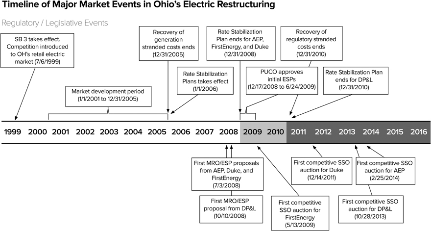
Ohio initiated its effort to deregulate by passing Senate Bill (SB) 3 in June 1999. One of the stated goals of SB 3 was to reduce costs and increase choice for all customers. Consequently, SB 3 established a path towards retail restructuring in addition to wholesale reforms. A timeline of major events in the history of Ohio electric restructuring starting with SB 3 is included in Figure 1, and specific dates are listed in Appendix Table A.1. SB 3 established 1 January 2001 as the starting date of competitive retail electric service and unbundled electric services to allow customers the ability to “shop” for a retailer of choice, known as competitive retail electric suppliers (CRES).Footnote 7 SB 3 also established a five-year Market Development Period during which time incumbent utilities could collect market transition revenues (i.e. stranded costs) either through a rate freeze with specified adjustments or transition charges paid by customers who switched supply [Ohio Legislative Service Commission (OLSC) 1999].
Timeline of major market events in Ohio’s electric restructuring. Note: SB=Senate Bill; AEP=American Electric Power; PUCO=Public Utilities Commission of Ohio; ESP=Electric Security Plan; DP&L=Dayton Power & Light; MRO=Market Rate Offer; SSO=standard service offer. Source: authors.
A law declaring the existence of a market does not necessarily mean that the market will materialise. In Ohio’s case, instead of first developing an adequate retail market, the restructuring process started with efforts to subsidise switching.Footnote 8 This approach was ill-advised, as switching incentives had no basis in actual market price, little progress had been made to reduce market concentration or create firewalls between regulated utilities and deregulated subsidiaries and few rules of conduct existed for CRES. These supply-side flaws caused issues related to market power, gaming and inefficiency that all deterred suppliers from participating in the retail market (Hunt Reference Hunt2002). Unsurprisingly, a competitive retail electric market did not develop as envisioned by the proponents of SB 3.Footnote 9 The PUCO, observing this situation, adopted the rhetoric used by utilities that a clean change to market-based rates would lead to “rate ‘sticker shock’” (PUCO 2007). It is important to note that utilities had a financial interest in maintaining regulated rates as it allowed them to continue earning guaranteed, regulated returns on generation assets.
Instead of concluding market development, the PUCO opted to delay its end with the backing of the Ohio Legislature. Between October 2002 and January 2005, the PUCO approved individually negotiated Rate Stabilization Plans (RSPs) – a continuation of regulated ratemaking and elements of market development – with all four major Ohio IOUs.Footnote 10 During this period, utilities sought additional returns as a means to further recover stranded costs before open wholesale market competition. Although the recovery of generation stranded costs statutorily ended 31 December 2005, RSPs allowed FirstEnergy, AEP, and Duke Energy to continue receiving regulated rates that included transition cost recovery until 31 December 2008, and DP&L until 31 December 2010.Footnote 11 These dates thus become the key policy intervention dates for our quasi-experimental estimation as these dates identify the end of comprehensive commission rate-setting.
Of critical importance to Ohio’s restructuring process was the fact that SB 3, although it instructed incumbent utilities to unbundle, did not unambiguously specify a requirement for functional separation (i.e. divesture) of competitive assets, including generation. Rather, it required that utilities “corporately separate”. By requiring each utility to develop a corporate separation plan, the statute was sufficiently ambiguous that the PUCO could permit utilities to technically unbundle by divesting their generation assets to an arms-length corporation owned by the same parent corporation. For example, the PUCO approved a corporate separation plan for AEP Ohio that allowed it to sell its generation (a legacy coal fleet) to the newly created AEP Generation Resources, LLC, owned by AEP Ohio’s parent corporation. Similar arms-length firms were created by FirstEnergy and DP&L.
The provisional status of Ohio’s electric restructuring was clarified with the passage of SB 221 in May 2008. SB 221 required that Ohio’s incumbent utilities obtain PUCO approval for either a Market Rate Offer (MRO) or an Electric Security Plan (ESP) to fulfil their standard service offer (SSO), or default service, obligations by the end of the aforementioned RSP period. The legislation also specified that these plans “exclude any previously authorised allowances for transition costs” (OLSC 2008). MROs represent a purer market-based rate-setting process in which the prevailing SSO rates are set by “competitive bidding process (CBP)” (OLSC 2008) auctions that tie generation pricing to actual wholesale market prices.Footnote 12 ESPs utilise CBP auctions as well, but additionally allow for what energy attorneys refer to as “single-issue ratemaking”.Footnote 13 ESPs enable utilities to propose nonbypassable riders, which must be approved as a package in a single up or down vote by commissioners. Because ESP riders are not bypassable, their costs are incurred by all consumers regardless of whether they have switched to a marketer or remain on the SSO rate. Although MROs were the legislative default, utilities prefer ESPs because they greatly reduce the burden of obtaining additional revenue streams from consumers.
Under the rules of SB 221, utilities were required to simply demonstrate that ESP pricing was “more favourable in the aggregate as compared with the expected results that would otherwise apply under an MRO” (OLSC 2008). This became known as the “ESP versus MRO test”. Because this test was unusually broad as compared with regulated ratemaking processes, all utilities obtained ESPs. Counter to the intentions of the legislature, to date, no MROs have been implemented. Utilities have no incentive to move to MROs, and thus lose the ability to obtain riders and surcharges. The existing ESP plans in effect for all four major IOUs include nearly three dozen additional nonbypassable riders. In addition, SB 221 did not substantively address divestiture or corporate separation, allowing incumbent utilities to continue arms-length ownership of generation.
SB 221 set in motion the competitive provision of electric services.Footnote 14 Regulators believed that ESP plans allowed utilities “to ‘ramp up’ to market and operate under a blended generation price” (OLSC 2008) until an eventual MRO proposal. A PUCO staff investigation into the state of Ohio’s retail electricity market between December 2012 and January 2014 argued that Ohio’s hybrid form of restructuring achieved “effective competition” (PUCO 2012).Footnote 15 The implementation of Ohio’s retail restructuring (SB 221) is the most appropriate policy intervention point for this study. With SB 221’s implementation, the state observed the end of regulatory rate review for pricing generation and the true opening of competitive retail choice, but also the beginning of nonbypassable riders and surcharges issued through single-issue ratemaking. The latter provided a means to circumvent the important deregulatory objective of unbundling.
Data
Survey data
The PUCO provides a monthly publication of utility rates in each utility service territory in Ohio conducted as part of its market evaluation and oversight function. These Ohio Utility Rate Surveys comprise the main source of data for this analysis. The surveys provide total electric bill charges for fixed consumption levels by customer class (i.e. residential, commercial and industrial). We note that in this article we focus solely on residential rates, which are the predominant focus of retail restructuring. The fact that the survey data include total bill information for fixed consumption levels is important to this study for three reasons.
First, total bill information is not commonly used in other analyses. The data source relied on for most studies to date has been EIA data (e.g. EIA 826), which provides an incomplete estimate of the marginal rate that customers pay for their electricity (i.e. cents/kWh) based on aggregate sales revenue reports of the distribution utility and excluding revenues obtained by riders and surcharges.Footnote 16 Consequently, because this study uses actual customer final bill data, it relies on a more accurate representation of the actual costs incurred by households, including riders and surcharges that flow through to arms-length subsidiaries. Second, the data provide total bills for fixed consumption levels on a monthly basis. This is important, particularly given the quasi-experimental approach we use, because the data already inherently control for consumption and seasonal variation in demand for electricity.Footnote 17 All of the electricity data reported in the surveys provide total bill costs for customers using 750 kWh. In this way, the surveys are not “surveys” as the term is typically used, but rather reflect what the commission views as a “typical bill” that is representative of a typical household.Footnote 18
Third, the data are also helpful because they account for heterogeneity in tariff pricing structures across utilities and across time. That is, some utilities have pricing structures for some or all of their customers that utilise stepwise (also called “tiered”) pricing rather than fixed rates. Under tiered pricing, utilities can charge higher marginal rates for higher consumption levels. Using fixed rate survey data eliminates the problem of accounting for differences in tiers between utilities and over time.
The surveys provide data only for SSO customers. CRES rates are contractual and based on the marketers’ costs of procuring supply from the RTO. As such, there is heterogeneity across supply offers, in terms of both marginal rate and supplemental services offered (e.g. higher renewable percentages, longer-term fixed rate lock-ins). The fact that this study evaluates total customer costs based on SSO rates does not limit the explanatory power of our analysis. This is for two reasons. First, the SSO is by far the prevailing rate in Ohio’s retail market throughout the time period studied. Appendix Table A.2 provides indicative counts of utility customers served by the default offer over time. As this table shows, the majority of residential customers served by major utilities – approximately 57%, or 2.7 million customers – faced the SSO rate as recently as December 2015. The proportion of switched customers has plateaued over time. This is consistent with prior literature that has found that large subsets of residential customers are subject to inertia in restructured markets (Giulietti et al. Reference Giulietti, Price and Waterson2005; Brennan Reference Brennan2007; Gamble et al. Reference Gamble, Juliusson and Gärling2009; Yang Reference Yang2014; Hortaçsu et al. Reference Hortaçsu, Madanizadeh and Puller2017).
Second, customers who switch to a CRES supplier can only obtain a different price for the generation component of their bill. All of the other costs, inclusive of riders, as well as regulated T&D, are nonbypassable, leaving the lion’s share of the bill unchanged. In addition, the generation price for SSO and CRES customers should converge over time because both CRES and SSO rates are priced from the same wholesale market. Consequently, SSO rate data, as used here, are representative of the effects observed by all residential customers.
Data summary and general trends
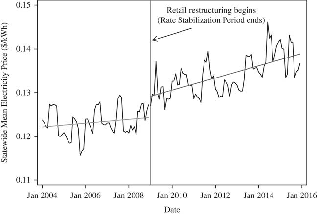
The data span the years 2004 through 2015. In total, we use 144 monthly observations for each metro area. Table 1 below provides simple summary statistics in marginal rates ($/kWh) that reflect the entirety of the bill that customers receive. This is an important distinction because utilities report to customers a lower marginal rate that only accounts for the generation costs. Bills for these customers averaged between 11 and 13 cents/kWh. They ranged between 8 cents and over 18 cents/kWh. Whereas Table 1 provides summary statistics within each of the major metro areas, we also provide the average by month across all of the metro areas to give a statewide aggregate electricity price. We show this as a time series plot in Figure 2. All time series data are adjusted by the general consumer price index to correct for inflation, and all values are reported in real 2014 dollars.Footnote 19
Statewide aggregate electricity price. Note: Values reflect the mean, inflation-adjusted marginal rate for all utility service territories excluding Dayton Power & Light (which restructured two years later).
Average total electricity bills (2004–2015)
Note: The values provided are marginal rates ($/kWh) for the entirety of the electricity bill, inclusive of riders and surcharges. All values are in constant 2014 dollars.
It is clear that there is a general upward trend after retail restructuring and that it did not, in general, lower rates or keep rates constant. Whereas the mean statewide aggregate electricity price before restructuring was 12.63 cents/kWh, it was 13.29 cents following restructuring. Figure 2 excludes Dayton as it implemented restructuring two years later.
Method of analysis
Interrupted time series (ITS) models
We use an ITS design to evaluate the implementation of retail restructuring on default electricity prices (i.e. SSO price). ITS is a strong empirical approach for this particular application because it removes the time series pattern of data to provide an unbiased comparison of the pre- and post-retail restructuring periods given that electricity prices are measured at regular monthly intervals (Campbell and Stanley Reference Campbell and Stanley1963; Abadie and Gardeazabal Reference Abadie and Gardeazabal1999; Shadish et al. Reference Shadish, Cook and Campbell2002). In addition, as provided in the second section, ITS is contextually appropriate because the implementation of restructuring in Ohio provides for a clean policy intervention point (i.e. the implementation of SB 221) at which point traditional cost-of-service regulation for pricing generation ended.
Our null hypothesis is that the retail electricity price will have declined following the introduction of a market-basis for rate-setting, as purported by proponents of restructuring. Such changes can take two forms: a change in intercept (i.e. a change in the average electricity price after retail restructuring) or a change in slope (i.e. a change in the trend of electricity price after retail restructuring).
The general functional form of our model is given by:%
 $$\eqalignno{ Price_{t} \,{\equals}\,\alpha {\plus}\beta _{1} \left( {Month_{t} } \right){\plus}\beta _{2} \left( {{\it Post{\hbox \-}restructuring}} \right){\plus}\beta _{3} \left( {Month_{t} } \right)\left( {{\it Post{\hbox \-}restructuring}} \right)\cr \hskip35pt{\plus}{\varepsilon}_{t} $$
Price t provides our explanatory variable of interest, electricity price in a given month t. Month t is a month index beginning with our first available month of data, January 2004. The coefficient β 1 provides the general month-to-month price trend ignoring any intervention (i.e. the trend before retail restructuring). Post-restructuring is a dummy variable that provides the “interruption” of the series (i.e. our policy intervention point). Post-restructuring takes a value of “0” for months before restructuring, and a “1” for subsequent months during restructuring. The coefficient β 2 provides the change in the intercept of the electricity price trend after retail restructuring began. The coefficient β 3 of the interaction term (Month t ) (Post-restructuring) provides the change in the month-to-month price trend between the pre-restructuring period and the restructuring period. Thus, it provides the difference in the slopes of the two trend lines (post-policy minus pre-policy).
The coefficient of the interaction term, β 3, could indicate a number of possible policy effects. For example, for any given model, if the coefficient is negative (and statistically significant), this indicates that restructuring had the effect of decreasing the pre-restructuring price trend for a given utility. We also note that a positive and significant β 3 would indicate the opposite effect, namely that the post-intervention monthly trend increased relative to before restructuring for all the same scenarios but in the opposite direction.
In addition, we note that lack of statistical significance of β 3 does not necessarily indicate a null finding. Lack of statistical significance of this coefficient should be taken, as a whole, in consideration with β 1 (which is the pre-restructuring trend). Proponents of retail restructuring argued that competitive retail markets would bring rates down. A positive and significant β 1 would indicate, for example, that prices were on the rise before retail restructuring. A nonsignificant β 3 would therefore indicate that restructuring did not have its intended effect, and that rates continued to rise after restructuring just as they had been rising on a monthly basis before.
The main modelling approach for accounting for this time series is the autoregressive integrated moving average (ARIMA) approach, which allows us to retain the controlled pre- and post-treatment effect measures while accounting for autocorrelation (Box and Jenkins Reference Box and Jenkins1970; Hamilton Reference Hamilton1994; Box-Steffensmeier et al. Reference Box-Steffensmeier, Freeman, Hitt and Pevehouse2014; Enders Reference Enders2014). Properly correcting for autocorrelation is both theoretically and contextually important with this data, as household electricity prices in a given month tend to be highly correlated with prices in prior months. The structure of an ARIMA (1, 0, 0) model is given by:%
 $$\hskip-35pt \eqalignno{ (1{\hbox \-}\hskip0.5pt \Oslash \varnothing _{1} \hskip-2pt B)\,Price_{t}\;{\equals}\;\alpha {\plus}\beta _{1} \left( {Month_{t} } \right){\plus}\beta _{2} \left( {{\it Post{\hbox \-}restructuring}} \right)\cr \hskip69pt{\plus}\beta _{3} \left( {Month_{t} } \right)\left( {{\it Post{\hbox \-}restructuring}} \right){\plus}{\varepsilon}_{t} $$
Building upon model (1), model (2) adds (1-Ø1 B) that indicates the autoregressive (AR) (1) process. B is a backshift operator.
However, the data for some cities exhibit a fractionally integrated process. These cities are Canton, Columbus, Cincinnati and Dayton. First-differencing the data would lead to over-differencing based on the autocorrelation function (ACF) and partial autocorrelation function (PACF) plots. The fractional integration process has the characteristics of both unit root and stationarity. Similar to a stationary process, fractionally-integrated time series are mean reverting in the long run. In addition, similar to an integrated process (e.g. unit root), fractionally-integrated time series will exhibit strong dependence between observations over time. It has been argued that treating fractional integration as either unit root or stationary will threaten the validity of any statistical inferences (Sowell Reference Sowell1992; Baillie Reference Baillie1996; Box-Steffensmeier and Smith Reference Box-Steffensmeier and Smith1998). Thus, we use an autoregressive fractional integrated moving average (ARFIMA) model that allows the integrated order (d) to take noninteger values (i.e. fractions).
The selection of AR and MA orders are based on the diagnosis of the characteristics of electricity price data for given utility service areas, which will be discussed later in more detail. Generally, the time series for the utility service areas associated with fractional integration can be best fit into the ARFMA (1, 0, 0) model, as given by:%
 $$\hskip-25pt \eqalignno{ \left( {1{\hbox \-}B} \right)^{{\rm d}} (1{\hbox \-}\hskip1.5pt\Oslash\varnothing _{1} \hskip-2pt B)Price_{t}\;{\equals}\;\alpha {\plus}\beta _{1} \left( {Month_{t} } \right){\plus}\beta _{2} \left( {{\it Post{\hbox \-}restructuring}} \right)\cr \hskip93pt{\plus}\beta _{3} \left( {Month_{t} } \right)\left( {{\it Post{\hbox \-}restructuring}} \right){\plus}{\varepsilon}_{t} $$
Building upon model (2), model (3) adds one variable: the estimate of fractional integration (d). Our hypothesis suggests that electricity prices should ceteris paribus decrease after restructuring for one of the above-mentioned four scenarios. Therefore, we expect the coefficient of the interaction term (β 3) to be negative, which means restructuring has a negative impact on the fractionally-differenced electricity price.
For some service areas, we use a seasonal autoregressive integrated moving average (SARIMA) model to handle the added complexity of seasonality. These cities are Akron, Cleveland and Toledo. The SARIMA model is often denoted as an ARIMA (p, d, q)×(P, D, Q)s. On the basis of the diagnosis details that are discussed later, the electricity data for utility service areas with significant seasonality can be best estimated by the ARIMA (1, 0, 0)×(1, 0, 0)12, given by:%
 $$\hskip-12pt \eqalignno{ (1{\hbox \-}\hskip1.5pt\Oslash\varnothing _{1} \hskip-2pt B)\,\left( {1{\hbox \-}\Phi _{1} B^{{12}} } \right)Price_{t}\;{\equals}\;\alpha {\plus}\beta _{1} \left( {Month_{t} } \right){\plus}\beta _{2} \left( {{\it Post{\hbox \-}restructuring}} \right)\cr \hskip113pt{\plus}\beta _{3} \left( {Month_{t} } \right)\left( {{\it Post{\hbox \-}restructuring}} \right){\plus}{\varepsilon}_{t} $$
Model (3) adds the seasonal AR (1) component (1-Φ1 B 12) and the AR (1) component (1-Ø1 B) to model (2). Similar to models (2) and (3), a negative coefficient of the interaction term (β 3) would support the conclusion that restructuring lowered retail electricity prices.
Model selection
Our approach to model selection began with diagnosing the time series properties of the electricity price data for each utility service area; this is consistent with the long-standing approach taken by Box and Jenkins (Reference Box and Jenkins1970). We first used the generalised Box-Jenkins approach of reviewing the ACF plots and PACF plots for each city to examine whether electricity prices exhibit unit root and seasonality (see Appendix Figure A.1). Electricity prices in Canton, Cincinnati, Columbus and Dayton have significant spikes even after 10 lags. Such patterns suggest that the data for those territories probably exhibit a unit root. Moreover, the periodic spikes around every 12 intervals (months) suggest that electricity prices in Akron, Cleveland and Toledo exhibit yearly seasonality. We note that the main utility provider for these cities is FirstEnergy.
Correlograms of electricity prices. (a) Akron, (b) Canton, (c) Cincinnati, (d) Cleveland, (e) Columbus, (f) Dayton and (g) Toledo
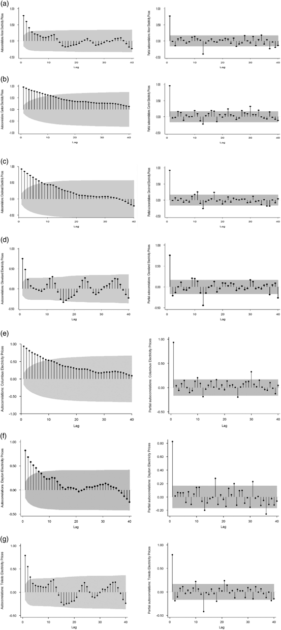
Second, we use two formalised tests to complement the evidence obtained from the visual diagnosis of stationarity: the widely used Dickey-Fuller test and Variance Ratio Test (Dickey and Fuller Reference Dickey and Fuller1974; Lo and MacKinlay Reference Lo and MacKinlay1988). Appendix Table A.3 provides the results of Dickey-Fuller tests (including time trend). We fail to reject the null hypothesis that electricity prices in Canton, Cincinnati, Columbus and Dayton exhibit unit root behaviour with trend. The Dickey-Fuller test results are consistent with our visual diagnosis.
However, some scholars argue that the Dickey-Fuller test has less definitive power, which means that we may too easily accept that we have a unit root for those territories in the face of fractional integration (Box-Steffensmeier et al. Reference Box-Steffensmeier, Freeman, Hitt and Pevehouse2014). To compensate for that potential weakness in the Dickey-Fuller test, we also run variance ratio tests for which the null hypothesis is a unit root (the integrated order d=1). The alternative hypothesis suggests that either a fractional integration or stationarity (d<1) is appropriate. Appendix Table A.4 presents the results of the variance ratio tests for various choices of the differencing interval (2, 4, 8 and 16 months). As the results suggest, the null hypothesis that the series has a unit root can be rejected for Toledo at all differencing intervals. We fail to reject the null hypothesis of a unit root for Cincinnati and Columbus at all differencing intervals. For the other four cities (Akron, Canton, Cleveland and Dayton), the variance ratio tests reject the null hypothesis at some differencing intervals. This implies that the series are probably fractionally integrated.
Finally, the hyperbolic decay in the ACF and a significant spike at the first lag in the PACF suggest that the electricity prices in all cities exhibit an AR (1) process. For Akron, Cleveland and Toledo, we also detect a seasonal AR (1) component in the corresponding PACF plots as the spikes around the 12th lag are significant.Footnote 20
On the basis of the diagnostic results and the performance of multiple competing models on the post-estimation tests (e.g. nonlinearity tests, white noise tests and information criterion), we identify the strongest model fit for Akron and Toledo to be an ARIMA (1, 0, 0)×(1, 0, 0)12 model, and an ARIMA (2, 0, 0)×(1, 0, 0)12 to best fit Cleveland. Similarly, we identify the strongest model for Cincinnati, Columbus and Dayton to be an ARFIMA (1, 0, 0) model. Finally, we identify the strongest model for Canton to be an ARIMA (1, 0, 0) model given that the ARIMA (1, 0, 0) has almost equal performance on the post-estimation tests as a more complicated ARFIMA (1, 0, 0) suggested by the diagnostic results, but with a higher degree of parsimony.
We conduct Enders’ Regression Equation Specification Error Test (RESET) to identify any nonlinearity in the pre- versus post-policy intervention data (Appendix Table A.5) for the specified models. The test results reject significant structural changes in the electricity price data for all seven metro areas. We also provide Portmanteau and Bartlett’s white noise test statistics (Q and B statistics, with accompanying p-values) of each preferred model for the period preceding regulatory restructuring, the period following and for the full series (Appendix Table A.6). In all cases, the data fail to reject the null (of white noise) at least at the 0.05 level or higher, indicating that there is no unobserved heterogeneity bias in the residuals. The two most marginal cases are the pre-restructuring period for Canton and the post-restructuring period for Cleveland, which marginally pass at 0.05 on only a single test, but pass handily on the other test, respectively.Footnote 21 The white-noise residuals across both the pre- and post-restructuring periods provide robust evidence of the absence of structural breaks, as the same autoregressive process fits the data for both periods.
Empirical results
Price trend summary
While proponents of market-based rate-setting of retail electric service have argued that converting regulated rates to market-based rates will reduce them, the results of our analyses provide little confirmation – and, in some cases, provide a direct refutation – of that claim. While in Figure 2 we provide the aggregate statewide time series plot of electricity prices, in Figure 3 we provide this for each of the seven major metro areas/utility service areas in Ohio, in Figure 3a–3g.
Interrupted time series plots. (a) Akron, (b) Canton, (c) Cincinnati, (d) Cleveland, (e) Columbus, (f) Dayton and (g) Toledo.
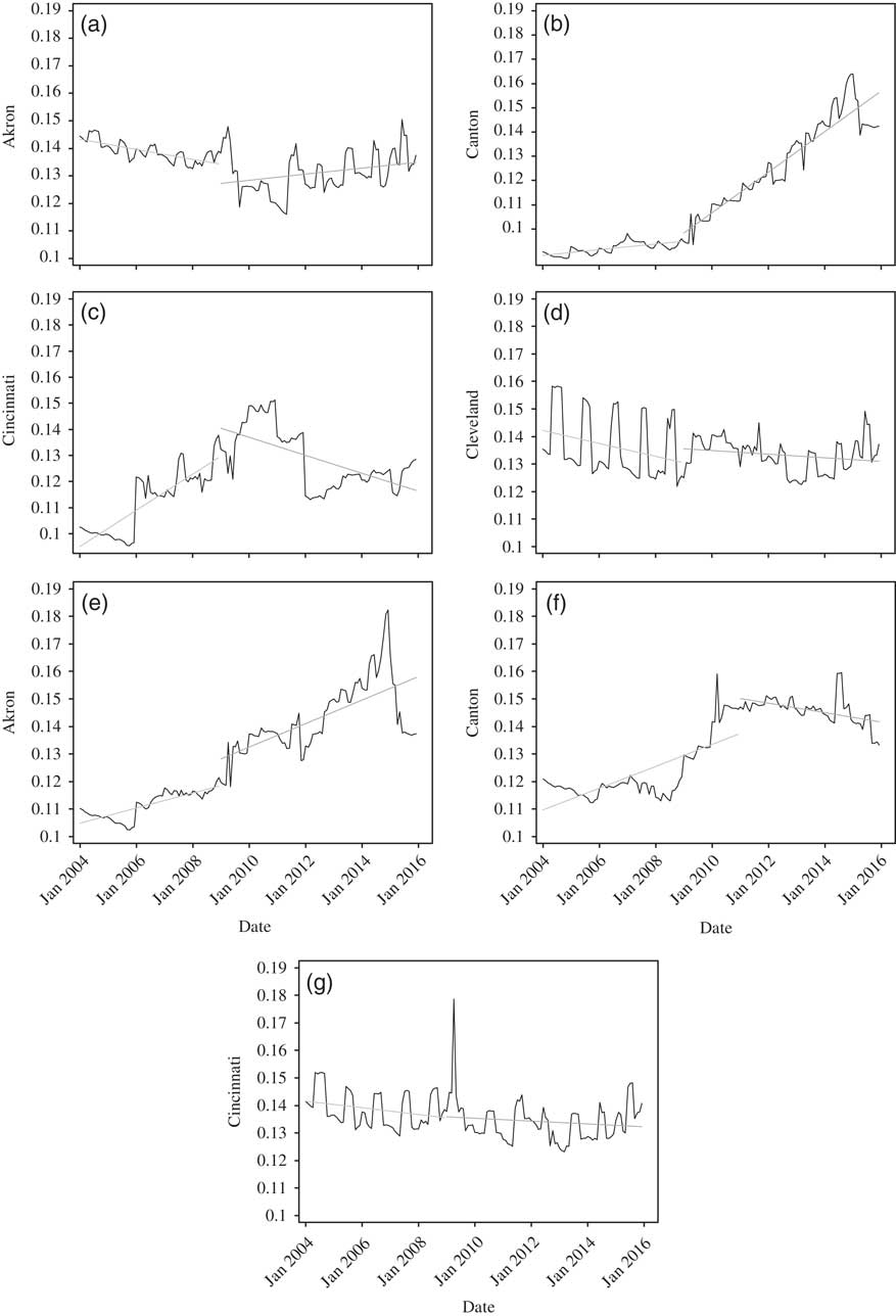
The data suggest that Akron, Cleveland and Toledo were experiencing downward trending electricity prices before the implementation of SB 221. Although Cleveland and Toledo experienced a decrease or cessation of that downward trend after implementation, Akron experienced a direct reversal. For Akron, the pre-restructuring downward trend in electricity bills became an upward trend. Canton, on the other hand, experienced a slight upward (if not flat) trend before retail restructuring that was turned abruptly and significantly upwards thereafter. The capital city of Columbus was experiencing a steady increasing trend in electricity prices before retail restructuring and that trend continued at essentially the same rate thereafter. In addition, although the post-restructuring prices there maintained a similar trend, the average prices are higher than the prices that would have resulted had the prior trend continued.
Cincinnati and Dayton differ from the rest of the state. Both Cincinnati and Dayton were experiencing increasing trends in electricity prices before retail restructuring. The pre-restructuring increasing trends were altered, and turned clearly and abruptly downwards for Cincinnati. Post-retail restructuring prices in both metro areas exhibited higher average prices than before retail restructuring.
Interrupted time series regression results
In Table 2, we provide the results of our time series models. The models have relatively strong fitness and summary measures as indicated by the Akaike Information Criterion (AIC) and Bayesian Information Criterion (BIC) statistics, indicating strong predictive power of the models overall. All model coefficients reported are in cents per kWh. Recalling that the coefficients for “Month” indicate the pre-retail restructuring price trend, we see that the coefficients all align quite closely with visual inspection of the times series plots. This coefficient is statistically significant at the 10% level for all metro areas with the exceptions of Cleveland and Toledo, which come close to statistical significance but exhibit strong seasonal variation that inflates the standard errors on even the most robust linear fit. The statistical significance of model fitness for the pre-restructuring time period gives us strong confidence in our difference (i.e. policy) measure, the interaction term, which we discuss next.
Regression results
Note: All models are Box-Jenkins autoregressive integrated moving average (ARIMA), autoregressive fractional integrated moving average (ARFIMA) or seasonal autoregressive integrated moving average (SARIMA) and use the robust estimator of variance. n=144 months.
Standard errors in parentheses *** p<0.01, ** p<0.05, * p<0.1.
The policy effect is provided in the interaction term. The interaction term, indicated by “Post 2009×Month”, is generally robust and similarly confirmed by visual inspection of the time series plots. Recall that the magnitude of the coefficient indicates the difference between the pre- and post-restructuring trends. In addition, recall that the statistical significance of that coefficient indicates the degree to which we can reject the null of pre-post price trend equality. This is important because lack of statistical significance of this coefficient does not indicate that the time series model does not fit the post-restructuring data in a robust manner; it indicates that there is no statistical difference between the slopes of the two trend lines. See Columbus, for example. Prices were rising on a monthly basis before retail restructuring in that service territory and continued to rise thereafter. The lack of statistical significance of the interaction term indicates that retail restructuring had no statistically significant effect on reducing the rising costs of electricity as purported – they continued to rise in Columbus.
For the FirstEnergy territory (Akron, Cleveland and Toledo), we see consistent decreasing prices before retail restructuring. Cleveland and Toledo continued to experience decreasing prices following retail restructuring but at a decreasing (prices falling less quickly) rate. For those two cities, we fail to reject the null that retail restructuring had an effect. For Akron, as mentioned above, we see a direct reversal in price trend that is statistically significant; an average monthly policy effect of increasing prices by 0.0275 cents/kWh. The post-retail restructuring price trend in Akron is 0.0064 cents/kWh (i.e. the pre-policy trend of −0.0211 cents plus the change/interaction term of 0.0275 cents). For residents in the Akron area who use an average of 750 kWh of electricity each month, the effect of retail restructuring translates to monthly increases in bills of approximately 21 cents above what would have been expected had the robust pre-retail restructuring trend gone uninterrupted.
For the AEP service territory (Canton and Columbus), the pre-retail restructuring trends in electric prices were a statistically significant monthly increase of 0.0138 and 0.0349 cents/kWh, respectively. The post-retail electric restructuring price trend for those cities has been 0.0692 and 0.0344 cents/kWh, respectively. As also indicated by the time series plots, Canton (formerly the Ohio Power service area) experienced a significant monthly price increase of 0.0554 cents/kWh, which is both large in magnitude and highly statistically significant. Columbus experienced no statistically significant policy effect; prices continued to rise after restructuring as they had been rising before restructuring. For residents in the Canton area who use an average of 750 kWh of electricity each month, the effect of retail restructuring translates to monthly increases in bills of approximately 41.55 cents above what would have been expected had the robust pre-retail restructuring trend gone uninterrupted.
For the Duke Energy service territory in the Cincinnati metro area, as well as for the DP&L service territory in the Dayton area, the data indicate a more favourable effect. For both areas, the data suggest that the pre-retail restructuring trend of electric prices increasing by 0.0689 cents/kWh each month has effectively been reversed. The effect of retail restructuring has been a monthly decline of over 0.081 and 0.046 cents/kWh for Cincinnati and Dayton, respectively. The post-restructuring monthly price trend in Cincinnati has been a monthly decline of 0.0124 (−0.0813+0.0689) cents/kWh. For Dayton this figure is a 0.0096 cents/kWh decline. For residents in the Cincinnati area who use an average of 750 kWh of electricity each month, the effect of retail restructuring translates to monthly decreases in bills of approximately 60.98 cents below what would have been expected had the robust pre-retail restructuring trend gone uninterrupted. For the Dayton area this figure is an average monthly price decrease of approximately 34.4 cents.
One complicating factor in interpreting these results is the intercept term associated with the post-policy trend line. For several of the areas in our study, the policy change point at which retail restructuring was implemented is given by a change in the intercept term. For example, the monthly declines in Dayton’s prices after retail restructuring do not necessarily mean that residents in the Dayton area are paying less on average for their electricity in real terms. We therefore provide the change in the intercept for each city in our regression outputs in Table 2, which is the coefficient on the policy intervention dummy variable. This change represents the difference between the y-intercept of the pre-restructuring trend and the y-intercept of the post-restructuring trend (at the beginning month of our sample, January 2004). Accounting for this, we see a downward (post-policy) change for Akron, and an upward change for Canton, Cincinnati, Cleveland, Columbus and Dayton. Moreover, we provide further insight by calculating the monthly pre- and post-policy averages in constant cents in Table 3. We note that both of the cities that exhibit downward (i.e. favourable) reversals in electric price trends (Dayton and Cincinnati) have been paying more in real terms for each kWh of electricity after retail restructuring, accounting for the post-policy intercept.
Pre- and post-retail restructuring mean monthly electric prices by metro area
Note: Values represent the average of monthly values across all months in our sample. All values are in constant 2014 cents/kWh.
Welfare effects
We extend our price impact analysis one step further by estimating welfare impacts for each of our seven metro areas and the state as a whole. By welfare, we mean the cumulative net total out-of-pocket expenditure differential of all residents in the seven major utility service areas that have electric service through their distribution utility (i.e. SSO customers) in the time since retail restructuring took effect in each respective service territory. In other words, we estimate the costs SSO customers would not have had to pay if the general pre-retail restructuring price trend continued. To accomplish this, we use quarterly customer count data from the PUCO. These customer count data provide the total customer counts for SSO customers and CRES customers.Footnote 22 We construct a counterfactual linear trend forecast of the pre-retail restructuring period from the trend already embedded in our models (e.g. the slope when the policy intervention binary variable is 0). From this, we develop linear trend forecasts for each metro area to estimate what these customers would have paid if the pre-restructuring price trend had persisted. We provide these estimates as a reasonable lower-bound approximation; higher costs for customers using above 750 kWh each month and similar costs for customers receiving CRES service are not included. In addition, these are only direct effect estimates and do not include any macroeconomic (i.e. direct+indirect) impacts that have been experienced by the state or the region more broadly, which could be nearly twice the magnitude.
Table 4 provides our welfare estimates as cumulative total (net) loss estimates for each service territory for all months since retail restructuring. We estimate the lower-bound statewide net effect of retail restructuring on residential SSO customers to be around $1 billion in losses. By far, the largest net losses have been incurred in AEP’s service territory (central Ohio areas of Columbus and Canton). The net effect on customers in the Dayton territory has been relatively minor for the fewer years in which retail restructuring has been in effect there. On the other hand, we estimate the Duke Energy service territory (i.e. Cincinnati metro area) to have net welfare gains of over $500 million. As is clear from Figure 3c, Cincinnati exhibited a significantly positive increasing trend in prices before retail restructuring, and we similarly assume that this trend would have continued for the purposes of these welfare estimates.
Estimated net welfare change from retail restructuring
Estimates reflect cumulative welfare change for residential SSO customers in constant 2014 dollars by utility service territory (metro area) between the implementation of retail restructuring and December 2015.
Discussion
It is important to acknowledge the complementary arguments about what the results show. One argument could suggest that the baseline of our analysis is corrupt, and would emphasise that the pre-restructuring period represents a “rate freeze” period in which rates were held fixed. This argument continues by suggesting that rates during this period were “uneconomic” and did not fully reimburse utilities for stranded costs. This implies that rates were expected to climb after the end of the rate freeze period. We disagree with this argument. The PUCO approved cost recovery to utilities for stranded costs during the market development period at a favourable rate of return on equity. In addition, the PUCO specifically allowed for the RSP to account for any exogenous shocks, therefore allowing for this form of rate increase in the time before the implementation of SB 221. There was thus no pent-up need for additional recovery for stranded costs after the implementation of SB 221.Footnote 23
Another competing argument would suggest that, after the implementation of retail restructuring, distribution utilities experienced an increase in costs affecting the regulated component of consumers’ bills, such as T&D. T&D costs are driven by a variety of factors, including changes in customer service requirements, policy and perverse incentives (e.g. gold plating). We would not expect changes in T&D costs during the study period to affect the observed price for several reasons. First, demand was flat or declining, undermining the premise that costs increased owing to new infrastructure required to meet growing load. Second and relatedly, the PJM Interconnection (PJM) RTO oversees transmission expansion for its wholesale market participants. In this role, PJM is the ultimate arbiter of which projects are required for reliability, as well as managing the competitive allocation of projects to least-cost developers (not necessarily the incumbent utilities). This system diminishes the incentive for excessive or unnecessary grid upgrades intended to inflate the rate base; the cost for major transmission upgrades are not subject to guaranteed rate recovery by load-serving utilities. Third, utilities in Ohio faced strict reliability standards and were expected to continue maintenance of T&D throughout the transition period. There is no publicly available evidence that customers experienced major changes in system reliability owing to deferred upgrades.
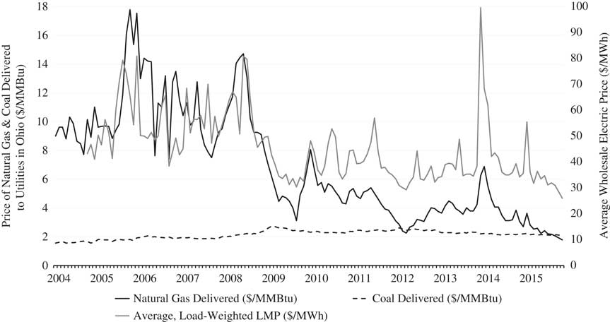
Another related competing argument would suggest that the residential price increases observed by households were owing to increases in wholesale costs associated with generation (e.g. fuel costs, pollution compliance). This alternative argument is misinformed. Because Ohio also restructured its wholesale markets, all generation in Ohio bids into the larger PJM regional market. Generation-related costs are incorporated into the wholesale price. To illustrate wholesale market developments, in Figure 4 we provide the average historical wholesale price of electricity observed by distribution utilities in Ohio, alongside the prices of the predominant fuel inputs of natural gas and coal. Both natural gas and coal price provide the final delivery price (inclusive of shipping costs) to electric generation units in Ohio. The wholesale price provides monthly load-weighted average locational marginal price (LMP) based on hourly load and pricing data from PJM and the Midcontinent Independent Systems Operator (MISO). It is noteworthy that we observe across the board significant price declines in the final wholesale price of electricity, inclusive of all generation-related costs, coincident with the shale boom during which prices for the marginal market clearing generation resource, natural gas, declined. Given this, arguments that residential price increases observed by households are due to increases in some unexplained components of wholesale costs are misguided.
Wholesale price of electricity, natural gas and coal in Ohio. Note: Values in inflation-corrected dollars per million metric British Thermal Units (BTUs) for gas and coal, and megawatt hours (MWh) for electricity. Wholesale prices reflect the average of each utility’s zonal load-weighted locational marginal price (LMP). Each utility’s load-weighted LMPs are calculated using hourly price and load data from PJM Interconnection, Midcontinent Independent Systems Operator and MarketViews. Natural gas and coal prices reflect the monthly final delivery price of each to electric generation in Ohio (inclusive of transportation costs). Source: EIA Electric Power Monthly (EPM), Table 4.10A. The spike in January 2014 reflects the Polar Vortex.
A core theoretical objective of deregulation is to bring retail and wholesale prices closer towards convergence, so that consumers’ fortunes are not tied to the fortunes of any one regional monopoly. It is striking that, with the implementation of retail restructuring in Ohio, we observe an inverse relationship between historic price declines in wholesale markets and historic price increases in retail price. One would expect that some of the savings from the wholesale market would be passed on to households – the “promise” of deregulation. The fact that we observe this for only one utility (Duke Energy), and the fact that this was the only utility in the state to functionally – rather than corporately – divest (or unbundle) its generation, is of critical interest. Duke Energy sold the near entirety of its generation to the wholesale generation firm Dynegy, except for a small co-ownership in a rural cooperative. The other three utilities retained arms-length ownership of their generation assets, predominantly legacy coal plants, with the exception of the Davis-Besse nuclear plant owned by a FirstEnergy subsidiary. As such, except for Duke Energy, the other three utilities took long positions in coal when the shale boom hit. With the implementation of SB 221, regulatory provisions allowing single-issue ratemaking afforded utilities an expedient path to offset their generation losses through nonbypassable riders and surcharges. Duke Energy, by selling its generation assets, did not observe comparable losses and therefore did not have the same instrumental incentive to obtain riders and surcharges.
Our identification of welfare losses for residential customers bares important questions about the political economy of retail restructuring. Of particular interest is welfare transfers to utilities. Blumsack et al. (Reference Blumsack, Lave and Apt2008), for instance, argue that the efficiency gains realized by utilities under restructuring are not passed on to residential consumers owing to increased transaction costs and a reallocation of risk. Price (Reference Price2005), in her discussion of the welfare consequences of liberalisation in the United Kingdom, notes a variety of market power concerns through which incumbent utilities can exploit switching costs at the expense of the vulnerable residential class. In general, it is not apparent that retail restructuring can successfully eliminate complicated vestigial relationships and political pressure between utilities and regulators. Instead, our findings match the liberalisation “lesson” that incomplete or incorrect implementation risks substantial costs (Joskow Reference Joskow2008).
Finally, our research runs counter to arguments that there is a benefit to a high SSO insofar as it encourages switching behaviour. To the extent that we treat the SSO as distinct from CRES rates, this argument is challenged by the substantial number of customers who have not switched. Moreover, it is important to bear in mind that distribution utilities are indifferent regarding switching rates because they observe no direct change in revenue if switching rates change. They have no direct incentive to keep the SSO low to retain market share. In the extreme case of a 0% switch rate, all generation revenue would be passed on to CBP auction tranche winners and not retained by the utility. In the opposite extreme case of a 100% switch rate, all generation revenue would flow through to CRES suppliers. Similarly, our findings contrast arguments in support of the claim that the costs of retail deregulation are front-loaded (mostly through stranded cost recovery) and the benefits are back-loaded. There is no immediate evidence to suggest that riders and tariffs will not continue to grow via subsequent regulatory action.
Retail restructuring has brought with it the ability for residential customers to exercise their Tieboutian option to “vote with their feet”. Customers can switch away from the SSO provided by the monopoly utility in their region and contract with a CRES provider. This behaviour can provide a variety of benefits outside the scope of this study. However, we similarly acknowledge that under Ohio’s retail restructuring regime, the majority of the riders, surcharges and T&D charges are unchanged by opting out to a CRES provider. Thus, any potential benefits of switching are heavily muted.
Conclusions and implications
The promise of retail electric deregulation was that moving to a market-based pricing system would set more favourable rates for households than prices determined exclusively by a regulatory commission. This article provides a quasi-experimental analysis of retail electric prices for all investor-owned utility service territories in the State of Ohio. It provides a controlled pre- and post-test of the effect of retail electric restructuring on residential SSO prices that are paid by millions of households. The results bring into relief the contrast between theory and practice. For most of Ohio’s residential retail load, prices have not declined since retail restructuring. For four of the seven metro areas in the state, retail restructuring resulted in higher month-to-month price trends than existed before restructuring. In addition, although the other three territories of Cincinnati, Columbus and Dayton have seen month-to-month price trends either not change or decline, relative to pre-restructuring, households in those territories paid a higher real (inflation-adjusted) price, on average, in the period following restructuring than they did in the period preceding. At a time when wholesale electricity prices were historically low, millions of households observed price increases despite price declines in the markets upon which their rates were supposedly based.
The ultimate question that this article should motivate is whether the observed failures are because of the manner in which retail deregulation was implemented or because of failures inherent to the underlying deregulatory theory. We would argue the former without jumping unnecessarily to the latter. Students and scholars of the public policy process have long understood many of the core pitfalls of policy implementation (Sabatier and Mazmanian Reference Sabatier and Mazmanian1980; Mazmanian and Sabatier Reference Mazmanian and Sabatier1981; Huber and Shipan Reference Huber and Shipan2002; Hill Reference Hill2003). In complex policy environments that require advanced knowledge, such as electricity markets, policymakers tend to ascribe a high degree of discretion to technical experts, such as public utilities commissions (Radaelli Reference Radaelli1995, Reference Radaelli2004; Esterling Reference Esterling2009). The Ohio legislature, in drafting the two pieces of legislation that initiated retail deregulation (SB 3 and later SB 221), diverged from the standard “textbook” model of retail restructuring that called for unbundling, or divestiture, of electric generation (power plants) from distribution (local service). They did this by requiring “corporate”, rather than functional, separation. In using this ambiguous language, they afforded a high degree of deference to the commission to implement this core prerequisite of deregulation.
Both policy scholars and political economic theorists recognise that statutory ambiguity, combined with a high degree of discretion exercised by implementers, creates conditions that cultivate rent-seeking (Krueger Reference Krueger1974; Wright Reference Wright1977; Tullock Reference Tullock2001; Mahoney and Thelen Reference Mahoney and Thelen2010; Carter et al. Reference Carter, Weible, Siddiki, Brett and Chonaiew2015). In this article, we identify two implementation steps taken by the commission that we believe drive the results of this study. One, in approving each public utility’s corporate separation plan, they permitted a broad statutory application that allowed utilities to create arms-length affiliate corporations to which they divested their plants (almost entirely legacy coal). Two, they allowed utilities to pursue a hybridised tariff system, known as an ESP, that permitted utilities to add nonbypassable riders (almost three dozen) to household electric bills. Ohio’s retail restructuring legislation (SB 221) required that utilities eventually transition to only using competitively determined MROs for setting SSO rates, and also created an ESP versus MRO test to ensure that ESPs were more favourable in the aggregate as compared with MROs. However, by adopting broad language for this test and not establishing a timeline to adopt MROs, the legislature again deferred to the PUCO.
PUCO, in enforcing ESPs, adopted “single-issue” ratemaking approval for ESPs rather than comprehensive regulatory review, meaning proposed costs are subject to less rigorous review than before retail restructuring. As a consequence, utilities have wide discretion to pursue riders as a nonbypassable revenue source imposed on all customers. In the historical context of the shale boom, this created a rent-seeking incentive in order to offset the losses of a predominantly coal fleet relative to natural gas competition in wholesale markets. A more textbook implementation of deregulation would have privatised those losses and shielded customers as a result.
The above implementation failures are illuminated by the data for the Cincinnati metro area (Duke Energy). Duke Energy is the only utility in the state that pursued functional divestiture. It is the only metro area in the state that observed a reversal of the pre-retail restructuring price trend and substantial welfare gains. Unlike the other utilities in the state, Duke Energy did not have an ageing coal fleet indirectly on their balance sheets and, therefore, no instrumental incentive to socialise private losses.
Although many prior studies have approached this issue with more breadth, such as national or multistate studies, we approached this issue with greater depth by digging deeper into the dynamics of a major deregulated state. We believe that the issues identified in this article highlight important aspects of restructuring, and policy implementation more broadly, that should inform many other states and nations. We thus maintain that, in most states, simply declaring a state “regulated” or “deregulated” is too simplistic, devoid of fundamental institutional dynamics. Rather, we suggest that restructuring exists on a continuum of degrees of commission intervention. Ohio does not have completely deregulated retail markets according to theoretical definitions, but it does reflect vestiges of commission control and utility intervention that are present in many peer states.
States such as Ohio have two choices in addressing flaws associated with restructuring; movement towards reregulation, or greater market-basis pricing with less commission intervention. Although the former would represent a near reversal of current policy towards an established outcome, the latter represents policy adjustment towards a less clear path forward. Thus, although we feel that we have informed the overall question of whether markets make good commissioners, we reflect on the perhaps equally important question of whether commissioners make good markets.
Acknowledgements
The authors thank the Battelle Center for Science and Technology Policy at the John Glenn College of Public Affairs for its generous support. The authors are grateful to Asma Diallo for valuable research assistance. The following individuals and organisations are also recognised for important comments and support in this work: William Michael, Edward Hill, Dorothy Bremer, Pat Frase and the PUCO. Any errors or omissions are solely those of the authors.
Appendix
Table A.1, Table A.2, Table A.3, Table A.4, Table A.5, Table A.6.
Key market events in the history of Ohio’s four major investor-owned utilities
Number and proportion of residential customers facing standard service offer rates by each utility and major city
Dickey-Fuller tests
Variance ratio tests on electricity prices
Reset results for nonlinearity

Portmanteau and Bartlett’s white noise tests of residuals